Using Uncrewed Aerial Vehicles for Identifying the Extent of Invasive Phragmites australis in Treatment Areas Enrolled in an Adaptive Management Program

Abstract

Higher spatial and temporal resolutions of remote sensing data are likely to be useful for ecological monitoring efforts. There are many different treatment approaches for the introduced European genotype of Phragmites australis, and adaptive management principles are being integrated in at least some long-term monitoring efforts. In this paper, we investigated how natural color and a smaller set of near-infrared (NIR) images collected with low-cost uncrewed aerial vehicles (UAVs) could help quantify the aboveground effects of management efforts at 20 sites enrolled in the Phragmites Adaptive Management Framework (PAMF) spanning the coastal Laurentian Great Lakes region. We used object-based image analysis and field ground truth data to classify the Phragmites and other cover types present at each of the sites and calculate the percent cover of Phragmites, including whether it was alive or dead, in the UAV images. The mean overall accuracy for our analysis with natural color data was 91.7% using four standardized classes (Live Phragmites, Dead Phragmites, Other Vegetation, Other Non-vegetation). The Live Phragmites class had a mean user’s accuracy of 90.3% and a mean producer’s accuracy of 90.1%, and the Dead Phragmites class had a mean user’s accuracy of 76.5% and a mean producer’s accuracy of 85.2% (not all classes existed at all sites). These results show that UAV-based imaging and object-based classification can be a useful tool to measure the extent of dead and live Phragmites at a series of sites undergoing management. Overall, these results indicate that UAV sensing appears to be a useful tool for identifying the extent of Phragmites at management sites.

1. Introduction

Over recent decades, invasive exotic plant species have become a growing concern in the ecological restoration community due to their detrimental impacts on biodiversity and ecosystem function as well as their economic costs ([1,2]). Wetlands in particular provide a range of valuable ecosystem services, such as flood protection and water filtration. However, they can be particularly susceptible to invasion by introduced species, in part because they are landscape sinks, with augmented nutrient loading from upstream and/or adjacent landscape areas, and impacted by hydrological disturbances and variation ([3]). The introduced European genotype of Phragmites australis (Cav.) Trin. ex Steud. (common reed) has been a nuisance in the Great Lakes region since the mid-20th century ([4]), impacting habitat availability for native species, among other ecosystem services. Adequate monitoring and evaluation plans are needed to ensure the success of programs to restore these ecosystem functions, but there remains a need for well-defined goals and sufficient resources allocated to these activities ([5,6]). Long-term monitoring that spans a time period before, during, and after treatment is frequently included in recommendations for restoration best practices and is a fundamental component of adaptive management, yet may be overlooked ([1,5,7]). Hazelton et al. [8] have noted that additional tools to measure the outcomes of Phragmites treatment programs are needed. The development of efficient, low-cost methods to help monitor restoration outcomes could contribute to greater effectiveness of these types of restoration efforts by providing easier access to quantitative information on success metrics such as biodiversity, species distribution, and abundance statistics.

Traditional remote sensing methods via platforms such as satellite or crewed aircraft can be useful for ecological monitoring efforts, particularly for large or broadly distributed sites ([9,10]). Those methods offer a means of efficiently assessing broad swaths of land without the time-intensity of detailed field surveys. However, those methods can also be prohibitively expensive or produce data at spatial resolutions too coarse and/or temporal resolutions too infrequent to derive useful information. Alternative methods to obtain higher-resolution data in a cost- and time-efficient manner would be more useful for monitoring treatment effectiveness.

Uncrewed aerial vehicles (UAVs, also referred to as small uncrewed or unmanned aircraft systems/sUAS, remotely piloted aircraft systems/RPAS, or commonly “drones”) have been increasing in capability in recent years and are becoming more practical platforms for providing the type of relatively low-cost, high-resolution remote sensing data that can be very useful for monitoring wetland sites ([11,12,13,14]). Examples of useful ecological applications of drones include studying time-dependent phenomena such as tidal patterns and water stress, identifying submerged aquatic vegetation taxa, and mapping canopy gaps and precision agriculture ([12,15,16]). Whereas more traditional, field-based surveys can often be labor-intensive and difficult to complete in remote areas, UAVs can offer a safer, more time- and cost-efficient monitoring method that could potentially help capture the impacts of invasive plants, especially when augmented with some degree of ground-truth data. In the case of invasive species monitoring, this method can provide on-demand imagery with the spatial and temporal resolution needed to detect the presence and/or removal of target species.

Recent research and other projects have demonstrated that UAV-enabled sensing can help with mapping non-native wetland plant extent and inform monitoring of treatment sites. Mapping Phragmites and other emergent wetland plants with natural color and near-infrared imagery has been demonstrated in several projects and publications [17,18,19,20]. Samiappan et al. [19] used UAV imagery to map invasive Phragmites near the Gulf Coast in Louisiana. They used a UAV with a MicaSense RedEdge sensor to acquire high-resolution multispectral imagery that included blue, green, red, red edge, and near infrared spectral bands. These bands, in addition to digital surface models and vegetation indices, were used to perform a supervised classification for the site through the Support Vector Machines classification method. Similarly, Jensen et al. [17] developed a multispectral UAV remote sensing platform to monitor wetlands and predict future extents of Phragmites australis in Utah’s Bear River Migratory Bird Refuge. Zhou, Yang, and Chen [20] used UAV data in tandem with SPOT6 multispectral satellite imagery to estimate the biomass of invasive Spartina alterniflora in the Sansha Bay near Fujian, China. Lishawa et al. [18] compared UAV data with in-situ information to document the mechanical harvesting of invasive Typha spp. (cattail) on the St. Mary’s River, Michigan. For submerged aquatic vegetation, Brooks [15,21] used UAV imagery to detect the invasive Eurasian watermilfoil (Myriophyllum spicatum) in Michigan.

These examples demonstrate that UAV-enabled sensing of invasive wetland and submerged aquatic plants is feasible. However, specifically using high-resolution UAV imagery for quantifying treatment outcomes does not appear to be as common. This paper focuses on how UAV sensing could be applied for evaluating Phragmites extent at 20 sites enrolled in an adaptive management program that sometimes led to Phragmites removal depending on landowner interest. Here, adaptive management refers to a land and resource management strategy that uses repeated monitoring to learn from management outcomes and incorporate that information into future planning ([22]). Monitoring and learning are key components of this strategy, which presents an opportunity for the use of UAVs for timely collection of monitoring data. If this type of sensing could help quantify Phragmites extent, then UAVs could be a practical part of monitoring programs. Understanding if UAVs could help identify Phragmites presence and extent, particularly after treatment programs to remove this species, was an interest of the sponsoring agency for this project (the U.S. Geological Survey) and the Phragmites Adaptive Management Framework (PAMF) program.

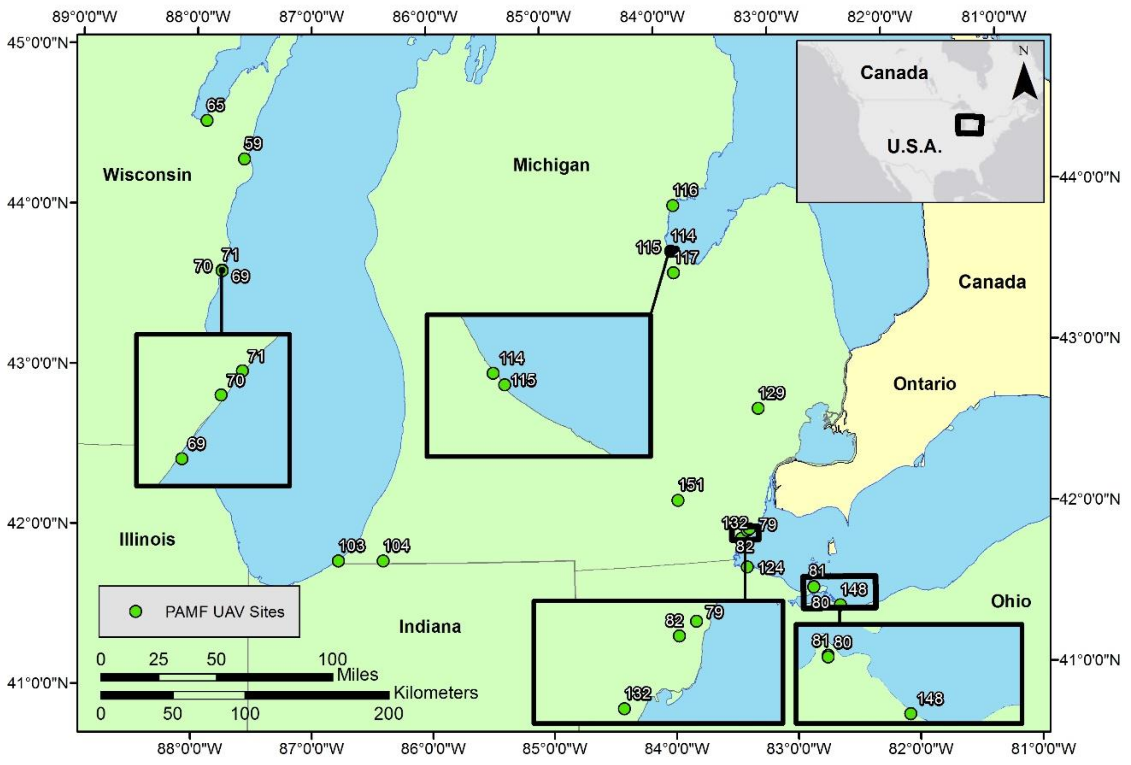
The goal of this research was to assess the value of UAV-based imaging in tandem with an object-based image classification approach to help with monitoring the effectiveness of Phragmites australis control treatments in the Great Lakes basin. We worked in 20 coastal Great Lakes sites (Figure 1) that were enrolled in the PAMF program, which collects Phragmites treatment and outcome information from land managers, inputs that data into a model, and then provides data-driven treatment recommendations (https://www.greatlakesphragmites.net/pamf/ (accessed on 22 March 2021)).

Our objective was to demonstrate the ability to map different types of vegetation present, focusing on live and dead Phragmites, in treatment monitoring areas by combining drone imagery with field surveys. To achieve this, we deployed a UAV equipped with a natural color red/green/blue (RGB) camera while also documenting the major vegetation types observed in the field. We also deployed a low-cost near infrared (NIR) camera at two sites on a demonstration basis. We then used these data to generate classifications with a nearest neighbor method. The resulting classifications were validated and assessed through comparison with visual interpretation of the vegetation classes in the imagery. The accuracy of our results was assessed using error matrices using the methods described in Congalton and Green [23].

2. Materials and Methods

2.1. Site Selection

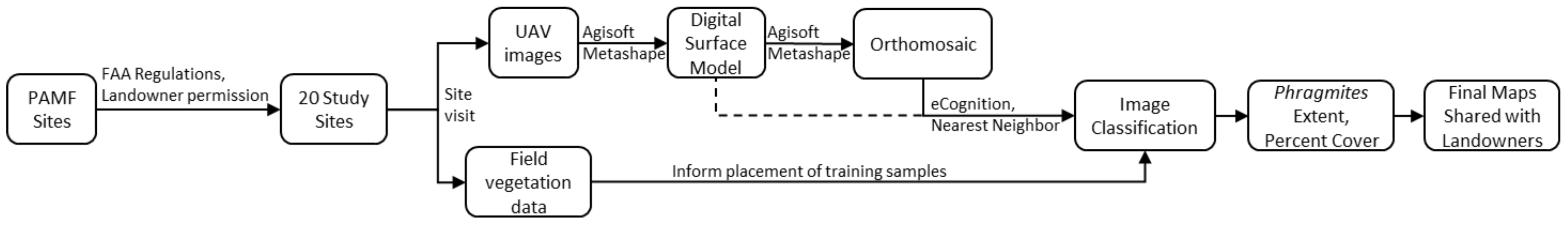
A flow chart of the workflow of this study is shown in Figure 2. Study sites were chosen in collaboration with PAMF project leaders. Through this program, land managers collect and share information about the treatment methods and outcomes of their enrolled property using a standardized set of monitoring protocols. This project’s goal was to collaborate with PAMF managers to test and demonstrate a method of incorporating rapid, high-resolution UAV-collected imagery into monitoring efforts. Each of the 34 candidate sites, enrolled in the PAMF program and selected by the program managers for potential study, was reviewed for site accessibility constraints, possible hazards to UAV operations, and compliance with U.S. commercial small UAV rules from the Federal Aviation Administration (known as “Part 107”). In total, 20 of the original 34 candidate sites were appropriate for UAV flight operations based on airspace restrictions and site access. The sites included in this study are located in Michigan, Wisconsin, and Ohio, USA (as shown in Figure 1), and the management unit boundaries were provided by PAMF participants when they enrolled in the program. The sites range in area from 0.01 ha (Site 129) to 5.38 ha (Site 116), with an average area of 0.98 ha. The sites also range in type, including land managed by state and federal agencies, as well as private owners. All sites were surveyed with landowner permission.

2.2. UAV-Enabled Sensing Design

Two UAV platforms were used for this study: the DJI Phantom 3 Advanced and the DJI Mavic Pro. The specifications of both are summarized in

Table 1. Specifications of the two UAV platforms used for the study: the DJI Phantom 3 Advanced and the DJI Mavic Pro.

	DJI Phantom 3 Advanced	DJI Mavic Pro
Cost	$1200 U.S. at time of purchase	Relatively low ($1300 USD at time of purchase)
Weight	1.28 kg	0.74 kg
Camera resolution	12.4 MP, 2.7 k video	12.4 MP, 4 k video
Camera mount	3-axis gimbal	3-axis gimbal
Field of view	94°	78.8°
Ground sampling distance (GSD)	Up to 6.6 cm at 122 m altitude	Up to 5 cm at 122 m altitude
Maximum flight time	23 min	27 min
Maximum flight speed	56 kph	65 kph

below. Both platforms are relatively low-cost (US $1000 to $1500 at the time of purchase) and lightweight (1.28 kg for the Phantom 3 and 0.74 kg for the Mavic Pro), which makes them ideal for collecting data in locations that may be difficult to reach in the field.

In addition to the standard optical RGB camera, we also mounted a MAPIR Survey 3 camera with NIR, red, and green bands to the Phantom 3 UAV for initial testing purposes, using a custom-created mounting platform that fit on the bottom of the Phantom 3 between the two landing legs. We collected data at two separate sites with the sensor in addition to standard RGB optical imagery to test whether this low-cost (U.S. $400) sensor with a NIR band could improve mapping of the project sites. The sensor was only available for these two sites. 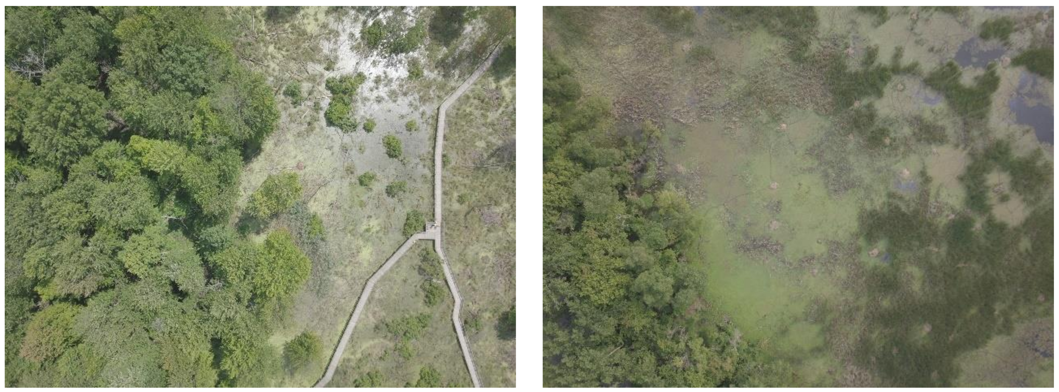This sensor collected 12MP images with an 87° field of view, which were used for this study (example shown in Figure 3). This approach provides a ground sample distance (GSD) of approximately 5 cm at 122 m above ground level (AGL). In addition to collecting imagery, the Survey 3 camera also collected GPS position and altitude information, which aided in mosaicking the imagery. A comparison between the optical RGB and near-infrared composite can be seen in Figure 4.

2.3. Flight Mission Planning and Data Acquisition

Both field and UAV data were collected for each of the sites, once between July and September 2018 (see

Table 2. Study site characteristics, including type of site and approximate flight times.

Site Number	Site Type	Flight Times of Day (Approx.)
59	emergent	9/15/18 14:45
65	emergent	9/4/18 17:00
69	beach	9/5/18 09:00
70	beach	9/5/18 11:00
71	beach	9/5/18 11:00
79	emergent	8/15/18 11:30
80	emergent	8/3/18 12:30
81	wet meadow	8/3/18 12:45
82	emergent	8/15/18 10:30
103	emergent	9/6/18 15:00
104	emergent	9/6/18 16:15
114	coastal forest	8/10/18 10:45
115	emergent	8/10/18 11:30
116	emergent	8/10/18 09:15
117	emergent	8/10/18 16:30
124	emergent	8/3/18 14:45
129	unavailable	unavailable
132	emergent	8/3/18 15:45
148	wetland forest	8/3/18 11:00
151	emergent/wetland shrub/wetland forest	7/31/18 09:00

). These field data collections were informed by a set of overview maps that included site information such as site boundaries, latitude, longitude, site scale, and a representative basemap. These overview maps were brought into the field and used to inform both the UAV flight path and vegetation characterization.

For this study, the UAV was programmed to fly in a grid pattern over the treatment region 100 m above ground level, with 70% forward overlap and 60% side overlap, using the Pix4DCapture mobile phone application. Each programmed flight captured still images (between 33 and 649 images per site, depending on site size) at fixed intervals, camera angles (at nadir), and speed to ensure complete area coverage and adequate image overlap for 3D reconstruction. Flights were performed between morning and mid-late afternoon. Positional accuracy was determined by the onboard GPS of the Phantom 3 and Mavic Pro, with about 3 to 5 m being typical. Once complete, the team manually captured oblique UAV imagery of the site. All imagery was quality-checked on site, both as it was collected using FPV capabilities and also after data collection.

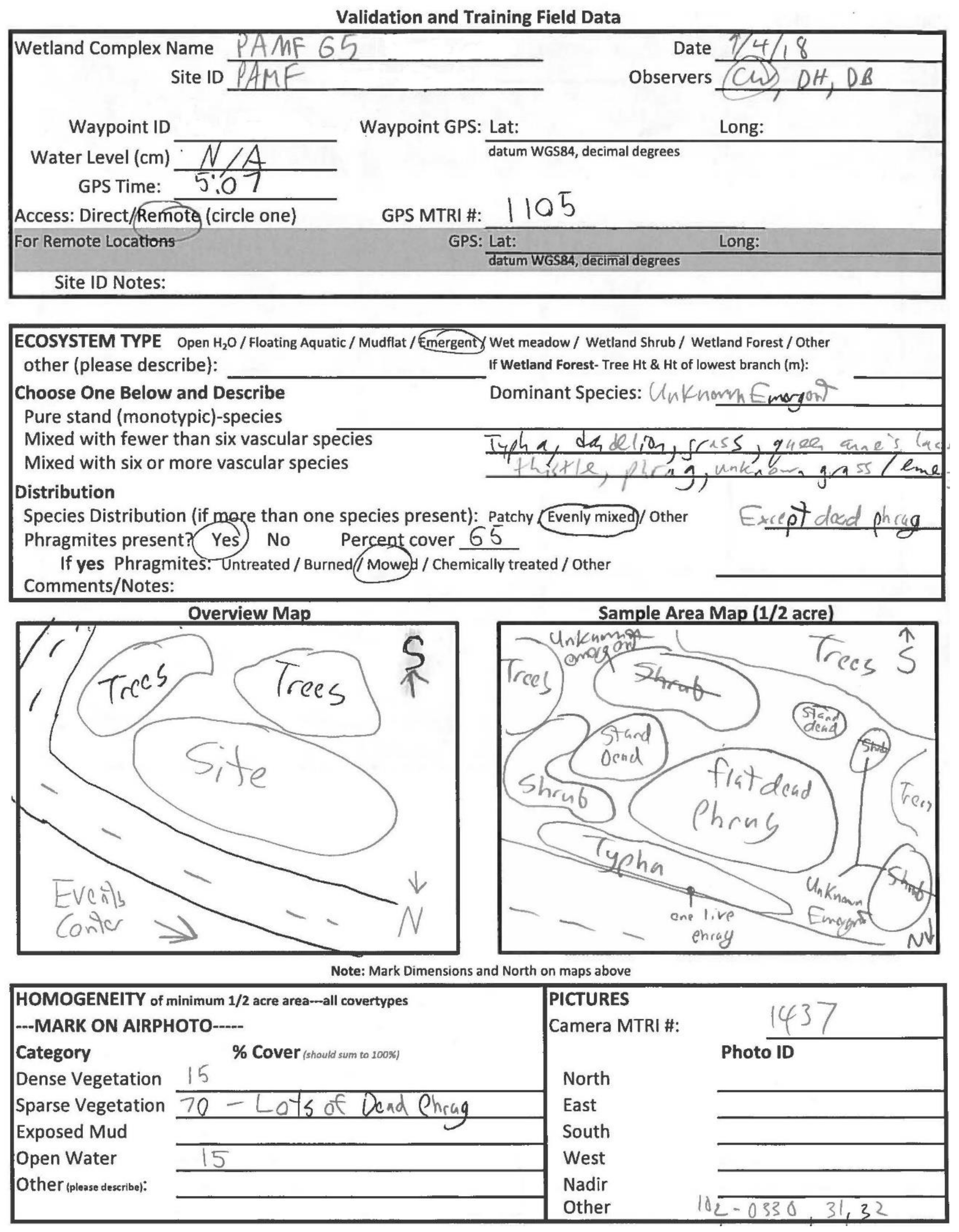
In addition to the UAV imagery, field technicians also collected standardized vegetation data at each site. These data included dominant cover types, a list of other plant species present, and a sketch of the vegetation distribution across the site, including the locations of both dead and living Phragmites within the study region; Figure 5 shows an example of a field sheet with recorded data. The locations of these vegetation types were also marked on the overview figures to assist with UAV imagery classifications. Field observers also collected geotagged ground digital photos, which served as a second source of imagery to inform image classifications.

2.4. Data Processing and Image Classification

The team created orthomosaic and digital surface model (DSM) products of each site using Agisoft Metashape (Agisoft, St. Petersburg, Russia, 2019).

Table 3. Agisoft Metashape settings used to process the UAV imagery into orthophoto and DSM products.

1.	Align Photos Settings:
	a.	Reference preselection
	b.	High accuracy
	c.	Key point limit—40,000
	d.	Tie point limit—4000
2.	Build Dense Cloud Settings:
	a.	Quality—High
	b.	Depth Filtering—Aggressive
3.	Build Mesh Settings:
	a.	Source data—Dense Cloud
	b.	Surface type—Height Field
	c.	Interpolation—Disabled
4.	Build DEM (Default settings):
	a.	Type—Geographic
	b.	Interpolation—Enabled
5.	Build Orthomosaic (Default settings):
	a.	Type—Geographic
	b.	Surface—DEM
	c.	Blending Mode—Mosaic
	d.	Enable Hole Filling is selected

summarizes the main Metashape parameters used to create the output products from the UAV imagery. The team first created a sparse image point cloud within the program using close-range photogrammetry. After confirming that the point cloud contained accurate GPS positioning information and that the images were correctly merged, the dense point cloud and mesh were generated. The DSM was then created using the completed mesh. The orthomosaic was generated next matching the extent of the DSM.

UAV imagery was used to generate land cover maps using object-based image analysis in Trimble’s eCognition Developer version 9 software (Trimble Inc., Sunnyvale, CA, USA). These cover maps relied primarily on the orthomosaic. For some sites, the DSM was also included because we anticipated that plant height could help differentiate between cover classes; for sites without visibly significant height variation, we did not include the DSM as initial investigations showed it did not appear to contribute to higher accuracy results, based on the expert judgment of our image interpreters. After loading the layers into eCognition, the next step was to execute multiresolution segmentation on each mosaic. This command breaks down each mosaic into polygons based on spectral similarities amongst neighboring pixels in the frame, according to a preset segmentation scale parameter (for this study, a number between 10 and 65 based on the expert judgment of our image interpreters). Once this step was completed, the team next used field notes and field photos to create training data for each land cover type. Once sufficient training data had been provided, we executed the classification step. This study used eCognition’s nearest neighbor classification method, which compares user-selected polygon information such as mean RGB pixel values, brightness, contrast, standard deviation, and elevation data (using the DSM) to make class assignment decisions. The classification assigns a cover type to all regions of the image based upon the characteristics of the training data polygons and the input parameters. Classification results were exported as a raster file, projected to the locally appropriate Universal Transverse Mercator (UTM) zone with the World Geodetic System of 1984 (WGS84) datum, and then used to calculate the percent cover of Phragmites compared to other vegetation types within the PAMF-enrolled management unit.

Each of the sites was classified separately using a customized set of rules with the nearest neighbor classification tool in eCognition. All of these rulesets included mean pixel value for the RGB bands (along with the DSM, for those sites that used this band). The resulting classification served as a useful starting point for iterative improvements to the classifications of each of the sites.

Use of additional spectral or geometric rules depended upon the unique characteristics of that site. For example, in site 59, use of the ‘x distance to scene right border’ rule allowed the classification to take into account the presence of a road along the right-hand border of the image and distinguish “road” and “car” classifications from other bright pixels. Position-distance inputs like this one were used to generate 6 out of the 20 final classifications. Other commonly-used types of rules included standard deviation (used for 8 sites), ratio (8 sites), and hue (RGB, 7 sites), using the expert judgment of our image analysists. Additionally, the Visible Atmospherically Resistant Index (VARI), which is calculated using the red, green, and blue bands, was used for distinguishing between vegetation types at 6 of the sites. Each classification was developed using a highly iterative process and then quality-checked by another member of the team. When possible, the image was reviewed by a teammate who had visited that site in person.

Table 4. Layers and classification parameters used for each site. The first column lists the site name. The second column identifies the imagery bands used to generate the image classification in eCognition, including red green blue (RGB) and/or the digital surface model (DSM). The third column identifies the scale parameter used in the initial image segmentation. The remaining columns identify the specific parameters used in the image classifier, organized based upon the same categorical hierarchies as they appear in eCognition.

			Object Features															Class-Related Features
			Customized					Layer Values							Geometry		Position	Relations to Neighbor obj.
			VARI	NDVI	Other 1	Other 2	Other 3	Mean	Std. Dev.	Pixel-Based		To Neighbors	Hue, Saturation, Intensity		Extent	Shape	Dist.	Rel. Border to
Site Name	Bands Used	Segmentation Scale Parameter								Ratio	Edge Contrast of Neighbor Pixels	Mean Diff. to Neighbors (abs. Value)	Hue	Saturation	Area (Pixel)	Round-Ness
Site59	RGB	50	X					X	X	X		X	X		X		X	X
Site65	RGB	10						X	X				X
Site69	RGB, DSM	10						X	X	X
Sites70-71	RGB, DSM	10						X		X			X
Site79	RGB	65				X		X
Site80	RGB	10	X					X									X
Site81	RGB, DSM	25	X					X		X	X		X					X
Site82	RGB, DSM	20	X					X						X			X
Site103	RGB	30						X	X								X
Site104	RGB, DSM	30						X					X
Site114	RGB, DSM	20						X									X
Site115	RGB, DSM	10	X				X	X	X	X				X			X
Site116	RGB, DSM	30			X			X								X	X
Site117	RGB, DSM	10						X	X								X
Site124	RGB, DSM	10						X		X			X
Site129	RGB, DSM, NIR	50		X				X	X
Site132	RGB	30	X					X	X									X
Site148	RGB, DSM	50						X		X		X		X			X	X
Site151 RGB	RGB, DSM	10						X		X			X
Site151 NIR	RGB1, DSM, R2, G2, NIR	25		X				X									X
Count totals:			6	2	1	1	1	20	8	8	1	2	7	3	1	1	10	4
* R2 and G2 are the red and green bands from the NIR Camera
In Site151 NIR the Red, Blue, and Green Bands used for classification were the Red and Green Bands from the NIR camera and Blue band from orthoimagery Other 1: (R−DSM)/(R+DSM−G) Other 2: ((X distance to scene left border)^2 + (Y distance to scene top border*1.5)^2)^0.5 Other 3: (X distance to scene left border)^2 + (Y distance to scene bottom border)^2
Most commonly used:
Rule type									# of sites
Mean									20
Position									10
Std. Dev.									8
Ratio									8
Hue									7
VARI									6
Rel. border to									4
Saturation									3
Mean diff. to neighbors									2
NDVI									2

describes the bands, segmentation parameters, and rules used for each final classification. This iterative process with rules that could differ for each site enabled us to optimize the classification result to have highest accuracy based on field data and the experience of the image analysts. The majority of columns in Table 4 are categorized as “Object Features,” meaning they utilize values of the image objects—in our case, the individual image segments. Customized parameters involved the manual input of formulas using band values—these included VARI (visible atmospherically resistant index; an alternative to NDVI using only RGB wavelengths) and NDVI (normalized difference vegetation index). Customized values using distance took advantage of the specific spatial characteristics of a site, e.g., if an image included a road along the southern edge. Parameters falling under the “Layer Values” category were standard options available in eCognition that rely on the band values for each segment. These include mean, standard deviation, pixel-based ratio, and edge contrast of neighbor pixels, mean absolute value distance to neighbors, hue, and saturation. Geometry parameters use the geometric properties of the image segments, including extend (area) and shape (roundness). Class-related features take into account contextual information from a previously generated classification.

In addition to the stated classification parameters, the team was also able to repeat the classification process to include parameters such as mean NIR values and NDVI (Normalized Difference Vegetation Index) at the two sites where NIR imagery was collected. These parameters can be useful in cases where different species of vegetation have different spectral reflectance characteristics at near-infrared wavelengths. For example, Valderrama-Landeros et al. [24] leveraged the differing spectral profiles of two tree species Laguncularia racemose and Rhizophora mangle to map Mexican mangroves with an NDVI-based classifier. NDVI has also been useful for distinguishing phenological patterns in Northeast China ([25]) and Phragmites australis ([19]). 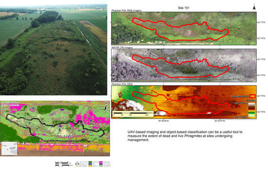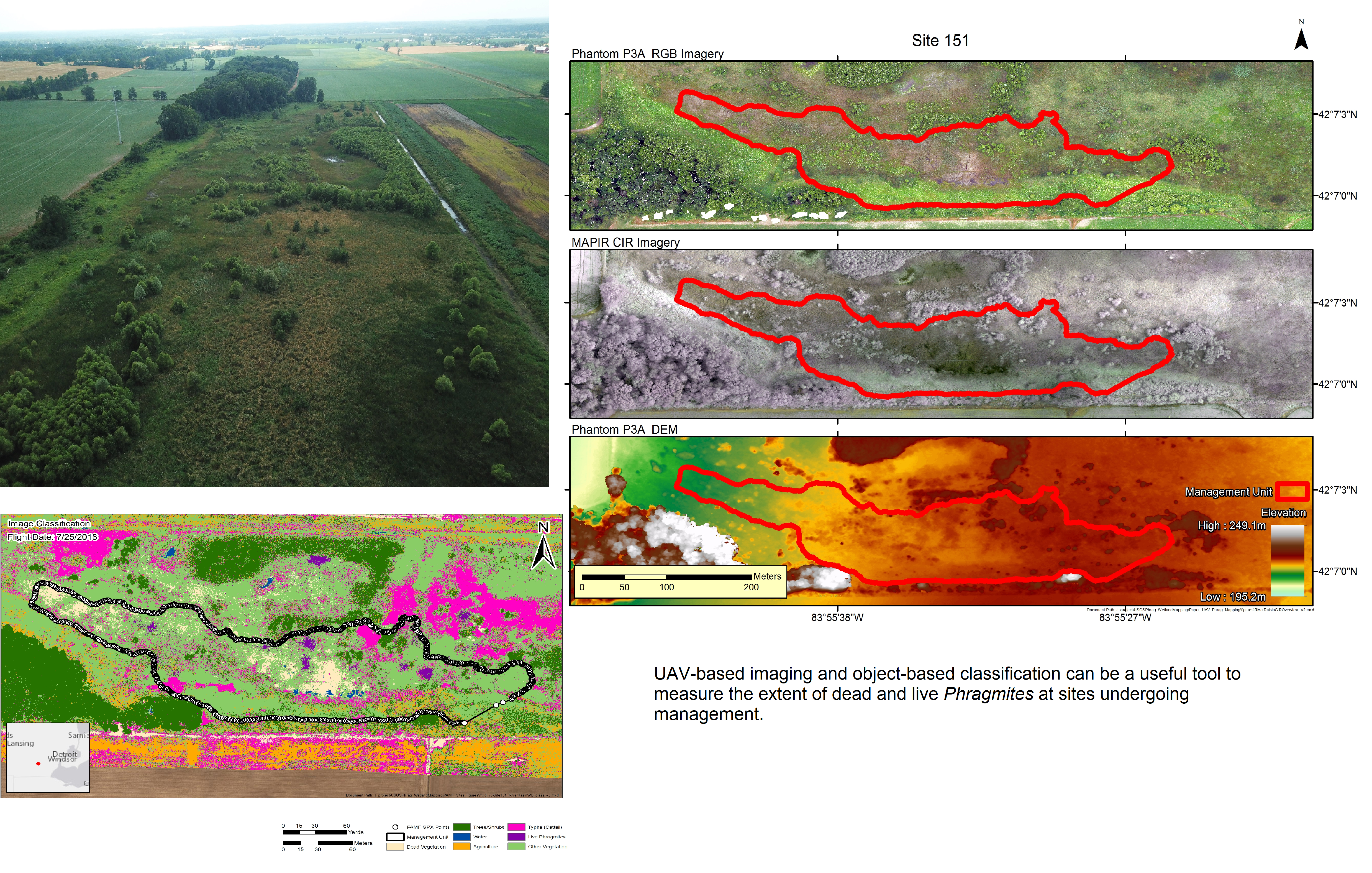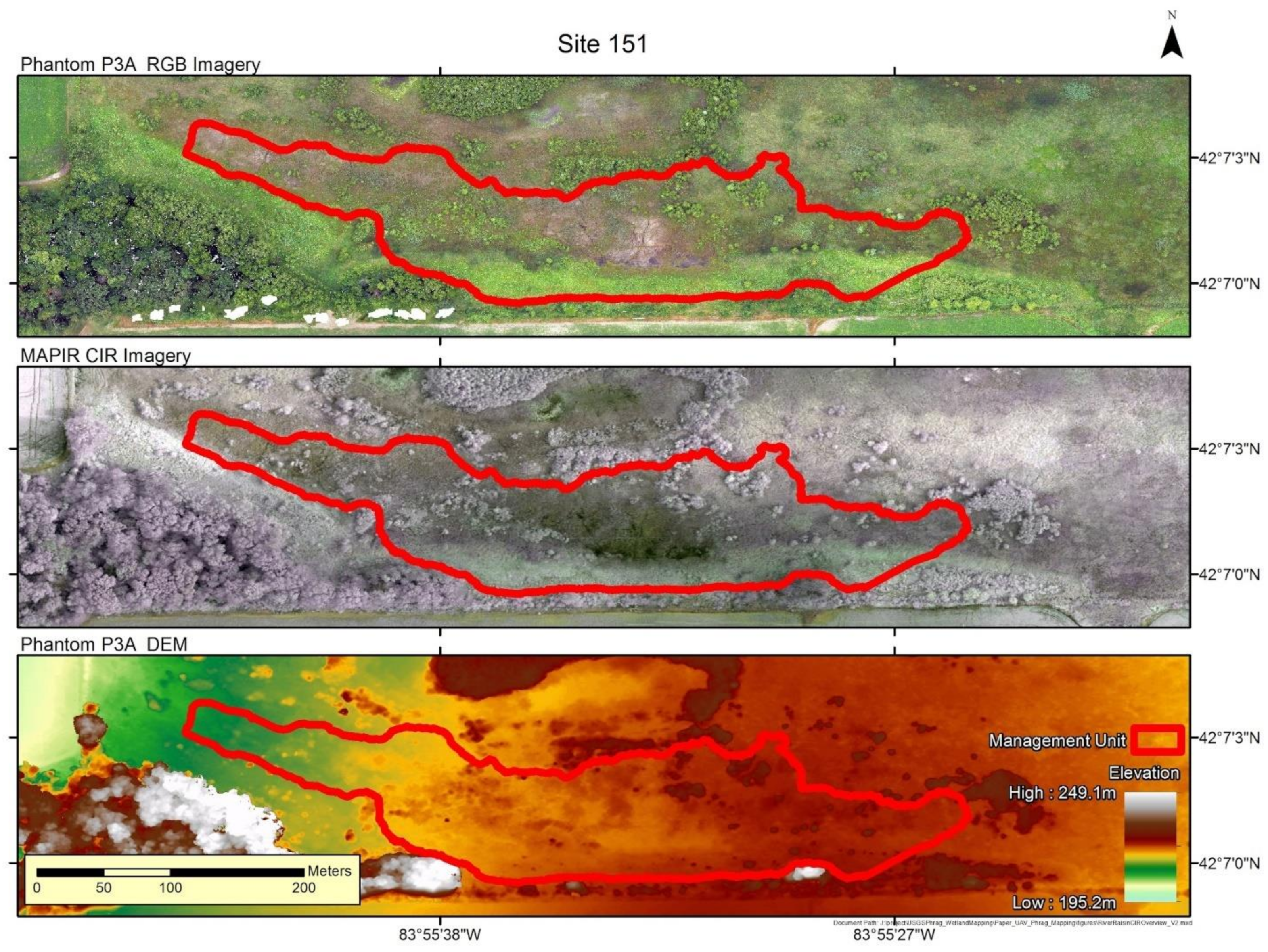Figure 6 shows examples of RGB and NIR imagery, along with DEM data for site 151. Results between the two classification techniques were compared to determine if the addition of NIR imagery significantly aids in the classification of Phragmites using UAV-derived imagery.

2.5. Classification Validation

Image classification accuracy can be assessed in a multitude of ways including visual appraisal, comparison to reference ground data sets, and accuracy metrics derived from confusion matrices, with one of the most popular methods being percentages reporting the overall and individual class accuracies ([23,26]). Here, accuracy assessment of the data followed the standard methods of Congalton and Green [23]. The assessment was done on each site using a visual comparison between what the classifier identified each point as, and what the team identified the point as through visual interpretation, similar to the validation methods used by Pande-Chhetri et al. [27]. This assessment utilized orthoimagery and ground photos to determine classification accuracy.

The number of sampling points at each site was determined using the multinomial distribution in the equation shown below as used by Congalton and Green [23]. In the equation, n is equivalent to the number of recommended samples.

$$n=B{\Pi }_i\left(1-{\Pi }_i\right)/b_i^2$$

(1)

For our assessment, we had a desired confidence level of 85% and a desired precision of 15% (represented as b in above equation). The Chi-squared (χ2) inverse of right tailed probability represented as B, is calculated with (α/k) = probability, assuming 1 degree of freedom. In this case, α is equivalent to desired precision, k is equivalent to the number of classes at each site, and ${\Pi }_i$ is equivalent to the percent cover of each class ([28]).

After determining the values of n for all classes within a study site, the largest of those values was then chosen as the required sample number for that site. From there, the sample number was next distributed to all classes by multiplying the recommended number of samples, by the percent cover within each class. Sample counts were then rounded to the nearest whole number. Based on the sample counts, the specified number of sample points was then generated within each class. This choice for random point selection follows the stratified random sampling method described in Congalton and Green [23].

In order to ensure consistency in the error assessment among all sites, the classes for each site were grouped into four distinct categories. These include Live Phragmites, Dead Phragmites, Other Vegetation, and Other Non-Vegetation. These four classes were chosen based on the purpose of this study to characterize the presence of Phragmites within our study areas. Other non-Phragmites cover types, such as roads, open water, or shrubs were not relevant to this research goal and were therefore aggregated into “Other Vegetation” and “Other Non-Vegetation” classes. The error assessment was then derived based on these four classes.

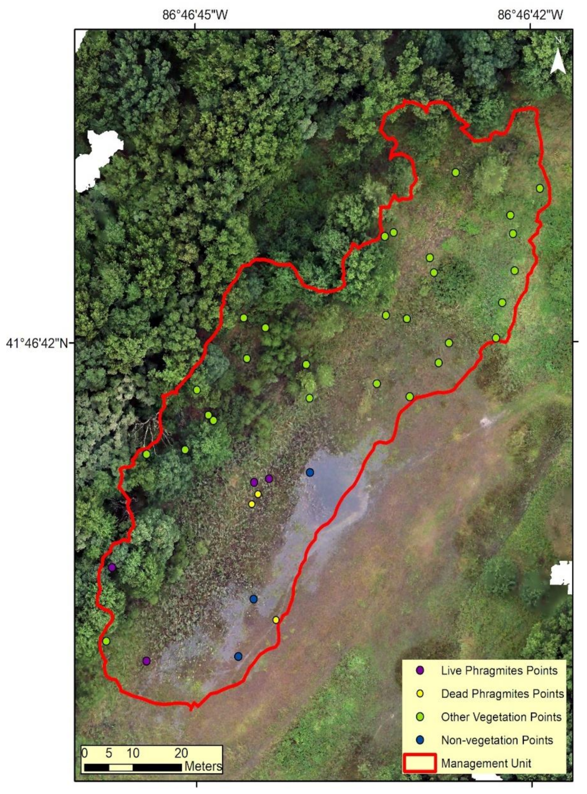
Once points had been selected and all classifications were standardized, the error assessment of each site was conducted, and an error matrix was created. Each matrix contains reference data along the horizontal axis and classified data along the vertical axis. Once complete, an overall accuracy was computed by summing the diagonal elements of the matrix and then dividing that sum by the totals for each row. In addition to overall accuracy, the producer’s and user’s accuracy were calculated for all four classes. This determines accuracy on a class by class basis. Examples of the placement of validation points and the error matrix for one site (103, Figure 7) are shown below in

Table 5. Example confusion matrix with validation results for Site 103. In this example, the classification at Site 103 had an overall accuracy of 89.5%. The live Phragmites user’s accuracy was 50.0%, the live Phragmites producer’s accuracy was 100%, the dead Phragmites user’s accuracy was 66.7%, and the dead Phragmites producer’s accuracy of 66.7%.

Site 103	Reference Data						User’s Accuracy
Classification Data		Live Phragmites	Dead Phragmites	Other Vegetation	Other Non Vegetation	Row Total
	Live Phragmites	2	1	1	0	4	50.0%
	Dead Phragmites	0	2	0	1	3	66.7%
	Other Vegetation	0	0	27	1	28	96.4%
	Other Non Vegetation	0	0	0	3	3	100%
	Column Total	2	3	28	5	38
Producer’s Accuracy		100%	66.7%	96.4%	60.0%
Overall Accuracy = 89.5%

.

3. Results

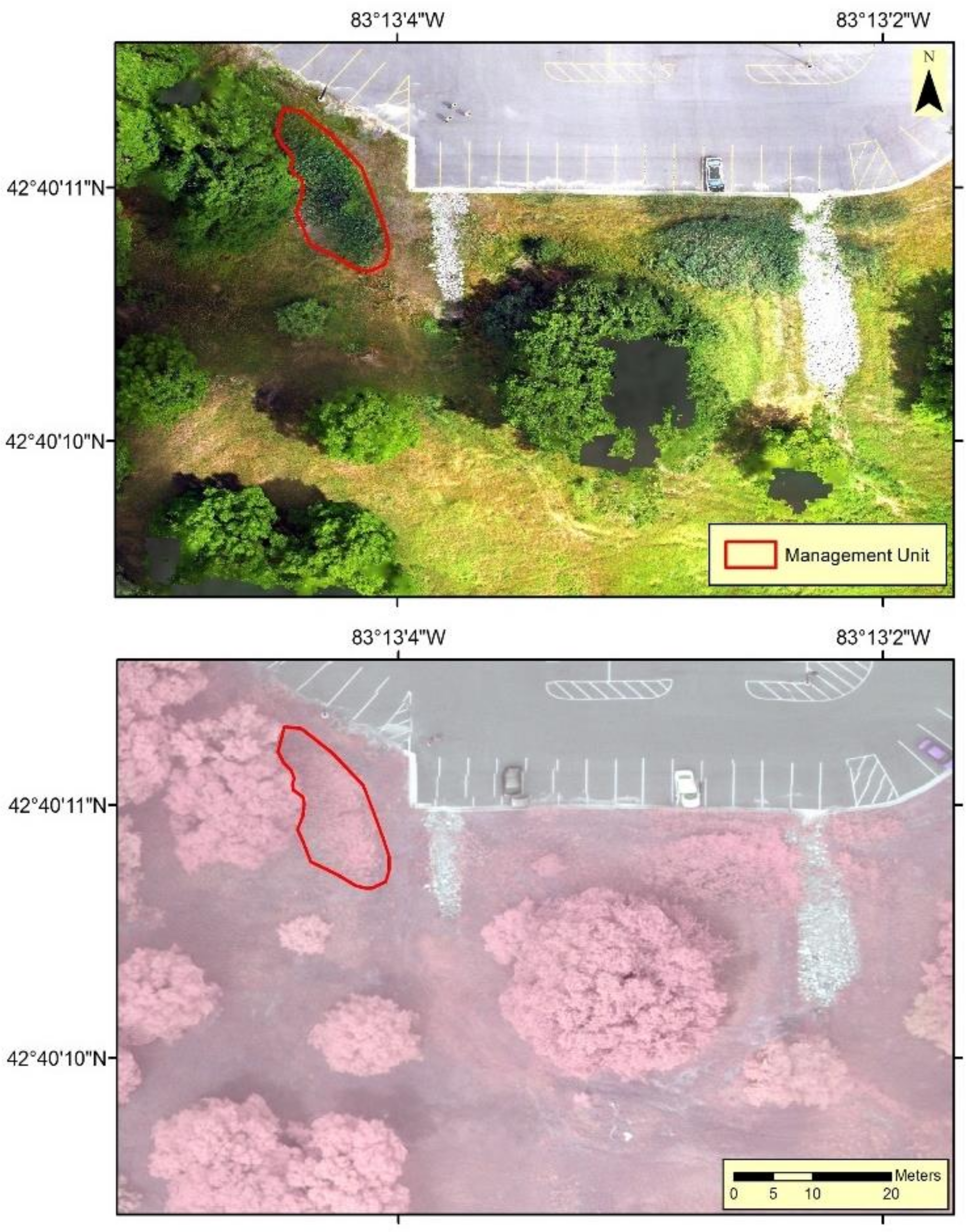
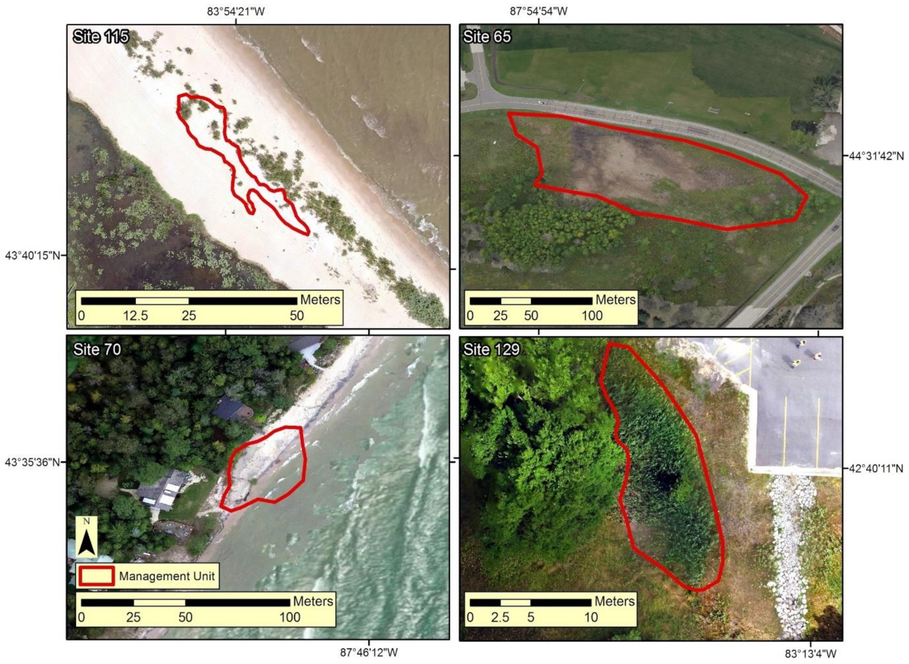
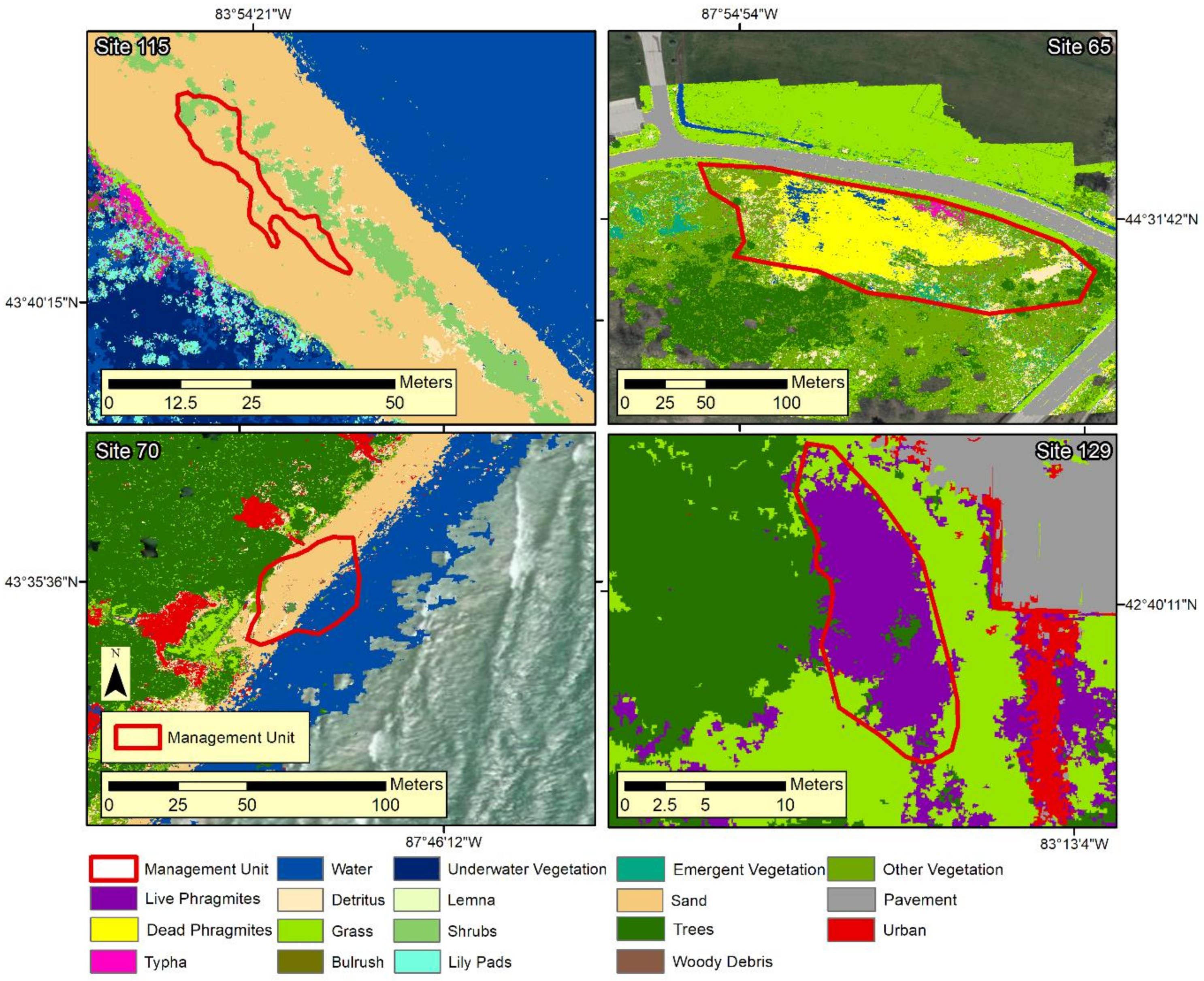
Figure 8 shows examples of four of the 20 PAMF sites, with the PAMF site boundaries as recorded by the PAMF program at the time of enrollment with the images being from the 2018 UAV data collection. Figure 9 shows the classification results for these same four sites.

Site 115 at the top left in Figure 9 is a site that had been covered by beach sand by the time of the 2018 UAV and field surveys due to higher Great Lakes lake levels. Site 70 (bottom left) is a site where beach retreat, due to higher like levels, had resulted in a PAMF site that was covered by sand and water in 2018. Site 65 (top right) is a site where PAMF treatment occurred and could be identified in the UAV imagery. Site 129 (bottom right) is a site where treatment had not occurred and live Phragmites was visible in the UAV imagery.

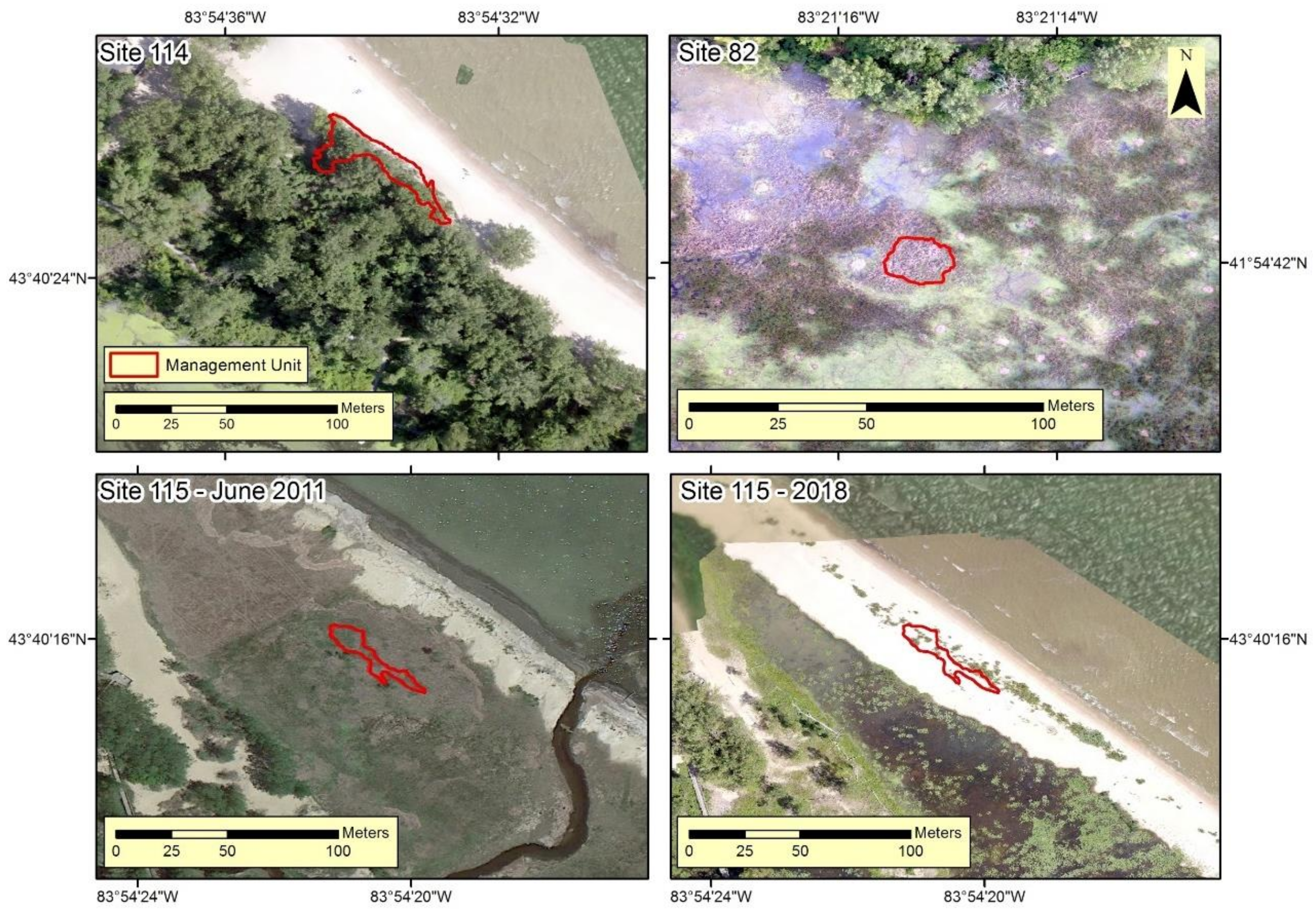
Figure 10 shows three sites where UAV deployment did not make sense for quantifying treatment areas. As noted, site 115 had been covered in sand sometime between the aerial photo taken in 2011 (bottom left in Figure 10) and this project’s 2018 UAV imagery (bottom right). Site 114 (top left) was under tree canopy, and Phragmites extent could not be identified. Site 82 (top right) is a very small area, less than 0.1 ha, that was probably too small to make UAV data collection necessary.

Using the four standardized classes, overall accuracy across all of the study sites was 91.7% and overall median accuracy was 92.6% (

Table 6. User’s and Producer’s accuracy metrics for each study site.

Standardized 4 Class Classification Accuracy Results			Live Phragmites User’s Accuracy	Live Phragmites Producer’s Accuracy	Dead Phragmites User’s Accuracy	Dead Phragmites Producer’s Accuracy
Site Number	Overall Accuracy	Area (ha)
59	100%	0.5	*	*	*	*
65	91.5%	0.9	*	*	100%	88.9%
69	100%	0.03	*	*	*	*
70	100%	0.07	*	*	*	*
71	100%	0.1	*	*	*	*
79	90.0%	0.2	*	*	50.0%	100%
80	78.3%	1.3	100%	66.7%	73.7%	100%
81	83.7%	2.2	100%	100%	*	*
82	Zero Samples	0.02	*	*	*	*
103	89.5%	0.5	50.0%	100%	66.7%	66.7%
104	100%	0.1	*	*	*	*
114	93.8%	0.05	*	*	*	*
115	100%	0.02	*	*	*	*
116	65.1%	5.4	100%	100%	*	*
117	88.1%	3.2	100%	75.0%	*	*
124	100%	0.1	*	*	*	*
129 (RGB)	85.7%	0.01	92.6%	92.6%	*	*
129 (NIR)	85.7%	0.01	89.7%	96.3%	*	*
132	83.3%	0.02	*	*	92.3%	70.6%
148	Zero Samples	0.08	*	*	*	*
151 (RGB)	100%	2.8	*	*	*	*
151 (NIR)	100%	2.8	*	*	*	*

* Classes that were not present in the classified image.

). The live Phragmites user’s accuracy was 90.3%, while the live Phragmites producer’s accuracy was 90.1%. We obtained a dead Phragmites user’s accuracy of 76.5% and a dead Phragmites producer’s accuracy of 85.23%. Where a category did not exist in the classification, we represent that with a “*” symbol (for example, site 65 only had “Dead Phragmites” present).

Grouping each classification into four specific classes worked well for the majority of our sites. Because the main interest of PAMF was to map the extent of live and dead Phragmites, additional vegetation classes were aggregated into a separate “other” (i.e., not Phragmites) vegetation class. In addition, by grouping other vegetation types into one category, our overall accuracy is more representative of both the live and dead Phragmites classes. Similarly, non-vegetation classes were also aggregated into another separate class.

Table 7. Summary of overall accuracies with and without using the NIR imagery for the two sites where NIR imagery was collected.

	Overall Accuracy without NIR	Overall Accuracy with NIR
Site 151	79.5%	81.8%
Site 129	85.7%	85.7%

summarizes the overall accuracy results obtained for the two sites where NIR imagery was available in addition to RGB imagery. The inclusion of additional spectral information from the NIR imagery that was collected at two of the study sites did not seem to significantly improve classification results. In site 151, overall classification accuracy improved from 79.5% to 81.8% when the NIR and NDVI data were included in the classification process; while in site 35, overall classification accuracy did not change with the additional data.

4. Discussion

The results of this study have demonstrated how UAV-based imaging and an object-based classification scheme can be an effective tool to measure the extent of dead and live Phragmites and other vegetation types at treatment sites, quantified within each management unit as total area and as percent cover. This method worked well overall, achieving overall classification accuracies >90%. These results are similar to other studies in the literature; Abeysinghe et al. [29] achieved 94.80% overall accuracy using a pixel-based neural network classifier and 86.92% overall accuracy using an object-based k-nearest neighbor classifier with multispectral UAV imagery and a canopy height model to map Phragmites in the Old Woman Creek estuary in northern Ohio. Conversely, Pande-Chhetri et al. [27] found that an object-based support vector machine classifier returned higher accuracy results than a pixel-based classifier for mapping wetland vegetation, although their overall accuracy was only 70.78%. Cohen and Lewis [30] also found success in using UAS imagery with a convolutional neural network classifier to map invasive Phragmites and glossy buckthorn (Frangula alnus) for ecological monitoring purposes. In their discussion, they recommend testing their methodology at a broader variety of sites. In this study, we tested a similar methodology across a broader geographical range of sites while still maintaining relatively high accuracy results. These results suggest that UAS imagery can be a useful tool for identifying the extent of Phragmites under a range of conditions, which can be useful for ecological monitoring. Such monitoring efforts could potentially see even higher accuracy with alternative machine learning classifiers such as neural networks and with repeated data collections at different phenological stages ([30]).

While our overall classification accuracy was relatively high, there were several sites included in the analysis that were not well suited for the use of UAV-based image classification. Management sites in forested areas could not be evaluated with UAV imagery due to the lack of visual penetration through tree canopy cover (Figure 10). Other sites, particularly those located on a coastline, were subject to hydrologic or geomorphologic changes that could artificially inflate or mask success metrics. For example, some sites that were noted as previously containing Phragmites were underwater at the time of measurement due to rising Great Lakes water levels, while another was located on a receding shoreline and eventually transitioned into almost entirely sand cover (Figure 10). Such areas might superficially be labelled as “successful” treatment sites, as there was a reduction in Phragmites cover after being enrolled in the PAMF program, but attributing this success to treatment would likely be inaccurate. In addition, some sites were also very small in size (less than 0.1 ha), making analysis of the area via UAV unnecessary to identify Phragmites presence and extent (Figure 10). These results suggest that there are ideal conditions in which UAV-based imaging for invasive species treatment monitoring is most effective. We suggest: (1) Treatment area extents must be visible from an aerial view (i.e., not under tree canopies); (2) Areas used to evaluate treatment efforts should not be drastically transformed by environmental factors prior to post-treatment image collection; and (3) The size and scale of the treatment area to be assessed with UAV-based imagery be larger than 0.1 ha. We also recommend that UAV flights take place before treatment, to establish a baseline, and after treatment was applied to compare how the area cover of the target species responded. These recommendations are more likely to help multiply the value of field data through use of UAV-enabled remote sensing.

At two sites (35 and 151), both NIR and RGB imagery were collected, which allowed us to assess the effects of classification accuracy with the addition of NIR. Using the standardized four class classification error assessment, the RGB and NIR imagery both provided equivalent results (site 35 with 85.7% accuracy and site 151 with 100% accuracy). When the validation was repeated for site 151 using the more detailed classification scheme (live and dead Phragmites, Typha, other live and dead vegetation, and trees/shrubs), the NIR imagery had 81.8% accuracy, while the RGB imagery had 79.5% accuracy. While these data may seem to potentially distinguish NIR imagery as providing improved classification results, the margin of success is not large and the site numbers are small. Using only these two sites for evaluation, the addition of NIR imagery into UAV based Phragmites classifications did not yield measurably superior results as compared with solely using standard RGB imagery for image classifications. The off-the-shelf Phantom 3 solution appeared to perform as well the NIR solution that required a custom mount. However, we suggest due to the small sample size in this study additional analysis be done to evaluate the usefulness of multispectral UAV-based imagery to monitor the treatment of Phragmites australis.

Recent research has shown the value of using NDVI from UAVs for identifying submerged aquatic vegetation (Brooks [15]) and for mapping the extent and biomass of Spartina alterniflora in the Sansha Bay (Zhou, Yang and Chen [20]). Brooks et al. [21] and Brooks [15] focused on identifying Myriophyllum spicatum (Eurasian watermilfoil or EWM) using spectral profiles, showing that a modified version of NDVI using a red edge band instead of NIR provided sufficient water penetration for mapping EWM extent. Testing the usefulness of the red edge for Phragmites identification should be investigated to see if this helps identify emergent wetland vegetation as well.

In our study, UAV image classification was performed using an object-based classifier. This process was performed by multiple image interpreters using a variety of classification rulesets (Table 4). Each ruleset was customized to fit the conditions of the treatment site. Although this process is effective, it can be time consuming and labor intensive. We believe that this process can be simplified by using techniques such as hierarchical classification, multi-resolution image segmentation, and transferable rulesets to assist image interpreters during the object-based classification process. Collection of additional UAV images of Phragmites australis treatment areas in the Great Lakes basin would aid in the creation of a standardized object-based classification protocol where site conditions are similar. Additionally, repeat collections of a treatment site would capture the seasonal variability of an area and potentially enable more general classification rulesets to be created.

5. Conclusions

Aerial imagery from small UAVs offers a robust option for standalone mapping as well as bridging the gap between quadrat-scale field measurements and lower resolution airborne sensors or readily available satellite imagery. Plot data are required to capture fine-scale heterogeneity in vegetation cover that, in the context of this study, may be important for detection of surviving Phragmites patches and secondary invaders for spot treatment as well as for evaluating management success related to restoration of native/desirable vegetation. Training or calibrating satellite remote sensing algorithms using field plot information requires extrapolating across spatial scales. The high resolution (with pixel sizes smaller than 10 cm) and multi-hectare coverage possible with UAV imagery could help fill this gap and make upscaling more robust. Similarly, this form of near-surface remote sensing could be used to interpret and validate time-series products derived from moderate-resolution satellite sensors by allowing frequent temporal sampling ([31]) even under cloud cover.

In this study, we found that RGB UAV imagery could be used to characterize the vegetation cover of sites that had been enrolled in a Phragmites management program, with overall accuracy results greater than 91%. Area of live Phragmites could be mapped with accuracies greater than 90%, and areas of dead (treated) Phragmites could be mapped with user accuracies greater than 76% and producer’s accuracies greater than 85%. These types of accuracy results are likely to be high enough so that UAV sensing can be a useful tool for use by wetland managers with wetland mapping needs. The technology is at a price point for practical adoption, can be deployed rapidly, and can produce data that can help the manager make a decision about management without extensive processing time required by other remote sensing techniques, such as airborne or satellite data collection. UAVs can make it easier to get sufficiently accurate presence and extent information for areas that may be difficult to get to, including areas that may need monitoring of post-treatment response. This technology has been demonstrated to be a useful tool that fills the gap between field data collection and large investments in fixed-wing or satellite platforms. This makes the results even more useful to managers whether they are federal professionals or landowners with varying levels of experience.

Aerial UAV-collected imagery provided a view that was more informative on Phragmites extent than field work alone. While we were able to map invasive Phragmites at a range of sites across the Great Lakes region, we found that the success of UAV-enabled monitoring depends on specific site characteristics, including that sites should not be too small (<0.1 ha), should not be obscured by tree cover, should have had active treatment occur that could be identified and measured with UAV imagery, and not be subject to changes that obscure potential treatment effects.