
Multi-Task Fusion Deep Learning Model for Short-Term Intersection Operation Performance Forecasting


MOT Key Laboratory of Transport Industry of Big Data Application Technologies for Comprehensive Transport, School of Traffic and Transportation, Beijing Jiaotong University, Beijing 100044, China
*
Author to whom correspondence should be addressed.
Remote Sens. 2021, 13(10), 1919; https://0-doi-org.brum.beds.ac.uk/10.3390/rs13101919
Submission received: 18 April 2021
/
Revised: 12 May 2021
/
Accepted: 13 May 2021
/
Published: 14 May 2021
(This article belongs to the Special Issue Traffic Assessment and Monitoring with Remote Sensing and Geospatial Modelling)
Abstract
:Urban road intersection bottleneck has become an important factor in causing traffic delay and restricting traffic efficiency. It is essential to explore the prediction of the operating performance at intersections in real-time and formulate corresponding strategies to alleviate intersection delay. However, because of the sophisticated intersection traffic condition, it is difficult to capture the intersection traffic Spatio-temporal features by the traditional data and prediction methods. The development of big data technology and the deep learning model provides us a good chance to address this challenge. Therefore, this paper proposes a multi-task fusion deep learning (MFDL) model based on massive floating car data to effectively predict the passing time and speed at intersections over different estimation time granularity. Moreover, the grid model and the fuzzy C-means (FCM) clustering method are developed to identify the intersection area and derive a set of key Spatio-temporal traffic parameters from floating car data. In order to validate the effectiveness of the proposed model, the floating car data from ten intersections of Beijing with a sampling rate of 3s are adopted for the training and test process. The experiment result shows that the MFDL model enables us to capture the Spatio-temporal and topology feature of the traffic state efficiently. Compared with the traditional prediction method, the proposed model has the best prediction performance. The interplay between these two targeted prediction variables can significantly improve prediction accuracy and efficiency. Thereby, this method predicts the intersection operation performance in real-time and can provide valuable insights for traffic managers to improve the intersection’s operation efficiency.
1. Introduction
Intersections are the sites of collection and turn of vehicles, which can easily be the bottlenecks of restricting the entire road network operation efficiency fully. Improving the traffic efficiency of intersections has always been the concern of transportation researchers and engineers. Short-term traffic forecasting of the intersection operation state can provide real-time traffic information, which is helpful for traffic managers to optimize signal control schemes to mitigating traffic delays.
The main traffic parameters of intersections, including the passing time, traffic speed and waiting time, etc., are used to detect the intersection’s operating performance. Among these parameters, the passing time and traffic speed can intuitively reflect the intersection’s overall operating performance [1]. With the development of traffic sensors, especially the emergence of mobile Internet, it is possible to extract traffic parameters from large-scale traffic data. The mobile sensors-equipped vehicles (i.e., the floating car) can monitor the traffic operation performance of large-scale intersection groups at low cost [2]. It can transfer the real-time traffic information to the database by the Global Positioning System (GPS) and modern communication technology, which have gradually become the mainstream approach to probe the intersection operation performance. The GPS is one of the Global Navigation Satellite System (GNSS), which can accurately locate the vehicle trajectory in real time [3]. The GPS system can track vehicle trajectory and collect traffic data, which usually contains temporal information (i.e., timestamps), spatial information (i.e., longitude and latitude) and speed information [4]. Meanwhile, we also consider the external factors that affect the intersection operation performance, such as weather conditions, temperature, wind speed and precipitation. Since bad weather conditions will affect the speed of vehicles, resulting in delays at intersections [5].
Nowadays, there are two methods to extract traffic parameters, including the digital-map-based [6,7] and grid-based methods [8]. Even though the digital-map-based method is a higher accuracy approach, it has two drawbacks: computational complexity and the high quality of the GIS Digital Map. Especially for the intersection, it is sometimes difficult to obtain a high-precision digital map to correspond to the more complex structures. Recently, we proposed an efficient grid-based method to visualize the signal intersections and evaluate the intersection operation state [9]. The grid-based method can discretize intersections into grids to improve the efficiency of extracting the traffic parameters. This efficient grid-based method is extended for the intersection. Moreover, based on the grid model, we can use the clustering method to identify the affected areas to explore the spatial traffic feature.
In the traffic prediction stage, the short-term traffic prediction development is based on the traditional statistical methods such as the Historical Average (HA), Autoregressive Integrated Moving Average (ARIMA) [10] and Kalman filter (KF) [11], etc. It is noted that the mathematical statistics-based methods have three main drawbacks: certain ideal assumptions, insufficient computing and massive multidimensional data. Primarily, it is inadequate to predict the complex real-time traffic state of intersections. With the development of computing technology, machine learning methods have made up for statistical defects. For instance, Support Vector Regression (SVR) [12], artificial neural networks (ANN) [13] are typical machine learning methods, which have been successfully applied to traffic flow forecasting. It is noted that the machine learning models above are difficult to deal with the large-scale Spatio-temporal traffic data.
With the development of intelligent technology, the deep learning method emerges as the times require. The typical time series model is the long short-term memory (LSTM) [14], which is evolved from the Recurrent Neural Networks (RNN) [15]. Compared with the RNN model, the LSTM has more advantages in processing long short-term time-series data, whose model structure is more advanced. Furthermore, Gated Recurrent Unit (GRU) model is a variant of the LSTM, which has a more concise structure and promotes faster convergence [16]. However, neither LSTM nor GRU model can capture the spatial traffic feature in intersections. In our previous research, we used the grid method to extract the spatial feature of floating car data in the expressway [16]. Noted that the intersection’s spatial traffic features are more complex, which is affected by travelers’ route choices and management control. In terms of spatial correlations, the convolutional neural networks (CNN) model is a mature method to extract spatial traffic features [17]. Even though the CNN model can extract intersections’ spatial features, the CNN model cannot reveal the intersection’s topology structure. The most plausible way to incorporate intersections topology into the deep learning model is to employ a graph convolutional neural network (GCN) [18,19]. Furthermore, to extract the Spatio-temporal traffic feature simultaneously, the fusion deep learning (FDL) models were proposed to predict the traffic Spatio-temporal state, such as the Convolutional LSTM Network (i.e., ConvLSTM) [20], CNN-LSTM fusion model [21] and GCN-GRU model [22]. Moreover, to distribute the weight of the FDL model reasonably, the attention mechanism is adopted to capture the corresponding weight of the MFDL model, which has been applied to short-term traffic prediction [23]. The ResNet has been applied to traffic prediction, such as the traffic flow predictions [24,25]. To our best knowledge, however, the ResNets rarely apply to predict the traffic performance of an intersection. Therefore, we combine the residual network with CNN model to extract the spatial features of intersections.
This research focuses on devising the multi-task fusion deep learning model (MFDL) to predict the intersection operation performance. The multi-task learning method has been applied in traffic fields such as network traffic classification [26], traffic flow forecasting [27] and traffic demand prediction [28]. Moreover, the multi-task learning method is rarely used in intersection prediction. The two main reasons are that the intersection’s traffic state is more complex and the high-precision data is not easy to obtain. This paper selects the passing time and speed as the prediction targets, which can reflect the process state and the visual state of the intersection. Compared with the existing multi-task model, we adopted the attention mechanism to assign the weight of variables to achieve feature fusion automatically. The multi-task learning method considers the difference between passing the time and speed and sharing each task’s common feature, which is a more comprehensive intersection operation state prediction. The contribution of this work is as follows.
First, based on the grid model, the traffic parameters are extracted. The grid-based method can identify the intersections rapidly without the digital map, which is easily transferred to other cities.
Second, the residual network (ResNet) is incorporated into the MFDL model to enhance the depth of the model, which contributes to alleviate the problem of gradient disappearance. Furthermore, based on the GCN model, the intersections’ topological propagation patterns are also considered, which previous studies were rarely involved.
Third, the MFDL framework integrates the deep learning method, preprocessed the data, extracts the traffic feature of the intersection, and finally predicts the passing time and speed of the intersections. Compared with the benchmark models, the MFDL model not only captures the Spatio-temporal traffic feature of intersections but also has better accuracy and robustness. Meanwhile, compared with the signal-task model, the MFDL can significantly improve the prediction accuracy and efficiency. The MFDL can be easily transferred to other cities for the traffic operation performance prediction of the intersection.
Using the intersection groups of Beijing as a case study, the proposed method’s accuracy and stability are demonstrated. The rest of this paper is organized as follows. Section 2 describes the floating car data and details the proposed methodology. Section 3 conducts a case study from the Beijing core area and an in-depth analysis of the experimental results. Finally, Section 4 ends with major conclusions and discussions for future research.
2. Methodology
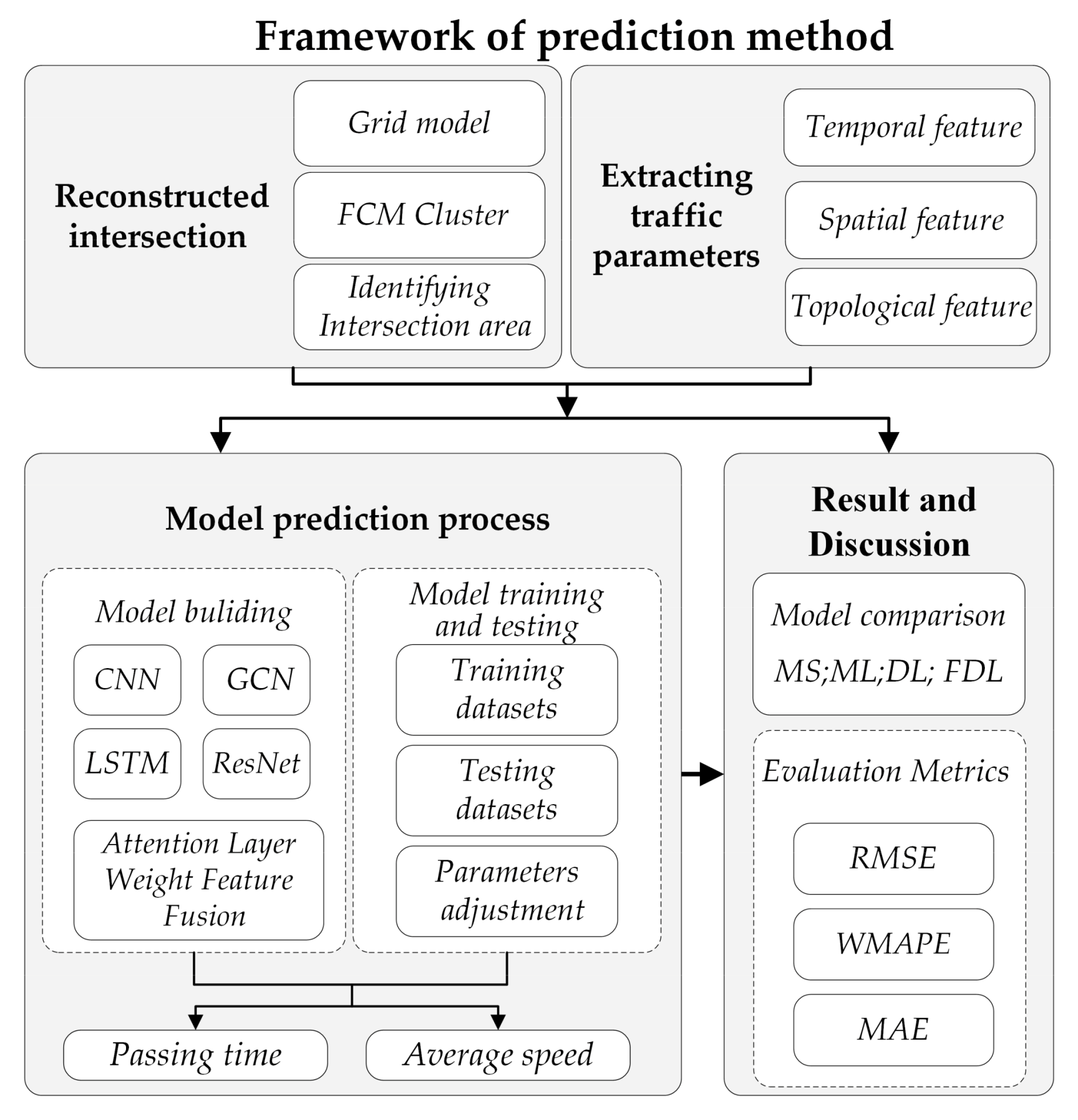
Figure 1 shows the multi-task fusion deep learning method framework, which includes the data process procedures, the model construct and model evaluation. For the first and second sections, according to the reconstructed intersection, the coordinate of floating car data (i.e., FCD) would be transformed to a based-grid coordinate to extract traffic parameters. For the third section, we construct the multi-task fusion deep learning model by fusing the CNN, GCN, LSTM and ResNet, an attention mechanism. For the fourth section, after entering the dataset into the model, we evaluate and verify the model’s effectiveness.
2.1. Data Preprocessing
The sampling rate of the obtained floating car data is 3 s, obtaining from DiDi company, one of the companies with the largest number of car Hailing users globally. The FCD data mainly contains three kinds of information: temporal, spatial and speed information. The variables and attributes of FCD are lists in Table 1.
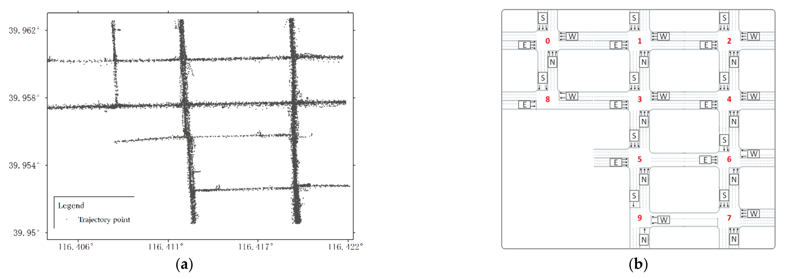
The data used in this case study include about 110 million floating cars’ trajectories, which the geographic coordinate ranges from 116.399450 to 116.431700 and the 39.947934 to 39.966344. The data are the same as those used in the previous study [9,29]. Figure 2a shows the trajectory points, and according to trajectories, we can obtain the topology of the intersection (see Figure 2b). We select ten intersections as the target objects in this study area, whose ID from No.0 to No.9 (see Figure 2b). The selected intersections cover three types, including the regular intersection with four legs (i.e., No.0 to No.7) and the intersection with three legs (i.e., No.8 and No.9).
Due to the block of GPS signal and the error of hardware/software in the process of data collection and transmission, there may be some errors in the original floating car data. It is necessary to preprocess the FCD to reduce the impact of error data and improve the prediction results accuracy. A more detailed data preprocessing process has been described in previous studies [9,16,29]. This paper introduces two main steps as follows:
Step 1: Remove the FCD, which is out of range of the intersection area; Delete the FCD whose speed is over 90 km/h; Eliminate the redundant FCD, which is similar or duplicate data.
Step 2: Replenish the missing data by the interpolation method due to the weak satellite signal or operation error during the FCD collecting.
2.2. The Grid Model
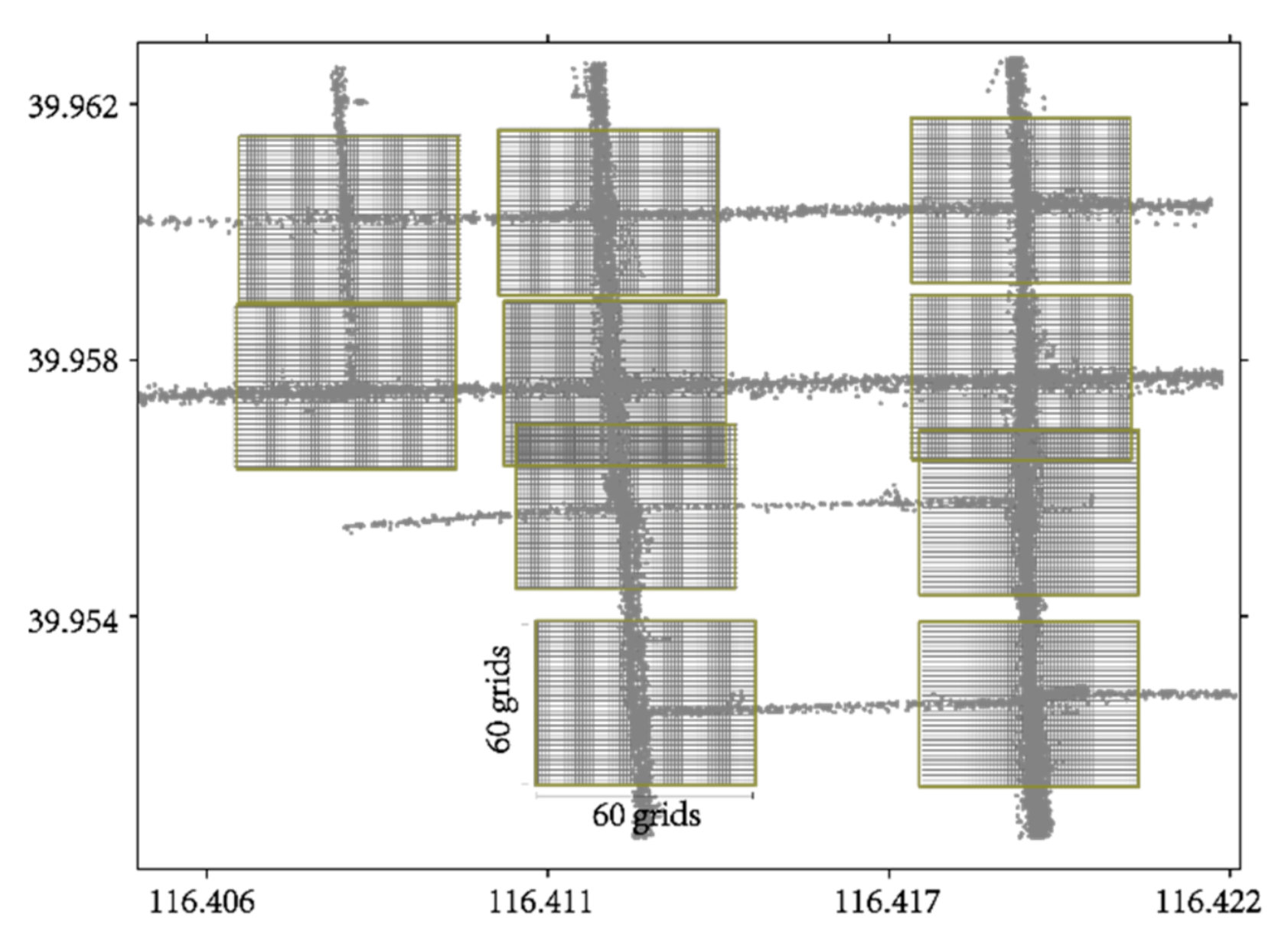
In this study, the intersection area range (i.e.,) is set to 300 m, covering the range of intersection proposed by the previous study [30]. In the intersection area, the intersection will be divided into discrete grids with a side length of ; If the grid size is too large, it may be out of the intersection area. Furthermore, if the grid size is too small, it cannot cover a floating car adequately. Previous study thought that the grid size of the identified intersection should be range from 1 to 10 m [31]. Given the above consideration, the length of the grid is set to 5 m, and the intersection area can be composed of , and the in this study (See Figure 3).
After dividing the intersection area into square grids, the floating car data is matched to the grid by the basic arithmetic algorithm, which is efficient and simple. Thereby, the FCD is transformed into the grid-based dataset (i.e., GFCD). Mathematically, the algorithm is as follows:
where are the right, left, up and down boundaries of the intersection area; are the number of rows and columns; is the grid coordinate that a trajectory point belongs to, whose latitude and longitude are .
2.2.1. Identification of Traffic Intersection Area
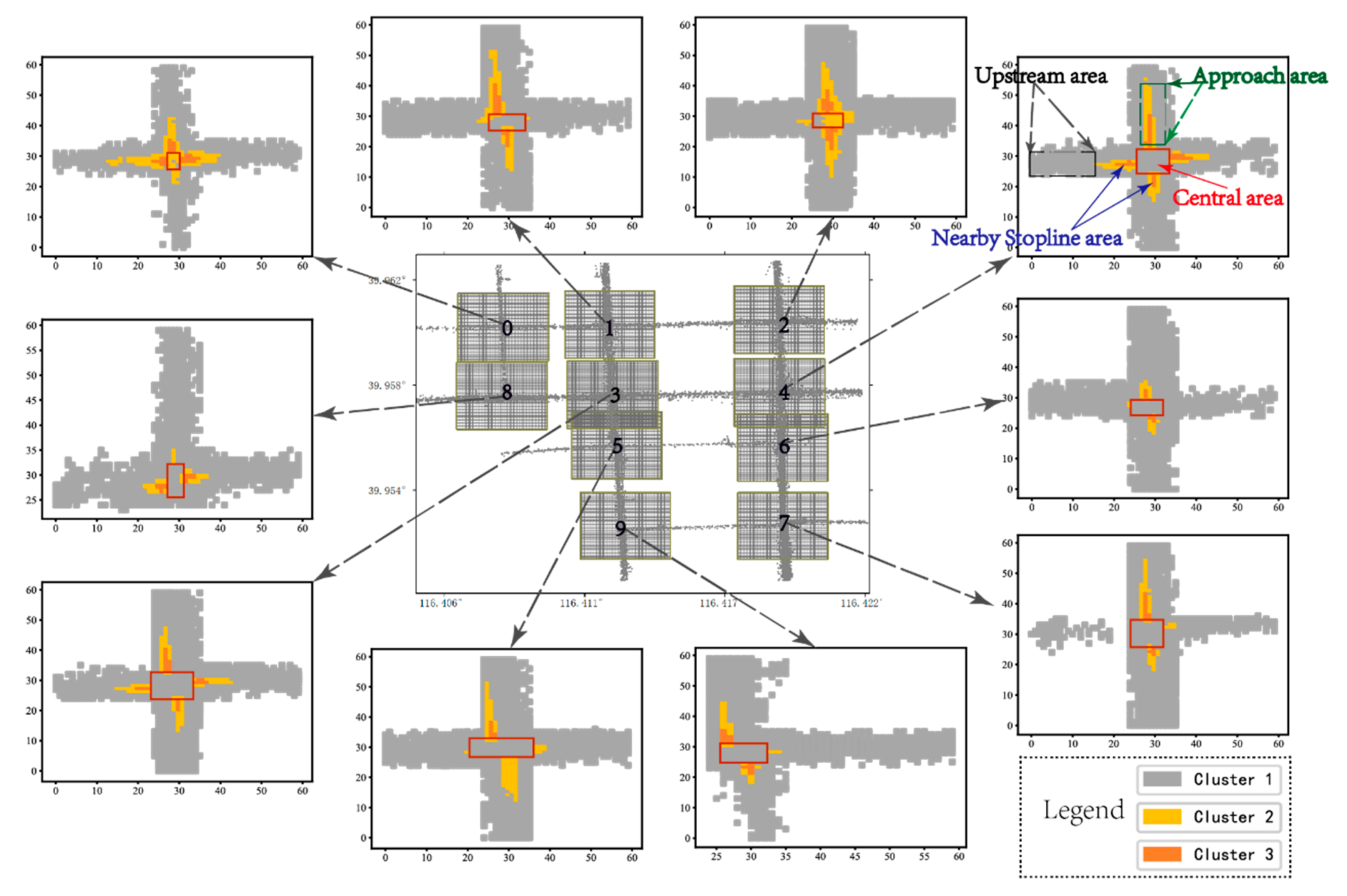
Due to the unique Spatio-temporal characteristics of each signalized intersection, the corresponding range of the influence area of signalized intersection is also different. If we define the influence area of signal intersection as a fixed area, it cannot sufficiently reflect the unique traffic characteristics of a signalized intersection. It is well known that the intersection is the bottleneck in the road network, where the stop-and-go phenomenon is also the most common. Therefore, we extracted the stop feature to define the range of the intersection. The stop frequency in a special area at intersections varies with the GFCD spatial feature. In general, the entrance area is more distinguished than other areas since the stop frequency in the entrance area is higher than the upstream and inner areas. Based on this feature, we constructed the stop dataset of GFCD by making statistics of stops in each intersection area grid.
Based on the stop dataset, the intersection area can be clustered into three groups, including the upstream area, the entrance area, and the nearby stop-line area. In order to distinguish the three areas, this study adopts the fuzzy C-means (FCM) clustering [32] method to identify the clusters. FCM clustering combines the essence of the fuzzy theory and provides more flexible clustering results [33]. In most cases, the traffic areas cannot be divided into obviously separated clusters. The membership degree of the FCM clustering method ranges from 0 to 1, which is suitable for the traffic stop scenario clustering. Based on the FCM, the function of FCM is as follow:
where is the membership degrees, which is restricted by the normalization rules (i.e., ), where is the number of GFCD and c is the number of cluster center; is the Euclidean Distance; is the spatial vector of GFCD; is the spatial vector of cluster centers;
Under the constraint , to minimize the objective function, it can be got through determining the derivation of Lagrangian. Then, iteratively update and by using the following equations:
According to the prior knowledge about the stop dataset, the number of clusters is set to three clusters: the low, medium and high frequency of stops corresponding to three areas (i.e., upstream, the entrance and nearby stop-line area). For the Beijing center area case, the intersection can be clustered into several groups (see Figure 4). Figure 4 presents the GFCD cluster result corresponding to the three areas, which shows the effectiveness of the proposed method. It intuitively can be seen that the cluster 1, 2 and 3 represent the upstream, entrance lane and nearby stop-line area. Moreover, the stop lines’ central area of intersections can be determined by the highest frequency of the stop. It is noted that the central areas of intersection 0 and 2 contain a part of cluster 2 since the left-turn phase is not set. This leads to the obvious conflict point between straight and turning left direction, leading to a high stop frequency in the central area. Furthermore, according to the different clustering results, we constructed the dataset of upstream, approach and central area of the intersection.
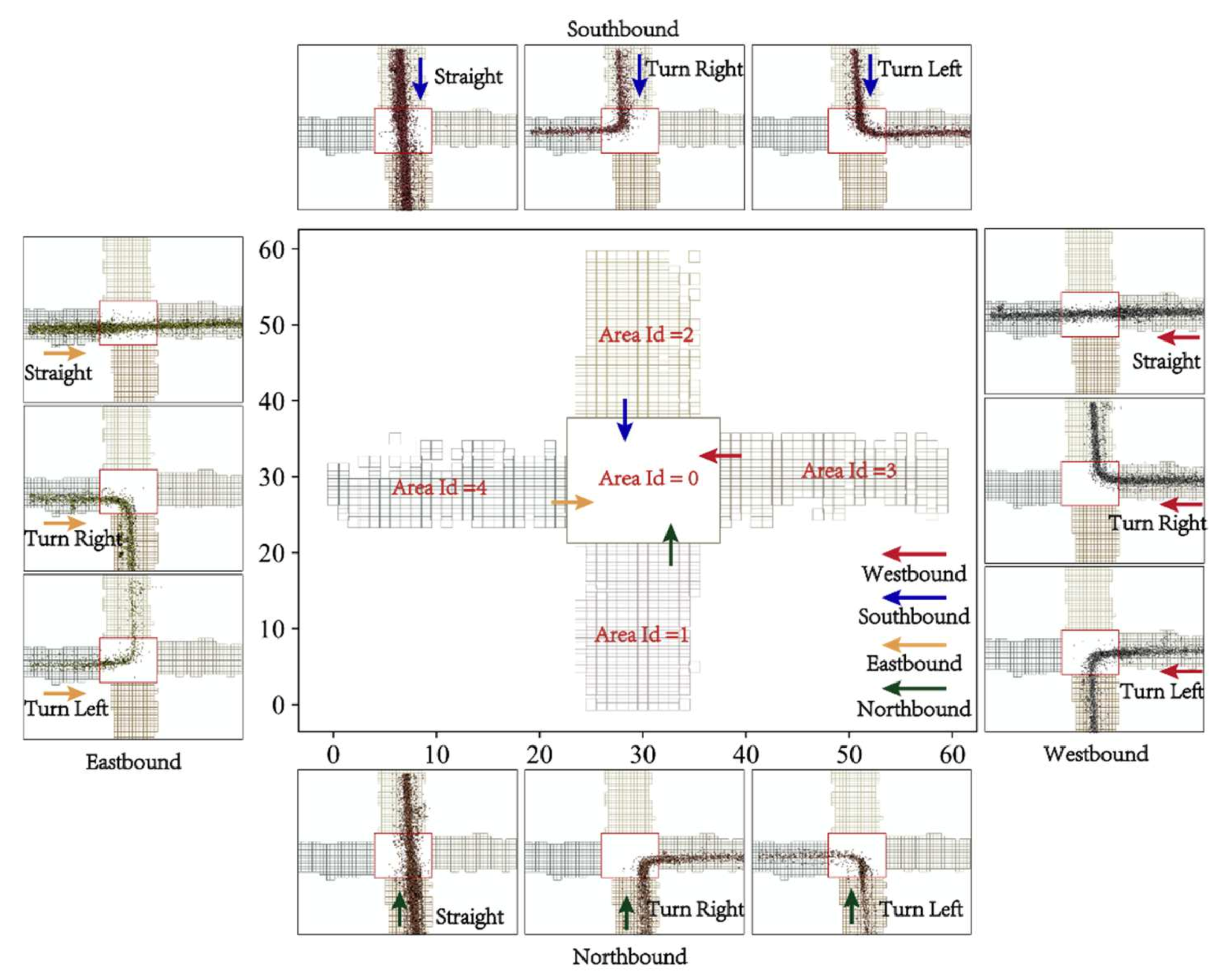
2.2.2. Identification of the Floating Car Trajectories Direction
After defining the intersection area range, the turning direction will be identified based on the grid model. First, the legs of the intersection are identified by GFCD and label (see Figure 5). The intersection legs can be divided into five areas, and the points of FCD are then mapped to the five areas. Then, based on the order of entering and exit Area ID, the direction of trajectory is identified, respectively. Taking southbound straight as an example, the entrance is 2 and the exit Area ID is 1, and it also passes through the central area of the intersection (i.e., ). Based on the grid model’s algorithm, it is simple to identify the direction of the floating cars’ trajectories passing through the intersection.
2.3. The Multi-Task Fusion Deep Learning Model
The multi-task fusion deep learning (MFDL) model architecture is composed of Residual Network, GCN, CNN, LSTM and Attention mechanism. Since the LSTM or the GRU only extracts the temporal information, the proposed model architecture can capture the Spatio-temporal feature and the topological structure of the intersection.
2.3.1. The Residual Network
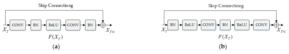
More road network features can be extracted by the deeper model [16]. However, the deeper models are easy to encounter the problem of gradient explosion and vanishing. To solve the problem, the Residual Network (i.e., ResNet) emerges as the times require [34], whose core idea makes the model deeper through the skip layer connection (see Figure 6a). The “Conv” indicates a convolutional layer, “BN” denotes a batch- normalization layer, and “ReLU” represents an activation layer. In this study, we use the improved structure of ResNet, which can solve the vanishing or exploding gradient problem better (see Figure 6b). The ResNet model is shown as follows:
where the is the residual block input; is the residual block output.
2.3.2. The GCN
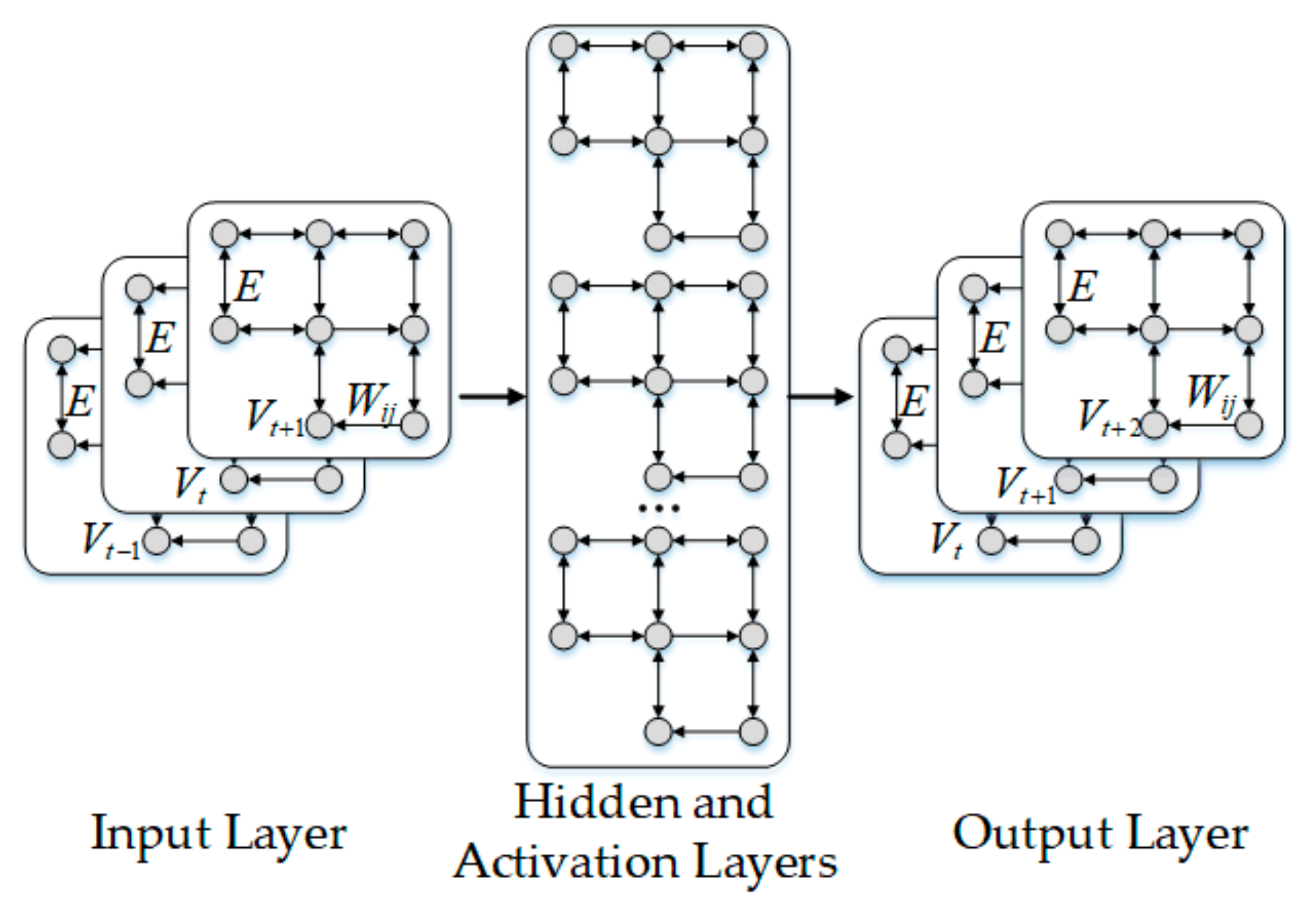
The road network can be regarded as a topological structure composed of points and lines, which points are intersections and lines are roads. When capturing the spatial feature, the CNN models cannot process the non-Euclidean structure’s data and extract the intersection’s topological relationship. In contrast, the Graph Convolutional Network (i.e., GCN) can make up for this defect [22]. It can capture the intersection of topological dependencies. In this study, the intersections are defined on the graph and focus on the structured traffic time series of pass intersection time (see Figure 7). At the time step , the intersections graph can be defined as . The observation is the set of vertices, corresponding to the observations from approaches in the intersections and the is the set of edges, indicating the connectedness between approaches in the intersections, while the is the weighted adjacency matrix of .
The GCN function can be defined as follows:
In Equation (8), is an activation function; , is the adjacency matrix, represents the identity matrix; denotes the diagonal node-degree matrix of ; the is the weight of the parameter matrix.
It should be noted that the calculation of stacking multiple GCN layers is more complex, and the gradient is easier to disappear [35]. Furthermore, with the deeper GCNs arising, the over-smoothing will make the features of the same vertex indistinguishable and debase the forecast accuracy [36]. Therefore, the ResNet GCN is proposed to make up for them. Then the graph signal of intersection is transformed to as the ResNet input. The has the same shape as the and the contains the topological information between the intersections.
In Equation (9), is the Laplacian matrix (see Equation (9); is the input; is the approaches of intersections; is the time steps for approaches in intersections.
2.3.3. Multi-Task Fusion Deep Learning Method
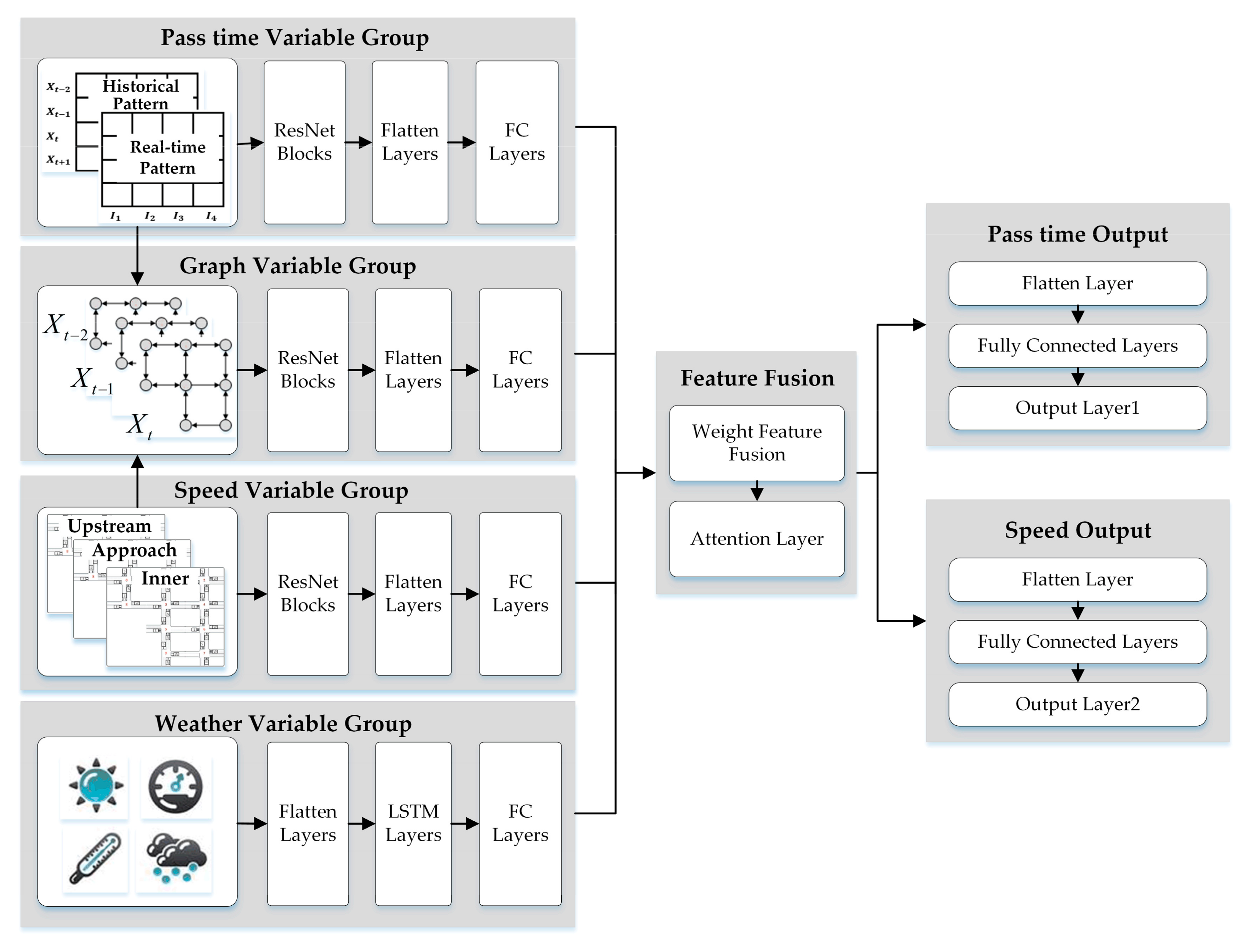
In this section, a novel multi-task fusion deep learning model framework is proposed to realize the intersection operation performance forecast. The framework integrates the historical pattern, real-time pattern, spatial pattern, topological structure and weather condition to predict the passing time and speed of the intersection. Herein, there are four variable groups in the multi-task fusion deep learning method (see Figure 8). In the first variable group, the passing time is used as the input variable to capture the temporal feature. The second variable group extracts the intersection topological information. The third variable group captures the Spatio-temporal features of speed. The fourth variable group shows that the effect of weather on prediction accuracy. The fusion section is used to fuse the information from four variable groups.
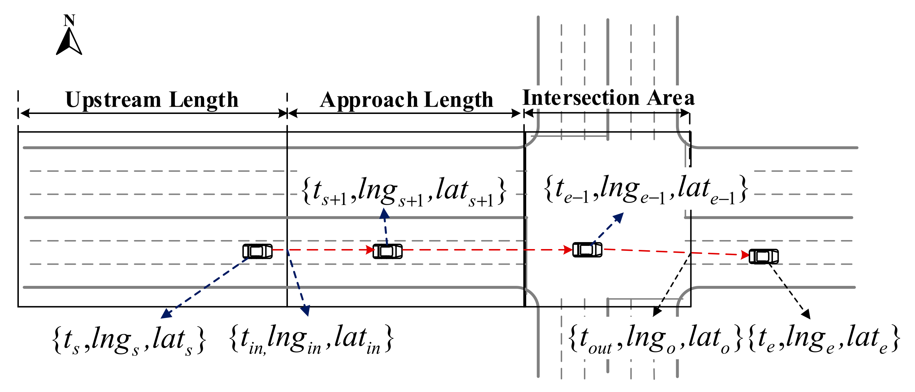
For the passing time variable group, the passing time is the most intuitive parameter representing the intersections’ operation performance [9]. Noted that the historical passing intersection time reveals the normal propagation rule and verifies the real-time passing time pattern. Therefore, this section adopts the historical and real-time pattern of passing intersection time as the input matrix. We extracted the passing time from the floating car data (see Figure 9).
According to the definition of intersection region effect, for intersection approach in different intersections, the trajectory’s passing time can be calculated by . Since the trajectory points do not coincide with the boundary of the intersection approach, it is necessary to estimate the time stamp of the approach boundary (i.e., ) based on the acceleration formula. In Equations (10) and (11), by calculating the distance (i.e., , R is the radius of the earth, | means or) between FCD point and the boundary of the intersection approach in geodetic coordinates, and combining with the time interval (i.e., Tin), we can obtain the time difference between the points and the boundary of the intersection approach. Therefore, according to Equations (10) and (11), the average passing time (i.e., ) can be calculated by Equation (12):
where the are the coordinates of the entrance and exit boundary of the intersection, respectively; are the coordinates of the trajectory points that enter and exit, respectively; represents the time interval, and the time interval of the floating car data in this study is 3 s.
The passing-time matrix is given by:
The input of the passing time variable group (i.e.,) is given by:
where is the number of entrances of intersections, and is the time steps for each entrance of intersections, presents the real-time pattern, presents historical patterns. In the passing time variable group, the three-time steps (i.e., ) are adopted to predict passing time. For example, when time granularity is 10 min, there are 96 time-slices in the daytime (i.e., from 6:00 to 22:00), and the dataset possesses 31 days of data. Therefore, for the 92 entrances lane at intersections, the input dimension matrix is [92 × 2 × 96 × 31]. The passing time matrix is divided into two datasets, the training dataset, whose proportion is 70% (i.e., [92 × 2 × 96 × 31 × 70%]), the test dataset, whose proportion is 30% (i.e., [92 × 2 × 96 × 31 × 30%]).
For the speed variable group, because of the spatial correlation between the upstream, inner areas and the entrance area, we selected three parameters: the upstream average , the inner average speed and the entrance speed as the input variables . The speed matrices ,, are defined as Equations (16)–(18). The input of the speed variable group (i.e., ) is given by Equation (19).
In the graph variable group, the intersection group’s topology has a great influence on the passing time. The ResNet GCN model is adopted to capture the topology of the intersection group. The passing time and average speed are input into the ResNet GCN model as the graph signal, respectively. According to Equations (9), (13) and (17), the graph variable can be defined as:
In the weather variable group, we consider four categories of weather variables, including temperature (i.e., TE, measured by Celsius degree), atmospheric pressure (i.e., PR, measured by Pascal), wind speed (i.e., WS, measured by a mile per hour) and precipitation (i.e., RA, measured by millimeter). The weather condition obtains one value per hour (see Table 2). The data is obtained from the free meteorological data website called “Wheat A” (Wheat A) [37]. To correspond to the time granularity of the average passing time, the time slice of weather-condition data should be transformed to the corresponding time bucket (e.g., the weather-condition from 6:00 to 6:10 will be equal to the recorded data from 6:00 to 7:00 (see the first row in Table 2). Similarly, according to the data division rules, the weather-condition data should be split into training and test dataset.
The input of the weather variable matrix is given by Equation (21).
In the feature fusion layer, the attention mechanism can distribute the different weights of the features from the neural network layers. In this paper, the attention layer is proposed to capture weight scores of different time steps, usually assigning a heavier weight score to adjacent time periods and a lower weight score to distant time periods [38].
where is a matrix consisting of output vectors , is the length of the vector. the , represents the feature variable from four subsection; are the weight of the different features; and the is the Hadamard product.
2.4. Model Configuration
The model experiment was implemented using Python 3.6 with Tensorflow [39], Keras [40] on Windows 10 for comparing the models. The experiment’s platform’s calculation cell is constructed with 32 CPU cores, 64G RAM and NVIDIA GeForce RTX 2080 GPU to meet the requirements of this experiment.
There are four subsections, the feature fusion and the output section, in the model framework. Moreover, the Rectified Linear Unit (ReLu) is used to solve the exploding/vanishing gradient problem. The dropout is set to 0.5 to prevent over-fitting. Furthermore, the Adam algorithm is proposed to update the parameters of the neural network. The partial hyper-parameter settings are shown in Table 3.
2.5. Models to Be Compared
This section will feed the training and test dataset to the proposed MFDL and benchmark models, respectively. Three typical benchmark models are selected to compare with the proposed MFDL model, including the mathematical statistics-based models (MS) (e.g., ARIMA), machine-learning-based model (ML) (e.g., SVR) and the deep learning model (DL) (e.g., LSTM, GRU, CNN and ConvLSTM). To ensure fairness, the following benchmark algorithms have the same input features (the same category and the time interval).
MS model: For the ARIMA model, we use the Akaike Information Criterion (AIC) as the standard to select the optimal model. Noted that it is difficult for the ARIMA model to capture the Spatio-temporal feature of the intersections, so we constructed 92 models to represent the 92 intersection entrance lanes.
ML model: Two main parameters selection of SVR (i.e., the penalty coefficient “C” and the parameter “Gamma”) are based on the cross-validation, and the kernel function is set to the radial basis function.
DL model: For LSTM and GRU both have two hidden layers and 128-unit neurons. For the CNN and ConvLSTM, the kernel size is 2 × 2, and the kernel layers are set to 32 and 64 filters, respectively.
MFDL model: We consider four models: the MFDL without weather (i.e., No weather), the MFDL without graph information (i.e., No Graph), the MFDL without CNN (i.e., No CNN), and the MFDL model.
The time lag is set to 10 min, and the hyperparameters are set the same as the proposed model. Then we use the RMSE and MAE to measure the total predictive accuracy of fitting in the whole test data and use WMAPE to measure the models’ predictive performance.
2.6. Loss Function and Evaluation Metrics
In order to compare the proposed fusion deep learning model framework with the benchmark models, three indicators are required to evaluate model performance, including the Mean Absolute Error (MAE), the Root-Mean-Square Error (RMSE) and weighted-mean-absolute-percentage error (WMAPE). The mean-squared error (MSE) is adopted as the loss function of speed and the passing time. Furthermore, the weight of loss is set to 0.5. These definitions are as follows:
where n is the number of test samples; is the real values; is the predicted values; is the average values.
3. Result and Analysis
3.1. The Spatio-Temporal Patterns of the Intersection
Figure 10 shows the average daily order volume of floating cars at ten intersections. It can be found intuitively that the order volume on the weekdays is larger than on the weekend, which means that the traffic pattern on weekdays is different from that on weekends. Meanwhile, the order volume of the ten intersections of different periods is different. It means that the traffic Spatio-temporal pattern of different intersections is different.
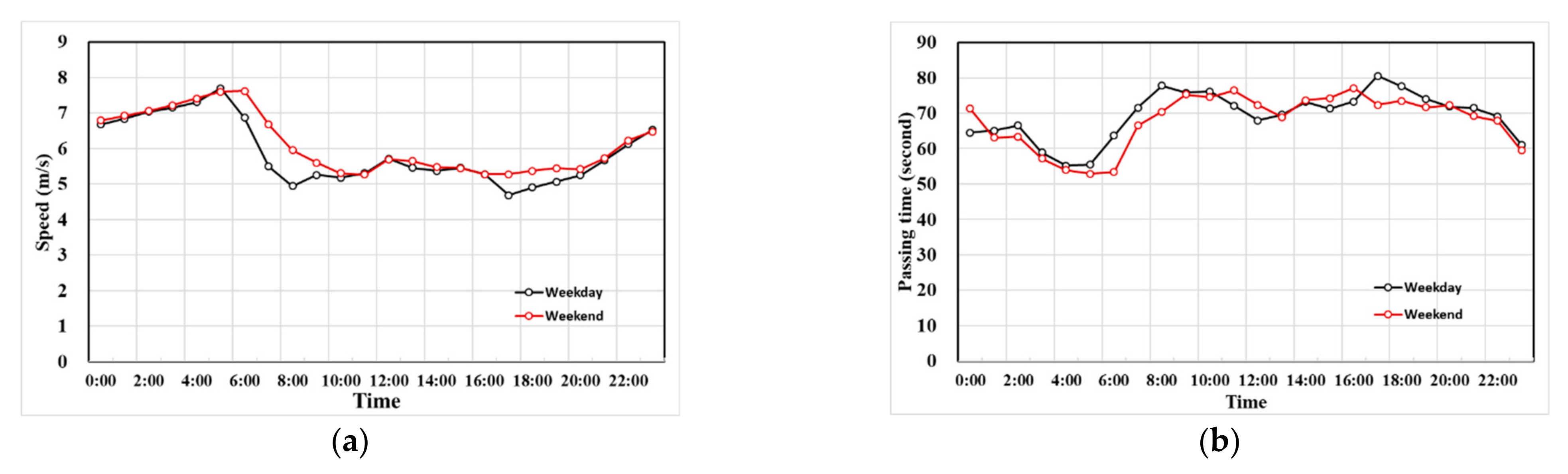
Figure 11 shows the trends of the average speed and passing time on both weekdays and weekends, respectively. It can be seen that the tendencies of the two-variables fluctuation are constant in the evening (0:00–5:00) both on the weekday and weekend. Therefore, when exploring the variables feature, we choose the daytime (6:00–22:00). Meanwhile, during the peak hours (i.e., 6:00–9:00, and 17:00–20:00), the speed tendency on the weekend is faster than the weekday in general. Corresponding to the speed tendency, the passing time on the weekday is longer than the weekend, meaning that the variables’ temporal features are discrepancies. Therefore, it is necessary to consider the temporal characteristics in the prediction experiment.
3.2. The Correlation between Speed and the Passing Time
The passing time can directly represent the operation performance of a signalized intersection, and the speed can directly reflect the visual state of the intersection operation state. It is necessary to carry out a correlation analysis between the passing time and the speed to enhance the interpretability of the model and improve the accuracy of the model [41]. The Pearson correlation coefficient can reflect the correlation degree of the two variables, which range from −1 to 1 [42]. Suppose the correlation degree is greater than zero, which indicates that two variables are positively correlated. In that case, that is, the greater the value of one variable, the greater the value of the other variable. If the correlation degree is small than zero, which is means that the two variables are negative correlation; that is, the larger the value of one variable is, the smaller the value of the other variable.
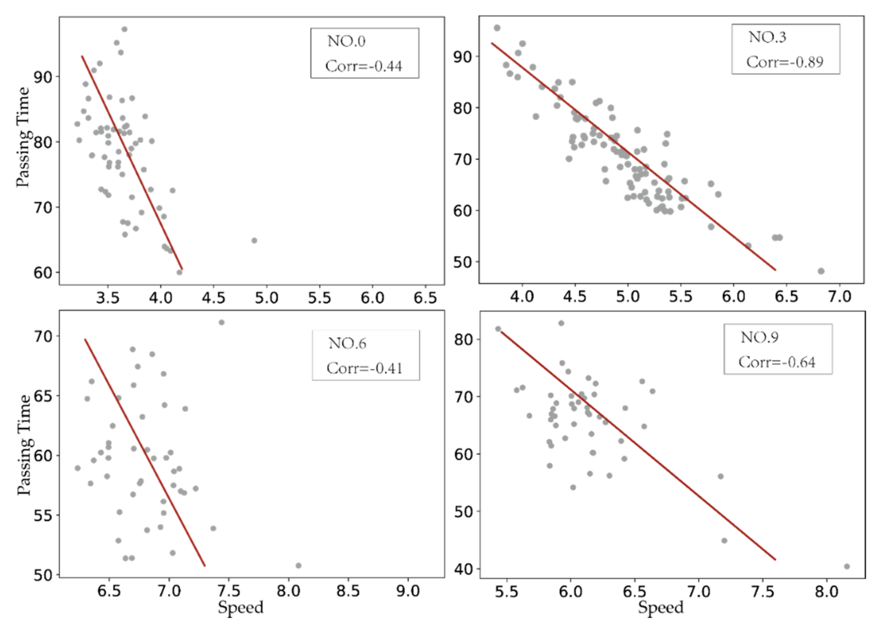
The total correlation degree between the average speed and the passing time is −0.84, which means that the two variables are a strong negative correlation. Moreover, we select four typical intersections, including the No.0 with fewer orders, the No.6 with a one-way lane, the No.9 with three legs and the regular No.3 (see Figure 12). It can be seen that the absolute value of correlation degree of No.3 is the largest (i.e., −0.89), and due to the influence of intersection topology and signal phase, the correlation degree of other intersections decreases.
3.3. Model Performance Comparisons and Result Analysis
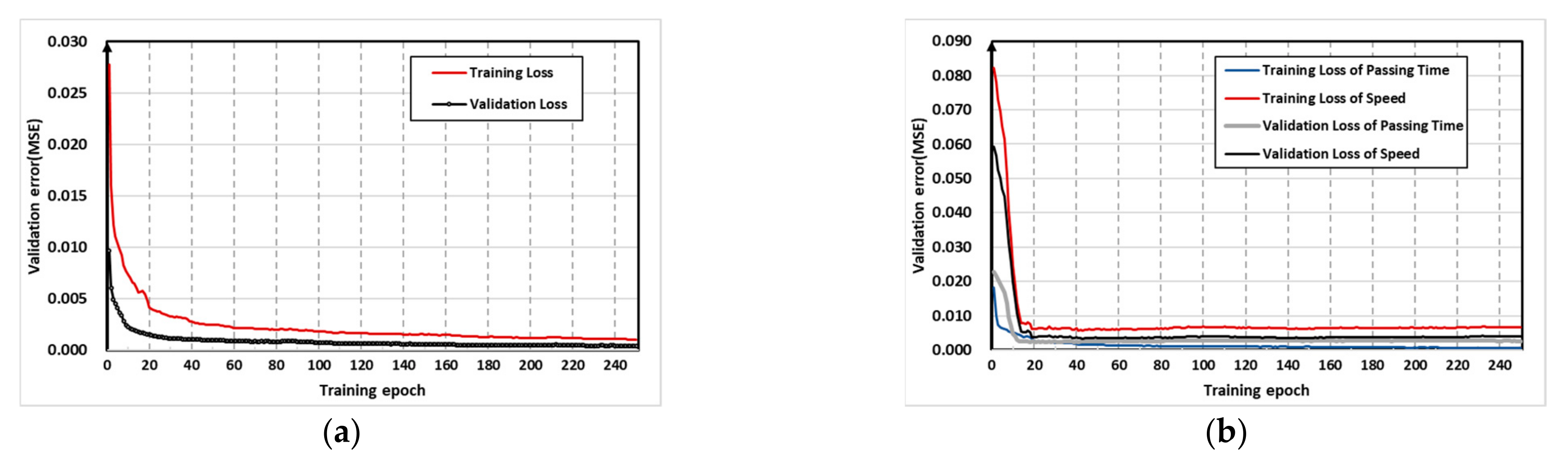
Figure 13 shows that the training procedure, to training the optimal model and avoid the overfitting problem, the early stopping technique is proposed. It can be seen that the training and validation loss decrease rapidly. Furthermore, the training and validation loss has remained stable in 50 epochs, which means that the proposed model’s robustness is strong.
The prediction performances are shown in Table 4. As shown in Table 4, the MFDL considerably outperforms mathematical statistics-based and machine-learning-based models in most cases. The ARIMA model has the worst performance since the ARIMA lacks capturing the spatial feature of traffic parameters and processing the complicated nonlinear problems. Moreover, the SVR also has poor performance. It is difficult for SVR to deal with large-scale Spatio-temporal data when it consumes limited computing resources.
Compare with the MS and ML models, the deep learning models perform better. Through the control method of input, activation, and output of traffic data flow, continuously circulate iteration, the deep learning model can better capture a large-scale time series’ characteristics. Among the deep learning models, the Conv-LSTM has the best performance since the Conv-LSTM can capture the temporal information and the spatial information.
The experimental results illustrate that the multi-task fusion deep learning models work best among these methods, which can efficiently learn the Spatio-temporal feature of the two targets’ predicted variables. As Table 4 shows, taking the prediction speed and the passing time in 10 min time granularity as an example, the MFDL model outperforms the MS model on RMSE, MAE and WAPE with the improved accuracy of 1.94, 1.34, 14.47%, 15.01, 14.04 and 23.63%, respectively. This is because the MFDL models contain the characteristics of time series, space, topology and weather. It is noted that the MFDL model is less affected by the weather, and the prediction accuracy is not significantly affected when the weather subsection is deleted. In contrast, the No-CNN model result (i.e., the MFDL without graph) changed more significantly, although the No-CNN model reveals better performance to capture the intersection’s topology dealing with the temporal feature with low ability.
In general, with the increase of the time granularity (Tg), the prediction performance gets worse. This phenomenon is due to the larger the time granularity, the smaller the data sample. In addition, all of the speed metrics values are smaller than the passing time since the passing time’s random fluctuations at different intersections have a more significant disturbance.
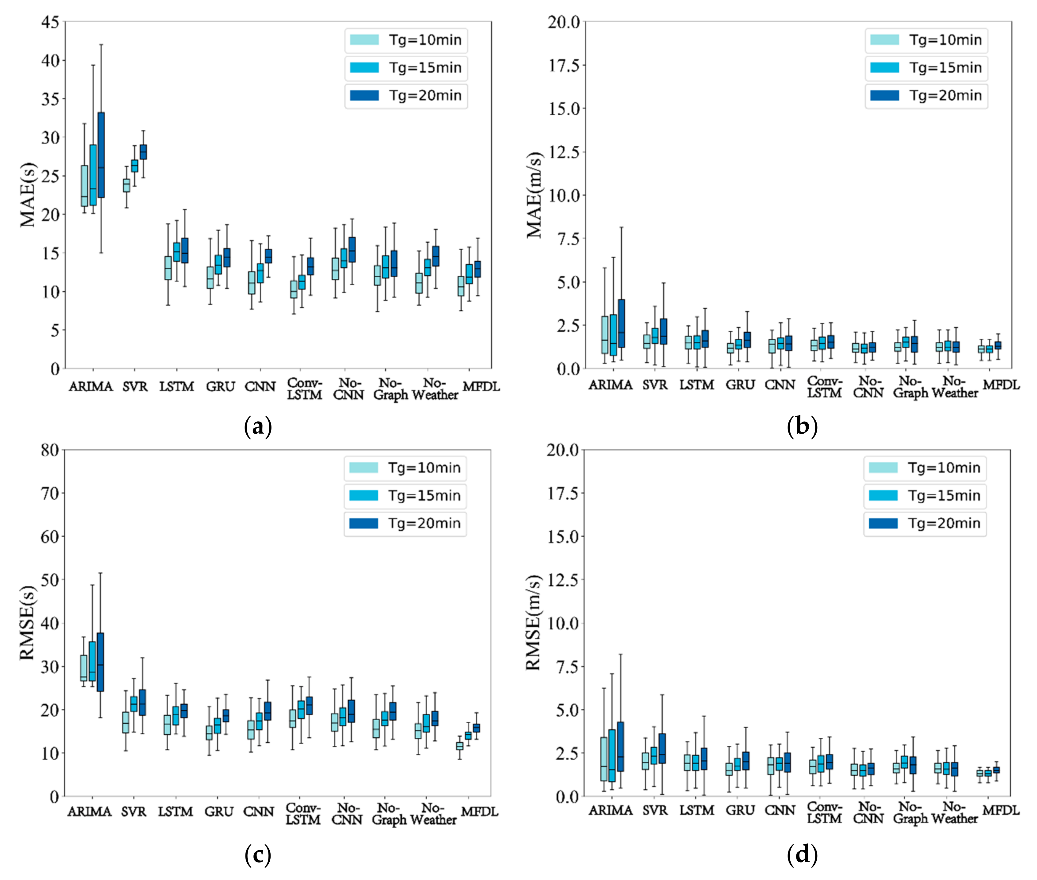
Figure 14 shows the overall prediction errors produced by the different methods on different time granularities (i.e., Tg = 10, 15 and 20). It intuitively indicates that the proposed model reveals the best performance on the passing time and speed among the benchmark models. In contrast, the ARIMA model has the most significant error dispersion, which indicates that the ARIMA model cannot regress the multi-task Spatio-temporal feature. Furthermore, it can be seen that the MFDL model has a smaller interquartile range, whose distance between Quartile 1 and 3 is smaller, and the metrics values are more concentrated than other models. Moreover, with the increase of time granularity, the error distribution becomes more dispersed, which revealed the results mentioned in Table 4.
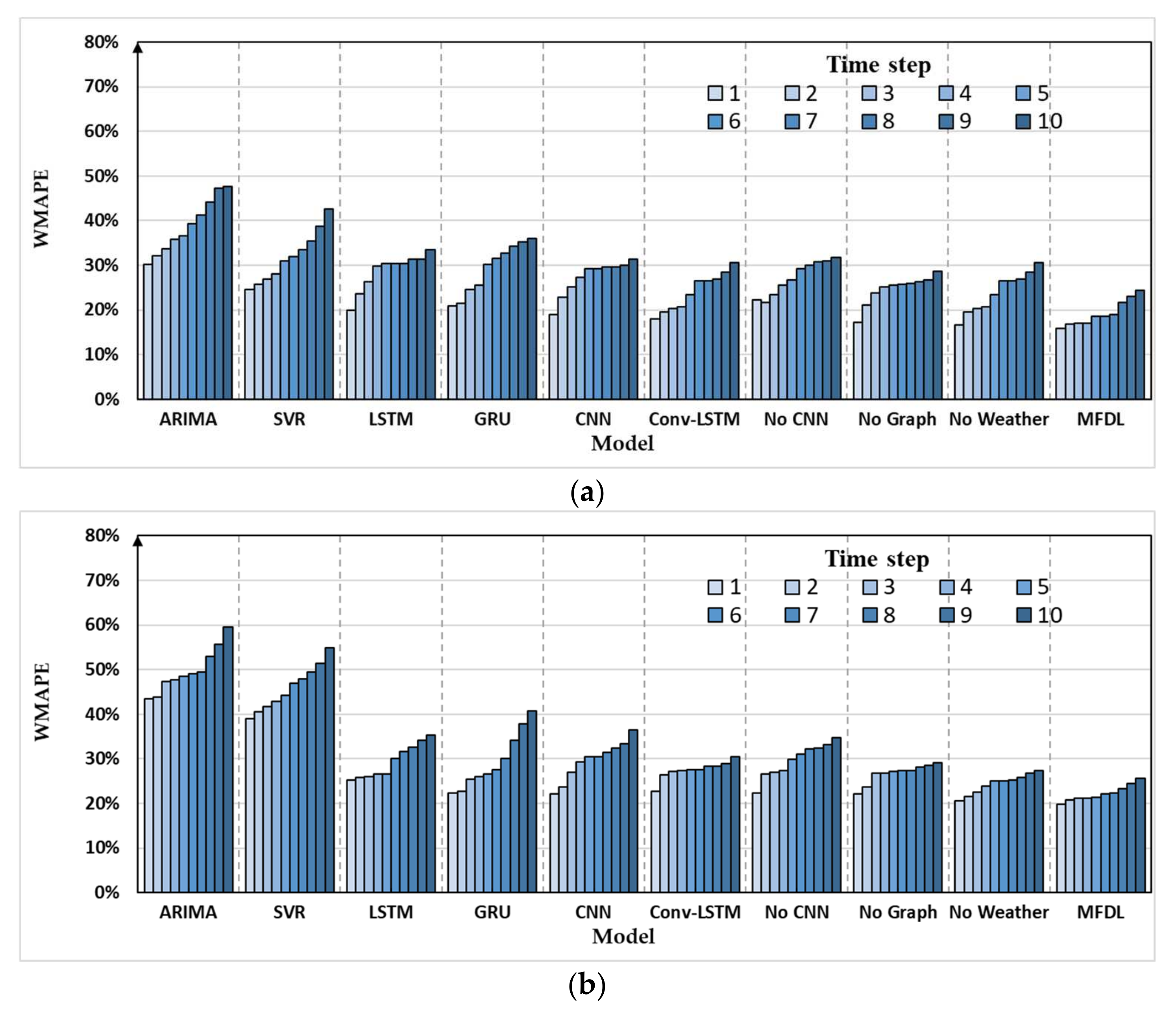
Figure 15 demonstrates the comparison of the benchmark model and the proposed model in terms of various time steps by WMAPE. As shown in Figure 15, the ARIMA and SVR models work worst in different time steps. In contrast, the proposed MFDL model can provide reliable prediction precision, which the WMAPE is the lowest among the models in different time steps. Furthermore, as the increase of time step, the increase of the metrics of the MFDL is the least, indicating the stability of the MFDL model is excellent.
Table 5 shows the comparison of individual prediction metrics and multi-task prediction in 50 epochs. It can be seen that the prediction precision of the passing time and speed in multi-task fusion deep learning (MFDL) is better than the prediction of the passing time and speed in single-task learning (STL) in different time granularity. This phenomenon indicates that the passing time and speed can promote each other to improve the prediction accuracy. In addition, the training time in the STL model consumes more time than the MFDL model in 50 epochs. It is noted that when the time granularity is 10 min, the training time is reduced by 8.3 min and the efficiency increases by 46.42%, which means that the MFDL is more efficient.
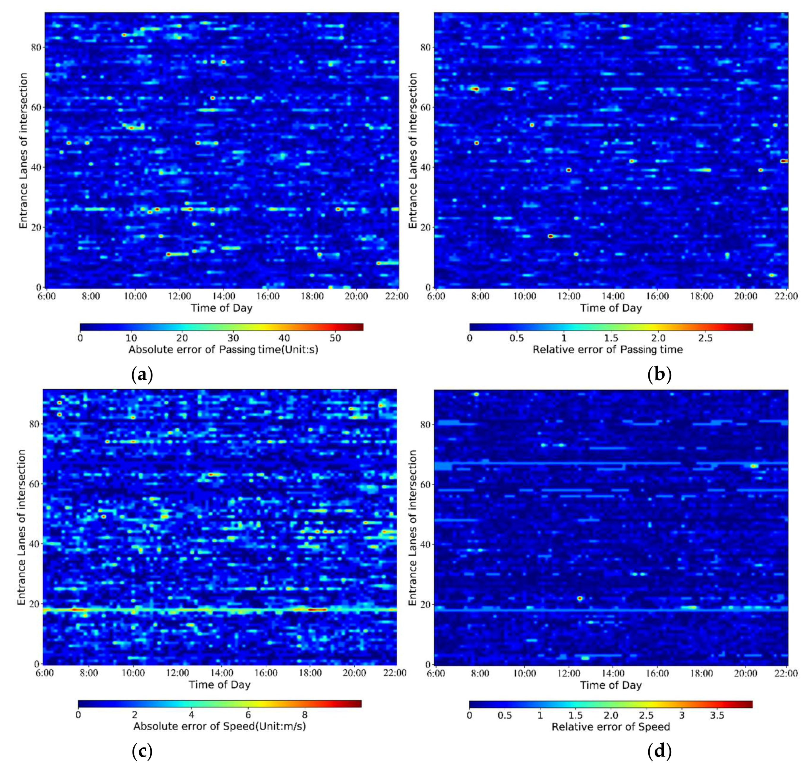
Figure 16 shows the heat maps of the absolute error (i.e., ) of average speed and the passing time and the relative error (i.e., ) of average speed and the passing time at the intersection entrance lane in a one-time step by MFDL. The x-axis represents the time of daytime (from 6:00 to 22:00), and the y-axis represents the 92 entrance lanes of the intersection. In Figure 16, the deeper the red color areas are, the more significant the errors are, and the deeper the blue color areas are, the lower the errors are.
From Figure 16a, it can be seen that most of the passing-time absolute errors are below 10 s. Minority entrance lanes have a slightly higher absolute error at a specific time. Noted that although the absolute delay of some entrances is significant, the relative error is small (see Figure 16b). For example, the absolute error on the entrance 26 (i.e., northbound left-turn entrance lane of intersection No.2) is significant during 7:50 to 8:40, 12:10 to 12:30 and 19:10 to 19:20, etc. However, the relative error of entrance 26 is inconspicuous. This phenomenon is probably due to the average passing time of entrance 26 is longer (i.e., 141 s) than the average passing time (i.e., 69.4 s) in intersection 2, which has more interference factors leading to absolute error.
From Figure 16c,d, it can be intuitively seen that there is a significant difference between the pattern of relative error and the pattern of absolute error of speed. Even though some of the speed absolute errors of some entrance lanes are significant, the relative errors are minor. Since the average speed is smaller (i.e., 7.78 m/s), the relative error of speed is more sensitive to the ground-true speed, which may lead to a larger relative error. Taking the entrance lane 18 (i.e., southbound right-turn of intersection 1) as an example, the absolute error and the relative error are significant, indicating that data fluctuation is volatile, affecting prediction accuracy.
Overall, the MFDL model can primarily capture the Spatio-temporal characteristics of the passing time and traffic speed in the intersections and make an accurate prediction. The prediction error visualization can significantly express the accuracy of prediction results.
3.4. Sensitivity Analysis
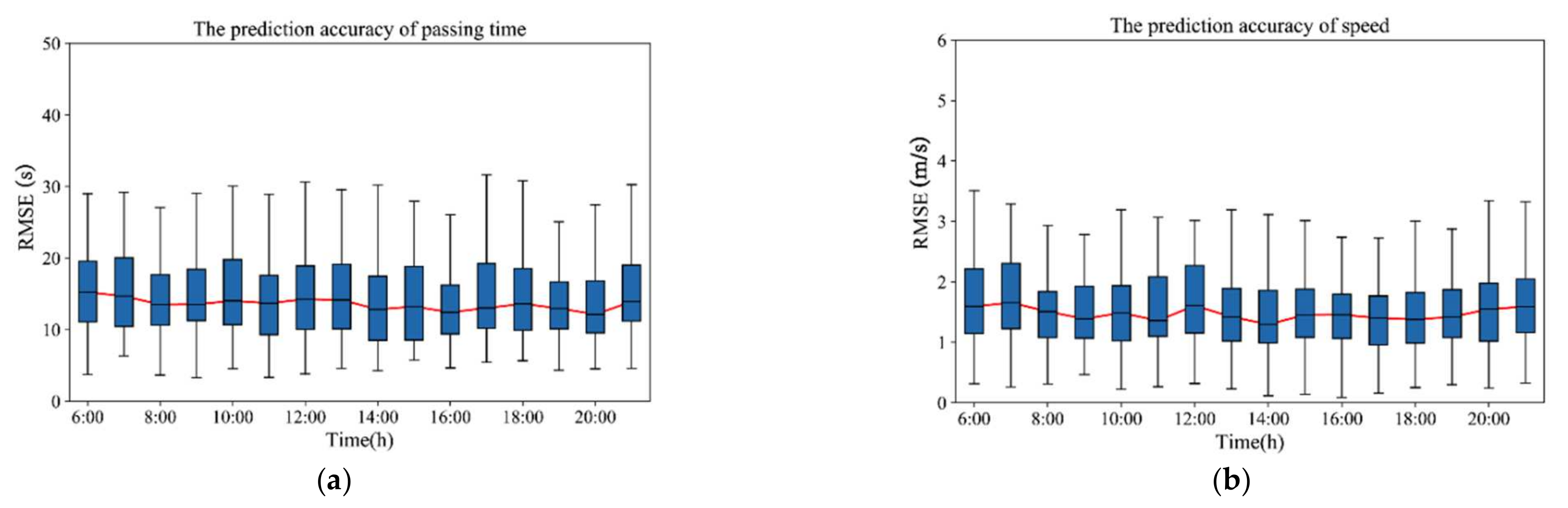
For the MFDL models, the temporal features of inputs are likely to be associated with the accuracy and stability of the prediction result, and we select the RMSE as the evaluation index. Figure 17 shows the RMSEs of the passing time and speed. The red curve means the fluctuation trend of the RMSE median, and the blue box pattern represents the error distribution of 92 entrance lanes in different periods. It can be seen that the RMSEs of the MDFL model fluctuate slightly throughout the day, indicating that the MFDL model has strong robustness. Moreover, the RMSEs fluctuate of the passing time rise slightly during the peak hour (i.e., 7:00–8:00, 17:00–18:00), whose median only increases by 2.4 of an entire day. Meanwhile, the RMSEs fluctuate in the speed prediction is also relatively low. In conclusion, the proposed model has high accuracy and fine stability under various temporal features.
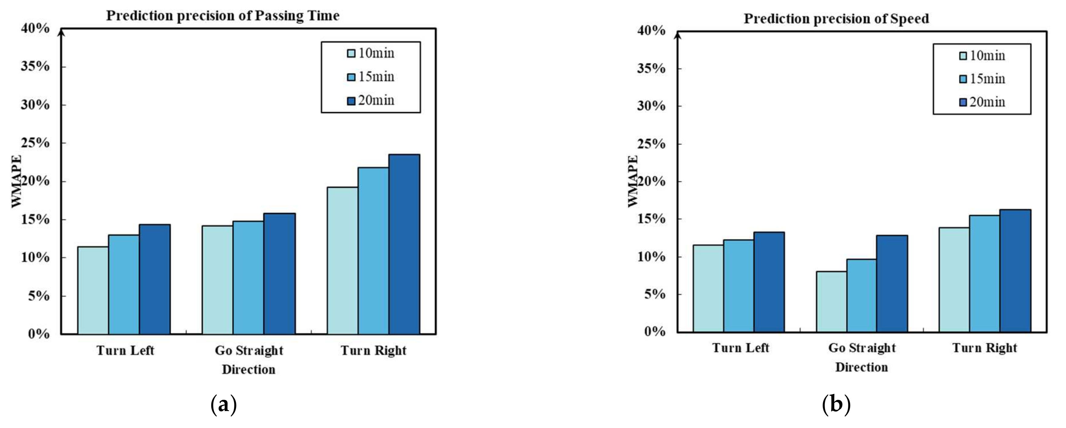
Furthermore, the spatial features of input may be associated with the accuracy of the prediction result. Since it is not significant to build a GCN model only for a single direction prediction experiment. Therefore, we carry out the experiment by the MFDL-No-Graph model. Figure 18 shows the result of the evaluation metric (WMAPE) of different time slices in different directions. It can be seen that the WMAPE in different directions is different. The floating data fluctuates in various spatial positions, which influences the prediction results. Obviously, the WMAPE of the turn-right direction is significant due to the turn-right data having more interference factors (i.e., non-motor vehicles and pedestrians), leading to more data fluctuates. Moreover, the WMAPEs increase with the time granularity, which implies that the more samples, the higher prediction accuracy.
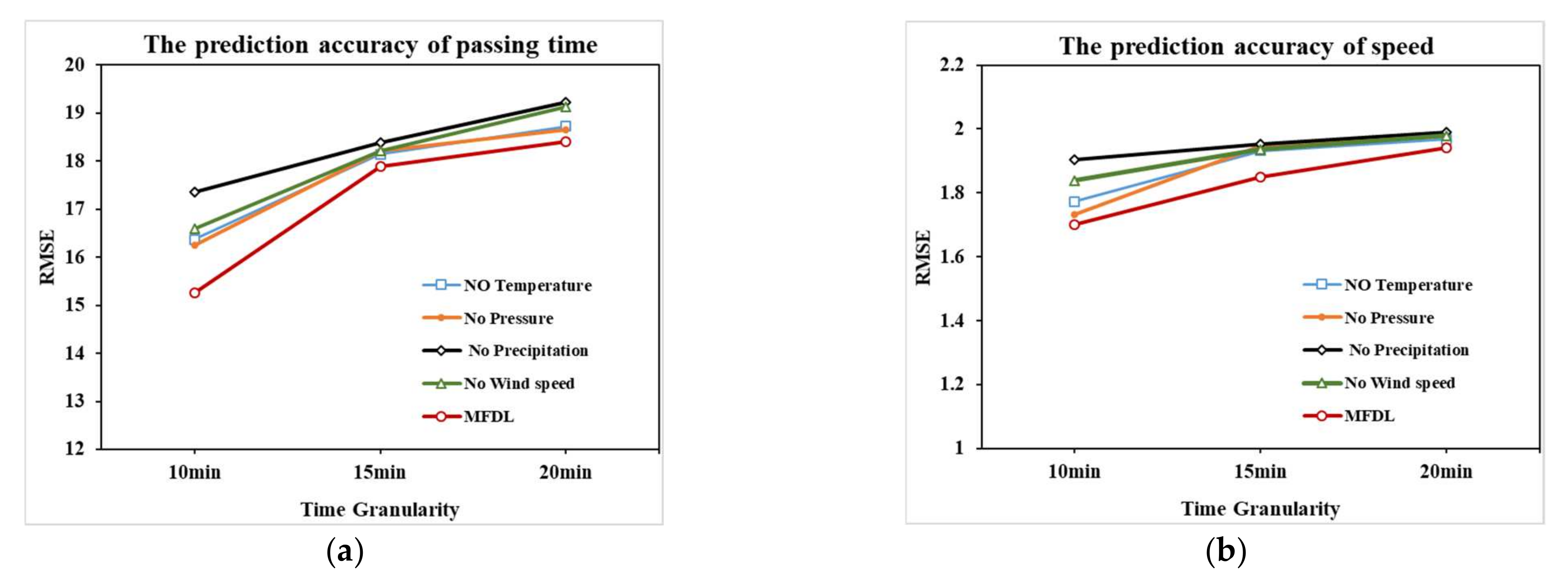
It has been explained that the weather has an impact on the prediction accuracy in Table 4. To further analyze the weather factors on prediction accuracy, we investigated and tested the model of weather effect, including four conditions: without temperature (i.e., No temperature model), without pressure (i.e., No pressure model), without precipitation (i.e., No precipitation model) and without wind speed (i.e., No wind speed model) (see Figure 19). It intuitively shows that the precipitation has a more significant impact on the prediction than other weather factors in different time granularity. It is not difficult to understand because the precipitation affects travel speed leading to the traffic operation state various, which verifies the previous research [43].
4. Discussion
In this study, we constructed a multi-task fusion deep learning framework for intersection traffic operation performance prediction. The passing time and the speed are selected to be prediction targets, which can reflect the process state and the visual state of the intersection operation performance.
In the data-collecting stage, the floating car data is used as the data source to verify the prediction model’s availability, which can reflect the traffic performance of large-scale intersection areas. The floating car data can accurately describe the upstream and downstream traffic state of the intersection, which makes up for the shortage of small coverage of fixed sensor data [16].
In the parameter extraction stage, we adopted the grid model, which can identify the intersections rapidly without the digital map. The novel grid model is proposed to extract the traffic parameters from the floating car data. On the one hand, the grid model simplifies the complex map-matching algorithm and improves the efficiency without the digital map. On the other hand, the intersection affected area and the direction of GFCD can be identified by the grid model and the fuzzy C-means (FCM) clustering method, which exceeded the limit of fixed influence area of intersection [44]. It indicated that the grid model has significant universality, which can be applied to other cities.
In the construction model stage, we design the MFDL framework of four variable groups. Meanwhile, to enhance the depth of the model, the ResNet is incorporated into the MFDL model, which can enhance the depth of the model and alleviate the problem of gradient disappearance [45]. The MFDL can capture the temporal, spatial, topology feature of the passing time and speed and the prediction results are promising. The two target predictions are negatively correlated, and the interplay between these two targeted prediction variables can significantly improve the prediction accuracy and efficiency, which is consistent with the studies of Kunpeng Zhang et al. [46]. This proposed method predicts the intersection operation performance in real-time and can provide valuable insights for traffic managers to improve the intersection’s operation efficiency.
There is more work ahead in the future development of this study. First, although accurate speed and time can be extracted from a single data source (i.e., FCD), it is difficult to estimate the actual traffic flow because the permeability cannot be obtained [47]. In order to comprehensively detect the operation performance of signalized intersections, it is necessary to import multi-source data, such as induction loop data [48], microwave data [49], etc., to extract traffic flow information. Second, in the passing time pattern, we consider the real-time and historical pattern. In future work, we will consider more passing time patterns to improve the accuracy. Lastly, the existing amount of data is enough to support the construction and validation of the model. Naturally, if a larger range of floating car data can be obtained in the future, using this proposed model to predict the traffic performance of intersections and validate the model will better reflect the universality of the model.
5. Conclusions
In this paper, a multi-task fusion deep learning framework is proposed for intersection traffic operation performance prediction. The passing time and the speed are selected to be prediction targets, which can reflect the intersection operation performance. The main conclusions of this paper are summarized as follows.
MFDL model enables us to capture the Spatio-temporal and topology feature of the traffic state efficiently. Comparisons with benchmark models show that the fusion deep learning model achieves the best prediction accuracy and robustness among the baseline model in different time granularity. In the process of STL and MFDL comparison, when the time granularity is 10 min and the epoch is 50, the training time is reduced by 8.3 min, and the efficiency increased by 46.42%, which means that the MFDL is more efficient. In the analysis of weather factors, the precipitation has a more significant impact on the prediction than other weather factors in different time granularities.
Future work will concentrate on exploring the novel deep learning structure based on the fusion method. For the influence factors of intersections operation state, we will consider multi-source input variables, including the time scheme, traffic flow, waiting time, etc., to improve the prediction accuracy.
Author Contributions
Conceptualization, D.C., X.Y.; methodology, D.C., X.Y.; software, D.C., S.L and L.W.; validation, D.C., X.Y., F.L., X.L., L.W. and S.L.; formal analysis, D.C, X.L.; investigation, D.C, X.L.; resources, D.C, X.Y.; data curation, D.C.; writing—original draft preparation, D.C., X.Y.; writing—review and editing, D.C., X.Y., F.L, X.L. and L.W.; visualization, D.C., S.L; supervision, X.Y.; project administration, D.C.; funding acquisition, X.Y. All authors have read and agreed to the published version of the manuscript.
Funding
This research was funded by National Key R&D Program of China (2019YFF0301403).
Data Availability Statement
The data presented in this study are available in DiDi. 2017. Available online: (http://www.xiaojukeji.com/en/company.html, accessed on 30 August 2017), Weather Data. Openly available online: (http://www.wheata.cn/, accessed on 30 August 2017).
Acknowledgments
Many thanks to the Institute of Policy Studies, DiDi Company for providing the data in this study.
Conflicts of Interest
The authors declare that there is no conflict of interest in any aspect of the data collection, analysis or the funding received regarding the publication of this paper.
References
- Khan, M.A.; Ectors, W.; Bellemans, T.; Janssens, D.; Wets, G. Unmanned Aerial Vehicle-Based Traffic Analysis: A Case Study for Shockwave Identification and Flow Parameters Estimation at Signalized Intersections. Remote Sens. 2018, 10. [Google Scholar] [CrossRef] [Green Version]
- Astarita, V.; Giofré, V.P.; Festa, D.C.; Guido, G.; Vitale, A. Floating Car Data Adaptive Traffic Signals: A Description of the First Real-Time Experiment with “Connected” Vehicles. Electronics 2020, 9, 114. [Google Scholar] [CrossRef] [Green Version]
- Yang, Y.; Yan, J.; Guo, J.; Kuang, Y.; Yin, M.; Wang, S.; Ma, C. Driving Behavior Analysis of City Buses Based on Real-Time GNSS Traces and Road Information. Sensors 2021, 21, 687. [Google Scholar] [CrossRef] [PubMed]
- Yu, J.; Stettler, M.E.J.; Angeloudis, P.; Hu, S.; Chen, X. (Michael). Urban Network-Wide Traffic Speed Estimation with Massive Ride-Sourcing GPS Traces. Transp. Res. Part C Emerg. Technol. 2020, 112, 136–152. [Google Scholar] [CrossRef]
- Garc, J.; Ramos, S. Impact of Inclement Weather on Traffic and Signal Timing Plan Optimization of Intersections in Nagaoka, Japan. Master’s Thesis, Universitat Politècnica de Catalunya, Barcelona, Spain, 2020. [Google Scholar]
- Dogramadzi, M.; Khan, A. Accelerated Map Matching for GPS Trajectories. IEEE Trans. Intell. Transp. Syst. 2021, 1–10. [Google Scholar] [CrossRef]
- Qiu, J.; Wang, R. Inferring Road Maps from Sparsely Sampled GPS Traces. J. Locat. Based Serv. 2014, 10, 111–124. [Google Scholar] [CrossRef]
- He, Z.; Zheng, L.; Chen, P.; Guan, W. Mapping to Cells: A Simple Method to Extract Traffic Dynamics from Probe Vehicle Data. Comput. Civ. Infrastruct. Eng. 2017, 32, 252–267. [Google Scholar] [CrossRef]
- Chen, D.; Yan, X.; Liu, F.; Liu, X.; Wang, L.; Zhang, J. Evaluating and Diagnosing Road Intersection Operation Performance Using Floating Car Data. Sensors 2019, 19, 2256. [Google Scholar] [CrossRef] [Green Version]
- Chen, C.; Hu, J.; Meng, Q.; Zhang, Y. Short-Time Traffic Flow Prediction with ARIMA-GARCH Model. In Proceedings of the 2011 IEEE Intelligent Vehicles Symposium (IV), Baden-Baden, Germany, 5–9 June 2011; pp. 607–612. [Google Scholar]
- Peksa, J. Prediction Framework with Kalman Filter Algorithm. Information 2020, 11, 358. [Google Scholar] [CrossRef]
- You, Z.; Chen, P. Efficient Regional Traffic Signal Control Scheme Based on a SVR Traffic State Forecasting Model BT—Internet of Vehicles—Safe and Intelligent Mobility; Hsu, C.-H., Xia, F., Liu, X., Wang, S., Eds.; Springer International Publishing: Cham, Switzerland, 2015; pp. 198–209. [Google Scholar]
- Sazi Murat, Y.; Baskan, Ö. Modeling Vehicle Delays at Signalized Junctions: Artificial Neural Networks Approach. J. Sci. Ind. Res. 2006, 65, 558–564. [Google Scholar]
- Hochreiter, S.; Schmidhuber, J. Long Short-Term Memory. Neural Comput. 1997, 9, 1735–1780. [Google Scholar] [CrossRef]
- Van Lint, H.; Van Hinsbergen, C. Short-Term Traffic and Travel Time Prediction Models. Transp. Res. Circ. 2012, 48–49. [Google Scholar]
- Chen, D.; Yan, X.; Liu, X.; Li, S.; Tian, X.; Wang, L.; Tian, X. A Multiscale-Grid-Based Stacked Bidirectional GRU Neural Network Model for Predicting Traffic Speeds of Urban Expressways. IEEE Access 2020, 9, 1321–1337. [Google Scholar] [CrossRef]
- Li, D.; Wu, J.; Xu, M.; Wang, Z.; Hu, K. Adaptive Traffic Signal Control Model on Intersections Based on Deep Reinforcement Learning. J. Adv. Transp. 2020, 2020, 6505893. [Google Scholar] [CrossRef]
- Zhao, L.; Song, Y.; Zhang, C.; Liu, Y.; Wang, P.; Lin, T.; Deng, M.; Li, H. T-GCN: A Temporal Graph Convolutional Network for Traffic Prediction. IEEE Trans. Intell. Transp. Syst. 2020, 21, 3848–3858. [Google Scholar] [CrossRef] [Green Version]
- Yu, B.; Yin, H.; Zhu, Z. Spatio-Temporal Graph Convolutional Networks: A Deep Learning Framework for Traffic Forecasting. In Proceedings of the Twenty-Seventh International Joint Conference on Artificial Intelligence, Stockholm, Sweden, 13–19 July 2018; pp. 3634–3640. [Google Scholar]
- Shi, X.; Chen, Z.; Wang, H.; Yeung, D.-Y.; Wong, W.; Woo, W. Convolutional LSTM Network: A Machine Learning Approach for Precipitation Nowcasting. In Proceedings of the 29th Annual Conference on Neural Information Processing Systems, NIPS 2015, Montreal, QC, Canada, 7–12 December 2015; Volume 28, pp. 802–810. [Google Scholar]
- Ke, J.; Zheng, H.; Yang, H.; Chen, X. (Michael). Short-Term Forecasting of Passenger Demand under on-Demand Ride Services: A Spatio-Temporal Deep Learning Approach. Transp. Res. Part. C Emerg. Technol. 2017, 85, 591–608. [Google Scholar] [CrossRef] [Green Version]
- Yu, B.; Lee, Y.; Sohn, K. Forecasting Road Traffic Speeds by Considering Area-Wide Spatio-Temporal Dependencies Based on a Graph Convolutional Neural Network (GCN). Transp. Res. Part C Emerg. Technol. 2020, 114, 189–204. [Google Scholar] [CrossRef]
- Zheng, C.; Fan, X.; Wang, C.; Qi, J. GMAN: A Graph Multi-Attention Network for Traffic Prediction. arXiv 2019, arXiv:10.1609/aaai.v34i01.5477. [Google Scholar]
- Liu, P.; Zhang, Y.; Kong, D.; Yin, B. Improved Spatio-Temporal Residual Networks for Bus Traffic Flow Prediction. Appl. Sci. 2019, 9, 615. [Google Scholar] [CrossRef] [Green Version]
- Zhang, J.; Zheng, Y.; Qi, D. Deep Spatio-Temporal Residual Networks for Citywide Crowd Flows Prediction. In Proceedings of the AAAI Conference on Artificial Intelligence 2017, San Francisco, CA, USA, 4–9 February 2017; Volume 31. [Google Scholar]
- Rezaei, S.; Liu, X. Multitask Learning for Network Traffic Classification. In Proceedings of the 2020 29th International Conference on Computer Communications and Networks (ICCCN), Honolulu, HI, USA, 3–6 August 2020; pp. 1–9. [Google Scholar]
- Jin, F.; Sun, S. Neural Network Multitask Learning for Traffic Flow Forecasting. In Proceedings of the 2008 IEEE International Joint Conference on Neural Networks (IEEE World Congress on Computational Intelligence), Hong Kong, China, 1–6 June 2008; pp. 1897–1901. [Google Scholar]
- Chen, Z.; Zhao, B.; Wang, Y.; Duan, Z.; Zhao, X. Multitask Learning and GCN-Based Taxi Demand Prediction for a Traffic Road Network. Sensors 2020, 20, 3776. [Google Scholar]
- Tian, X.; Chen, D.; Yan, X.; Wang, L.; Liu, X.; Liu, T. Estimation Method of Intersection Signal Cycle Based on Empirical Data. J. Transp. Eng. Part A Syst. 2021, 147, 04021001. [Google Scholar] [CrossRef]
- Liu, X.; Lu, F.; Zhang, H.; Qiu, P. Intersection Delay Estimation from Floating Car Data via Principal Curves: A Case Study on Beijing’s Road Network. Front. Earth Sci. 2013, 7, 206–216. [Google Scholar] [CrossRef]
- He, Z.; Qi, G.; Lu, L.; Chen, Y. Network-Wide Identification of Turn-Level Intersection Congestion Using Only Low-Frequency Probe Vehicle Data. Transp. Res. Part C Emergy Technol. 2019, 108, 320–339. [Google Scholar] [CrossRef]
- Dunn, J.C. A Fuzzy Relative of the ISODATA Process and Its Use in Detecting Compact Well-Separated Clusters. J. Cybern. 1973, 3, 32–57. [Google Scholar] [CrossRef]
- Cheng, Z.; Wang, W.; Lu, J.; Xing, X. Classifying the Traffic State of Urban Expressways: A Machine-Learning Approach. Transp. Res. Part A Policy Pract. 2020, 137, 411–428. [Google Scholar] [CrossRef]
- He, K.; Zhang, X.; Ren, S.; Sun, J. Deep Residual Learning for Image Recognition. Proc. IEEE Comput. Soc. Conf. Comput. Vis. Pattern Recognit. 2016, 2016, 770–778. [Google Scholar] [CrossRef] [Green Version]
- Zhang, J.; Chen, F.; Cui, Z.; Guo, Y.; Zhu, Y. Deep Learning Architecture for Short-Term Passenger Flow Forecasting in Urban Rail Transit. IEEE Trans. Intell. Transp. Syst. 2020, 1–11. [Google Scholar] [CrossRef]
- Li, Q.; Han, Z.; Wu, X.M. Deeper Insights into Graph Convolutional Networks for Semi-Supervised Learning. In Proceedings of the 32nd AAAI Conference Artificial Intelligence, New Orleans, LA, USA, 2–7 February 2018; pp. 3538–3545. [Google Scholar]
- Wheata. Available online: http://www.wheata.cn/ (accessed on 30 August 2017).
- Zhou, P.; Shi, W.; Tian, J.; Qi, Z.; Li, B.; Hao, H.; Xu, B. Attention-Based Bidirectional Long Short-Term Memory Networks for Relation Classification. In Proceedings of the 54th Annual Meeting of the Association for Computational Linguistics—Short Paperts, Berlin, Germany, 7–12 August 2016; pp. 207–212. [Google Scholar] [CrossRef] [Green Version]
- Abadi, M.; Agarwal, A.; Barham, P.; Brevdo, E.; Chen, Z.; Citro, C.; Corrado, G.S.; Davis, A.; Dean, J.; Devin, M. TensorFlow: Large-Scale Machine Learning on Heterogeneous Distributed Systems. arXiv 2015, arXiv:1603.04467. [Google Scholar]
- Ketkar, N. (Ed.) Introduction to Keras BT—Deep Learning with Python: A Hands-on Introduction; Apress: Berkeley, CA, USA, 2017; pp. 97–111. ISBN 978-1-4842-2766-4. [Google Scholar]
- Chandra, S.R.; Al-Deek., H. Cross-Correlation Analysis and Multivariate Prediction of Spatial Time Series of Freeway Traffic Speeds. Transp. Res. Rec. 2008, 2061, 64–76. [Google Scholar] [CrossRef]
- Chang, Y.; Wang, S.; Zhou, Y.; Wang, L.; Wang, F. A Novel Method of Evaluating Highway Traffic Prosperity Based on Nighttime Light Remote Sensing. Remote Sens. 2020, 12, 102. [Google Scholar] [CrossRef] [Green Version]
- Angel, M.L.; Sando, T.; Chimba, D.; Kwigizile, V. Effects of Rain on Traffic Operations on Florida Freeways. Transp. Res. Rec. 2014, 2440, 51–59. [Google Scholar] [CrossRef]
- Zhang, H.; Lu, F.; Zhou, L.; Duan, Y. Computing Turn Delay in City Road Network with GPS Collected Trajectories. In Proceedings of the 2011 International Workshop on Trajectory Data Mining and Analysis, Beijing, China, 17–21 September 2011; Association for Computing Machinery: New York, NY, USA, 2011; pp. 45–52. [Google Scholar]
- Zhang, K.; Liu, Z.; Zheng, L. Short-Term Prediction of Passenger Demand in Multi-Zone Level: Temporal Convolutional Neural Network with Multi-Task Learning. IEEE Trans. Intell. Transp. Syst. 2020, 21, 1480–1490. [Google Scholar] [CrossRef]
- Zhang, Z.; Li, M.; Lin, X.; Wang, Y. Network-Wide Traffic Flow Estimation with Insufficient Volume Detection and Crowdsourcing Data. Transp. Res. Part C Emergy Technol. 2020, 121, 102870. [Google Scholar] [CrossRef]
- Zhang, K.; Wu, L.; Zhu, Z.; Deng, J. A Multitask Learning Model for Traffic Flow and Speed Forecasting. IEEE Access 2020, 8, 80707–80715. [Google Scholar] [CrossRef]
- Kim, Y.; Wang, P.; Zhu, Y.; Mihaylova, L. A Capsule Network for Traffic Speed Prediction in Complex Road Networks. In Proceedings of the Sensor Data Fusion: Trends, Solutions, Applications, SDF 2018, Bonn, Germany, 9–11 October 2018. [Google Scholar] [CrossRef] [Green Version]
- Gu, Y.; Lu, W.; Qin, L.; Li, M.; Shao, Z. Short-Term Prediction of Lane-Level Traffic Speeds: A Fusion Deep Learning Model. Transp. Res. Part. C Emerg. Technol. 2019, 106, 1–16. [Google Scholar] [CrossRef]
Figure 1.
The flowchart of the prediction method.

Figure 2.
Diagram of intersection area; (a) trajectory points; (b) topology of intersection.

Figure 3.
Grid model.

Figure 4.
Identified the intersection area.

Figure 5.
Identified the direction of the trajectory.

Figure 6.
Residual block (a) Original structure; (b) Improved structure.

Figure 7.
Graph convolutional network.

Figure 8.
Multi-task fusion deep learning model framework.

Figure 9.
The passing time of the intersection.

Figure 10.
The order of FCD distribution (a) Hourly and (b) daily distributions of traffic flow at the selected intersections.
Figure 10.
The order of FCD distribution (a) Hourly and (b) daily distributions of traffic flow at the selected intersections.

Figure 11.
The average speed and the passing time on weekdays and weekends; (a) The speed (b) The passing time.
Figure 11.
The average speed and the passing time on weekdays and weekends; (a) The speed (b) The passing time.

Figure 12.
The correlation degree of intersection.

Figure 13.
The training epoch: (a) the total training process; (b) the passing time and speed training process separately.
Figure 13.
The training epoch: (a) the total training process; (b) the passing time and speed training process separately.

Figure 14.
Comparison of the prediction errors for each method. (a) MAE of the predicted passing time; (b) MAE of the predicted speed; (c) RMSE of the predicted passing time; (d) RMSE of the predicted speed.
Figure 14.
Comparison of the prediction errors for each method. (a) MAE of the predicted passing time; (b) MAE of the predicted speed; (c) RMSE of the predicted passing time; (d) RMSE of the predicted speed.

Figure 15.
Comparison of different methods in terms of various time steps. (a) the speed (b) the passing time.
Figure 15.
Comparison of different methods in terms of various time steps. (a) the speed (b) the passing time.

Figure 16.
The absolute errors and the relative errors of MFDL: (a) the absolute errors of the passing time; (b) the relative errors of the passing time; (c) the absolute errors of speed; (d) the relative errors of speed.
Figure 16.
The absolute errors and the relative errors of MFDL: (a) the absolute errors of the passing time; (b) the relative errors of the passing time; (c) the absolute errors of speed; (d) the relative errors of speed.

Figure 17.
The prediction accuracy in different time of day: (a) The prediction accuracy of the passing time; (b) The prediction accuracy of speed.
Figure 17.
The prediction accuracy in different time of day: (a) The prediction accuracy of the passing time; (b) The prediction accuracy of speed.

Figure 18.
Prediction precision of the passing time and speed in different directions. (a) the prediction precision of the passing time; (b) the prediction precision of speed.
Figure 18.
Prediction precision of the passing time and speed in different directions. (a) the prediction precision of the passing time; (b) the prediction precision of speed.

Figure 19.
Influence of weather factors on prediction accuracy: (a) the prediction accuracy of the passing time; (b) the prediction accuracy of speed.
Figure 19.
Influence of weather factors on prediction accuracy: (a) the prediction accuracy of the passing time; (b) the prediction accuracy of speed.


Table 1.
The detailed data attributes of the FCD system.
| Characteristic | Field Name | Field Type | Field Description |
|---|---|---|---|
| Order ID | String | Marking each vehicle | |
| Timestamp | Timestamp | Accurate to second | |
| Longitude | Floating | Accurate to six decimal places | |
| Latitude | Floating | Accurate to six decimal places | |
| v | Vehicle Speed | Integer | Kilometer per hour |
Table 2.
Examples of weather-condition data.
| Date/Time | Temperature | Pressure | Precipitation | Wind Speed |
|---|---|---|---|---|
| 1 August 2017 6:00 | 37.9 | 979.8 | 0.0005 | 4.20 |
| 1 August 2017 7:00 | 37.3 | 979.3 | 0.0005 | 4.56 |
| 1 August 2017 8:00 | 36.2 | 979.1 | 0.0004 | 4.78 |
| 1 August 2017 9:00 | 33.6 | 979.2 | 0.0003 | 4.83 |
Table 3.
Hyper-parameter setting.
| Variable | Passing Time | Speed | Graph | Weather |
|---|---|---|---|---|
| Number of filters | 32 and 64 | 32 and 64 | 32 and 64 | - |
| Kernel size | - | |||
| FC layers | 92 | 92 | 92 | 92 |
| Hidden units | - | - | - | 128 |
Table 4.
Compare the prediction performance with different models.
| Target | Tg | Category | MS | ML | DL | MFDL | ||||||
|---|---|---|---|---|---|---|---|---|---|---|---|---|
| Indicators | ARIMA | SVR | LSTM | GRU | CNN | Conv-LSTM | No-CNN | No Graph | NoWeather | MFDL | ||
| Speed | 10 | RMSE | 3.64 | 2.43 | 2.29 | 1.98 | 1.99 | 1.97 | 1.96 | 1.92 | 1.90 | 1.70 |
| MAE | 2.63 | 2.01 | 1.62 | 1.71 | 1.58 | 1.51 | 1.82 | 1.42 | 1.36 | 1.29 | ||
| WMAPE | 30.29% | 24.54% | 19.88% | 20.90% | 18.98% | 18.03% | 22.34% | 17.31% | 16.65% | 15.82% | ||
| 15 | RMSE | 3.99 | 2.69 | 2.19 | 2.06 | 1.98 | 2.31 | 2.00 | 1.98 | 1.96 | 1.85 | |
| MAE | 2.93 | 2.87 | 1.62 | 1.52 | 1.52 | 1.60 | 1.52 | 1.46 | 1.44 | 1.42 | ||
| WMAPE | 32.91% | 25.48% | 20.32% | 21.32% | 20.54% | 20.10% | 19.06% | 18.28% | 18.11% | 15.95% | ||
| 20 | RMSE | 4.39 | 3.44 | 2.06 | 2.19 | 3.31 | 3.06 | 2.18 | 2.01 | 1.98 | 1.94 | |
| MAE | 3.05 | 2.92 | 1.53 | 1.51 | 2.61 | 2.17 | 1.56 | 1.44 | 1.45 | 1.43 | ||
| WMAPE | 37.35% | 26.43% | 24.50% | 24.69% | 23.17% | 23.61% | 19.64% | 18.82% | 18.47% | 17.97% | ||
| Passing time | 10 | RMSE | 30.27 | 25.73 | 19.72 | 19.87 | 18.24 | 17.25 | 18.64 | 18.23 | 16.19 | 15.26 |
| MAE | 24.90 | 23.92 | 13.87 | 13.93 | 13.43 | 12.34 | 13.41 | 13.39 | 11.24 | 10.86 | ||
| WMAPE | 43.39% | 39.05% | 25.31% | 22.42% | 22.04% | 22.69% | 22.34% | 22.23% | 20.52% | 19.76% | ||
| 15 | RMSE | 31.39 | 26.06 | 22.28 | 19.95 | 18.78 | 19.16 | 20.12 | 19.66 | 19.07 | 17.89 | |
| MAE | 25.25 | 24.17 | 15.65 | 14.28 | 14.92 | 12.67 | 14.30 | 13.65 | 13.33 | 12.59 | ||
| WMAPE | 46.27% | 44.14% | 24.86% | 24.52% | 23.12% | 23.14% | 26.12% | 24.93% | 24.34% | 22.99% | ||
| 20 | RMSE | 32.77 | 28.23 | 22.78 | 20.78 | 19.36 | 20.12 | 20.52 | 20.67 | 21.04 | 18.41 | |
| MAE | 27.78 | 26.39 | 16.06 | 14.65 | 15.24 | 13.37 | 14.42 | 13.82 | 14.14 | 13.16 | ||
| WMAPE | 49.93% | 47.97% | 25.51% | 25.28% | 25.26% | 24.31 | 26.18% | 25.12% | 24.70% | 23.94% | ||
Table 5.
The comparison of signal-task prediction and multi-task prediction.
| Tg | Metrics | Passing Time of STL | Speed of STL | Passing Time of MFDL | Speed of MFDL |
|---|---|---|---|---|---|
| 10 min | RMSE | 16.39 | 1.90 | 15.26 | 1.7 |
| MAE | 11.42 | 1.37 | 10.86 | 1.29 | |
| WMAPE | 20.84% | 16.74% | 19.76% | 15.82% | |
| Training time | 13.4 + 13.4 = 26.8 min | 18.3 min | |||
| 15 min | RMSE | 17.92 | 1.94 | 17.89 | 1.85 |
| MAE | 12.79 | 1.48 | 12.59 | 1.42 | |
| WMAPE | 23.36% | 17.07% | 22.99% | 15.95% | |
| Training time | 9.2 + 9.2 =18.4 min | 12.5 min | |||
| 20 min | RMSE | 19.14 | 2.14 | 18.41 | 1.94 |
| MAE | 13.71 | 1.56 | 13.16 | 1.43 | |
| WMAPE | 24.93% | 19.80% | 23.94% | 17.97% | |
| Training time | 6.7 + 6.7 = 13.4 min | 9.25 min | |||
Publisher’s Note: MDPI stays neutral with regard to jurisdictional claims in published maps and institutional affiliations. |
© 2021 by the authors. Licensee MDPI, Basel, Switzerland. This article is an open access article distributed under the terms and conditions of the Creative Commons Attribution (CC BY) license (https://creativecommons.org/licenses/by/4.0/).
Share and Cite
MDPI and ACS Style
Chen, D.; Yan, X.; Liu, X.; Wang, L.; Li, F.; Li, S. Multi-Task Fusion Deep Learning Model for Short-Term Intersection Operation Performance Forecasting. Remote Sens. 2021, 13, 1919. https://0-doi-org.brum.beds.ac.uk/10.3390/rs13101919
AMA Style
Chen D, Yan X, Liu X, Wang L, Li F, Li S. Multi-Task Fusion Deep Learning Model for Short-Term Intersection Operation Performance Forecasting. Remote Sensing. 2021; 13(10):1919. https://0-doi-org.brum.beds.ac.uk/10.3390/rs13101919
Chicago/Turabian StyleChen, Deqi, Xuedong Yan, Xiaobing Liu, Liwei Wang, Fengxiao Li, and Shurong Li. 2021. "Multi-Task Fusion Deep Learning Model for Short-Term Intersection Operation Performance Forecasting" Remote Sensing 13, no. 10: 1919. https://0-doi-org.brum.beds.ac.uk/10.3390/rs13101919
Note that from the first issue of 2016, this journal uses article numbers instead of page numbers. See further details here.