Using High-Spatial Resolution UAV-Derived Data to Evaluate Vegetation and Geomorphological Changes on a Dune Field Involved in a Restoration Endeavour

Abstract

Nowadays, the employment of high-resolution Digital Surface Models (DSMs) and RGB orthophotos has become fundamental in coastal system studies. This work aims to explore the potentiality of low-cost Unmanned Aerial Vehicle (UAV) surveys to monitor the geomorphic and vegetation state of coastal sand dunes by means of high-resolution (2–4 cm) RGB orthophotos and DSMs. The area of study (Punta Marina, Ravenna, Italy), in the North Adriatic Sea, was considered very suitable for these purposes because it involves a residual coastal dune system, damaged by decades of erosion, fragmentation and human intervention. Recently, part of the dune system has been involved in a restoration project aimed at limiting its deterioration. RGB orthophotos have been used to calculate the spectral information of vegetation and bare sand and therefore, to monitor changes in their relative cover area extension over time, through the using of semi-automatic classification algorithms in a GIS environment. Elevation data from high-resolution DSMs were used to identify the principal morphological features: (i) Dune Foot Line (DFL); (ii) Dune Crest Line (DCL); Dune seaward Crest Line (DsCL); Stable Vegetation line (SVL). The USGS tool DSAS was used to monitor dune dynamics, considering every source of error: a stable pattern was observed for the two crest lines (DCL and DsCL), and an advancing one for the others two features (DFL and SVL). Geomorphological data, as well as RGB data, confirmed the effectiveness of planting operations, since a constant and progressive increase of the vegetated cover area and consolidation of the dune system was observed, in a period with no energetic storms. The proposed methodology is rapid, low-cost and easily replicable by coastal managers to quantify the effectiveness of restoration projects.

1. Introduction

Coastal sand dunes represent an important resource for coastal areas, not only because they represent a crucial sediment supply for the dune-beach system [1], but also because they act as a first line of coastal defence against sea intrusion, attenuating the impact of storms and storm surges and preventing salt water leakage into the aquifer [2,3]. They also represent a unique habitat for specialised species, both animal and vegetal, constituting an irreplaceable ecosystem. For all these reasons, coastal managers must prioritise the preservation of coastal sand, given their environmental and economic value.

According to many authors, coastal sand dunes are aeolian morphological elements modelled by the dynamic of several forcing factors, mainly marine and aeolian forces and the vegetation conditions [4,5,6,7,8,9]. On the one hand, the sea action determines beach morphological characteristics and provides sand supply to nourish the dune [10,11], but, on the other hand, it can also be a strong cause of erosion when storms occur. The connection between dune morphology and sea action is very strong, as dunes are the “foremost elements at the edge of the backshore, reflecting the short-, medium- and long-term surfzone-beach-dune processes operating on any particular beach” [12,13,14]. The wind, especially blowing onshore, represents the builder force that transports sand from the beach to the dune, where the decrease of energy and the presence of specialised vegetation trapping the sand, increase dune mass: this implicates that the aeolian climate (direction, frequency, speeds, etc.) of a region is one of the most influencing factors in dune morphology and evolution. Like the sea action, wind can also have an erosive effect; it can remove the sand by blowing on a specific part of the dune field where the vegetation is deteriorating or has been removed or excavated within the dune body. This process represents a major damaging factor because it tends to feed itself: as the wind digs into the dune, blowing into an increasingly narrower space, it accelerates and intensifies its erosion potential [15]. According to Hesp [16], this dynamic creates “blowouts”, (saucer-, cup- or through-shaped) depressions or hollows with a derived depositional lobe formed by wind erosion [17,18]. Just like the previous two forcing factors, vegetation has a multi-level influence on the dune’s morphology, since geomorphology and vegetation dynamics are naturally interrelated and affect each other considerably [19]. Always acting as a stabilising factor right from the early stages of dune life, vegetation can positively affect soil consolidation and can slow down the wind’s speed, thereby reducing its sediment transport capability. The process usually follows well-defined steps: a very specialised vegetation colonises the dune habitat, which is characterised by extreme conditions regarding several environmental parameters (i.e., temperature, sand soil, salty air spray, salty water). The vegetation is usually organised by phyto-sociological successions, starting from pioneer species which allow the germination of many other vegetal forms (annual, perennial, grasses, bushes, trees), thus modifying the soil and consolidating it by means of roots and gradually enriching it with nutrients. The vegetation complex effect on morphology can depend on several secondary factors, such as plant species, growing rate, density, distribution or plant height [20]. According to Hesp [6], plant density is probably the most influencing factor because of its effect on wind speed and sand deposition. A high plant density decreases the degree of near-surface flow penetration, while drag increases [5].

Apart from all these natural factors, human activities are an important component, especially in the last century, which is characterised by an increased human pressure on the coast; erosion, fragmentation, dismantlement, as well as interference in the biosphere, are only some of the human-induced perturbations. In recent years, coastal managers have tried to attenuate the influence of human pressure, conceiving and applying different restoration techniques aiming to reactivate original morphological and ecological integrity [21]. These techniques principally employ two kind of approaches that are always integrated [22]: (i) construction of “hard” structures, such as semipermeable wooden fences [23,24,25], conceived to improve the deposition of wind-blown sand, to reduce tourist trampling and to protect the original dune species; (ii) re-vegetation efforts that have become very popular in recent years, due to the pivotal role that vegetation plays in this environment. Re-vegetation favours the consolidation of dune’s loose sediments thanks to the roots’ action; it dissipates storm wave energy and improves the capability of trapping the sand transported by wind, thus constantly incrementing dune growth. All these efforts have been recently defined as “dune gardening”, a term referring to modern coastal management which aims to maximise biodiversity and preserve priority species, resulting in a preservation of the dune status which mainly follows human wish lists rather than natural evolution, with little knowledge on dunes’ life stages in a wider and millennial context [26]. Despite the lack of a wider and long-term vision, especially in the Mediterranean context where dunes and coastal environments have always been subordinated to human will [27], recent remote sensing techniques can help to understand in detail the physical influence and the effectiveness of such restoration projects on dune environments.

Recent studies focused on the dynamic interaction between the beach and the dune system when restoration projects are in place [28,29], but due to the lack of high-resolution and large-scale morphological data across the entire beach-dune system, this interaction is still poorly understood [30]. Furthermore, the sustainability and efficiency of such nature-based solutions requires a multidisciplinary approach combined with a long-term monitoring and a quantification of the dune dynamism with high-resolution data [29]. With regards especially to vegetation replanting intervention, according to Sigren [31], there is a lack of quantitative studies and a scarce knowledge of the impact of plants on protecting the dune from erosion.

In recent decades, the development of many high-accuracy remote sensing (RS) techniques has introduced several advantages: they now allow the acquisition of much more accurate data, with a much higher survey frequency. This can be fundamental to dune systems study, because it allows researcher to perform multi-scale analyses, that are crucial to understanding the complex connection between dynamic factors influencing dune fields [32]. Among RS techniques, the most appropriate for usage in dune environment are: (i) Laser Scanning (LS), airborne or terrestrial, especially for high-resolution monitoring of linear-shaped morphologies [33,34]; (ii) Structure from Motion (SfM) photogrammetry, usually from Unmanned Aerial Vehicles (UAV) [35,36,37,38,39,40]. Sediment distribution related to vegetation types on coastal dunes can be investigated combining airborne multispectral and LiDAR dataset [41], but low cost UAVs have several advantages, being usually light-weight devices, that are easily transported and very fast performing. This increases the surveys’ frequency and allows conditions for building high resolution orthomosaics, as well as point clouds and digital surface models with a resolution of few centimetres. Further advancements in the analysis of satellite images (i.e., Sentinel-2 programme) can now be applied for low resolution phenology studies of coastal dunes [42], whereas huge potential is given by UAVs when combined with multispectral data for plant species discrimination at high resolution [36,43]. Attempts to distinguish among dune vegetation communities using UAV equipped with multispectral cameras (red, green and near-infrareds bands) have been performed by [44] and allowed to produce vegetation maps at 0.15 m resolution by means of pixel-oriented and object-oriented algorithms.

For this study, a UAV monitoring program was conceived in order to survey the influence of a restoration project, undertaken by the local municipality, on the spatial vegetation cover and the geomorphic evolution of a residual coastal dune field. The restoration project aimed to stop the dune erosional trend and to reactivate the natural dynamics of the dune system by improving its natural resilience in a local context of strong and long-lasting human intervention and destabilisation of the coastal environment. The project included wooden fences and raised footpaths, and replantation of endemic species in the foredune in order to reduce the erosion that is mainly due to trampling by beach users on the seaward side of the dune. The aim of the paper is to test if low cost and high-resolution drone-derived products (RGB orthophotos and Digital Surface Models), combined with semi-automatic Geographic Information System (GIS) tools, are suitable and rapid methods to identify and quantify the spatial vegetation cover variation and the geomorphic evolution of the dune through time. The low-cost survey techniques and rapid GIS analyses used in this paper are believed to be replicable by local managers to easily track the overall effectiveness of restoration projects when expensive multispectral cameras or LiDAR data are not available.

2. Study Area

The area of study is located in Punta Marina, a renowned Italian seaside town along the North Adriatic Sea coast, within the Ravenna municipality. The dune field is a residual of a much more continuous dune ridge, which human activities connected to tourism have largely damaged and fragmented during the last 50 years by [45,46]. The Ravenna coastal belt is about 50 km long and is dominated by intermediate to dissipative, mild-slope beaches [47]; the majority of these beaches are oriented NNW-SSE, according to the dominant currents and wind direction, and the beaches show an erosive trend, that is connected not only to human activities and land use, but also to strong alongshore drift, typically from South to North in this part of Adriatic sea [48,49].

In spring/summer, the aeolian climate is dominated (in terms of energy) by SE and NE wind [50] (“Scirocco” and “Bora”, respectively), while in the autumn/winter season winds blow more frequently from W-WNW [51]. Marine condition are dominated by SE and NE currents, with a low-energy wave climate [52], while the tidal regime is semidiurnal and diurnal having comparable amplitude [53,54], from 0.3–0.4 m (neap tide) to 0.8–0.9 m (spring tide).

The investigated dune field is located along a 500 m section of the urbanised Ravenna coast, which is the only area where building is forbidden by law and economic exploitation of the beach is off-limits in an area also known as “public beaches”. In this segment of the coast, beaches are largely protected by breakwaters and groins. The beach has an average width of about 70–80 m, and periodically it receives nourishments to counteract beach erosion [55].

From a morphological point of view, the dune ridge is constituted by two segments (a northern and a southern one), separated by a large access pathway to the beach. The whole dune is constrained on both lateral sides by walkways and, on the backside, by a dense pinewood, grown above the paleo-dune ridges. The natural morphology of this dune is also influenced on the seaward side by sand mounds (“winter dunes” or “artificial dunes”) artificially built by beach scraping and sand nourishment, accumulating sand taken from adjacent zones [56,57], with the aim of protecting touristic structures (beach huts, also locally called “bagni”) during the winter season. The dune presents a “barchanoidal” shape, influenced by the artificial dune accumulation that is carried out every winter [58]. Despite all these artificial constrictions, the dune ridge preserves its natural dynamics, exceeding in some parts an elevation of 5.80 m above m.s.l.

With regard to vegetation, the typical zonation of the north Adriatic coastal dunes, sea to land sequence, firstly consists of annual pioneer species, Salsola kali–Cakiletum maritimae (EUNIS Code B1.12), growing closest to the shoreline. Then Agropyretum, Echinophoro spinosae–Elymetum farcti (EUNIS Code B1.3), which includes the so-called psammophilous vegetation, from coastal sandy and fine-pebbly dunes throughout the Mediterranean region [59], as well as the Echinophoro spinosae–Ammophiletum australis (EUNIS Code B1.3) class; together these two classes usually occupy the largest part of the dune surface and represent the semi-stable vegetation of the dune. Moving landward, according to Pignatti (1952), the grey dune vegetation is made by “perennial dry short-grasslands, whose structure is mainly determined by a thick carpet of cryptogams, among which there are therophytes, hemicryptophytes and chamaephytes”, namely the Tortulo–Scabiosetum class (EUNIS Code B1.4); the Juniperus communis and the Hippophaetum fluviatilis association (EUNIS Code B1.63), which represents the bush strip on the stable dune. Lastly, a coastal pine woods (EUNIS Code B1.7) closes the sequence [60].

In May 2015, local authorities conceived a plan for the dune restoration to reduce the increasing erosion and contain the geomorphic and vegetation deterioration. In 2015, before the implementation of dune restoration actions, the erosion was mainly due to trampling by beach users as accelerated by wind action, and it occurred primarily on the seaward side of the dune, as well as in several blowouts located in the northern section. To improve sand trapping [61,62,63], the restoration project included a 1-m elevated wooden pathway crossing the dune system and a wooden fence, built in front of the dune foot. In 2016, 5500 native dune plants were planted to accelerate growth of the incipient dune and strengthen stability of the whole system. 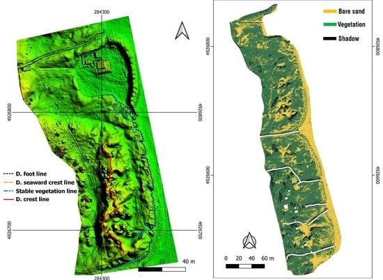The principal species chosen were Agropyron junceum and Ammophila arenaria, renowned to have a strong effect on the wind flow thanks to its high and dense canopies [64] and Euphorbia paralias, that is the species with the highest capability in sand trapping and dune stabilization [49]. The surveys were limited to the zone within the red line in Figure 1, with an extension of about 31,568 m². This specific area of interest was chosen in order to delimit the morphological analysis exclusively to the dune’s domain area, to exclude the pinewood, which would have strongly influenced both classification and morphological analysis.

3. Materials and Methods

3.1. Field Surveys

Topographic surveys were performed with a commercial DJI Phantom 3 Professional quadcopter, equipped with a standard digital camera of 12 megapixels and assisted by a high accurate differential GNSS equipped with Real Time Kinematic (RTK) technology for corrections (Trimble R6). Four surveys were carried out: two in 2017, on the 3rd of July and 13th of December, one in April 2018 and the last in February 2020. All flights were planned with a freeware application and performed in automatic mode, in order to guarantee the survey’s high quality [65,66,67]. Flight general parameters are summarised in

Table 1. Principal parameters of the four UAV survey flights.

Survey	Nr. Images	Coverage Area (km)	Image Overlap (%)	Flight Speed (km/h)
3 March 2017	297	0.218	72	10
13 December 2017	150	0.129	72	10
18 April 2018	150	0.168	72	10
19 February 2020	130	0.142	72	10

.

Twenty ground control points (GCPs) were distributed on the beach and all over the dune field (Figure 2); the differential GNSS was used to measure each GCP centre position with millimetric precision, which is crucial to the photogrammetric reconstruction process.

The licensed software Agisoft Metashape Professional 1.5.1 [68] was used to reconstruct the digital model of the surveyed environment, thanks to the Structure from Motion (SfM) algorithm [69]; there followed the definition of Digital Surface Models (DSM) and very highly accurate ortho-photographs, composed by a mosaic of single orthogonal frames (orthomosaics).

Both DSMs and orthophotographs/mosaics were shaped with a resolution of 0.05 m and referenced to a global coordinate UTM system (ETRF 2000). For each survey, a validation of the DSM against RTK-DGNSS elevations measured along four profiles was performed (Figure 1). The validation profiles were traced from the end of the pinewood to the beach, taking care of measuring points in each morphological zone of the system (i.e., the stable paleo-dune, the backward dune depression, the foredune crest and foot and the emerged beach). For each survey, the Root Mean Square Error (RMSE) of elevation data was calculated (

Table 2. RMSE of elevation data for each survey resulting from the validation process.

Survey	RMSE
3 March 2017	0.08
13 December 2017	0.07
18 April 2018	0.06
19 February 2020	0.05

).

3.2. Post Processing and Analysis

3.2.1. RGB Data Analysis

Data from orthomosaics were analysed in GIS environment using freeware Qgis, version 3.12 and the plug-in for multispectral (satellite) images analysis Semi-automatic Classification Plug-in [70], named SCP. This plug-in, developed to analyse data from satellite multispectral images, offers very useful tools to work with RGB images.

UAV’s digital RGB images has 4 channels: 3 for visible bands, Red (λ = 625–740 nm), Green (λ = 520–565 nm), Blue (λ =500–520 nm) and a 4th, called alpha channel that controls the transparency/opacity of pixels. Before being processed for a pixel-based classification, images have firstly to be re-elaborated, creating separate channels for each orthomosaic and re-aggregating RGB data only, to obtain 3-bands images (SCP pre-processing tools). Indeed, pixel-based classification uses only spectral information to classify homogeneous groups of pixels, and it is widely used especially for land cover mapping purposes [71,72,73].

The second step was the creation of spectral information files (Figure 3), a so-called “Training Input”, whose algorithm “learns” to classify the relative image portions. In this study, the process consisted of drawing polygons corresponding to three different macro-classes: bare sand, vegetation and shadow. For each macro-class, a different number of categories was chosen to compose the training input file: for “bare sand”, polygon samples were drawn on the beach, blowouts and paths; “vegetation” was classified via collections of pioneer vegetation, ammophyle vegetation, grasses, bushes and trees samples. As for the “shadow” macroclass, its quantification depended on the environmental condition at the time of the survey (i.e., the season, the relative position of the sun, the weather and cloud conditions).

Because of very different states of illumination and shadow, due to the season, the time of the day and environmental conditions during surveys, a specific training input must be calibrated for each orthomosaic image.

Once the training input was calibrated, the choice of the most proper algorithm to be applied to the land cover spectral information classification prepared the initial semi-automatic classification. In this work, three algorithms have been tested: Maximum Likelihood (ML), Minimum Distance (MD), Spectral Distance (SD). The ML algorithm calculated the probability distributions for the macro-classes, estimating if a pixel belonged to one land cover class or another, so that the training input requires a large number of pixels for the spectral information calculation [74]. The Minimum Distance algorithm calculated the Euclidean distance between spectral information of image pixels and training spectral information, attributing pixels to different classes, based on the distance [70]. The SD algorithm calculates the spectral angle between spectral information of image pixels and training spectral information [75].

The classification process was limited to the AOI to avoid including the pinewood and the beach, thereby simplifying calculations and preventing data overload. Artificial structures, such as promenades or buildings, were manually removed from the orthomosaic, to facilitate the calculations. Shadows were treated as “no-data”, so for each algorithm calculation, shadows areas of all surveys were summed, building an overall mask, that was used to hide the correspondent parts in each classification raster map, thus analysing only data without shadows. Quantitative data, such as land cover area extension for each macro-class, could then be extrapolated from the classified image.

3.2.2. Morphological Analysis and Error Calculation

With the aim of analysing how the dune system responded, from a morphological point of view, to the restoration intervention, the following morphological elements were identified and mapped: dune foot line, dune crest line, dune seaward crest line and stable vegetation line.

• The Dune Foot Line (DFL) represents the most seaward limit of the dune and morphologically it is identified as an abrupt change in slope over a relatively short distance [76]. According to several authors [77,78], calculating DSM surface slopes and overlapping elevation contour lines to the DSM, is a reliable method to understand where the abrupt change of slope is located, in order to properly identify the dune foot line (Figure 4).
• The Dune Crest Line (DCL) is identified by “the highest-elevation peak landward of the shoreline and within a user-defined beach width” [79], thus dune crest position can be identified as the highest elevation point closest to the shoreline (Figure 5): 0.1 m overlapped contours to the elevation model proved to be very well suited to accomplish this task.
• The Dune seaward Crest Line (DsCL) refers to the morphology of the northern part of the system where in the last 10 years beach management has modified the dune morphology and an incipient foredune has formed in the seaward part of the dune system. Due to the DsCL morphology, the same methodology used to identify the DCL can be applied (Figure 5).
• The Stable Vegetation line (SVL) is basically determined by the borders of Agropyretum and Ammophyletum. At these latitudes the two communities often merge [44] being both perennial herbaceous vegetation typical of embryonal and white dunes of the Mediterranean [80]. This line was traced from the high spatial resolution (0.05 m) orthomosaics (Figure 6).

Once morphological elements were identified, the freeware tool for GIS Digital Shoreline Analysis System (DSAS) 4.3 version [81] was applied to monitor the variation trend of these linear elements and quantify their movements through time. This tool, implemented to estimate shoreline temporal changes, allows calculation of both absolute distances for almost any linear morphological feature and rates between consecutive surveys.

From the different indexes calculated by the tool, the following were chosen to be computed on 2 m spaced transects:

• Net Shoreline Movement (NSM): distance between the oldest and the most recent linear element, for each transect.
• End Point Rate (EPR): rate calculated considering the distance covered by each feature in relation to the time interval between the oldest and the most recent one.
• Confidence of End Point Rate (ECI or EPRunc in newer versions of DSAS): this index takes into consideration the uncertainty of lines (accuracy error) as a factor for calculating the EPR confidence.

It should be noted that, since each linear feature resulted to have a different length, the total number of transects varied in each case: 184 for the SVL, 167 for the DFL, 152 for the DCL and 57 for the DsCL.

In order to calculate the uncertainty of each line, several sources were considered:

• Pixel error: the spatial resolution of the digital model or image;
• GCP error (Figure 2): calculated by Photoscan software, during the model reconstruction process;
• GPS error: estimated as a maximum of 0.05 m, applying RTK technology;
• Digitizing error: calculated by delineating the same feature several times (in this case four) on the same orthomosaic and calculating the Root Mean Square Error of position residuals at regular intervals for that feature [67,68,69]. The position residuals between each pair of morphological lines were calculated by the “spatial adjustment” tool of Arcmap 10.1 (ESRI).

  Table 3. Digitising error in m for each couple of lines tested. Roman numerals indicate the identification number of the digitisation test.

  	Dune Foot Line				Dune Crest Line
  	Mar-17 I	Dec-17 II	Apr-18 III	Feb-20 IV	Mar-17 I	Dec-17 II	Apr-18 III	Feb-20 IV
  I–II	0.29	0.21	0.32	0.46	0.18	0.19	0.20	0.16
  I–III	0.28	0.30	0.38	0.31	0.16	0.23	0.16	0.13
  I–IV	0.34	0.26	0.37	0.29	0.24	0.17	0.18	0.19
  	Dune Seaward Crest Line				Stable Vegetation Line
  	Mar-17 I	Dec-17 II	Apr-18 III	Feb-20 IV	Mar-17 I	Dec-17 II	Apr-18 III	Feb-20 IV
  I–II	0.33	0.35	0.30	0.36	0.73	0.73	0.76	0.68
  I–III	0.26	0.37	0.31	0.31	0.82	0.56	0.54	0.62
  I–IV	0.31	0.38	0.29	0.35	0.84	0.79	0.65	0.57

  reports RMSE values calculated for each morphological feature; for each comparison, the highest value was taken as the uncertainty value.

4. Results

4.1. Semi-Automatic Classification Results

SCP results are summarised in

Table 4. Semi-automatic classification results in terms of m² and percentage. The results from all the three algorithms are reported.

Survey/Date	Algor.	Bare Sand		Vegetation		No Data
		m2	%	m2	%	%
1. March 2017	ML	11,928.2	41.0	17,123.6	58.9	0.1
	MD	13,305.1	49.5	13,536.2	50.4	0.1
	SD	14,609.3	54.4	12,211.1	45.5	0.1
2. December 2017	ML	10,354.2	35.6	18,697.9	64.3	0.1
	MD	10,822.8	40.2	16,044.1	59.7	0.1
	SD	6791.0	25.3	20,029.5	74.6	0.1
3. April 2018	ML	7552.1	25.9	21,499.2	74.0	0.1
	MD	8489.5	31.6	18,377.8	68.3	0.1
	SD	11,553.2	43.0	15,267.2	56.9	0.1
4. February 2020	ML	7605.0	26.1	21,446.8	73.8	0.1
	MD	9572.6	35.6	17,294.6	64.3	0.1
	SD	5428.5	20.2	21,391.5	79.7	0.1

for the three algorithms; although all three algorithms were able to identify the three macro-classes (bare sand, vegetation and shadow), only values calculated by the “Maximum Likelihood” algorithm were considered reliable. Since the same AOI was considered for each survey, the relative percentage and the increment/decrement (Δ) of vegetated and bare sand areas in comparison with the previous survey, was calculated along with the extension in m². As explained before, each algorithm identified shadow areas that were summed, and the resulting value was subtracted from the final results. Each algorithm calculated a different shadow’s extension: the lowest, about 2515 m², resulted from the Maximum Likelihood algorithm, while Minimum Distance and Spectral Distance detected more than the double the area, respectively 4700 m² and 4747 m².

The Minimum Distance algorithm follows the Maximum Likelihood pattern, but in each comparison, it tends to overestimate bare sand and to underestimate vegetation. The shadow class tends to be highly overestimated. This was evaluated through a manual RGB orthomosaic comparison. The Spectral Distance shows an independent trend if compared to the other two algorithms and exhibits highly oscillating values, without any pattern. Moreover, based on field and ortho-photograph observations, SD data resulted as less reliable. For these reasons, only results from Maximum Likelihood analysis were considered trustworthy (Table 4).

The bare sand area shows a reduction for the first three periods, while in the last survey, a stabilization was recorded. In the first nine months, the decrease was of almost 1574 m², equivalent to about 5.4%, with a monthly reduction rate of −0.54%. Between December 2017 and April 2018, the reduction was more than 9.5% (−1.9% per month), corresponding to about 2800 m². In the last period, the reduction rate tends to strongly decrease to less than 0.5%, which can be considered as no-change, considering the longer period elapsed and the rate of reduction of −0.008 per month. Symmetrically, vegetation cover surface increases: in the first period an increase of 5.4% is observed, corresponding to a 0.54% monthly rate; as for the bare sand, the second period shows the most significant increase, while in the third period the change is much less evident (

Table 5. Percentage difference in bare sand/vegetation cover between each subsequent survey.

Macro-Classes PERIOD	Bare Sand		Vegetation
	Δ%	Monthly Rate	Δ%	Monthly Rate
17 March–17 December	−5.4	−0.54	+5.4	+0.54
17 December–18 April	−9.7	−1.94	+9.7	+1.94
18 April–20 February	−0.2	−0.008	+0.2	+0.008

).

The general progressive increment of vegetation, parallel to the progressive reduction of bare sand, is evident (Figure 7). The spreading of new vegetation seems to be quite uniform in the whole dune field, even if inner blowouts represent the last bare sand areas filled by vegetation, while in other areas, especially those seaward-located, vegetation spreads faster.

4.2. Error Calculation and Morphological Analysis Results

With regard to error calculation, a summary is shown in

Table 6. Uncertainty values for each geomorphic line feature. Total uncertainty calculated as the RMSE of four different sources of error.

Morph. Features	Max. Digitizing Error (m)	Pixel Error (m)	GCP Error (m)	GPS Error (m)	Total Uncertainty (m)
DFL	0.30–0.46	0.05–0.07	0.05–0.10	0.05	0.32–0.48
DCL	0.19–0.24	0.05–0.07	0.05–0.10	0.05	0.22–0.27
DsCL	0.31–0.38	0.05–0.07	0.05–0.10	0.05	0.32–039
SVL	0.68–0.84	0.05	0.05–0.10	0.05	0.69–0.85

. The digitising error was the most unstable value: for each single feature, the maximum value taken into consideration oscillates from the minimum range 0.19–0.24 m of the dune crest line, to the maximum of 0.68 and 0.84 m of the stable vegetation line; DFL and DsCL have recorded a similar error interval, from 0.30 to 0.46 m for the foot line and 0.31 to 0.38 for the DsCL.

The pixel error is between 0.05 and 0.07 m for DSMs, while it is equal to 0.05 m for all the orthomosaics. Ground control points error (Figure 2) goes from 0.05 m (April 2018) to 0.1 m (February 2020). GPS error has an average value of 0.05 m, due to the high accuracy of the RTK technology. The total uncertainty calculated oscillates from a minimum of 0.22–0.27 m for the Dune Crest Line, to a maximum of 0.69–0.85 m for the Stable vegetation Line. The total uncertainty values, input into the DSAS process, allowed the calculation of ECI values.

Table 7. DSAS results for each geomorphic line feature. EPR: End Point Rate; ECI: End Point Rate Confidence index; NSM: Net Shoreline Movement.

Features	EPR (m/yr)	ECI (m)	NSM (m)
DFL	0.69	0.19	1.99
SVL	1.18	0.29	4.45
DCL	0.03	0.10	0.08
DsCL	0.15	0.17	0.44

reports averaged results for the DSAS statistical analyses applied to our geomorphic line features. The highest EPR was recorded for the SVL, at 1.18 m/yr, while the minimum value resulted for the DCL analysis, 0.03 m/yr. Obviously, the same features recorded the minimum and the maximum values for NSM as well (0.08 m for DCL, 4.45 m for SVL). The confidence rate, ECI, ranges from 0.10 to 0.29 m: DCL and DsCL recorded the lowest values, respectively 0.10 m and 0.17 m, while the DFL and the SVL the highest ones, 0.19 m and 0.29 m. It should be emphasised that, with regard to DCL and DsCL, the values of the ECI proved to be higher than those of the EPR.

Maps in Figure 8 and Figure 9 show the spatial trends of the analysis results and the distribution of EPR values; colours from blue to green usually indicate a situation of substantial stability, or of little displacement (few centimetres), while red and orange tones indicate stronger displacements, on a meter scale and up to a 20 m net movement.

The DFL movements resulted in an average EPR of almost 0.7 m per year, and a correspondent average net movement of almost 2 m for the entire considered period (almost three years). The major part of the displacements is between +0.20 and +1.00 m, and no negative values were recorded; highest movements were registered in correspondence to the middle pathway and at the southern edge, with an average NSM from 4.8 to 5.4 m and 9 to 9.5 m, respectively. The distribution histogram has a shifted Gaussian shape, with a positive tail on the right (Figure 10).

The stable vegetation line recorded the highest EPR (1.18 m/yr) and NSM (4.45 m) of all the selected features. A look at the map highlights it can be noticed how these strong changes involved the whole dune area, with the exception of a limited zone at the southern edge. The relative histogram has a not-Gaussian shape, which indicates a high variability in data distribution (Figure 10).

The dune crest line behaviour can be defined as stable (avg. EPR 0.03 m): the majority of values is between −0.1 and +0.1 m. Many values resulted negative, up to a maximum of −0.6 m at the north edge, while the highest positive value reached 0.5 m.

The dune seaward crest line has the majority of values between −0.1 and +0.30 m, therefore this feature can be considered basically stable, even if the (positive) variability is a bit more evident (avg. EPR rate 0.15).

5. Discussion

5.1. Error Analysis of Geomorphic Line Features

According to several DSAS users [82,83,84,85] and developers [86,87,88,89], the calculated rates of change provided by DSAS are only as reliable as the input shoreline data, thus an accurate calculation of the overall uncertainty value of each line, accounting both for positional and measurement errors, is crucial. In our case, where the analysed lines have different error components if compared to a shoreline, while Pixel, GCP and GPS errors can be easily assessed, the digitising error was the most difficult one to determine, due to both a certain degree of operator interpretation during the digitising process and the lack of studies in this direction. Moreover, the digitisation error proved to be the most influencing component on the total uncertainty calculation (thus on the ECI calculation of EPR analysis). It is not surprising that the two crest lines (DCL and DsCL) showed the lowest error, while the DFL and the SVL showed the highest one. The crest lines are indeed based on the highest elevation points; thus, each digitised line is normally clearly recognisable even by different operators. The other two lines (SVL and DFL) entail the use of spatial features as a more difficulty recognised reference not so easy to be recognised. Other sources of error that surely affect the operator interpretation, especially with regard to the SVL, is the different timing of UAV surveys and the dissimilar vegetation growth of each season. As suggested by Rader [90] and Davies [91], even though timing differences may introduce small inconsistencies in feature identification, these are normally acceptable for environmental management and research studies.

5.2. Vegetation and Geomorphic Analyses

The semi-automatic classification methodology (SCP; [70]), proved an accurate tool to quantify and monitor the spatial vegetation changes in the short term (weeks to years), due to both the high functionality and execution speed. UAV-derived RGB images carry enough data to differentiate between vegetation and bare sand, making the above-mentioned tool very useful for monitoring restoration interventions on coastal dunes where an increase (or decrease) of vegetated areas becomes crucial for the entire dune stability. The Maximum Likelihood algorithm seemed to be the most reliable tool, among the SCB toolset, to reproduce the real environment also visible from the UAV-derived orthomosaics. The other two algorithms, Minimum Distance and Spectral Distance, showed several limitations, mainly ascribable to the strong overestimation of shadows and the too high variability factor, respectively.

Data from Table 4 and Table 5, referred to the ML tool, showed a uniform trend: bare sand tends to reduce its spatial extension in each consecutive survey period, causing the vegetation area to tend to increase, consequently. The first period coincided with a robust change, more than 5%, corresponding to about 1500 m², while the second time interval corresponded to the maximum change recorded (9.7%). Several independent factors could have affected this trend: the weather (mainly the rain rate), the marine climate during the previous period and the “quality” of the survey planning in terms of recorded shadow conditions. It should be noted that this second analysed period, from December 2017 to April 2018, recorded the highest change, even though it corresponded to the shortest interval between two consecutive surveys. On the other hand, the last period, between April 2018 and February 2020, showed a variation so low as to be considered a no-change status, despite the 22 months elapsed between surveys. The dune seems to have reached a stability where the vegetation has occupied all the areas favourable for its growth following the positive perturbation generated by the restoration activities of a degraded environment.

Checking Figure 7, the spatial trend of the vegetation process seems to be uniform all over the dune extension and not limited to those areas specifically interested in the re-plantation operations (i.e., foredune). Both the seaward and the landward part of the dune are indeed invested by the vegetation growth.

On a smaller scale and over a shorter period of time, the vegetation growth recorded in Punta Marina is highlighted by erosion spots distinctly visible in Figure 7a) and constantly “refilled” by vegetation growth in the following images (Figure 7b–d). This has certainly been facilitated, during the surveyed period, by the absence of big storms that could have eroded the foredune and consequently caused a retreat of the vegetation line given the short distance from the shoreline of the dune system (Figure 11).

The areas not yet covered by vegetation are inner blowouts, probably because of their position, their natural auto-feeding dynamic [92], and the strong mobilisation of bare sand in their inner part. In our study site, the slow blowout filling could be ascribed to several causes. Beyond the sand mobilisation, blowout positions are located far from the dune foot and from where pioneer vegetation develops. The latter is the only plant type capable of colonising bare sand, usually with a low density of individuals. Furthermore, the almost vertical blowout walls and shadows conditions, probably further slowed down the colonisation process. They currently represent the signs of a recent past of erosion and fragmentation that this residual dune system had to undergo, mainly induced by human activities and by people’s access to the beach: for this reason and given the positive effects in terms of increase of vegetation cover, blowouts will be the next geomorphic features to keep monitored for a follow-up conservation check of this dune system. Given their complex dynamicity [93], blowouts would need to be studied together with their main forcing parameter (i.e., wind, change in human activities, etc.). There is no clear evidence that a restoration project, involving a vegetation replantation, would give a solid stability to the dune system: as observed by Abhar et al., [93] the highest generation of blowouts in their study area took place after a vegetation replantation project, due to some localised vegetation deaths which, in our study site, could reveal new bare sand surfaces more likely to be eroded. In Punta Marina, two factors that could trigger or completely deactivate blowouts would need to be taken in consideration: intensive wind events, normally during storms, or human interventions due to the territory’s high touristic appeal.

According to DSAS results, no linear feature proved to be retreating: the two crest lines (DCL and DsCL) basically resulted as stable, while DFL and SVL advanced, at a medium-high rate. As expected, the behaviour of the dune crest line can be defined as stable, even if it is worth noting that, in this case, several negative values were computed to a maximum of -0.6 m, at the north edge, as a typical effect of blowout erosion dynamics. Eventually, the dune seaward crest line can also be considered almost stable, even if the (positive) variability is a bit more evident if compared to the DCL.

The dune foot line feature is advancing with a rate of almost 0.70 m per year, with a substantially uniform pattern from south to north. The very high movement recorded in correspondence to the middle pathway and at the southern edge are probably due to disruptions connected to pathways management and utilisation. The southern spot was probably the most eroded area before human restoration activities and, nowadays, it is used by mechanical vehicles to access the beach for management activities, so it is not strange that the southern part recorded the highest foot line movements and rates after the intervention. On the other hand, the stable vegetation line, although it too, showed an advancing trend, demonstrated a much more variable pattern, being the only not-Gaussian shaped histogram: there are spots where the line moved only a few centimetres, as well as spots where the net line movement exceeded 10 m. This strong variability is probably linked not only to morphological dynamics but also to environmental factors, such as seasonal rain variation, which can influence temporary vegetation spreading.

6. Conclusions

The UAV monitoring campaign turned out to be suitably accurate to study coastal dune dynamics, especially for two reasons: firstly, the practicality of these devices, united to their lightness, affordability and operating velocity, in comparison to traditional methods; and secondly, the synergy between high-resolution morphological data and spectral RGB data represents a huge advantage when conducting 2D analyses of vegetation dynamics and its relationship to topography.

The limit of photogrammetric surveys in this kind of environment is represented by the complexity and, at a certain level, the impossibility of a complete separation of the bare morphological components (i.e., ground elevation data) from the vegetation, or any other structure or artificial object situated on the soil surface. This factor strongly complicates detailed morphological considerations, and high-resolution topological data can be assumed as realistic within a limited distance from the sea, where vegetation spreading and growth have little or no influence.

Semi-automatic classification algorithms, able to work on RGB spectral data, represent a rapid and useful way to monitor the vegetation cover when related to morphological data. The centimetric resolution of UAV data allowed elaborations that until today were much more approximate, mainly due to the use of spectral data from satellites that, in the best case (i.e., if the satellite data are recent), have a metric resolution. The availability of small high resolution sensors, like RGB cameras or multi-spectral cameras, that UAV can transport is increasing, opening a new approach for high spatial resolution studies: species identification, health conditions of single plants, interaction between transport of loose sediment underneath single plants or within a highly vegetated area, could be just a few future developments, which will highly improve the knowledge of the multi-scale dynamics and interdisciplinary processes of coastal environments. Further developments should involve the refinement of the survey methodology, aimed to reduce the influence of environmental light conditions on the spectral information assessment, as well as considering the seasonal factors that controls vegetation phenology.

References

1. Martínez, M.L.; Psuty, N.P.; Lubke, R.A. A Perspective on Coastal Dunes. In Coastal Dunes; Martínez, M.L., Psuty, N.P., Eds.; Ecological Studies; Springer: Berlin/Heidelberg, Germany, 2008; Volume 171, pp. 3–10. ISBN 978-3-540-74001-8. [Google Scholar]
2. Figlus, J.; Sigren, J.M.; Armitage, A.R.; Tyler, R.C. Erosion of Vegetated Coastal DuneS. Coast. Eng. Proc. 2014, 1, 20. [Google Scholar] [CrossRef] [Green Version]
3. Sigren, J.M.; Figlus, J.; Highfield, W.; Feagin, R.A.; Armitage, A.R. The Effects of Coastal Dune Volume and Vegetation on Storm-Induced Property Damage: Analysis from Hurricane Ike. J. Coast. Res. 2018, 341, 164–173. [Google Scholar] [CrossRef]
4. Hesp, P.A. The Formation of Shadow Dunes. J. Sediment. Res. 1981, 51, 101–112. [Google Scholar] [CrossRef]
5. Hesp, P. Morphodynamics of Incipient Foredunes in New South Wales, Australia. Dev. Sedimentol. 1983, 38, 325–342. [Google Scholar] [CrossRef]
6. Hesp, P.A. A Review of Biological and Geomorphological Processes Involved in the Initiation and Development of Incipient Foredunes. Proc. R. Soc. Edinb. Sect. B Biol. Sci. 1989, 96, 181–201. [Google Scholar] [CrossRef]
7. Pye, K.; Tsoar, H. Aeolian Sand and Sand Dunes, 1st ed.; Springer: Dordrecht, The Netherlands, 1990; ISBN 978-3-540-85909-3. [Google Scholar]
8. Duran, O.; Moore, L.J. Vegetation Controls on the Maximum Size of Coastal Dunes. Proc. Natl. Acad. Sci. USA 2013, 110, 17217–17222. [Google Scholar] [CrossRef] [Green Version]
9. Amir, R.; Kinast, S.; Tsoar, H.; Yizhaq, H.; Zaady, E.; Ashkenazy, Y. The Effect of Wind and Precipitation on Vegetation and Biogenic Crust Covers in the Sde-Hallamish Sand Dunes. J. Geophys. Res. Earth Surf. 2014, 119, 437–450. [Google Scholar] [CrossRef]
10. Psuty, N.P. Principles of Dune-Beach Interaction Related to Coastal Management. Thalassas 1986, 4, 11–15. [Google Scholar]
11. Psuty, N.P. Sediment Budget and Beach/Dune Interaction. J. Coast. Res. 1988, 3, 1–4. [Google Scholar]
12. Hesp, P.A.; Short, A.D. Wave, Beach and Dune Interactions in Southeast Australia. Mar. Geol. 1982, 48, 259–284. [Google Scholar] [CrossRef]
13. Davidson-Arnott, R.G.D.; Law, M.N. Seasonal patterns and controls on sediment supply to coastal foredunes, Long Point, Lake Erie. In Coastal Dunes: Form and Process; Wiley: New York, NY, USA, 1990; pp. 177–200. [Google Scholar]
14. Bauer, B.S.D. Coastal dune dynamics: Problems and prospects. In Coastal Dunes, Ecology and Conservation; Springer: Berlin/Heidelberg, Germany, 2004; ISBN 978-3-540-74002-5. [Google Scholar]
15. Glenn, M. Glossary. In A study of Global Sand Seas; U.S. Geological Survey Professional Paper; US Government Printing Office: Washington, DC, USA, 1979; pp. 399–407. ISBN 978-1-4102-1457-7. [Google Scholar]
16. Hesp, P. Foredunes and Blowouts: Initiation, Geomorphology and Dynamics. Geomorphology 2002, 48, 245–268. [Google Scholar] [CrossRef]
17. Carter, R.W.G.; Wilson, P. The geomorphological, ecological and pedological development of coastal foredunes at Magilligan Point, Northern Ireland. In Coastal Dunes: Form and Process; Wiley: Chichester, UK, 1990; pp. 129–157. [Google Scholar]
18. Hesp, P.; Hyde, R. Flow Dynamics and Geomorphology of a Trough Blowout. Sedimentology 1996, 43, 505–525. [Google Scholar] [CrossRef]
19. Hesp, P. Dune Coasts. In Treatise on Estuarine and Coastal Science; Elsevier: Amsterdam, The Netherlands, 2011; pp. 193–221. ISBN 978-0-08-087885-0. [Google Scholar]
20. Jacobs, A.F.G.; van Boxel, J.H.; El-Kilani, R.M.M. Vertical and Horizontal Distribution of Wind Speed and Air Temperature in a Dense Vegetation Canopy. J. Hydrol. 1995, 166, 313–326. [Google Scholar] [CrossRef] [Green Version]
21. Nordstrom, K.F.; Lampe, R.; Jackson, N.L. Increasing the Dynamism of Coastal Landforms by Modifying Shore Protection Methods: Examples from the Eastern German Baltic Sea Coast. Environ. Conserv. 2007, 34. [Google Scholar] [CrossRef]
22. Nordstrom, K.F. Beach and Dune Restoration; Cambridge University Press: Cambridge, UK, 2008. [Google Scholar]
23. Cong, Z.L. Sandy Land Development and Use State in Tottori of Japan 1. Study World Desert 1991, 1, 1–7. [Google Scholar]
24. Neves, L.D.; Gomes, F.V.; De Lurdes Lopes, M. Coastal Erosion Control Using Sand-Filled Geotextile Containers: A Case Study From The Nw Coast Of Portugal. In Proceedings of the Coastal Engineering 2004, Lisbon, Portugal, 19–24 September 2004; World Scientific Publishing Company, National Civil Engineering Laboratory: Lisbon, Portugal, 2005; pp. 3852–3864. [Google Scholar]
25. Hotta, S.; Harikai, S. Functioning of Sand Fences in Controlling Wind-Blow Sand. In Proceedings of the Coastal Sediments, New Orlean, LA, USA, 12–14 May 1987; pp. 772–787. [Google Scholar]
26. Cooper, A.; Jackson, D. Dune Gardening? A Critical View of the Contemporary Coastal Dune Management Paradigm. Area 2020. [Google Scholar] [CrossRef]
27. Anthony, E.J.; Marriner, N.; Morhange, C. Human Influence and the Changing Geomorphology of Mediterranean Deltas and Coasts over the Last 6000 years: From Progradation to Destruction Phase? Earth-Sci. Rev. 2014, 139, 336–361. [Google Scholar] [CrossRef]
28. Jackson, N.L.; Nordstrom, K.F. Aeolian Sediment Transport and Morphologic Change on a Managed and an Unmanaged Foredune: Aeolian Transport on a Managed and Unmanaged Foredune. Earth Surf. Process. Landf. 2013, 38, 413–420. [Google Scholar] [CrossRef]
29. Castelle, B.; Laporte-Fauret, Q.; Marieu, V.; Michalet, R.; Rosebery, D.; Bujan, S.; Lubac, B.; Bernard, J.-B.; Valance, A.; Dupont, P.; et al. Nature-Based Solution along High-Energy Eroding Sandy Coasts: Preliminary Tests on the Reinstatement of Natural Dynamics in Reprofiled Coastal Dunes. Water 2019, 11, 2518. [Google Scholar] [CrossRef] [Green Version]
30. Laporte-Fauret, Q.; Marieu, V.; Castelle, B.; Michalet, R.; Bujan, S.; Rosebery, D. Low-Cost UAV for High-Resolution and Large-Scale Coastal Dune Change Monitoring Using Photogrammetry. J. Mar. Sci. Eng. 2019, 7, 63. [Google Scholar] [CrossRef] [Green Version]
31. Sigren, J.M.; Figlus, J.; Armitage, A.R. Coastal Sand Dunes and Dune Vegetation: Restoration, Erosion, and Storm Protection. Shore Beach 2014, 82, 5–12. [Google Scholar]
32. Arens, S.M. Transport Rates and Volume Changes in a Coastal Foredune on a Dutch Wadden Island. J. Coast. Conserv. 1997, 3, 49–56. [Google Scholar] [CrossRef]
33. Fabbri, S.; Giambastiani, B.M.S.; Sistilli, F.; Scarelli, F.; Gabbianelli, G. Geomorphological Analysis and Classification of Foredune Ridges Based on Terrestrial Laser Scanning (TLS) Technology. Geomorphology 2017, 295, 436–451. [Google Scholar] [CrossRef]
34. Le Mauff, B.; Juigner, M.; Ba, A.; Robin, M.; Launeau, P.; Fattal, P. Coastal Monitoring Solutions of the Geomorphological Response of Beach-Dune Systems Using Multi-Temporal LiDAR Datasets (Vendée Coast, France). Geomorphology 2018, 304, 121–140. [Google Scholar] [CrossRef]
35. Suo, C.; McGovern, E.; Gilmer, A. Coastal Dune Vegetation Mapping Using a Multispectral Sensor Mounted on an UAS. Remote Sens. 2019, 11, 1814. [Google Scholar] [CrossRef] [Green Version]
36. Laporte-Fauret, Q.; Lubac, B.; Castelle, B.; Michalet, R.; Marieu, V.; Bombrun, L.; Launeau, P.; Giraud, M.; Normandin, C.; Rosebery, D. Classification of Atlantic Coastal Sand Dune Vegetation Using In Situ, UAV, and Airborne Hyperspectral Data. Remote Sens. 2020, 12, 2222. [Google Scholar] [CrossRef]
37. Fairley, I.; Horrillo-Caraballo, J.; Masters, I.; Karunarathna, H.; Reeve, D.E. Spatial Variation in Coastal Dune Evolution in a High Tidal Range Environment. Remote Sens. 2020, 12, 3689. [Google Scholar] [CrossRef]
38. Aguilar, F.J.; Fernández, I.; Casanova, J.A.; Ramos, F.J.; Aguilar, M.A.; Blanco, J.L.; Moreno, J.C. 3D Coastal Monitoring from very dense UAV-Based Photogrammetric Point Clouds. In Advances on Mechanics, Design Engineering and Manufacturing; Eynard, B., Nigrelli, V., Oliveri, S.M., Peris-Fajarnes, G., Rizzuti, S., Eds.; Lecture Notes in Mechanical Engineering; Springer: Cham, Switzerland, 2017; pp. 879–887. ISBN 978-3-319-45780-2. [Google Scholar]
39. Guisado-Pintado, E.; Jackson, D.W.T.; Rogers, D. 3D Mapping Efficacy of a Drone and Terrestrial Laser Scanner over a Temperate Beach-Dune Zone. Geomorphology 2019, 328, 157–172. [Google Scholar] [CrossRef]
40. Hilgendorf, Z.; Marvin, M.C.; Turner, C.M.; Walker, I.J. Assessing Geomorphic Change in Restored Coastal Dune Ecosystems Using a Multi-Platform Aerial Approach. Remote Sens. 2021, 13, 354. [Google Scholar] [CrossRef]
41. Valentini, E.; Taramelli, A.; Cappucci, S.; Filipponi, F.; Nguyen Xuan, A. Exploring the Dunes: The Correlations between Vegetation Cover Pattern and Morphology for Sediment Retention Assessment Using Airborne Multisensor Acquisition. Remote Sens. 2020, 12, 1229. [Google Scholar] [CrossRef] [Green Version]
42. Marzialetti, F.; Giulio, S.; Malavasi, M.; Sperandii, M.G.; Acosta, A.T.R.; Carranza, M.L. Capturing Coastal Dune Natural Vegetation Types Using a Phenology-Based Mapping Approach: The Potential of Sentinel-2. Remote Sens. 2019, 11, 1506. [Google Scholar] [CrossRef] [Green Version]
43. Laporte-Fauret, Q.; Castelle, B.; Michalet, R.; Marieu, V.; Bujan, S.; Rosebery, D. Morphological and Ecological Responses of a Managed Coastal Sand Dune to Experimental Notches. Sci. Total Environ. 2021, 782, 146813. [Google Scholar] [CrossRef] [PubMed]
44. De Giglio, M.; Greggio, N.; Goffo, F.; Merloni, N.; Dubbini, M.; Barbarella, M. Comparison of Pixel- and Object-Based Classification Methods of Unmanned Aerial Vehicle Data Applied to Coastal Dune Vegetation Communities: Casal Borsetti Case Study. Remote Sens. 2019, 11, 1416. [Google Scholar] [CrossRef] [Green Version]
45. Sytnik, O.; Stecchi, F. Disappearing Coastal Dunes: Tourism Development and Future Challenges, a Case-Study from Ravenna, Italy. J. Coast. Conserv. 2015, 19, 715–727. [Google Scholar] [CrossRef]
46. Malavasi, M.; Santoro, R.; Cutini, M.; Acosta, A.T.R.; Carranza, M.L. The Impact of Human Pressure on Landscape Patterns and Plant Species Richness in Mediterranean Coastal Dunes. Plant Biosyst. Int. J. Deal. Asp. Plant Biol. 2016, 150, 73–82. [Google Scholar] [CrossRef]
47. Armaroli, C.; Grottoli, E.; Harley, M.D.; Ciavola, P. Beach Morphodynamics and Types of Foredune Erosion Generated by Storms along the Emilia-Romagna Coastline, Italy. Geomorphology 2013, 199, 22–35. [Google Scholar] [CrossRef]
48. Perini, L.; Calabrese, L.; Marco, D.; Valentini, A.; Ciavola, P.; Armaroli, C. Le Mareggiate e Gli Impatti Sulla Costa in Emilia-Romagna 1946–2010; Arpa Emilia-Romagna: Bologna, Italy, 2011; ISBN 88-87854-27-5. [Google Scholar]
49. Grottoli, E.; Ciavola, P. Morfodinamica e Risposta a Corto e Medio Termine Ad Eventi Di Mareggiata Delle Spiagge Comprese Tra Foce Bevano e Lido Di Classe (RA). Studi Costieri 2012, 20, 25–46. [Google Scholar]
50. Armaroli, C.; Ciavola, P.; Perini, L.; Calabrese, L.; Lorito, S.; Valentini, A.; Masina, M. Critical Storm Thresholds for Significant Morphological Changes and Damage along the Emilia-Romagna Coastline, Italy. Geomorphology 2012, 143–144, 34–51. [Google Scholar] [CrossRef]
51. Jeromel, M.; Malacic, V.; Rakovec, J. Weibull Distribution of Bora and Sirocco Winds in the Northern Adriatic Sea. Geofizika 2009, 26, 85–100. [Google Scholar]
52. Gambolati, G. CENAS Coastline Evolution of the Upper Adriatic Sea Due to Sea Level Rise and Natural and Anthropogenic Land Subsidence. In Water Science and Technology Library; Springer: Berlin/Heidelberg, Germany, 1998; ISBN 978-94-011-5147-4. [Google Scholar]
53. Malacic, V.; Viezzoli, D.; Cushman-Roisin, B. Tidal Dynamics in the Northern Adriatic Sea. J. Geophys. Res. Atmos. 2000, 105, 26265–26280. [Google Scholar] [CrossRef] [Green Version]
54. Balouin, Y.; Ciavola, P.; Anfuso, G.; Armaroli, C.; Corbau, C.; Tessari, U. Morphodynamics of Intertidal Sand Bars: Field Studies in the Northern Adriatic, NE Italy. J. Coast. Res. 2006, 323–328. [Google Scholar]
55. Aguzzi, M.; Bonsignore, F.; De Nigris, N.; Morelli, M.; Paccagnella, T.; Romagnoli, C.; Unguendoli, S. Stato del Litorale Emiliano-Romagnolo al 2012. Erosione e Interventi di Difesa; ARPA Emilia-Romagna: Bologna, Italy, 2016; ISBN 978-88-87854-41-1. [Google Scholar]
56. Harley, M.D.; Ciavola, P. Managing Local Coastal Inundation Risk Using Real-Time Forecasts and Artificial Dune Placements. Coast. Eng. 2013, 77, 77–90. [Google Scholar] [CrossRef]
57. Sanuy, M.; Duo, E.; Jäger, W.S.; Ciavola, P.; Jiménez, J.A. Linking Source with Consequences of Coastal Storm Impacts for Climate Change and Risk Reduction Scenarios for Mediterranean Sandy Beaches. Nat. Hazards Earth Syst. Sci. 2018, 18, 1825–1847. [Google Scholar] [CrossRef] [Green Version]
58. Ellis, J.T.; Román-Rivera, M.A. Assessing Natural and Mechanical Dune Performance in a Post-Hurricane Environment. J. Mar. Sci. Eng. 2019, 7, 126. [Google Scholar] [CrossRef] [Green Version]
59. Gehu, J.M.; Scoppola, A.; Caniglia, G.; Marchiori, S.; Gehu-Franck, J. Les systèmes végétaux de la côte nord-adriatique italienne: Leur originalité à l’échelle européenne. Doc. Phytosociol. 1984, 8, 485–558. [Google Scholar]
60. Merloni, N.; Rigoni, P.; Zanni, F. La vegetazione delle dune litoranee nella Riserva Naturale di Foce Bevano. In Spiagge e Dune dell’Alto Adriatico; Corpo Forestale dello Stato, Punta Marina Terme: Ravenna, Italy, 2015; ISBN 978-88-941465-0-9. [Google Scholar]
61. Nordstrom, K.F. Reestablishing Naturally Functioning Dunes on Developed Coasts. Environ. Manag. 2000, 25, 37–51. [Google Scholar] [CrossRef]
62. Grafals-Soto, R. Effects of Sand Fences on Coastal Dune Vegetation Distribution. Geomorphology 2012, 145–146, 45–55. [Google Scholar] [CrossRef]
63. Jackson, N.L.; Nordstrom, K.F. Aeolian Sediment Transport on a Recovering Storm-Eroded Foredune with Sand Fences: Sediment Transport on Foredune with Sand Fences. Earth Surf. Process. Landf. 2018, 43, 1310–1320. [Google Scholar] [CrossRef]
64. Niedorona, A.; Sheppard, D.M.; Deveraux, A.B. The Effect of Beach Vegetation on Aeolian Sand Transport; ASCE: Seattle, WA, USA, 1991; p. 246. [Google Scholar]
65. Duo, E.; Trembanis, A.C.; Dohner, S.; Grottoli, E.; Ciavola, P. Local-Scale Post-Event Assessments with GPS and UAV-Based Quick-Response Surveys: A Pilot Case from the Emilia–Romagna (Italy) Coast. Nat. Hazards Earth Syst. Sci. 2018, 18, 2969–2989. [Google Scholar] [CrossRef] [Green Version]
66. Grottoli, E.; Ciavola, P.; Duo, E.; Ninfo, A. Uav Application for Monitoring the Annual Geomorphic Evolution of a Coastal Dune in Punta Marina (Italy); Italian Society of Remote Sensing (AIT): Firenze, Italy, 2019; Volume 1. [Google Scholar]
67. Taddia, Y.; Stecchi, F.; Pellegrinelli, A. Coastal Mapping Using DJI Phantom 4 RTK in Post-Processing Kinematic Mode. Drones 2020, 4, 9. [Google Scholar] [CrossRef] [Green Version]
68. AgiSoft PhotoScan Pro. Image quality. In Agisoft Metashape User Manual: Professional Edition, Version 1.5; Agisoft LLC: St. Petersburg, Russia, 2019. [Google Scholar]
69. Mancini, F.; Dubbini, M.; Gattelli, M.; Stecchi, F.; Fabbri, S.; Gabbianelli, G. Using Unmanned Aerial Vehicles (UAV) for High-Resolution Reconstruction of Topography: The Structure from Motion Approach on Coastal Environments. Remote Sens. 2013, 5, 6880–6898. [Google Scholar] [CrossRef] [Green Version]
70. Congedo, L. Semi-Automatic Classification Plugin Documentation; Release 6.0.1.1. 2016. Available online: https://www.researchgate.net/publication/307593091_Semi-Automatic_Classification_Plugin_Documentation_Release_6011 (accessed on 15 September 2016). [CrossRef]
71. Menges, C.H.; van Zyl, J.J.; Ahmad, W.; Hill, G.J.E. Classification of Vegetation Communities in the Tropical Savannas of Northern Australia Using Airsar Data. In Proceeding of the North Australian Remote Sensing and GIS Conference (NARGIS), Darwin, Australia, 9–11 August 1999; p. 15. [Google Scholar]
72. Whiteside, T.G.; Boggs, G.S.; Maier, S.W. Comparing Object-Based and Pixel-Based Classifications for Mapping Savannas. Int. J. Appl. Earth Obs. Geoinf. 2011, 13, 884–893. [Google Scholar] [CrossRef]
73. Walter, V. Object-Based Classification of Remote Sensing Data for Change Detection. Isprs J. Photogramm. Remote Sens. 2004, 58, 225–238. [Google Scholar] [CrossRef]
74. Richards, J.A.; Jia, X. Remote Sensing Digital Image Analysis: An Introduction, 5th ed.; Springer: Berlin/Heidelberg, Germany, 2013; ISBN 978-3-642-30062-2. [Google Scholar]
75. Kruse, F.A.; Lefkoff, A.B.; Boardman, J.W.; Heidebrecht, K.B.; Shapiro, A.T.; Barloon, P.J.; Goetz, A.F.H. The Spectral Image Processing System (SIPS)—Interactive Visualization and Analysis of Imaging Spectrometer Data. Remote Sens. Environ. 1993, 44, 145–163. [Google Scholar] [CrossRef]
76. Lentz, E.E.; Hapke, C.J. Geologic Framework Influences on the Geomorphology of an Anthropogenically Modified Barrier Island: Assessment of Dune/Beach Changes at Fire Island, New York. Geomorphology 2011, 126, 82–96. [Google Scholar] [CrossRef]
77. Mitasova, H.; Overton, M.; Harmon, R.S. Geospatial Analysis of a Coastal Sand Dune Field Evolution: Jockey’s Ridge, North Carolina. Geomorphology 2005, 72, 204–221. [Google Scholar] [CrossRef]
78. Stockdon, H.F.; Sallenger, A.H.; Holman, R.A.; Howd, P.A. A Simple Model for the Spatially-Variable Coastal Response to Hurricanes. Mar. Geol. 2007, 238, 1–20. [Google Scholar] [CrossRef]
79. Stockdon, H.F.; Doran, K.S.; Sallenger, A.H. Extraction of Lidar-Based Dune-Crest Elevations for Use in Examining the Vulnerability of Beaches to Inundation During Hurricanes. J. Coast. Res. 2009, 10053, 59–65. [Google Scholar] [CrossRef]
80. Piccoli, F.; Merloni, N.; Corticelli, S. Carta Della Vegetazione, Parco Regionale Del Delta Del Po—Stazione Pineta di San Vitale e Piallasse di Ravenna, Regione Emilia-Romagna. 1999. Available online: https://geoportale.regione.emilia-romagna.it/catalogo/dati-cartografici/biologia/vegetazione/layer-19 (accessed on 21 January 2021).
81. Thieler, E.R.; Himmelstoss, E.A.; Zichichi, J.L.; Ergul, A. Digital Shoreline Analysis System (DSAS) Version 4.0—An ArcGIS Extension for Calculating Shoreline Change; U.S. Geological Survey Open-File Report; U.S. Geological Survey: Reston, VA, USA, 2009; p. 1278. [CrossRef]
82. Viridis, S.; Oggiano, G.; Disperati, L. A Geomatics Approach to Multitemporal Shoreline Analysis in Western Mediterranean: The Case of Platamona-Maritza Beach (Northwest Sardinia, Italy). J. Coast. Res. 2012, 28, 624. [Google Scholar] [CrossRef]
83. Cenci, L.; Disperati, L.; Sousa, L.P.; Phillips, M.; Alve, F.L. Geomatics for Integrated Coastal Zone Management: Multitemporal Shoreline Analysis and Future Regional Perspective for the Portuguese Central Region. J. Coast. Res. 2013, 165, 1349–1354. [Google Scholar] [CrossRef] [Green Version]
84. Buchanan, D.H.; Naylor, L.A.; Hurst, M.D.; Stephenson, W.J. Erosion of Rocky Shore Platforms by Block Detachment from Layered Stratigraphy. Earth Surf. Process. Landf. 2020, 45, 1028–1037. [Google Scholar] [CrossRef]
85. Morton, R.A.; Miller, T.L.; Moore, L.J. National Assessment of Shoreline Change: Part 1: Historical Shoreline Changes And Associated Coastal Land Loss Along The U.S. Gulf Of Mexico; U.S. Geological Survey Open-File Report 2004; U.S. Geological Survey: Reston, VA, USA, 2004; Volume 1043, p. 45. [CrossRef] [Green Version]
86. Morton, R.A.; Miller, T.L. National Assessment Of Shoreline Change: Part 2, Historical Shoreline Changes And Associated Coastal Land Loss Along The U.S. Southeast Atlantic Coast; U.S. Geological Survey Open-File Report; U.S. Geological Survey: Reston, VA, USA, 2005; Volume 1401, p. 35. [CrossRef]
87. Hapke, C.J.; Himmelstoss, E.A.; Kratzmann, M.G.; Hapke, C.J.; Thieler, E.R.; List, J. The National Assessment of Shoreline Change: A GIS Compilation of Vector Shorelines and Associated Shoreline Change Data for the New England and Mid-Atlantic Coasts; U.S. Geological Survey Open-File Report; U.S. Geological Survey: Reston, VA, USA, 2010; Volume 1119. [CrossRef]
88. Ruggiero, P.; Kratzmann, M.G.; Himmelstoss, E.A.; Reid, D.; Allan, J.; Kaminsky, G. National Assessment of Shoreline Change: Historical Shoreline Change along the Pacific Northwest Coast; USGS Numbered Series; U.S. Geological Survey: Reston, VA, USA, 2012; Volume 1007, p. 61. [CrossRef] [Green Version]
89. Himmelstoss, E.A.; Henderson, R.E.; Kratzmann, M.G.; Farris, A.S. Digital Shoreline Analysis System (DSAS) Version 5.0 User Guide; Open-File Report; U.S. Geological Survey: Reston, VA, USA, 2018; p. 110. [CrossRef] [Green Version]
90. Rader, A.M.; Pickart, A.J.; Walker, I.J.; Hesp, P.A.; Bauer, B.O. Foredune Morphodynamics and Sediment Budgets at Seasonal to Decadal Scales: Humboldt Bay National Wildlife Refuge, California, USA. Geomorphology 2018, 318, 69–87. [Google Scholar] [CrossRef]
91. Davies, K.W.; Petersen, S.L.; Johnson, D.D.; Bracken Davis, D.; Madsen, M.D.; Zvirzdin, D.L.; Bates, J.D. Estimating Juniper Cover From National Agriculture Imagery Program (NAIP) Imagery and Evaluating Relationships Between Potential Cover and Environmental Variables. Rangel. Ecol. Manag. 2010, 63, 630–637. [Google Scholar] [CrossRef]
92. Hesp, P.; Martinez, M.; da Silva, G.M.; Rodríguez-Revelo, N.; Gutierrez, E.; Humanes, A.; Laínez, D.; Montaño, I.; Palacios, V.; Quesada, A.; et al. Transgressive Dunefield Landforms and Vegetation Associations, Doña Juana, Veracruz, Mexico. Earth Surf. Process. Landf. 2011, 36, 285–295. [Google Scholar] [CrossRef]
93. Abhar, K.C.; Walker, I.J.; Hesp, P.A.; Gares, P.A. Spatial–Temporal Evolution of Aeolian Blowout Dunes at Cape Cod. Geomorphology 2015, 236, 148–162. [Google Scholar] [CrossRef]
Figure 1. Satellite orthogonal image, from March 2015, of the Punta Marina study site pre-restoration works. The red line includes the selected area of interest (AOI) for this study, corresponding to the dune residual (31,568 m2). The four red cross-shore lines are the DGNSS profiles used to validate the entire Digital Surface Model (DSM).
Remotesensing 13 01987 g001
Figure 2. GCP errors, calculated by Agisoft Metashape software. The ellipses’ color represents the elevation error, while planar error is represented by ellipses dimension and shape (February 2020).
Remotesensing 13 01987 g002
Figure 3. Spectral information plot from SCP: continuous colored lines represent the average value of each spectral information class; dashed lines indicate the average value for each wavelength, red (682.5 nm), green (542.5 nm) and blue (510.0 nm); on the ordinate spectral signature values (dimensionless) are reported.
Remotesensing 13 01987 g003
Figure 4. The dune foot line (DFL) identification based on surfaces slope; (a,b) boxes: enlarged view of the overlapped elevation contour lines to the slope model, to more exactly identify the dune foot line.
Remotesensing 13 01987 g004
Figure 5. A 3D digital model of the North section (March 2017), with elevation contour lines 0.3 m spaced. The three-dimensionality of the model highlights the morphology of this part of the dune, with a sand accumulation on the seaward side (incipient foredune). Dune crest line (DCL) and dune seaward crest line (DsCL) are marked by a dashed red line.
Remotesensing 13 01987 g005
Figure 6. Example of high resolution orthomosaic (February 2020) used to identify the stable vegetation line (SVL).
Remotesensing 13 01987 g006
Figure 7. Semiautomatic classification maps; (a) March 2017, (b) December 2017, (c) April 2018, (d) February 2020.
Remotesensing 13 01987 g007
Figure 8. EPR results from DSAS analysis: (a) the dune foot line; (b) the stable vegetation line.
Remotesensing 13 01987 g008
Figure 9. EPR results from DSAS analysis, in GIS: (a) the dune crest line; (b) the dune seaward crest line.
Remotesensing 13 01987 g009
Figure 10. DSAS EPR analysis histograms: (a) DFL; (b) SVL; (c) DCL; (d) DsCL.
Remotesensing 13 01987 g010
Figure 11. Storms occurred during the period analysed. Storm energy is calculated following the Mendoza et al. (2011) storm classification. The maximum water level is also shown for each storm. Wave and water level data were provided by the local environmental agency (Arpae).
Remotesensing 13 01987 g011