Article

SAR Oil Spill Detection System through Random Forest Classifiers

by
Marcos Reinan Assis Conceição
1,
Luis Felipe Ferreira de Mendonça
1,2,*,
Carlos Alessandre Domingos Lentini
2,3,
André Telles da Cunha Lima
3,
José Marques Lopes
3,
Rodrigo Nogueira de Vasconcelos
4,
Mainara Biazati Gouveia
3 and
Milton José Porsani
2
1
Geosciences Institute, Federal University of Bahia-UFBA, Salvador 40170-110, BA, Brazil
2
Geochemistry Postgraduation Program: Petroleum and Environment (POSPETRO), Federal University of Bahia-UFBA, Salvador 40170-110, BA, Brazil
3
Physics Institute, Federal University of Bahia-UFBA, Salvador 40170-115, BA, Brazil
4
Earth and Environmental Sciences Modeling Program-PPGM, State University of Feira de Santana-UEFS, Feira de Santana 44036-900, BA, Brazil
*
Author to whom correspondence should be addressed.
Remote Sens. 2021, 13(11), 2044; https://0-doi-org.brum.beds.ac.uk/10.3390/rs13112044
Submission received: 28 March 2021 / Revised: 5 May 2021 / Accepted: 17 May 2021 / Published: 22 May 2021
(This article belongs to the Special Issue Advances in Oil Spill Remote Sensing)

Abstract

:
A set of open-source routines capable of identifying possible oil-like spills based on two random forest classifiers were developed and tested with a Sentinel-1 SAR image dataset. The first random forest model is an ocean SAR image classifier where the labeling inputs were oil spills, biological films, rain cells, low wind regions, clean sea surface, ships, and terrain. The second one was a SAR image oil detector named “Radar Image Oil Spill Seeker (RIOSS)”, which classified oil-like targets. An optimized feature space to serve as input to such classification models, both in terms of variance and computational efficiency, was developed. It involved an extensive search from 42 image attribute definitions based on their correlations and classifier-based importance estimative. This number included statistics, shape, fractal geometry, texture, and gradient-based attributes. Mixed adaptive thresholding was performed to calculate some of the features studied, returning consistent dark spot segmentation results. The selected attributes were also related to the imaged phenomena’s physical aspects. This process helped us apply the attributes to a random forest, increasing our algorithm’s accuracy up to 90% and its ability to generate even more reliable results.

Graphical Abstract

1. Introduction

The water contamination by oil and its derivatives is a matter of worldwide concern. Most coastal marine ecosystems have complex structural and dynamic characteristics, which can be quickly impacted by human activities [1]. Among these impacts, the oil exploration industry is responsible for a large part of hydrocarbons’ insertion in coastal environments. Annually, 48% of oil pollution in the oceans derives from fuel, and 29% is crude oil [2]. According to the European Space Agency (1998), 45% of oil pollution comes from operative discharges from ships. One of its main components is the polyaromatic hydrocarbons (HPAs). HPAs are hydrophobic chemical compounds that limit oil solubility in seawater, furthering the association with solid particles [3]. Moreover, these low molecular weight compounds have a high toxicity. Knowing their sources, behavior, and distribution in the environment helps control human activities with the potential for environmental contamination.
Mineral oil changes the sea surface’s physicochemical properties, reducing roughness and the backscattering or echo of a radar pulse, creating a darker region in synthetic aperture radar (SAR) images [4]. This process makes radar imaging an essential tool in oil spill detection [5].
The SAR’s ability to detect ocean targets is widely recorded in the bibliography [6,7,8,9,10,11,12,13,14,15,16,17,18]. According to [8], SAR presents an outstanding result in the operational detection of oil spills among passive and active remote sensors. In addition to high spatial resolution and data acquisition in cloud-covered areas, the analysis of targets in these images is related to the backscattering of sea microwaves, based on the Bragg scattering theory, which is dominant for incidence angles ranging from 20° to 70° [10,13,19].
The identification of dark areas in SAR imagery is challenging; however, it is a new approach in the extraction of attributes and techniques for the classification of oil spills and look-alikes [10]. In the past two decades, a lot of research on oil spill segmentation and classification has been developed. Recently, [18] carried out a bibliometric analysis of the last 50 years of oil spill detection and mapping. They observed that marine oil detection had undergone a significant evolution in the past few decades, showing a strong relationship between the technological computer development associated with the improvement of remote sensing data acquisition methods. Their results also highlighted some of the applied methodologies such as fractal dimension [20,21,22]; neural networks [23,24,25,26,27,28], combining deep learning techniques, showed high accuracy for oil spills and look-alike detection and segmentation with up to 90% accuracy. Its performance is better than conventional models with deep learning semantic in detection and segmentation.
When analyzing the most used methodologies for detecting oil stains in SAR images, we observed that complex data processing requires deep learning techniques. Authors such as [29,30,31] and recently, Refs. [17,32] used segmentation followed by the deep belief network, and [33] used hierarchical segmentation techniques for studies with SAR images. We can also add that [10], in a more complex way, combines the process of scored points, Bayesian inference, and the Markov chain Monte Carlo (MCMC) technique to identify oil spills in RADARSAT-1 SAR images. The authors of [34] developed a new detection approach using a thresholding-guided stochastic fully-connected conditional random field model. According to the authors, experimental results on RADARSAT-1 ScanSAR imagery demonstrated accurate oil spill candidates without committing too many false alarms.
Although it is not the scope of our work, some techniques analyze different information from backscattering, analyzing radar sensors’ specific characteristics. The author of [35] showed models that discriminate textures between oil and water using grey-level co-occurrence matrix (GLCM)-based features. On the other hand, Refs. [16,36] used polarization-dependent techniques to work with multipolarized data. The combination of traditional analysis features with polarimetric data improved classification accuracy and was able to correctly identify 90% of oil spills and, similarly, 80% of the data set, with an overall accurate accuracy of 89%.
In order to develop a systematic process for detecting oil spills in SAR images, [37] and [38,39,40] created three basic steps for methodological applications: (1) identification of dark areas with low backscatter as a possible case of oil spills; (2) extraction of computable image features; (3) classification methodologies that identify oil spills and separate the possible look-alikes.
Features used in further image classification can be divided into two ways: manual or automatic. For computational reasons, previous scientific studies tend to define and select features manually in a process that used to be significantly slower and less accurate than an automatic feature generation technique. The technological and computational advancements of the last decades have made it possible to develop automated routines and even more complex algorithms. References such as [37] used 9 features, Ref. [23] used an 11-feature model, and [35] produced valuable results from these techniques. This computational evolution can be seen in these references, which chronologically increased the robustness of its methodology.
Automatic definition and selection of features is an appealing way to proceed with both image classification and segmentation. These methods are generally linked to neural network models, as their hidden layers’ output are trainable features calculated from the input data. For example, Awad [41] mixed the k-means cluster analysis technique and self-organizing neural network maps to generate features to segment optical satellite images. The computational evolution, coupled with heavy data processing abilities, provided the evolution of deep learning models as an established option in the area. An important work, developed with this approach, by [26], uses a multilayer perceptron (MLP) to classify oil spill images. According to the author, the performance of the neural network segmentation stage showed satisfactory results in relation to the edge detection or adaptive threshold techniques, with an accuracy close to 93% with reduced feature set. Another example is convolutional neural networks used by [42] for oil spill segmentation, while the same technique is combined with many others and with the same aim in a bigger model in [43].
Although very appealing, neural networks of automatic feature generation and selection have a significant drawback: interpretability and explainability. Many of the relevant computer vision applications (i.e., face recognition, human segmentation, and character reading) are perfectly treatable without any physics. This is certainly not the case for intrinsically physical-based problems and, therefore, not the case for oil spills in oceanic and coastal waters.
For scientific reasons, the best classification features should lead to good classification models and be relatable to the physical aspects of the problem. Neural networks are famous for being “black boxes” because their hidden layer interactions and their outputs (the automatically generated features) are not very understandable. As Michael Tyka says in [44], “the problem is that the knowledge gets baked into the network, rather than into us”. Therefore, our investigation manually defines a large feature space of 42 potentially meaningful elements and presents selections of 11 SAR image features sorted by their importance both in the case of general ocean phenomena classification and in the specific case of an oil spill detector.
Based on the three-step methodology described by [38,39] and in the research carried out by [18], we develop a new open-source methodology for detecting oil spills, written in Python language and open access on GitHub (https://github.com/los-ufba/rioss accessed on 27 March 2021). It follows the literature agreement on using machine learning to classify SAR images, by making use of random forest models to predict image contents. Such models were first defined by Breiman [45] as ensemble methods based on weak decision tree classifiers and are known to have three main advantages when compared to neural networks: they take significantly less time to be trained, they converge to reasonable results with a smaller dataset size, and more importantly, they are much more interpretable, which was part of our initial concerns [46].
The manuscript is outlined as follows: Section 2 describes the Material and Methods, such as the description of the data used and the methodologies applied for data processing. Section 3 shows the publishing of the trend results of the Radar Image Oil Spill Seeker (RIOSS), followed by Discussion (Section 3) and concluding remarks.

2. Materials and Methods

2.1. Image Pre-Processing

The European Space Agency (ESA) Sentinel-1 A and B satellites were used to develop our computational routines and apply the proposed methodologies described below. These satellites have a C-band synthetic aperture radar (SAR) operating in the wide range and TOPS mode [47]. With open access, Sentinel data support the authors’ idea of creating open-source routines accessible to all users. We then propose developing an automatic data acquisition and analyzing system for SAR images to study oil spills.
The SAR data can be downloaded at the Copernicus Open Access Hub portal (https://scihub.copernicus.eu/ accessed on 27 March 2021), in single look complex (SLC) format, 5 × 20 m spatial resolution, 250 km imaging range, level 1 processing, georeferenced, with satellite orbit, and altitude provided in zero-Doppler slant range geometry. The interferometric wide swath (IW) acquisition system is considered the main monitoring range for areas over the ocean, while the VV polarization, which has a better relationship between noise and interference in relation to HH, is used for the identification of oil on the sea surface.
Processing level 1 data did not make all the corrections necessary, and pre-processing steps needed to be carried out for future analyses on the classifying routines. Our code was developed in Python 3.7 environment, making it possible to apply the SNAP Sentinel toolboxes software’s pre-existing Python routines. Sentinel-1 IW SLC products are composed of overlapping layers in azimuth for each sub-swath, separated by black lines removed by the deburst process. Subsequently, the images’ radiometric calibration was performed, with data conversion to sigma-zero. The SLC image was then converted to a multilook one. Multiple looks were created by averaging the range and azimuth resolution cells, improving the radiometric resolution, degrading the spatial resolution, and reducing the noise and approximate square pixel spacing after being converted from slant range to ground range. Multilook processing generates a product with a nominal image pixel size. This pixel is created by averaging the range and/or azimuth resolution cells, generating an improvement in radiometric resolution despite degrading the spatial resolution. At the end, the image has an approximate square pixel spacing and less noise.

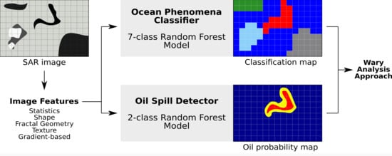
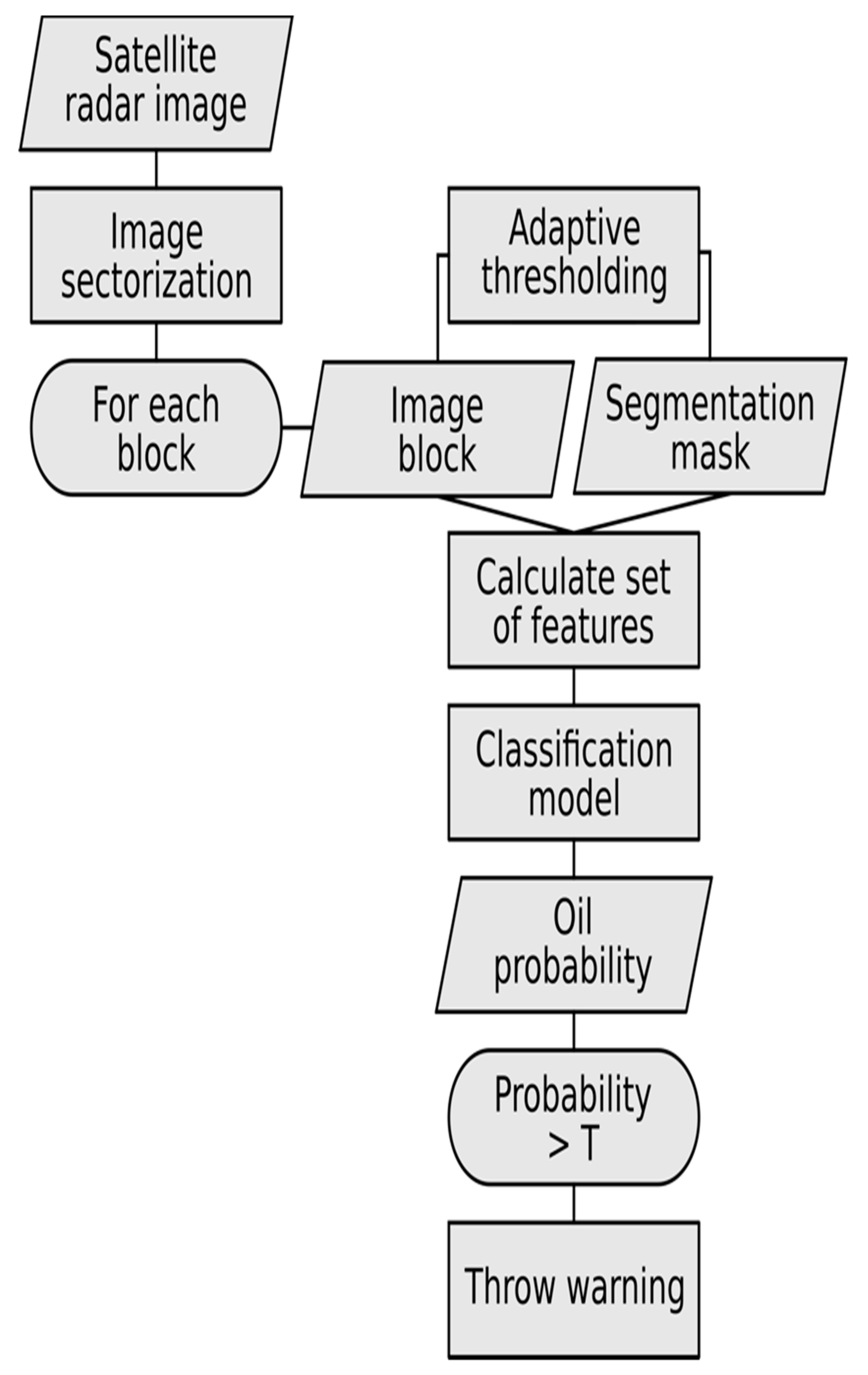
2.2. Image Classification Steps

This work was based on the methodology of [37], which had three main steps to oil spill detection: image segmentation, feature extraction, and classification. Our method initially uses the technique of separating the image into block, then applies a mixed adaptive thresholding segmentation to identify possible dark targets in the SAR images that will be later discussed. Adaptive thresholding algorithms are both simple and previously validated techniques [48] in oil spill segmentation. Subsequently, we performed the calculation of a set of image features for each given block and give them as input to a random forest model that was fitted to classify their associated block. The general classifier was trained to identify 7 classes: oil spill, biological film, rain cells, low wind regions, sea, ship presence, and terrain. On the other hand, the trained oil detector was a 2-class classifier and tried to predict oil probabilities in input data, being trained on 2 classes: oil spill and sea, the latter describing every image block that does not contain an oil spill. The features used to train both the classifiers and the detector’s random forest models were selected from 42 features belonging to 5 main categories: shape, complexity, statistical, gradient dependent, and textural features. These features were later reduced to 19 in order to eliminate data redundancy and unnecessary computational costs.
Image augmentation is a technique frequently used in machine learning. It is a process of slightly changing dataset images into a set of variations [49] before training or testing an algorithm, so that learning is maximized at each sample. In practice, applying this methodology multiplies the training and testing datasets to define more accurate models. The images used were rotated to 15, −30, 60, and −75° to apply the image augmentation concept and roughly quintuple our training and dataset testing.
After the training step, applying the classification methodology followed the so-called Radar Image Oil Spill Seeker (RIOSS) algorithm flow chart (Figure 1). An input SAR image was sectorized in blocks employing a pooling routine. For each block, dark regions were segmented, a set of features was computed, and an oil spill probability was calculated with the trained random forest model, and, if any block was given a higher oil probability than a pre-defined threshold value (T), the system operator received a warning.

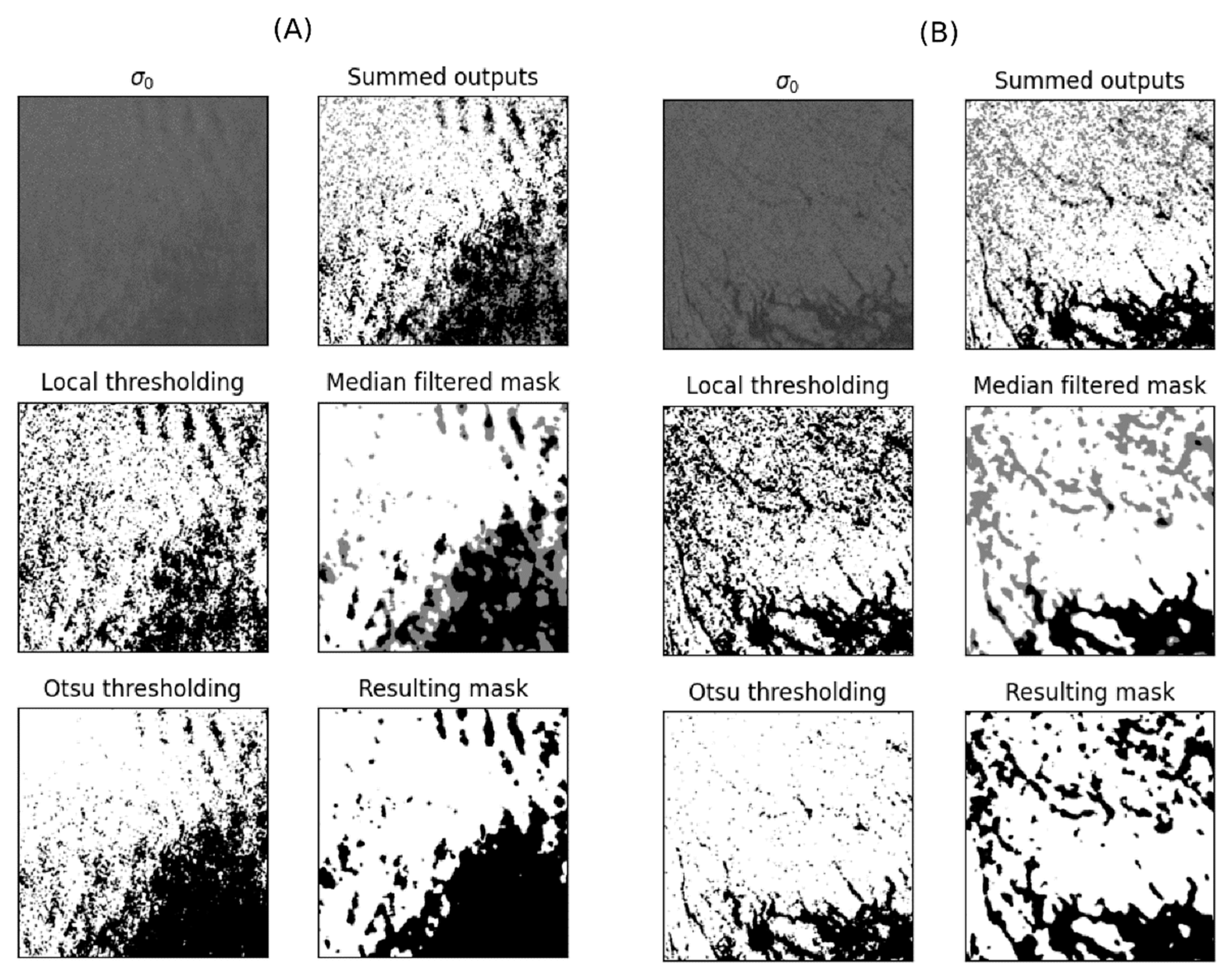
2.3. Image Segmentation

The black spot segmentation classified every image point in one of the two classes: foreground or background. The foreground class consisted of pixels belonging to oil spills and any look-alike phenomena, such as wind features, rain cells, and upwelling events. On the other hand, the background class encompassed the ocean’s sea surface, ships, terrain, and other features.
There are many two-class segmentation algorithms, the simplest one being global thresholding. A constant digital value is chosen as a threshold between classes (i.e., black and white pixels). Although functional, this algorithm has limitations in SAR image segmentation due to a significant gradient of digital values as the acquisition angles diverge from zenith. For this reason, many works choose reasonably more complex techniques, ranging from adaptive thresholding schemes [48] to convolutional neural network architectures [42], to accomplish this task.
The fast approach of adaptive thresholding methods was chosen, as segmentation was a second-order interest here. Two variants were combined into the segmentation solution: a cleaner one and a noisier mask. These two were then summed up, blurred, and applied to a final global thresholding. One of the binarization methods was the locally adaptive thresholding, which slid a window through the input image and returned a black pixel depending on its inner pixels’ mean and standard deviation. Two parameters were required: window size and a bias value multiplied by the standard deviation term of the threshold function, which controls how much local adaptation was wanted [50,51].
The other binarization method was the Otsu thresholding. This is a non-parametric, automatic binary clustering algorithm that maximizes inter-cluster variance in pixel values [51]. Both binarization algorithms were implemented in OpenCV, a C++ library built for real-time computer vision applications. After an extensive parameter search, local and Otsu thresholding were mixed when local thresholding used a window size of 451 × 451 pixels², and a bias value of 4 was used for the locally adaptive thresholding algorithm. The input images were low-passed filtered before segmentation for removing inconsistent data.

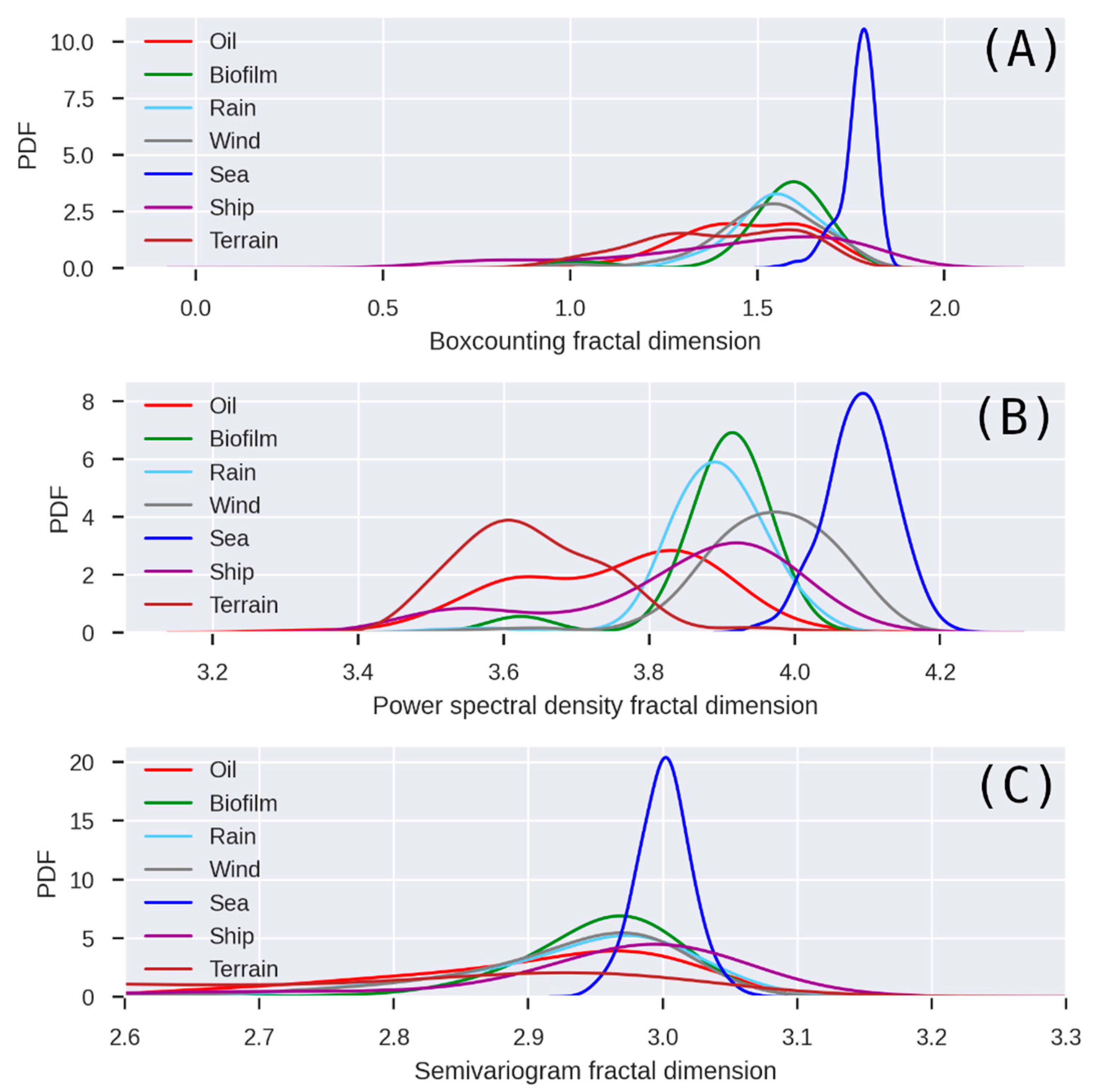
2.4. Feature Extraction and Selection

For classification, input SAR images were sectorized into blocks of 512 × 512 px². A big feature space with 42 elements was created from these blocks and divided into five main groups: statistics, shape, fractal geometry, texture, and gradient-based. The feature space is described in Table 1.
The authors of [20] showed how to calculate 2D gridded data fractal dimension from their power spectral density (PSD) amplitude decaying rate across the frequencies. In this work, we demonstrated fractal dimension distributions for images, with oceanographic features, using three different calculation methods: one from the PSD, as described by [20] and as a feature here abbreviated as psdfd; a second method used the basic box-counting technique described by [52], accounting for image self-similarity (bcfd); and the last method was a semivariogram based on fractal dimension, abbreviated as svfd, explored in the work of [53]. The latter method was computationally expensive to calculate raw data, so a heavy image resampling (to 5%) was applied before its evaluation. Another fractal geometry descriptor was lacunarity, which accounted for spatial gappiness distribution in an image. It was calculated via a box-counting algorithm, as previously used along with fractal dimension in a classification problem by [54] with satisfactory results.
Foreground and background average and standard deviations could not be calculated in some blocks of images when they had no foreground and background pixels. To continue using these features, such uncommon average and standard deviations were set as fixed constants, respectively, 0 and −1, to differ from the rest. Non-finite foregrounds to average background values were also set to −1. A small portion of blocks (1.3%) were associated with non-finite entropies. These values were chosen to be set to –1, ensuring the use of the feature. Lacunarity of segmentation masks and foreground-to-background standard deviations and skew ratios could not be calculated in most parts of the dataset (89%) as their denominators were frequently close to 0, leading to their feature space exclusion and therefore 39 elements remaining.
Data redundancy is a common phenomenon when one works with so many features; thus, a step was taken to filter them based on their absolute linear correlations and physical explainability. Similar features were grouped into high-value blocks around a hierarchical clustering diagonal and then applied to the features’ absolute correlation matrix. The hierarchical clustering implementation used was SciPy’s [55], using the Euclidean distance metric.

2.5. Decision Tree Classifiers

Decision tree classifiers were the basis for random forest classification models. A decision tree partitioned a feature space into class domains. It took a vector of features as input into its root node, then partitioned the tree into two branches, representing two different classes. It asked if one of the vector features was more significant than the node constant. The input vector then walked through its branch until reaching another node. There, one of its features was confronted again as being greater or lesser than a constant value. The input vector kept walking through its branches and nodes until it reached a leaf or final node, where the feature vector was finally classified between one of the considered classes.
Training a decision tree was carried out by choosing, for each of its partitioning nodes, the two splitting classes, the splitting feature and the splitting constant used. Sequentially, this process considered each feature and every two-class combination for each node and optimized a number, S, to be a constant that best split the part of the dataset that entered such a node in two classes. In practice, S was chosen so that the impurity measure (i.e., entropy or the Gini index) was minimized. The combination chosen for the node was the one that achieved minimum node impurity. The nodes were continually created until a maximum value or minimum impurity was acquired for each leaf. After training a decision tree, it is possible to measure feature importance to classification, as shown in [56].

2.6. Random Forest Classifiers

Random forests are bagging ensemble methods based on decision trees, first proposed by [45] and applied to remote sensing data by [57,58]. The idea behind these models is to generate many trees trained on random subsets of the dataset so that each tree node can only choose a feature from a random subset of m elements from the full features. The forest output is taken as the mode of its trees’ outputs. As decision trees are considered weak classifiers, meaning that they usually offer considerable variance, using many of them in random forests often generates robust, lower variance models. The author of [57] explained that the number of user-defined parameters in random forest classifiers was significantly less and more straightforward to define than other methods such as support-vector machines. Classification of feature importance can also be obtained from this model. This was performed by taking original dataset feature vectors, permuting one of the features to create unknown fake vectors, and passing both groups of vectors through the forest. The mean prediction error difference between the original and the fake vectors was taken as feature importance for each of the classes. Averaging these differences for all classes yielded an overall feature importance measure [56] as m = 6. Finally, RF models can predict classification probabilities from each tree’s predictions in the forest, which predict oil presence probability in SAR image sectors.

2.7. Metrics and Cross-Validation

After the models such as the random forests were trained, it was helpful to evaluate their correctness. This was carried out by defining metrics. Two of them were used here: accuracy and precision. When training a seven-label classifier, mean accuracy was chosen, as it has no intrinsic class bias. It is defined as a ratio between accurate predictions and the total number of predictions. It ranges from 0 (no correct predictions) to 1 (every prediction was correct). Although it was an effective metric, it was not the best one for an oil detector. It is much more dangerous to classify an oil image as a typical sea surface image than throwing a false positive alert, where the algorithm claims to have found oil but is actually looking at a clean sea surface image. For this reason, precision is a better metric in this case. Its definition is a ratio between accurate positive predictions (oil images predicted as oil) over every positive oil prediction (sum of correct sea and oil predictions). Optimizing our classification model through this metric biases it to the oil label. These metrics were defined in [59].
In order to validate our model, the k-fold method was used. This method split the dataset into k-groups and used each one of them once as data testing, which is used for evaluating the model after it is trained, while the remaining are joined and fed the model in training. Each of the trained models was evaluated based on the accuracy or precision of their respective data testing. The model’s metric was computed as an average of the calculated metrics. By proceeding this way, the model’s metric evaluation was always performed on untrained data to tell when overfitting occurred [60].

3. Results and Discussion

Black spot segmentation results can be seen in Figure 2. The Otsu thresholding tended to obtain cleaner results and delineates the darker regions of the images from the bright background well. In contrast, local thresholding could identify more subtle variations, although it was usually very noisy in this application. These remarks are seen in Figure 2A, where the top left region is captured with noise by local thresholding, while it is better chosen by Otsu’s method. In comparison, the top right oscillating features with lower contrast in the original image were better delineated by local thresholding than Otsu’s. The sum of the outputs and the median filter mask were used to calculate the target mask with oil. We have found out that by adding up both output and median filtering methods, the results gave more significant masks, as shown in both Figure 2A,B.
One thousand one hundred thirty-eight image blocks with 512 × 512 pixels were used to analyze the classification models’ features and training. This number was multiplied by rotating images and using them as new samples, usually called image augmentation, which increased our dataset’s size to 5125 images [61]. This number included 829 oil spills, 1002 biofilms, 454 rain cells, 1009 wind, 685 sea surface, 665 ships, and 1355 terrain images. While every image was used in the two-class problem, only a maximum of 700 images was used for each class to obtain a roughly balanced training set to the seven-class model and avoid higher bias values. For the feature selection part, the three different fractal dimension distributions can be seen in Figure 3. The semivariogram-based fractal dimension was applied to a 5% resampled version of the image array. The process could become operational, being the slowest routine with the highest computational cost in all stages of the project.
From all the considered fractal dimension estimators, the one that better separated the distribution peaks was calculated from the power spectral density function [20]. It was possible to observe the power spectrum-based fractal dimension’s PDF values with an acceptable separation between the target classes analyzed in the SAR image. The results showed good discrimination of oil spills from the sea surface, even without a detailed analysis of the backscatter coefficient. It allowed for a robust initial location of oil spills.
The semivariogram-based method showed the worst results for this application, as its distributions overlap more than the ones produced with other methods (Figure 3B). We understand that this behavior might be influenced by Dekker’s low sampling rate [62,63]. On the other hand, slight sampling changes did not sensibly transform the curves. Studying it across hundreds of images would require higher computational power, which is out of the scope of this investigation.
After data analysis, high redundancy was found in the 42 variables’ set. This dataset characteristic was minimized using the famous hierarchical clustering method, initially described by [63]. When applied to the absolute correlation matrix, it created blocks of correlated features around its principal diagonal (Figure 4).
The highly correlated variables in each block were excluded until the maximum feature-to-feature absolute correlation was below 80%. This process leads the correlation matrix to resemble an identity matrix (a zero-redundancy case). Therefore, in Table 2, we list the correlated features along with ones removed.
A way of visualizing so many features is by plotting their first two principal components, which together explain 40% of the dataset variance [64]. We could see that sea surface and terrain images form distinct clusters. Thus, contrastingly, rain, wind, biofilm, and ship feature domains overlap (Figure 5).
The Python machine learning library scikit-learn [65] implementations were used to create and train decision tree and random forest models. Both random forests had 60 decision trees and a max depth equal to 7 to avoid overfitting. For the seven-class (oil, biofilm, rain cell, wind, sea surface, ship, and terrain) image labeling problem, the decision tree and random forest models depicted an accuracy of 79% and 85%, respectively (right to total predictions ratio on test set). On the other hand, the oil detector (two-class problem) was evaluated with 86% precision (correct oil classifications to overall correct classifications on test set) by decision trees, while it yielded 93% when the random forest model was applied. The feature importance for the seven and the two-class problems can be seen in Figure 6. The confusion matrix from which the random forest models’ metrics were calculated are shown in Figure 7, normalized to predictions. The oil detector (Figure 7A) shows overall good results, as the low values off-diagonal show a low error rate. The seven-class labeler (Figure 7B) solves a more difficult task, experiencing the biggest problems when trying to identify biofilms and rain images from other look-alikes. As previously seen in Figure 5, oil-spill, biofilms, rain cells, and low wind conditions are very close. Rain cells are often correctly classified, yet many times other classes are misinterpreted as one of them. The classifier also misinterpreted some of the ship images as terrain, which can be explained by some images taken at ports with little land cover content.
We perceived that using just the 11 (out of 18) most important features for each model maintained their metrics. Moreover, 10 from these 11 features were almost the same in both models but with distinct internal importance: pseudo-spectral density function-based fractal dimension (psdfd), lacunarity (bclac), gradient mean (gradmean), mean, skewness (skew), Shannon entropy (entropy), kurtosis (kurt), segmentation mask’s Shannon entropy (segentropy), segmentation mask’s energy (segener), and background mean (bgmean). Other than that, the feature used was the foreground mean (fgmean) in the case of the seven-class model and complexity (complex) in the case of the oil detector.
A keynote here was that both models’ feature sets showed significant relevance to the attributes of pseudo-spectral density functions based on: fractal dimension (psdfd), lacunarity (bclac), gradient mean (gradmean), mean, skewness (skew), Shannon entropy (entropy), kurtosis (kurt), segmentation mask’s Shannon entropy (segentropy), segmentation mask’s energy (segener), and background mean (bgmean). On top of that, some classification methodologies were tested and validated, such as logistic regression, neural networks, fractal dimension, and the decision forest. Even with minor results, these methodologies helped us understand the backscattering mechanisms and how the spatial behavior of σ0 could affect the oil classification.
The seven-class feature classifier results can be seen in Figure 8. We can see that although there was noise in the classification output, the model could surely help an event interpretation in SAR images. Our algorithm correctly delineates the oil spill between various blocks classified as ocean waters but sometimes classifies blocks around the spills with a low wind label (gray, Figure 8D). Rain cells were also well highlighted. The ship that caused this accident near the Corsica island (2018) is also found (dark magenta) in the same image. Our model correctly identified the wind feature but had some classification noise, mainly in some blocks that resemble oil response or rain cells (Figure 8E). Along with some classification variance, our models dealt with the SAR image’s image borders, as there are noisier and invalid values present for both scanning method and geolocation reasons. This can affect some of the calculated features and, therefore, interferes with the random forest model’s behavior. A valid concern about the seven-class trained model was that it was biased not to classify rain cells correctly, as our dataset lacked enough images with these phenomena.
Our oil spill probability results can be seen on the oil spill images in Figure 9. The random forest detector algorithm was able to generalize oil spill responses compared to other image classes. The probability maps were close to zero on ocean sections, while it grew to higher values only in black-spotted positions with oil characteristics. The case in Figure 9A, where the central oil spot is highlighted by the algorithm (Figure 9C) and the case of the lower-sized oil portion at 43.5° N 9.45° E (Figure 9A), is successfully marked. Although probability was plotted, automated monitoring systems using this algorithm can set a probability threshold to warn an operator when an image is likely to present an oil spill. As the two-class model was already optimized with an oil-biased estimator (precision), the dataset unbalance, with a similar number of images for each class, was a minor setback. Contrarily, an authentic dataset critique is that it was mainly composed of enormous, catastrophic oil spill events. The produced oil detector had a bias towards classifying only major oil spills. Figure 9B shows other oil spill signature in the SAR image, while Figure 9D shows our models response when applied to it. The overall probability assessment over oil spills reveals good segmentation of the oil spill from the generated maps. It is clear from the examples shown that spot contours are more easily recognized than their central regions when the oil is significantly dispersed.
The random forest generated oil spill probability maps from images that do not contain oil spills are seen in Figure 10. The SAR images in Figure 10A,B show, respectively, rain and wind cells, while Figure 10C,D present their oil probability. These dark-spot look-alikes demonstrate similar SAR signature to oil spills but are still not highlighted by our model.
The selected attributes were cognitively detectable and could be later related to the imaged phenomena’s physical aspects. This process helped us apply the attributes to a random forest, increasing our algorithm’s accuracy and its ability to generate even more reliable results.

4. Conclusions

The occurrence of an oil spill in the ocean can make the incident almost uncontrollable due to the dynamics of the environment, reaching up hundreds of kilometers long, as occurred on the northeast coast of Brazil in 2019. Thus, the development of projects for identifying and monitoring oil spills on the ocean surface has scientific, economic, and environmental importance. Among the main difficulties described, we highlight the acquisition of reliable examples for training classifiers and the importance of adjusting contextual parameters for specific geographic areas. In this way, we developed and tested a set of open-source routines capable of identifying possible oil-like spills based on two random forest classifiers.
The first algorithm consists of an ocean SAR image classifier, labeling inputs as containing oil, biofilm, rain cell, wind, sea surface, ship, or terrain characteristics. This routine was developed with a classifier capable of circumventing the problems associated with look-alikes for a robust statistical analysis of the gradients associated with these features’ backscattering.
The second algorithm was developed to create an SAR image oil detector called Radar Image Oil Spill Seeker (RIOSS). RIOSS was responsible for identifying oil spill targets on marine surfaces using Sentinel-1 SAR images. Our aim was constituting an optimized feature space to serve as input to such classification models, both in terms of variance and computational efficiency. It involved an extensive search from 42 image attribute definitions based on their correlations and classifier-based importance estimative. Mixed adaptive thresholding was performed to calculate some of the features studied, returning consistent dark spot segmentation results.
In general, the model’s development suffered from dataset biases and other errors associated with the classification system. We observed that the general seven-class model was potentially affected by dataset unbalance, reducing the random forest’s effectiveness. Simultaneously, the oil detector managed to achieve compelling oil detection values on the marine surface (94% effectiveness). Being aware of these facts was crucial before implementing the automatic oil or other phenomena detection systems described here. There are several valuable improvements carried out in our methodology beyond its open-source characteristic: here, we deal with modern Sentinel-1 high resolution products, not only source codes but trained classification models, so that users do not need to develop their own dataset in further studies. Our system also lists an optimized set of interpretable image features, selected exactly for detecting oil spills from look-alikes. We propose a combined analysis approach, based on two models. One of them alarms about high oil spill probabilities, while the other points to the most probable look-alikes in case of a false positive. Such a tool provides the interpreter with useful information to better tackle ambiguous situations.
Our future challenges are dealing with boundaries and borders on SAR images on RIOSS. The absence of data in the external portions of a radar image still causes some pitfalls in our current version. We are currently working on tackling this problem. Concurrently, we are developing another code that will run in parallel with RIOSS that receives information about a possible oil occurrence, downloading wind and altimetry data from the Sentinel-3 satellite. This information is augmented by ocean current velocities, temperature, and salinity information from the Copernicus Marine Service sea surface Global Ocean Physics Analysis and Forecast (1/12°) model, which is updated daily. Understanding the ocean dynamics of a region impacted by an oil spill is essential for fast decision making to control the incidents.
Further studies are needed to classify oil spills by their nature and decomposition level, which can be carried out to deepen and improve our proposed methodology. Our idea is to keep the open-source code algorithm so that other works extend our study to various remote sensors to expand the tools and use RIOSS in studies of past oil spills. These future steps are part of an ongoing project recently funded by the Brazilian Navy; the National Council for Scientific and Technological Development (CNPQ); and the Ministry of Science, Technology, and Information (MCTI), call CNPQ/MCTI 06/2020—Research and Development for Coping with Oil Spills on the Brazilian Coast—Ciências do Mar Program, grant #440852/2020-0.

Author Contributions

Conceptualization, M.R.A.C. and L.F.F.d.M.; methodology, M.R.A.C. and L.F.F.d.M.; software execution, M.R.A.C. and L.F.F.d.M.; writing—original draft preparation, M.R.A.C. and L.F.F.d.M.; writing—review and editing, M.R.A.C., L.F.F.d.M., C.A.D.L., A.T.d.C.L., J.M.L., R.N.d.V., M.B.G. and M.J.P.; supervision, L.F.F.d.M., C.A.D.L. and A.T.d.C.L.; funding acquisition, A.T.d.C.L., C.A.D.L. and M.J.P. All authors have read and agreed to the published version of the manuscript.

Funding

This work is funded by the National Institute of Science and Technology–Petroleum Geophysics (INCT-GP) and MCTI/CNPQ/CAPES/FAPS Nº 16/2014 process 465517/2014-5, INCT PROGRAM and the additive projects entitled “Modeling, remote sensing, and preventive detection of oil/fuel accidents” and “Detection, control and preventive remediation of accidents involving the transportation of oil and fuels off the Brazilian coast” by MCTI/CNPQ/CAPES/FAPS 2019 and 2020, respectively. During this work, the following authors were supported by the National Council for Scientific and Technological Development (CNPQ) research fellowships: MRAC (grant #114259/2020-8), LFFM (CNPQ, process 424495/2018-0 and 380652/2020-0), CADL (grant #380671/2020-4), ATCL (grant #380653/2020-6), JML (CNPQ, process 381139/2020-4), RNV (grant #103189/2020-3), and MBG (grant #380461/2021-8). The first three authors would like to thank CNPQ for the financial support on the project entitled “Sistema de detecção de manchas de óleo na superfície do mar da bacia de Cumuruxatiba por meio de técnicas de classificação textural de imagens de radar e modelagem numérica” (Grant #424495/2018-0).

Institutional Review Board Statement

Not applicable.

Informed Consent Statement

Not applicable.

Data Availability Statement

Data available in a publicly accessible repository that does not issue DOIs. Publicly available datasets were analyzed in this study. The data analyzed in this manuscript are Sentinel-1 SAR images, made available at: “https://scihub.copernicus.eu/dhus/” (accessed on 27 March 2021). The routines used are openly available at: https://github.com/los-ufba/rioss (accessed on 27 March 2021).

Acknowledgments

We appreciate comments and suggestions from the anonymous reviewers that helped improve the quality and presentation of the manuscript.

Conflicts of Interest

The authors declare no conflict of interest.

References

  1. Celino, J.J.; De Oliveira, O.M.C.; Hadlich, G.M.; de Souza Queiroz, A.F.; Garcia, K.S. Assessment of contamination by trace metals and petroleum hydrocarbons in sediments from the tropical estuary of Todos os Santos Bay, Brazil. Braz. J. Geol. 2008, 38, 753–760. [Google Scholar] [CrossRef] [Green Version]
  2. Fingas, M. The Basics of Oil Spill Cleanup; Lewis Publisher: Boca Raton, FL, USA, 2001. [Google Scholar]
  3. Ciappa, A.; Costabile, S. Oil spill hazard assessment using a reverse trajectory method for the Egadi marine protected area (Central Mediterranean Sea). Mar. Pollut. Bull. 2014, 84, 44–55. [Google Scholar] [CrossRef]
  4. De Maio, A.; Orlando, D.; Pallotta, L.; Clemente, C. A multifamily GLRT for oil spill detection. IEEE Trans. Geosci. Remote Sens. 2016, 55, 63–79. [Google Scholar] [CrossRef]
  5. Franceschetti, G.; Iodice, A.; Riccio, D.; Ruello, G.; Siviero, R. SAR raw signal simulation of oil slicks in ocean environments. IEEE Trans. Geosci. Remote Sens. 2002, 40, 1935–1949. [Google Scholar] [CrossRef]
  6. Espedal, H.A.; Wahl, T. Satellite SAR oil spill detection using wind history information. Int. J. Remote Sens. 1999, 20, 49–65. [Google Scholar] [CrossRef]
  7. Fiscella, B.; Giancaspro, A.; Nirchio, F.; Pavese, P.; Trivero, P. Oil spill detection using marine SAR images. Int. J. Remote Sens. 2000, 21, 3561–3566. [Google Scholar] [CrossRef]
  8. Brekke, C.; Solberg, A.H.S. Oil spill detection by satellite remote sensing. Remote Sens. Environ. 2005, 95, 1–13. [Google Scholar] [CrossRef]
  9. Brekke, C.; Solberg, A. Classifiers and confidence estimation for oil spill detection in Envisat ASAR images. IEEE Geosci. Remote Sens. Lett. 2008, 5, 65–69. [Google Scholar] [CrossRef]
  10. Li, Y.; Li, J. Oil spill detection from SAR intensity imagery using a marked point process. Remote Sens. Environ. 2010, 114, 1590–1601. [Google Scholar] [CrossRef]
  11. Migliaccio, M.; Nunziata, F.; Montuori, A.; Li, X.; Pichel, W.G. Multi-frequency polarimetric SAR processing chain to observe oil fields in the Gulf of Mexico. IEEE Trans. Geosci. Remote Sens. 2011, 49, 4729–4737. [Google Scholar] [CrossRef]
  12. Migliaccio, M.; Nunziata, F.; Buono, A. SAR polarimetry for sea oil slick observation. Int. J. Remote Sens. 2015, 36, 3243–3273. [Google Scholar] [CrossRef] [Green Version]
  13. Salberg, A.B.; Rudjord, Ø.; Solberg, A.H.S. Oil spill detection in hybrid-polarimetric SAR images. IEEE Trans. Geosci. Remote Sens. 2014, 52, 6521–6533. [Google Scholar] [CrossRef]
  14. Kim, T.; Park, K.; Li, X.; Lee, M.; Hong, S.; Lyu, S.; Nam, S. Detection of the Hebei Spirit oil spill on SAR imagery and its temporal evolution in a coastal region of the Yellow Sea. Adv. Space Res. 2015, 56, 1079–1093. [Google Scholar] [CrossRef]
  15. Li, H.; Perrie, W.; He, Y.; Wu, J.; Luo, X. Analysis of the polarimetric SAR scattering properties of oil-covered waters. IEEE J. Sel. Top. Appl. Earth Obs. Remote Sens. 2015, 8, 3751–3759. [Google Scholar] [CrossRef]
  16. Singha, S.; Ressel, R.; Velotto, D.; Lehner, S. A combination of traditional and polarimetric features for oil spill detection using TerraSAR-X. IEEE J. Sel. Top. Appl. Earth Obs. Remote Sens. 2016, 9, 4979–4990. [Google Scholar] [CrossRef] [Green Version]
  17. Chen, G.; Li, Y.; Sun, G.; Zhang, Y. Application of deep networks to oil spill detection using polarimetric synthetic aperture radar images. Appl. Sci. 2017, 7, 968. [Google Scholar] [CrossRef]
  18. Vasconcelos, R.N.; Lima, A.T.C.; Lentini, C.A.; Miranda, G.V.; Mendonça, L.F.; Silva, M.A.; Cambuí, E.C.B.; Lopes, J.M.; Porsani, M.J. Oil Spill Detection and Mapping: A 50-Year Bibliometric Analysis. Remote Sens. 2020, 12, 3647. [Google Scholar] [CrossRef]
  19. Brown, C.E.; Fingas, M.F. New space-borne sensors for oil spill response. Int. Oil Spill Conf. Proc. 2001, 2001, 911–916. [Google Scholar] [CrossRef]
  20. Benelli, G.; Garzelli, A. Oil-spills detection in SAR images by fractal dimension estimation. IEEE Int. Geosci. Remote Sens. Symp. 1999, 1, 218–220. [Google Scholar]
  21. Marghany, M.; Hashim, M.; Cracknell, A.P. Fractal dimension algorithm for detecting oil spills using RADARSAT-1 SAR. In Proceedings of the International Conference on Computational Science and Its Applications, Kuala Lumpur, Malaysia, 26–29 August 2007; Springer: Berlin/Heidelberg, Germany, 2007; pp. 1054–1062. [Google Scholar]
  22. Marghany, M.; Hashim, M. Discrimination between oil spill and look-alike using fractal dimension algorithm from RADARSAT-1 SAR and AIRSAR/POLSAR data. Int. J. Phys. Sci. 2011, 6, 1711–1719. [Google Scholar]
  23. Del Frate, F.; Petrocchi, A.; Lichtenegger, J.; Calabresi, G. Neural networks for oil spill detection using ERS-SAR data. IEEE Trans. Geosci. Remote Sens. 2000, 38, 2282–2287. [Google Scholar] [CrossRef] [Green Version]
  24. Garcia-Pineda, O.; MacDonald, I.; Zimmer, B. Synthetic aperture radar image processing using the supervised textural-neural network classification algorithm. In Proceedings of the IGARSS 2008-2008 IEEE International Geoscience and Remote Sensing Symposium, Boston, MA, USA, 7–11 July 2008; Volume 4, p. 1265. [Google Scholar]
  25. Cheng, Y.; Li, X.; Xu, Q.; Garcia-Pineda, O.; Andersen, O.B.; Pichel, W.G. SAR observation and model tracking of an oil spill event in coastal waters. Mar. Pollut. Bull. 2011, 62, 350–363. [Google Scholar] [CrossRef] [PubMed]
  26. Singha, S.; Bellerby, T.J.; Trieschmann, O. Detection and classification of oil spill and look-alike spots from SAR imagery using an artificial neural network. In Proceedings of the 2012 IEEE, International Geoscience and Remote Sensing Symposium, Munich, Germany, 22–27 July 2012; pp. 5630–5633. [Google Scholar]
  27. Jiao, L.; Zhang, F.; Liu, F.; Yang, S.; Li, L.; Feng, Z.; Qu, R. A survey of deep learning-based object detection. IEEE Access 2019, 7, 128837–128868. [Google Scholar] [CrossRef]
  28. Yekeen, S.T.; Balogun, A.L.; Yusof, K.B.W. A novel deep learning instance segmentation model for automated marine oil spill detection. ISPRS J. Photogramm. Remote Sens. 2000, 167, 190–200. [Google Scholar] [CrossRef]
  29. Skøelv, Å.; Wahl, T. Oil spill detection using satellite based SAR, Phase 1B competition report. Tech. Rep. Nor. Def. Res. Establ. 1993. Available online: https://www.asprs.org/wp-content/uploads/pers/1993journal/mar/1993_mar_423-428.pdf (accessed on 27 March 2021).
  30. Vachon, P.W.; Thomas, S.J.; Cranton, J.A.; Bjerkelund, C.; Dobson, F.W.; Olsen, R.B. Monitoring the coastal zone with the RADARSAT satellite. Oceanol. Int. 1998, 98, 10–13. [Google Scholar]
  31. Manore, M.J.; Vachon, P.W.; Bjerkelund, C.; Edel, H.R.; Ramsay, B. Operational use of RADARSAT SAR in the coastal zone: The Canadian experience. In Proceedings of the 27th international Symposium on Remote Sensing of the Environment, Tromso, Norway, 8–12 June 1998; pp. 115–118. [Google Scholar]
  32. Kolokoussis, P.; Karathanassi, V. Oil spill detection and mapping using sentinel 2 imagery. J. Mar. Sci. Eng. 2018, 6, 4. [Google Scholar] [CrossRef] [Green Version]
  33. Konik, M.; Bradtke, K. Object-oriented approach to oil spill detection using ENVISAT ASAR images. ISPRS J. Photogramm. Remote Sens. 2016, 118, 37–52. [Google Scholar] [CrossRef]
  34. Xu, L.; Javad Shafiee, M.; Wong, A.; Li, F.; Wang, L.; Clausi, D. Oil spill candidate detection from SAR imagery using a thresholding-guided stochastic fully-connected conditional random field model. In Proceedings of the IEEE Conference on Computer Vision and Pattern Recognition Workshops, Boston, MA, USA, 7–12 June 2015; pp. 79–86. [Google Scholar]
  35. Marghany, M. RADARSAT automatic algorithms for detecting coastal oil spill pollution. Int. J. Appl. Earth Obs. Geoinf. 2001, 3, 191–196. [Google Scholar] [CrossRef]
  36. Shirvany, R.; Chabert, M.; Tourneret, J.Y. Ship and oil-spill detection using the degree of polarization in linear and hybrid/compact dual-pol SAR. IEEE J. Sel. Top. Appl. Earth Obs. Remote Sens. 2012, 5, 885–892. [Google Scholar] [CrossRef] [Green Version]
  37. Solberg, A.S.; Solberg, R. A large-scale evaluation of features for automatic detection of oil spills in ERS SAR images. In Proceedings of the IGARSS’96. International Geoscience and Remote Sensing Symposium, Lincoln, NE, USA, 31 May 1996; Volume 3, pp. 1484–1486. [Google Scholar]
  38. Solberg, A.S.; Storvik, G.; Solberg, R.; Volden, E. Automatic detection of oil spills in ERS SAR images. IEEE Trans. Geosci. Remote Sens. 1999, 37, 1916–1924. [Google Scholar] [CrossRef] [Green Version]
  39. Solberg, A.H.; Dokken, S.T.; Solberg, R. Automatic detection of oil spills in Envisat, Radarsat and ERS SAR images. In Proceedings of the IGARSS—IEEE International Geoscience and Remote Sensing Symposium, (IEEE Cat. No. 03CH37477). Toulouse, France, 21–25 July 2003; Volume 4, pp. 2747–2749. [Google Scholar]
  40. Solberg, A.H.; Brekke, C.; Husoy, P.O. Oil spill detection in Radarsat and Envisat SAR images. IEEE Trans. Geosci. Remote Sens. 2007, 45, 746–755. [Google Scholar] [CrossRef]
  41. Awad, M. Segmentation of satellite images using Self-Organizing Maps. Intech Open Access Publ. 2010, 249–260. [Google Scholar] [CrossRef] [Green Version]
  42. Cantorna, D.; Dafonte, C.; Iglesias, A.; Arcay, B. Oil spill segmentation in SAR images using convolutional neural networks. A comparative analysis with clustering and logistic regression algorithms. Appl. Soft Comput. 2019, 84, 105716. [Google Scholar] [CrossRef]
  43. Zhang, J.; Feng, H.; Luo, Q.; Li, Y.; Wei, J.; Li, J. Oil spill detection in quad-polarimetric SAR Images using an advanced convolutional neural network based on SuperPixel model. Remote Sens. 2020, 12, 944. [Google Scholar] [CrossRef] [Green Version]
  44. Castelvecchi, D. Can we open the black box of AI? Nat. News 2016, 538, 20. [Google Scholar] [CrossRef] [Green Version]
  45. Breiman, L. Random forests. Mach. Learn. 2001, 45, 5–32. [Google Scholar] [CrossRef] [Green Version]
  46. Olaya-Marín, E.J.; Francisco, M.; Paolo, V. A comparison of artificial neural networks and random forests to predict native fish species richness in Mediterranean rivers. Knowl. Manag. Aquat. Ecosyst. 2013, 409, 7. [Google Scholar] [CrossRef] [Green Version]
  47. De Zan, F.; Monti Guarnieri, A. TOPSAR: Terrain observation by progressive scans. IEEE Trans. Geosci. Remote Sens. 2006, 44, 2352–2360. [Google Scholar] [CrossRef]
  48. Mera, D.; Cotos, J.M.; Varela-Pet, J.; Garcia-Pineda, O. Adaptive thresholding algorithm based on SAR images and wind data to segment oil spills along the northwest coast of the Iberian Peninsula. Mar. Pollut. Bull. 2012, 64, 2090–2096. [Google Scholar] [CrossRef]
  49. Shorten, C.; Taghi, M.K. A survey on image data augmentation for deep learning. J. Big Data 2019, 6, 1–48. [Google Scholar] [CrossRef]
  50. Singh, T.R.; Roy, S.; Singh, O.I.; Sinam, T.; Singh, K. A new local adaptive thresholding technique in binarization. Arxiv Prepr. Arxiv 2012, 1201, 5227. [Google Scholar]
  51. Roy, P.; Dutta, S.; Dey, N.; Dey, G.; Chakraborty, S.; Ray, R. Adaptive thresholding: A comparative study. In Proceedings of the 2014 International conference on control, Instrumentation, communication and Computational Technologies, Kanyakumari, India, 10–11 July 2014. [Google Scholar]
  52. Li, J.; Qian, D.; Sun, C. An improved box-counting method for image fractal dimension estimation. Pattern Recognit. 2009, 42, 2460–2469. [Google Scholar] [CrossRef]
  53. Soille, P.; Jean-F, R. On the validity of fractal dimension measurements in image analysis. J. Vis. Commun. Image Represent. 1996, 7, 217–229. [Google Scholar] [CrossRef]
  54. Popovic, N.; Radunovic, M.; Badnjar, J.; Popovic, T. Fractal dimension and lacunarity analysis of retinal microvascular morphology in hypertension and diabetes. Microvasc. Res. 2018, 118, 36–43. [Google Scholar] [CrossRef]
  55. Virtanen, P.; Gommers, R.; Oliphant, T.E.; Haberland, M.; Reddy, T.; Cournapeau, D.; Van Mulbregt, P. SciPy 1.0: Fundamental algorithms for scientific computing in Python. Nat. Methods 2020, 17, 261–272. [Google Scholar] [CrossRef] [Green Version]
  56. Cutler, A.; Richard, D.C.; Stevens, J.R. Random forests. In Ensemble Machine Learning; Springer: Boston, MA, USA, 2012; pp. 157–175. [Google Scholar]
  57. Pal, M. Random forest classifier for remote sensing classification. Int. J. Remote Sens. 2005, 26, 217–222. [Google Scholar] [CrossRef]
  58. Gislason, P.O.; Benediktsson, J.A.; Sveinsson, J.R. Random forests for land cover classification. Pattern Recognit. Lett. 2006, 27, 294–300. [Google Scholar] [CrossRef]
  59. Fürnkranz, J.; Peter, A.F. An analysis of rule evaluation metrics. In Proceedings of the 20th international conference on machine learning (ICML-03), Washington, DC, USA, 21–24 August 2003. [Google Scholar]
  60. Fushiki, T. Estimation of prediction error by using K-fold cross-validation. Stat. Comput. 2011, 21, 137–146. [Google Scholar] [CrossRef]
  61. Shima, Y. Image augmentation for object image classification based on combination of pre-trained CNN and SVM. J. Phys. Conf. Series. Iop Publ. 2018, 1004, 012001. [Google Scholar] [CrossRef] [Green Version]
  62. Dekker, R.J. Texture analysis and classification of ERS SAR images for map updating of urban areas in the Netherlands. IEEE Trans. Geosci. Remote Sens. 2003, 41, 1950–1958. [Google Scholar] [CrossRef]
  63. Johnson, S.C. Hierarchical clustering schemes. Psychometrika 1967, 32, 241–254. [Google Scholar] [CrossRef]
  64. Fauvel, M.; Chanussot, J.; Benediktsson, J.A. Kernel principal component analysis for the classification of hyperspectral remote sensing data over urban areas. EURASIP J. Adv. Signal Process. 2009, 1–14. [Google Scholar] [CrossRef] [Green Version]
  65. Pedregosa, F.; Varoquaux, G.; Gramfort, A.; Michel, V.; Thirion, B.; Grisel, O.; Duchesnay, E. Scikit-learn: Machine Learning in Python. J. Mach. Learn. Res. 2011, 12, 2825–2830. [Google Scholar]
Figure 1. Flux diagram for RIOSS, the proposed automatic oil spill monitoring system.
Remotesensing 13 02044 g001
Figure 2. Segmentation methodologies applied in an SAR (σ0) image, according to the algorithms: local thresholding, the Otsu thresholding, summed outputs, and median filtered mask for Test Case 1 (A) and Test Case 2 (B).
Remotesensing 13 02044 g002
Figure 3. Probability density functions (PDFs), relative likelihood curves with the normalized area calculated for three different fractal dimension distributions: box counting (A), power spectral (B), and semivariogram (C).
Remotesensing 13 02044 g003
Figure 4. Dataset’s absolute correlation matrix with hierarchical clustering dendrograms.
Remotesensing 13 02044 g004
Figure 5. First two principal components’ scatter plot of the dataset, explaining 40% of its variance. Terrain and ocean images form distinct groups throughout the dataset, while oil and its look-alikes share roughly the same class domain.
Remotesensing 13 02044 g005
Figure 6. Random forest feature importance for the seven-label (A) and the oil detector (B) classification problems. Below (A) and (B), accumulated feature importance can be seen at (C) and (D). Error bars are feature importance standard deviations among the random forest’s trees.
Remotesensing 13 02044 g006
Figure 7. Confusion matrices for the oil detector (A) and the ocean feature classifier (B) random forest models.
Remotesensing 13 02044 g007
Figure 8. Oil spill (A), wind (B), and rain cell (C) images and their associated classified blocks as calculated from a 7-class random forest model in (D), (E), and (F).
Remotesensing 13 02044 g008
Figure 9. Oil spill images (A,B) and their associated oil presence probability as calculated from a two-class random forest detector model (C,D).
Remotesensing 13 02044 g009
Figure 10. Rain cell (A) and wind (B) images and their associated oil presence probability as calculated from a two-class random forest model (respectively, C and D). Although there were black spots in the SAR images, our algorithm did not associate these features with oil spills.
Remotesensing 13 02044 g010
Table 1. Features used grouped in five main categories, along with their acronyms and calculation description.
GroupFeatureAcronymCalculation
StatisticsImage meanmeanMean image value
Foreground meanfgmeanMean dark spot value
Background meanbgmeanMean background value
Image standard deviationstdImage value’s standard deviation
Foregrond standard deviationfgstdDark spot values’ standard deviation
Background standard deviationbgstdBackground values’ standard deviation
Image skewnessskewImage values’ skewness
Foreground skewnessfgskewForeground values’ skewness
Background skewnessbgskewBackground values’ skewness
Image kurtosiskurtImage values’ kutosis
Foreground kurtosisfgkurtDark spot values’ kurtosis
Background kurtosisbgkurtBackground values’ kurtosis
Foreground-to-background mean ratiofgobgmeanRatio between foreground and background means
Foreground-to-background standard deviation ratiofgobgstdRatio between foreground and background standard deviations
Foreground-to-background skewness ratiofgobgskewRatio between foreground and background skewnesses
Foreground-to-background kurtoses ratiofgobgkurtRatio between foreground and background kurtoses
Image Shannon entropyentropyShannon entropy calculated over the image
Segmentation mask’s Shannon entropysegentropyEntropy of the segmentation mask generated
ShapeForeground areafgareaDark spot area
Foreground perimeterfgperDark spot perimeter
Foreground perimeter-to-area ratiofgperoareaDark spot perimeter-to-area ratio
Foreground complexitycomplexP/√(4πA), where P and A are, respectively, the foreground’s perimeter and area
Foreground spreadingspreadλ2/(λ1 + λ2), where λ1 and λ2 are the two eigenvalues of the foreground coordinates’ covariance matrix and λ1 > λ2
Fractal geometryPower spectral density function-based fractal dimensionpsdfdFractal dimension as calculated by the image’s frequency components’ energy decay
Segmentation mask’s box-counting-based fractal dimensionbcfdFractal dimension as calculated by box counting
Semivariogram-based fractal dimensionsvfdFractal dimension as calculated from the image semivariogram
Box-counting-based lacunaritybclacImage lacunarity as calculated by box counting
Segmentation mask’s box-counting-based lacunaritysegbclacSegmentation mask’s lacunarity as calculated by box counting
TextureImage correlationcorrImage correlation from grey level co-occurrence matrix (GLCM)
Segmentation correlationsegcorrSegmentation mask correlation from GLCM
Image homogeneityhomoImage homogeneity from GLCM
Segmentation mask homogeneityseghomoSegmentation mask homogeneity from GLCM
Image dissimilaritydissImage dissimilarity from GLCM
Segmentation dissimilaritysegdissSegmentation mask dissimilarity from GLCM
Image energyenerImage energy from GLCM
Segmentation mask energysegenerSegmentation mask energy from GLCM
Image contrastcontImage contrast from GLCM
Segmentation contrastsegcontSegmentation mask contrast from GLCM
GradientMaximum image gradientgradmaxMaximum value of image gradient
Mean image gradientgradmeanMean value of image gradient
Median image gradientgradmedianMedian value of image gradient
Gradient mean to median ratiogradmeanomedianRatio between mean and median gradient values
Table 2. Correlated feature groups and selection performed. Both foreground (fgkurt) and background (bgkurt) kurtoses were removed, as they were always close to each other and showed no significant distinction among various image phenomena.
Correlated GroupMaintained FeaturesRemoved Features
1complexsegcorr, fgperoarea, fgper, seghomo, segcont, segdiss, bcfd
2entropyener, homo, gradmax, cont, diss
3Nonefgkurt, bgkurt
4gradmeangradmedian
5psdfdcorr, std, svfd, gradmeanomedian
6segentropyfgarea
Publisher’s Note: MDPI stays neutral with regard to jurisdictional claims in published maps and institutional affiliations.

