Article

Spatial Autocorrelation of Martian Surface Temperature and Its Spatio-Temporal Relationships with Near-Surface Environmental Factors across China’s Tianwen-1 Landing Zone

1
Chinese Antarctic Center of Surveying and Mapping, Wuhan University, Wuhan 430070, China
2
State Key Laboratory of Information Engineering in Surveying, Mapping and Remote Sensing, Wuhan University, Wuhan 430070, China
3
Shandong Provincial Key Laboratory of Optical Astronomy and Solar-Terrestrial Environment, Institute of Space Sciences, Shandong University, Weihai 264290, China
*
Author to whom correspondence should be addressed.
Remote Sens. 2021, 13(11), 2206; https://0-doi-org.brum.beds.ac.uk/10.3390/rs13112206
Submission received: 24 April 2021 / Revised: 27 May 2021 / Accepted: 30 May 2021 / Published: 4 June 2021
(This article belongs to the Special Issue Cartography of the Solar System: Remote Sensing beyond Earth)

Abstract

:
Variations in the Martian surface temperature indicate patterns of surface energy exchange. The Martian surface temperature at a location is similar to those in adjacent locations; but, an understanding of temperature clusters in multiple locations will deepen our knowledge of planetary surface processes overall. The spatial coherence of the Martian surface temperature (ST) at different locations, the spatio-temporal variations in temperature clusters, and the relationships between ST and near-surface environmental factors, however, are not well understood. To fill this gap, we studied an area to the south of Utopia Planitia, the landing zone for the Tianwen-1 Mars Exploration mission. The spatial aggregation of three Martian ST indicators (STIs), including sol average temperature (SAT), sol temperature range (STR), and sol-to-sol temperature change (STC), were quantitatively evaluated using clustering analysis at the global and local scale. In addition, we also detected the spatio-temporal variations in relations between the STIs and seven potential driving factors, including thermal inertia, albedo, dust, elevation, slope, and zonal and meridional winds, across the study area during 81 to 111 sols in Martian years 29–32, based on a geographically and temporally weighted regression model (GTWR). We found that the SAT, STR, and STC were not randomly distributed over space but exhibited signs of significant spatial aggregation. Thermal inertia and dust made the greatest contribution to the fluctuation in STIs over time. The local surface temperature was likely affected by the slope, wind, and local circulation, especially in the area with a large slope and low thermal inertia. In addition, the sheltering effects of the mountains at the edge of the basin likely contributed to the spatial difference in SAT and STR. These results are a reminder that the spatio-temporal variation in the local driving factors associated with Martian surface temperature cannot be neglected. Our research contributes to the understanding of the surface environment that might compromise the survival and operations of the Tianwen-1 lander on the Martian surface.

Graphical Abstract

1. Introduction

The Martian surface temperature can be used to diagnose processes occurring at and just below the surface of Mars. Moreover, an understanding of the near-surface Martian climate could help to determine whether the planet has the conditions to sustain life [1]. Surface temperature is one component of the near-surface climate, indicating the exchange and interaction of heat and momentum between the surface and the near-surface atmosphere [2]. Spatio-temporal variation in the Martian surface temperature could be used to infer the thermophysical properties and the physical processes occurring at the surface and the shallow subsurface [3]. Surface temperature is also relevant to Mars exploration missions, since the surface is the environment where a potential lander will operate; thus, the temporal and spatial variation range of the surface temperature must be considered in order to enable a lander to survive [4].
Since the 1970s, a large number of Mars exploration missions have been conducted to collect data about Mars, including climatic information. The National Aeronautics and Space Administration (NASA) and European Space Agency (ESA) have all vigorously pursued the study of the Martian surface temperature. Kieffer et al. (1976) drew a map of the global surface temperature of Mars based on the data from the Viking infrared thermal mapper, finding that the Martian surface temperature varies by region, day, and season [5]. This variation is related to the sunlight flux across seasons and geographical locations, as well as the physical properties of the near-surface geological materials, including grain size, rock abundance, and degree of exposed and hardened bedrock [6]. Many studies have noted temporal and spatial heterogeneity in the surface temperature of Mars [1,7,8,9]. Like the Earth, the surface temperature of Mars, and its changes, are not only spatially heterogeneous but also exhibit different levels of spatial coherence [10]. The consistency in temperature and temperature changes across a large geographical region means that the surface physical properties in this region of Mars are similar to those on Earth. Similarly, extreme weather on Mars can lead to adverse effects simultaneously across a large area.
In terms of meteorology and climate, the atmosphere of Mars is the closest to the Earth. It has a thin atmosphere (mainly composed of carbon dioxide, around 96% by volume [1]), and the rotation speeds and angles of inclination are similar Therefore, the meteorology and climate systems of the two planets have many qualitative similarities. The difference is that Mars is farther from the Sun, is smaller in size, has a thinner atmosphere, and is without liquid oceans, clouds, and other complex features such as a biosphere, which makes Mars quite different from Earth [1]. Furthermore, on Mars, the degree of spatial coherence of the surface temperature between different regions is not yet clear. Spatial autocorrelation measures the degree of spatial correlation based on the sample locations and sample values, and can reveal whether a spatial pattern expressed by the samples is a clustered, discrete, or random pattern [11,12]; it could be measured using Moran’s I index, a standard method to measure spatial autocorrelation, using the Global Moran’s I at the global scale [13] and the Local Moran’s I at the local scale [11]. Nevertheless, this spatial autocorrelation method has not been used to detect the spatial pattern of the Martian surface temperature, to the best of our knowledge.
The spatio-temporal variation in Martian surface temperature could be caused by multiple factors, such as the thermal inertia and albedo/emissivity of the surface materials, wind, dust, and topography. These influencing factors can also change with time and space. For example, dust storms at various scales on Mars are normal, and small (local) dust storms occur frequently, but large dust storms occur approximately once every three years, usually in the spring and summer in the southern hemisphere [14,15,16]. Spiga et al. (2011) found that on steep slopes with a low thermal inertia terrain, the effect of meso-scale winds on the surface temperature is particularly apparent [17]. Richardson et al. (2002) found that the huge topographical difference between the northern and southern hemispheres of Mars could lead to atmospheric circulation that to a large extent controls the transmission of water and large amounts of dust in the atmosphere between the hemispheres, which affects the Martian surface climate [18]. Some studies focused on the interaction between the atmosphere and the climate, finding that the cycle of C O 2 sublimation and condensation plays a major role in climate change [19,20,21]. Therefore, quantifying the changes in the temporal and spatial relationships between surface temperature and the influencing factors permits the prediction of future global and regional temperature trends on Mars.
Traditional regression models, such as ordinary least squares regression (OLS), yield estimated relationships that are stable in time and space, but these methods do not consider the spatial and temporal heterogeneity of variables, and a quantitative model is needed to estimate the spatial and temporal relationship between the Martian surface temperature and its potential influencing factors. A geographically and temporally weighted regression model (GTWR) can emphasize the non-stationarity of variables in time and space simultaneously, based on spatio-temporally weighted matrices [22]. Hence, this model could account for the spatio-temporal variation in the relationships between Martian surface temperature and the potential driving factors, and thus could be used to evaluate the driving factors affecting Martian surface temperature in various areas and time.
Our study provides a new perspective on the spatio-temporal distribution of the Martian surface temperature based on spatial autocorrelation analysis and a GTWR model. The Chinese Mars mission’s Tianwen-1 rover landed on Mars on 15 May 2021. The survival and work of the Martian lander on the surface is related to the temporal and spatial variation of the surface temperature of Mars. Our study was performed in the south of Utopia Planitia, the landing area of the Mars mission Tianwen-1. To characterize the Martian surface temperature, we selected three surface temperature indicators (STIs), including sol (sol represents a solar day on Mars), average temperature (SAT), sol temperature range (STR), and sol-to-sol temperature change (STC). The present study aims to (1) determine the degree of global and local spatial autocorrelation of STIs using the Global Moran’s I and Local Moran’s I; (2) quantitatively estimate the parameters that affect the spatio-temporal changes in STIs using the GTWR model; and (3) map the coefficients of each possible factor to demonstrate that the effects of the possible factors on the STIs are spatio-temporally heterogeneous.

2. Methods

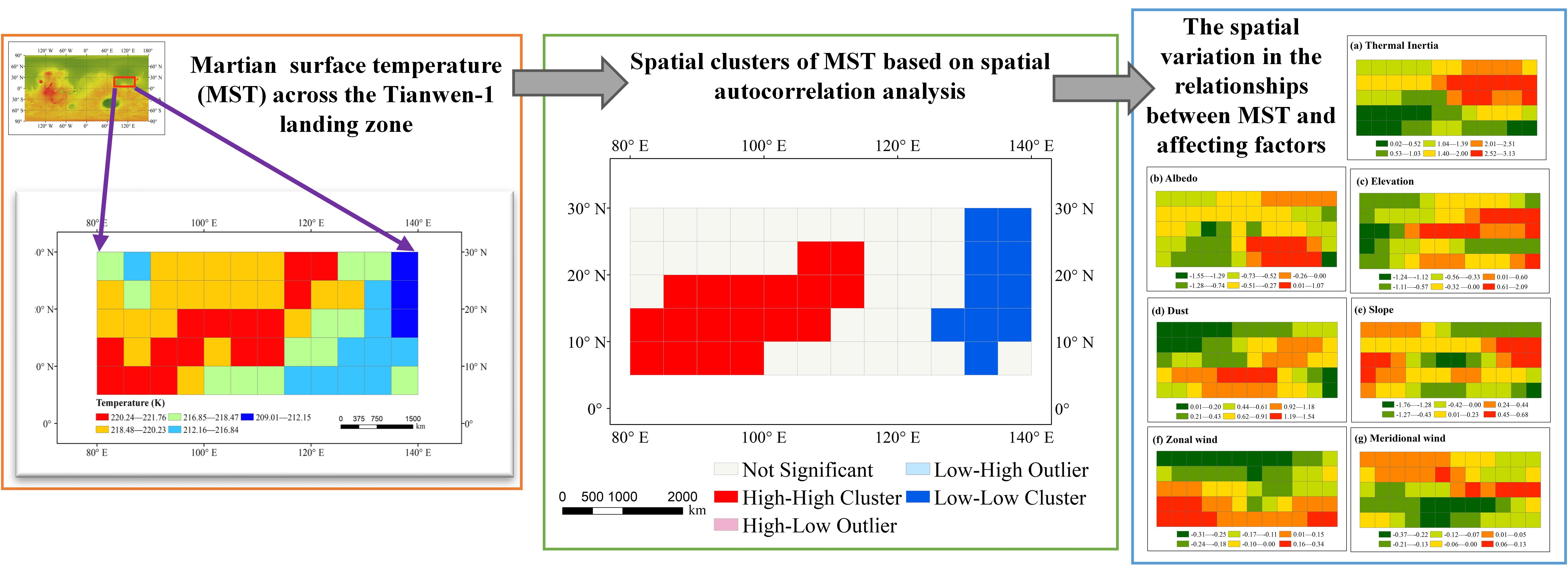
2.1. Study Area and Data Sources

The meteorological changes on the surface of Mars will have a great impact on the work of the Mars Landing Rover, so we chose the south of Utopia Planitia, the landing area for the China Mars Exploration Tianwen-1, as the study area of this research. Moreover, we expanded the compass of the study region to fully capture all the sites that the rover might traverse. As shown in Figure 1, the latitude of the study area ranged from 5° N to 30° and the longitude of the study area ranged from 80° E to 160 °   E. The northern part of the study area is in the Utopia Planitia, the eastern part is Isidis Planitia, and the southern part is Nepenthes Mensae.
The study area is divided into 34 geological units with a total of 12 geological types according to geological map of Mars from the U.S. Geological Survey (USGS) [23], as shown in Figure 2.
The surface has similar physical and chemical properties within a geological unit, such as the areas shown in Figure 2; thus, it can be used to explain the distribution of surface temperature. This research employed a 5° × 5° grid as the basic spatial unit to perform an empirical spatio-temporal analysis. The temporal range of analysis was the period corresponding to the landing time of the Tianwen-1 lander on Mars. Like the spatial range, we also extended this period appropriately as the research time range. The landing time was 15 May 2021. May 2021 on Earth corresponds to 81 sol to 111 sol of Martian year 36. Therefore, we conducted a spatio-temporal analysis of the surface temperature in the study area from 81 to 111 sols in each year from Martian year 29 to Martian year 32 (Martian year 29 to 32 corresponds to the Earth period from 7 December 2007 to 18 June 2015.). Three types of data were used in this study, including climate, topographic, and surface thermal attribute data.
The climate dataset, including surface temperature, dust, zone wind, and meridional wind during 81 sol to 111 sol in Martian year 29–32, was collected from the Open access to Mars Assimilated Remote Soundings (OpenMARS) database [24]. The climate data set has a temporal resolution of two Martian hours and a spatial resolution of five degrees of latitude and longitude. We calculated the surface temperature indicators (STIs), including sol average temperature (SAT), sol temperature range (STR), and sol-to-sol temperature change (STC), for each sol. The sol temperature range (STR) was defined as the difference between the maximum and minimum temperature of a Martian sol.
S T R t = T M A X t T M I N t
where S T R t represents the sol temperature range for sol t , and T M A X t and T M I N t represent the maximum temperature and minimum temperature for sol t , respectively.
The sol-to-sol temperature change (STC) is estimated as the difference between the sol average temperatures over two consecutive sol days.
S T C t = S A T t S A T t 1
where S T C t denotes the change in average sol temperature for the sol t , and S A T t and S A T t 1 denote the average sol temperature for the sol t and the previous sol t 1 , respectively.
The DEM (Digital Elevation Model) at 200 m resolution was obtained from Astrogeology PDS Annex, U.S. Geological Survey [25]. Based on the elevation data, the slope was extracted with the ArcGIS tool designed for this purpose. The surface thermal attributes data used in this study include surface thermal inertia and albedo. The nighttime surface thermal inertia (TI) map [26] with a resolution of 20 pixels per degree was selected from the Planetary Science Institute (https://sharad.psi.edu/inertia/ (accessed on 4 June 2021)). The surface albedo data [7] with a 7400 m resolution was obtained from the Astrogeology Science Center (https://astrogeology.usgs.gov (accessed on 4 June 2021)). A database with a 5 ° × 5 ° grid unit scale was constructed using the Zonal Statistics Tool in ArcGIS10.6. Python, R software, and Excel were used for data preprocessing and Geoda and ArcGIS10.6 for analysis and mapping.

2.2. Spatial Correlation Analysis

2.2.1. Global Spatial Correlation: Global Moran’s I

In order to explore whether the STIs of Mars at a certain location is affected by the STIs of its surroundings, we used spatial autocorrelation to estimate the spatial dependence. The Moran’s I index [13] is a standard method to measure spatial autocorrelation. It can assess the pattern of a data set spatially and evaluates whether the spatial pattern is dispersed, clustered, or random based on the geographical locations and attributes of the data. This study employed Moran’s I to explore whether the distribution of the Martian STIs (including SAT, TSR and TSG) is clustered or not. The expression for Moran’s I is described in Equation (3):
I = n i = 1 n j = 1 n w i j x i x ¯ x j x ¯ i = 1 n j = 1 n w i j i = 1 n x i x ¯ 2
where n is the number of geological units in the study area, x i and x j are the STI (SAT, STR and STC) values of the geological units at location i and j , respectively, x ¯ is the mean value of the STI, and w i j is the the spatial weight between the geological units at location i and j . Generally, when the geological unit i and geological unit j are adjacent, w i j = 1 ; when not adjacent, w i j = 0 .
The significance of the Moran’s I index is validated by a z-score and p-value. The z-score for the statistic is computed as
Z = I E I V I
where
E I = 1 / n 1
V I = E I 2 E I 2
In this study, the global Moran’s I was used to compute the degree of spatial autocorrelation in the whole study area based on 9999 permutations at the significance level p < 0.001. The range of Moran’s I index is (−1, 1). When the value of the Moran’s I > 0, it indicates that the STI shows a positive spatial correlation; that is, the pattern observed is clustered spatially, but the closer its value is to 1, the stronger the positive spatial correlation. When Moran’s I < 0, then the STI exhibits a spatially negative correlation; that is, the pattern observed is scattered or dispersed spatially, but the closer its value is to -1, the stronger the negative spatial correlation. When the value of the Moran’s I index is close to 0, it means that the STR is randomly distributed in space.

2.2.2. Local Spatial Correlation: Local Moran’s I

The Global Moran’s I Index can measure the degree of spatial autocorrelation across the whole study area, but there is usually heterogeneity in different geographic locations; thus, the degree of spatial autocorrelation is not stable locally. The Local Moran’s I [11] is a local extension of the Global Moran index, and used as a local indicator of spatial association (LISA). It can calculate the degree of spatial autocorrelation for every local location. Therefore, the Local Moran’s I for the STIs was employed to test whether the value of SAT, STR, and STC showed high–high (HH), low–low (LL), high–low (HL), or low–high (LH) spatial distribution patterns, which is expressed by Equation (7) [11]:
I i = x i x ¯ σ i 2 j = 1 , j i n w i j x j x ¯
where x i is the STI value for the geological unit at location i , x ¯ is the mean of the STI with the geological number n , and w i j is the spatial weight between the geological units at location i and j , and σ i 2 is the variance of x :
σ i 2 = j = 1 , j i n x j x ¯ 2 n 1 x ¯ 2
The z-score for the statistic is given by
Z i = Z i E I i V I i
where
E i = j = 1 , j i n w i j n 1
V I i = E I i 2 E I 2
In this study, the Local Moran’s I was employed to explore the spatial clusters and outliers of each of geological unit based on 9999 permutations with the significance level p < 0.001. A Local Moran’s I value > 0 indicates to the spatial unit under study that has similar STI values as its adjacent spatial unit, which are HH clusters or LL clusters. Two areas are defined to be adjacent if they share a border. When the Local Moran’s I value < 0 I, then the STI value of a spatial unit is quite different from its adjacent spatial units; these are the HL outliers and LH outliers.

2.3. Regression Models

2.3.1. Geographically Weighted Regression Model (GWR)

The Geographically Weighted Regression model (GWR) [27] is an extension of the traditional regression models, and can estimate the spatial non-stability of the regression parameters. The GWR model is expressed in Equation (12):
y i = β 0 u i , v i + k = 1 p β k u i , v i x i k + ϵ i
where y i denotes the value of the STI of geological i , u i , v i denotes the geographical location (latitude, longitude) of geological unit i ; β k u i , v i is the k th parameter of geological unit i , varying with the location of geological unit i ; β 0 u i , v i is the intercepts at a location u i , v i ; x i k is the value of the k th explanatory variable of the STI at location i ; and ϵ i is the error term.

2.3.2. Geographically and Temporally Weighted Regression Model (GTWR)

Although the GWR model can handle the spatial heterogeneity of the regression coefficients, it does not take temporal variation into consideration. Thus, Huang and Wu (2010) [28] proposed the geographically and temporally weighted regression model (GTWR) based on GWR, which manages both spatial and temporal heterogeneity The GTWR is described in Equation (13):
y i = β 0 u i , v i , t i + k = 1 p β k u i , v i , t i x i k + ϵ i
where y i is the value of the STI at location u i , v i at time t i ; u i , v i , t i denotes the spatial-temporal coordinate (latitude, longitude, time) of geological unit i at time   t i ; β k u i , v i , t i is the k th parameter of geological unit i , varying with both geographical location u i , v i and time t i ; β 0 u i , v i , t i represents the intercepts at a specific location u i , v i and time t i ; x i k is the value of the k th explanatory variable of STI at location i at time   t i ; and ϵ i is the error term.

3. Results

3.1. Descriptive Statistics of the Data

3.1.1. Spatial Heterogeneity of the Surface Temperature

We calculated the average temperature of the Tianwen-1 landing period (sol 81–111), corresponding to Martian years 29 to 32. Using these temperature data, we drew a surface temperature map to help understand the spatial pattern of the surface temperature in the study area. Figure 3 shows the average surface temperature during sol 81–111 from Martian years 29 to 32.
From Figure 3, we can see that the spatial distribution of the temperature was heterogeneous. The highest average temperature was 221.76 K, mainly distributed in the lHl geological unit (Figure 2) in the southwest. The lowest average temperature was 209.01 K found in the AHv geological unit (Figure 2) located in the northeast. This indicates that temperature is not stable in space; further research revealed that the surface temperature was also not stable in time.

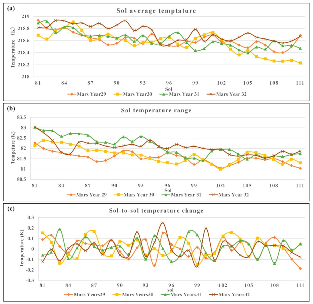
3.1.2. Temporal Temperature Trends

The Martian surface temperature not only shows spatial heterogeneity but also exhibits temporal variation. We describe the trends in three STIs over time. Figure 4 shows the change in sol average temperature (SAT), sol temperature range (STR), and sol-to-sol temperature change (STC) over time during the period sol 81–111 in Martian years 29–32.
As shown in Figure 4, all three temperatures varied with time. The SAT (Figure 4a) and STR (Figure 4b) decreased from 81 to 111 sols every Martian year. The SAT (Figure 4a) showed little change over time, ranging from 218.23 K (in sol 81 of Martian year 29) to 218.94 K (in sol 111 of Martian year 30). The temperature varied greatly in a sol, and the average STR in the study period was 81.84 K. The maximum STR was 83.03 K, appearing on the 81st sol of the 32nd Martian year, and the minimum STR was 81.00 K, appearing in the 102nd sol of the 30th Martian year. The STC fluctuated slightly over time (Figure 4c).

3.2. Spatial Correlation Diagnosis

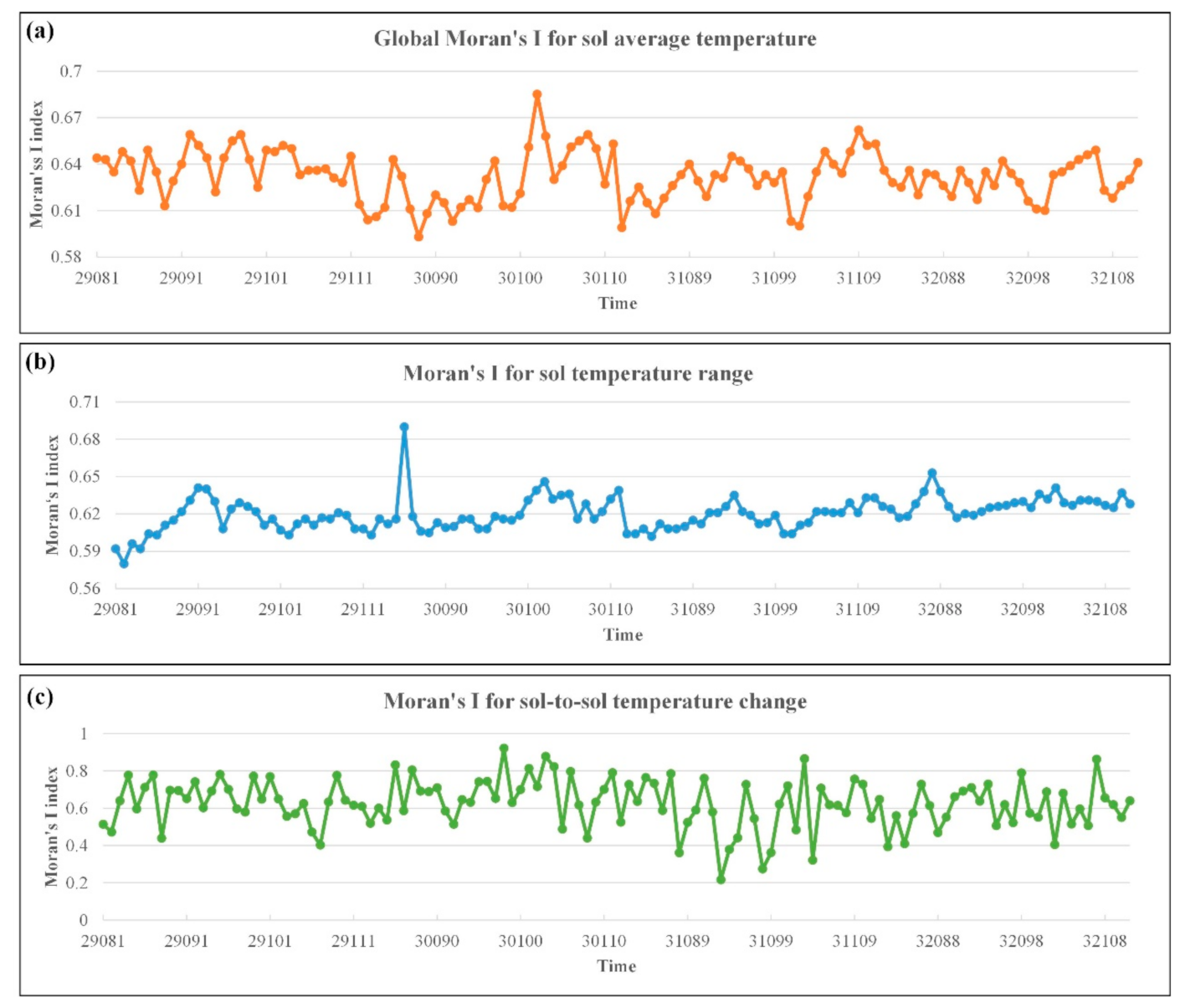
3.2.1. Global Moran’s I for Temperature

The Moran’s I was introduced to estimate the global spatial correlation for sol average temperature (SAT), temperature range (STR), and sol-to-sol temperature change (STC). The results of the Global Moran’s I for the SAT, STR, and STC during sol 81–111 from Martian years 29 to32 are shown in Figure 5.
As seen in Figure 5, the Moran’s I values of the three kinds of temperatures are all significant ( p < 0.001 ) and positive, indicating that the surface temperature was spatially correlated. Furthermore, the results of spatial correlation diagnosis indicate that the distribution of SAT, STR, and STC were not random, as their distribution displayed significant spatial aggregation.

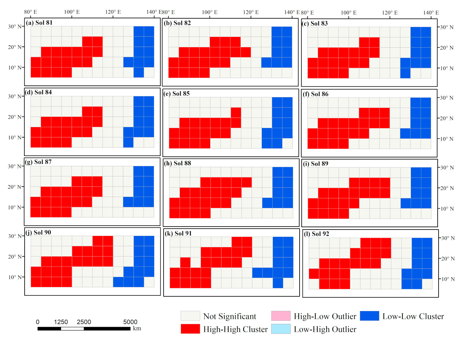
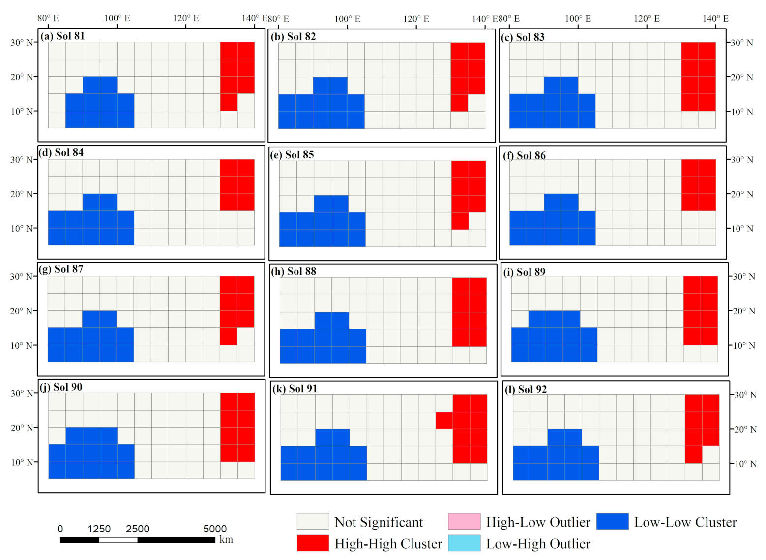
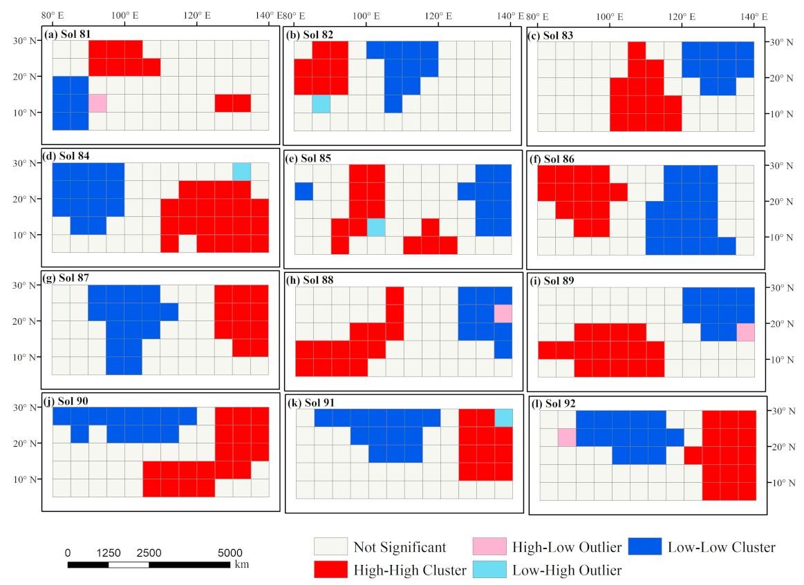
3.2.2. Local Moran’s I for Temperature

The Local Moran’s I was conducted to test for local spatial autocorrelation in the sol average temperature (SAT), temperature range (STR) and sol-to-sol temperature change (STC) during sol 81–111 from Martian years 29 to32 in the study area. We created agglomeration maps for SAT (Figure 6), STR (Figure 7), and STC (Figure 8) based on local indicators of spatial association (LISA) [11]. The agglomeration maps include high–high (HH), low–low (LL), high–low (HL), and low–high (LH) clusters.
In the SAT agglomeration map (Figure 6), the HH clusters refer to regions with high SAT surrounded by other regions with high SAT values. The HH SAT clusters are clearly visible and concentrated (Figure 6) in the southwestern part and central part of the study area, covering geological units including lHl, Ahi, eHt, mNh, and eHv. The LL SAT clusters, however, are distributed in the HNT, mNh and lAv geological units in the eastern part of the study area. The distribution of the SAT clusters was also related to topography. The HH clusters of SAT are distributed in relatively flat areas at a low elevation, while the LL clusters are located in areas of relatively steep terrain at a high elevation. The factors influencing this spatial pattern will be discussed in Section 3.3.
In the local spatial autocorrelation STR map (Figure 7), the HH clusters were defined as the regions with high STR surrounded by other regions with high STR (the definition is similar to those for LL, HL, and LH). The HH STR clusters are concentrated in the northeastern part of the study area, and the types of geological units covered by these areas mainly include Av, AHv, and lHl geologies. During the study period, the average atmospheric dust concentration in regions with HH STR clusters was relatively low. The distribution of the LL STR clusters is similar to that of the HH SAT clusters, mainly distributed in geological units lHl Ahi, eHv, and mNh in the southwestern region at a relatively low elevation. As shown in Figure 8, unlike the spatial clusters of SAT and STR that changed only slightly over time, the distribution of the STC clusters were scattered and changed significantly over time. These spatial aggregation patterns may be caused by multiple local factors. Based on this analysis, we applied a new model that considers spatial variations to explore the relationship between temperature and the affecting factors, instead of using the traditional models that only consider global correlations but neglect spatial variation. Thus, the GWR and GTWR models were selected to estimate the relationship between temperature and some potential affecting variables.

3.3. Temporal and Spatial Variation in the Relations between the STIs and Affecting Factors

Due to the different units of the impact factors of STIs in this study, we used the min–max feature scaling method to normalize the data to (0,1). A multi-collinearity test for each independent variable was performed before conducting GTWR; a stepwise regression analysis for all variables and selected variance inflation factor (VIF) test: when VIF > 7.5, there is multi-collinearity among the independent variables, as in other studies [29,30]. The results are shown in Table 1. The results show that the VIF value of each variable was less than 7.5. The mean VIF of the SAT group, STR group, and STC group was all 1.97. Therefore, the collinearity of all variables is not clearly apparent.
In order to explore the spatial-temporal heterogeneity, we applied four models, namely, ordinary least squares regression (OLS), temporally weighted regression (TWR), GWR, and GTWR, to select the optimal model for estimating the relations between the affecting factors and STIs (SAT, STR, and STC). The SAT, STR, and STC were taken as dependent variables, respectively, and the four models were used for regression analysis. We used R 2 , adjusted R 2 , and the Akaike information criterion (AICc) to compare the performance of OLS, TWR, GWR, and GTWR. The results are presented in Table 2.
As shown in Table 2, it is clear that the adjusted R 2 and R 2 value of the GTWR model were larger than that of the other three models (OLS, TWR, and GWR), and the AICc value of GTWR was smaller than that of the other models in each group. The GTWR model had the best model fit and outperformed the other tested regression models for each of the three groups of data in this study. Conversely, the global OLS model for SAT, ignoring the spatial and temporal variation, had an adjusted R 2 value of only 0.8430; the TWR model, ignoring temporal variation, has an adjusted R 2 value of only 0.8741; and the adjusted R 2 of GTWR increased to 0.9763. The GTWR model also had the best fit among the four regressions models for the STR and STC groups. The results show that the GTWR model is more accurate as both spatial heterogeneity and temporal variation were both taken into consideration. The adjusted R 2 and R 2 for the STC group were much lower than the SAT and STR groups. This may be explained in that the affecting factors for STC are different from those for SAT and STR, and the variables selected in this study may ignore the main affecting factors of STC. Thus, the SAT and STR were chosen as the dependent variables to further explore the spatial-temporal variation of the relationship between the STIs (SAT and STR) and affecting factors.

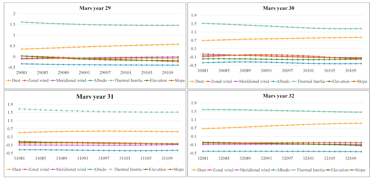
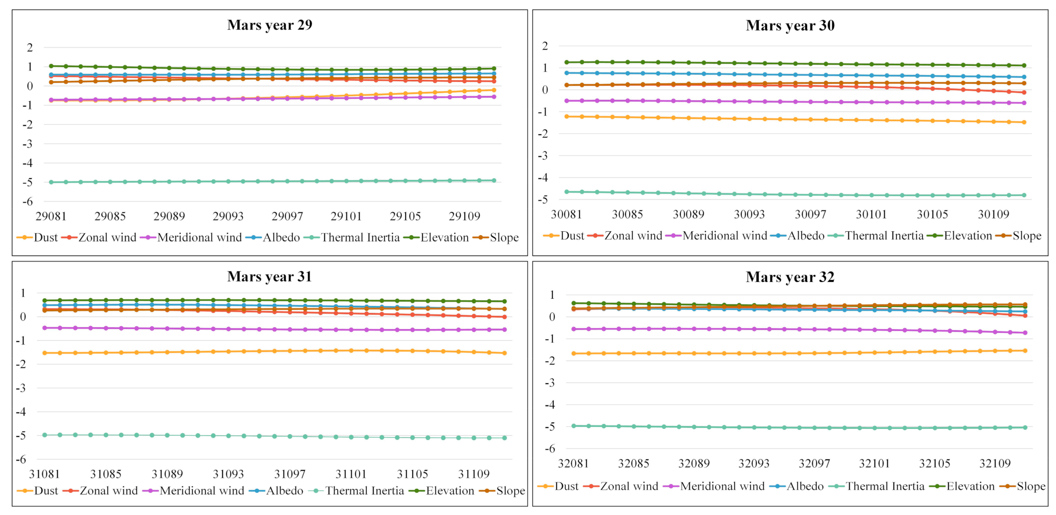
3.3.1. Temporal Trend in the Factors Affecting Temperature

The GTWR regression model considers the fluctuation in variables over time. The variation in the regression coefficients of each Martian sol over time based on the GTWR was obtained. We mapped the temporal trend for the coefficient of independent variables (albedo, thermal inertia, zonal wind, meridional wind, elevation, dust, and slope) for SAT (Figure 9) and STR (Figure 10) during 81–111 sol from Martian years 29 to 32.
The influence of thermal inertia and dust on SAT was positive during each Martian day during the study period (Figure 9). The effect of dust on temperature gradually increased from 81 to 111 Martian sol. The influence of thermal inertia on SAT gradually decreased from 81 to 111 sol, especially in Martian year 30, whereas the albedo, zonal wind, meridional wind, elevation, and slope had a relatively slight influence on SAT, and this influence was negative during most of the Martian sols. The influence of the affecting factors on STR was quite different from that on SAT, as shown in Figure 10.
As shown, the elevation, albedo, and slope had a positive effect on STR during the study period, and zonal wind also had a positive effect on STR on most Martian sols. The thermal inertia, dust, and meridional wind had a negative effect on STR. The influence of each factor on STR was relatively stable over Martian time during the study period.

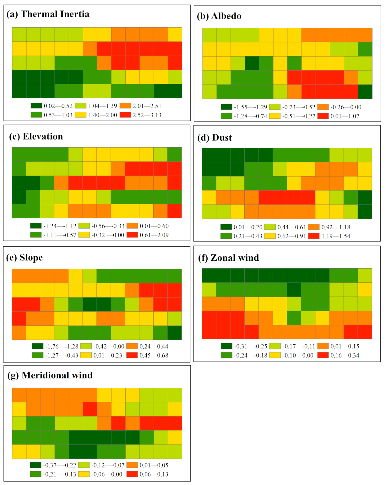
3.3.2. Spatial Variation in the Influence of the Factors Affecting Temperature

The surface temperature on Mars and its affecting factors are not stable in space, but spatially heterogeneous, and the relationship between them is also varied with geographic location. The GTWR model can estimate the local variation in the coefficient for each independent variable. The maps of the results showed that the effects of each factor on SAT (Figure 11) and STR (Figure 12) varied significantly in local areas.
As shown in the SAT distribution map—the affecting factor coefficients (Figure 11) and the SAT spatial autocorrelation map (Figure 6)—the HH clusters were greatly affected by the negative impact of albedo and elevation, while the LL clusters were greatly affected by the positive impact of thermal inertia and the negative impact of wind. Thermal inertia had a positive effect on SAT, especially in the northeastern part of the study area. The albedo had a negative correlation with the STR, except for the southeastern regions (Figure 11b). The elevation had a negative correlation on SAT in most area, especially the western part (Figure 11c). The relationship between dust and SAT was positive, and the influence gradually increased from north to south (Figure 11d). Slope has the greatest negative influence on the lHl and eHt geological units in the central and small parts of the south and north, while it has a positive influence on temperature in the east central and western region (Figure 11e). The relationship between zonal wind and SAT was positive in the south and negative in the north (Figure 11f). In contrast, the meridional wind exhibited a negative effect on SAT in the south, especially in the high-altitude south central region, while positive in the north (Figure 11e).
Unlike SAT, the thermal inertia had a negative correlation on STR across the study area, and the Av and AHv geological units with steep terrain and high elevation in the east have the greatest negative influence (Figure 12a). The influence of albedo on STR was negative in the southwestern region, and positive in the east (Figure 12b). Dust had a negative effect on STR in most areas except for some areas in the central region, and the negative effect was greatest in the southwest (Figure 12d). The LL clusters of STR (Figure 7) were greatly affected by the negative impact of albedo (Figure 12b) and dust (Figure 12d). Slope exhibited a great negative effect on the STR lHl and eHt geological units in the central, while other regions exhibited positive effects (Figure 12e). The reason for this difference can be explained by the sheltering effect of the mountains on both sides of the basin because the east, west, and south sides of the study area are surrounded by mountains. The relationship between meridional wind and STR was positive in the study area, and the degree of influence increased from north to south (Figure 12g).

4. Discussion

To deepen the understanding of the spatio-temporal variation of the surface temperature in the operating environment of the Mars Explore Mission Tianwen-1 lander, we used a spatial cluster analysis to verify three Martian STIs, including SAT, STR, and STC variations across the south of Utopia Planitia, the landing zones of the China Tianwen-1 Mars Exploration mission, during 81–111 Martian sols from Martian years 29 to 32. In addition, we estimated the spatio-temporal variations in the coefficients of the potential affecting factors that could account for the spatio-temporal distribution of SAT and STR. This is helpful to understand the driving factors and spatio-temporal differences in Martian surface temperature. This study could possibly support the construction of Martian climate models. This research was based on statistical models that we hope will encourage more process-based research on the spatial autocorrelation variation of Martian surface elements and their driving factors.
The distribution of SAT, STR, and STC in space and time were not stable, and exhibited clear signs of heterogeneity. Our research showed that although the distribution of SAT, STR, and STC varied with geographical location, their distribution is not random, but showed significant spatial aggregation, with average Global Moran’s I values of 0.632, 0.620, and 0.625. The local clusters of SAT and STR were relatively stable over time. The HH clusters of SAT concentrated in the southwestern part of the study area, and the SAT LL clusters were distributed in the northeast (Figure 6). The HH STR clusters were distributed in the northeastern part of the study area, and the LL STR clusters were mainly distributed in the southwest (Figure 7). In contrast to SAT and STC, the distribution of the STC clusters were scattered and changed significantly over time (Figure 8). The significant spatial aggregations of the STIs imply that the STIs and other potential factors affecting the STIs are not isolated, but have a certain degree of spatial correlation. Some Martian surface elements may also conform to Tobler’s first law of geography [31]; that is, everything is related to everything else, but near things are more related to each other.
The GTWR more accurately estimated the relationships between STIs and their driving factors with the greatest R 2 and adjusted R 2 , and the lowest AICc as compared with the OLS, TWR and GWR models. This is because these drivers are also heterogeneous in time and space, and the GTWR model captures the instability of the coefficients of the independent variables in time and space. Among all the independent variables, the influence of thermal inertia and dust on SAT and STR varied the most over time. The thermal inertia and dust had a positive relation with SAT in the whole study region. Conversely, in most areas of the study region, the thermal inertia as well as the dust coefficient affecting STR was negative, as the higher the surface thermal inertia and dust concentration, the smaller the sol temperatures range. This is consistent with conclusions of previous research. Gurwell et al. (2005) found that the average surface brightness temperature dropped by 20 K during the peak of a dust storm [32]. Because the surface of Mars is covered with different mixtures of dry boulders, sand, and dust, meteorological phenomena can lift dust particles into the atmosphere relatively easily. Dust particles suspended in the air increase the opacity of the atmosphere in the visible and thermal infrared bands. This opacity significantly weakens the sunlight radiation on the ground, resulting in a slower temperature rise during the day, and also causes the heating of the dust itself, and then the air is indirectly heated by contact with the dust, which keeps it warm at night, so the temperature difference between day and night is reduced.
However, in a small area in the central part, with a large altitude difference relative to the whole study area, the relationship between dust and STR was positive. The relative steep topography of these areas could account for this phenomenon. High elevation and slope can lead to local circulations that allow dust flowing day and night, so the relationship between dust and surface temperature in these areas is not consistent with that in flat areas. This topographic forced flow also affects the degree influence of the surface thermal inertia on STR, and the influence of thermal inertia on STR is intense at high-altitude regions.
We found that, in most places, the SAT exhibited negatively correlated with elevation, while STR was positively correlated with elevation. This may be related to the local atmospheric circulation caused by the topographical differences in the study area. Our conclusions were consistent with the atmospheric circulation caused by terrain differences in previous studies [18,33,34]. Like the Earth, topography has a great influence on climate. Millot et al. (2021) found that small-scale topography has a significant influence on the solar heating of the surface, causing the surface temperature change [35]. Solar heating varies day and night on the sloping terrain, causing buoyancy-driven circulation [1]. Since the thermal inertia of the atmosphere on Mars is lower than that of the Earth, the atmosphere responds faster to the surface heating of the Sun [36], so the local circulation on Mars is strong enough to remove dust from the surface [34]. During the day, unusual winds blow up the hillside, blowing dust from the edge of the cliff, pluming at the top of the mountain. At night, the cold descending wind flows down the slope and warm up as they descend to a higher pressure [1]. Our result showed that the surface temperature of the geological unit covered by AHv in the eastern region was greatly affected by the topography. This phenomenon lends supports for the conclusions drawn in previous studies [34,35], because a strong slope, wind, and local circulation often occur in this region, which is due to the large slope of this area and low thermal inertia (Figure S4).
Wind dominates the transportation of sediments on Mars [37]. Wind-blown sand, also known as saltation, often occurs on Mars, filling the atmosphere with dust aerosol. The dust aerosol in the atmosphere dominates the weather and climate of Mars [38]. Spiga et al. (2009) found that the descending wind at night can make the slopes of Mount Olympus 20 K warmer than the surroundings by constructing a three-dimensional model [39]. Our research results are consistent with this previous research showing that, except for parts of the north central regions, the meridional wind has a negative impact on the SAT in the study area. Both the SAT and STR in the south-central regions are most affected by wind, and these areas are also the most affected by dust. Because the elevation range in these areas are relatively large, the slope is relatively steep, so it is easy to cause local circulation; that is, slope wind leads to drastic surface temperature changes.

5. Conclusions

In this work, we used cluster analysis to verify the spatial aggregation of three surface temperature indicators (SAT, STR, and STC), and its variation in space and time at the southern Utopia, one of the Mars Mission Tianwen-1 landing zones. In addition, considering the heterogeneity of the driving factors over time and space, the GTWR model was introduced to explore the spatio-temporal dynamics of the relationships between the STIs (SAT and STR) and potential driving factors. Hence, this study addresses the following:
(1)
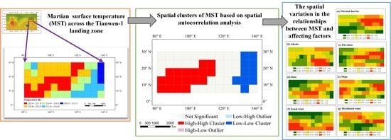
The distribution of SAT, STR, and STC was not random in space, but exhibited spatial aggregation characteristics. This indicates that the properties of multiple potential impact factors, including surface and near-surface features, may be very similar to those nearby, as inferred from these spatial clustering characteristics.
(2)
The spatial pattern of the SAT and STR clusters was relatively stable over time, but the distribution of STC clusters was scattered and changed significantly over time.
(3)
The temporal and spatial changes of the SAT and STR in the study area were affected by the variation in thermal inertia, albedo, dust, wind, and topography, and each factor showed signs of significant spatial and temporal heterogeneity. During the study period, the fluctuation of STIs with time was greatly affected by the variation in surface thermal inertia and dust.
(4)
Spatially, each factor has a different degree of positive or negative correlation with SAT and STR in different locations. Thermal inertia was greatly related to the spatial pattern of the STR, especially in the high-altitude regions. The east, west, and south sides of the study area are surrounded by mountains, thus the sheltering effect of the mountains on both sides of the basin caused the spatial differences in SAT and STR. The impact of each affecting factor on Martian STIs was not independent, but interactive. For example, the response of STIs to thermal inertia and dust in regions with a steep terrain was different from that in flat regions because local circulations are prone to form in steep regions compared with flat terrain regions, which causes dust to move more frequently in steep terrain regions.
These localized abnormal climate phenomena are detrimental to the accurate construction of climate models. We emphasize that regional and temporal differences are essential for understanding the process of Martian surface temperature changes. In the Martian climate simulation, if these temporal and spatial factors are not considered, the estimation will be biased. This work therefore provides information that could support the description of Martian regional climate changes in the future, and provides a reference for diagnosing the process occurring on the surface and shallow surface of China’s Mars Mission Tianwen-1 landing zone.
The limitations in this study should be mentioned. The influencing factors of the surface temperature indicators involved in this paper are not comprehensive. We have only focused on the most important variables affecting surface temperature, including thermal inertia, albedo, wind, dust, and topography factors, but the exact mechanisms that cause these changes on surface temperature are complex and not yet understood. We have done research on a local area of Mars, and whether the conclusions we reach are suitable for Mars globally remain to be further investigated. In addition, this study only analyzes the temporal and spatial characteristics of the STIs and their potential driving factors in the four Martian years during the time period corresponding to the Tianwen-1 landing. However, a long-term analysis of seasonal changes in surface temperature was not considered. In the future, we will study the spatio-temporal distribution of Martian surface temperature indicators and their influencing factors using a long-term series, including seasonal and inter-annual changes.

Supplementary Materials

The following are available online at https://0-www-mdpi-com.brum.beds.ac.uk/article/10.3390/rs13112206/s1, Figure S1: LISA map for sol average temperature (SAT) during sol 81–111 in Martian year 29–32, Figure S2: LISA for sol temperature range (STR) during sol 81–111 in Martian year 29–32, Figure S3: LISA for sol-to-sol temperature change (STC) during sol 81–111 in Martian year 29–32.

Author Contributions

Conceptualization, Y.L. and J.Y.; methodology, Y.L.; software, Y.L.; formal analysis, Y.L.; investigation, Y.L.; resources, Y.L.; data curation, Y.L.; writing—original draft preparation, Y.L.; writing—review and editing, Y.L., J.Y. and B.L.; visualization, Y.L.; supervision, F.L. and J.Y.; project administration, F.L. and J.Y.; funding acquisition, F.L. and J.Y. All authors have read and agreed to the published version of the manuscript.

Funding

This research was supported by the pre-research Project on Civil Aerospace Technologies (No. D020103); and the National Natural Science Foundation of China (42030110).

Data Availability Statement

The data we used in this study can be download from the OpenMars (https://ordo.open.ac.uk/collections/OpenMARS_database/4278950/1) (accessed on 4 June 2021), PDS (https://pds-geosciences.wustl.edu/) (accessed on 4 June 2021) and USGS center (https://www.usgs.gov/) (accessed on 4 June 2021).

Acknowledgments

We are grateful to NASA, ESA and OpenMars for providing models to make this research possible. We are also grateful to Stephen C. McClure for helping us improve the English language of this paper.

Conflicts of Interest
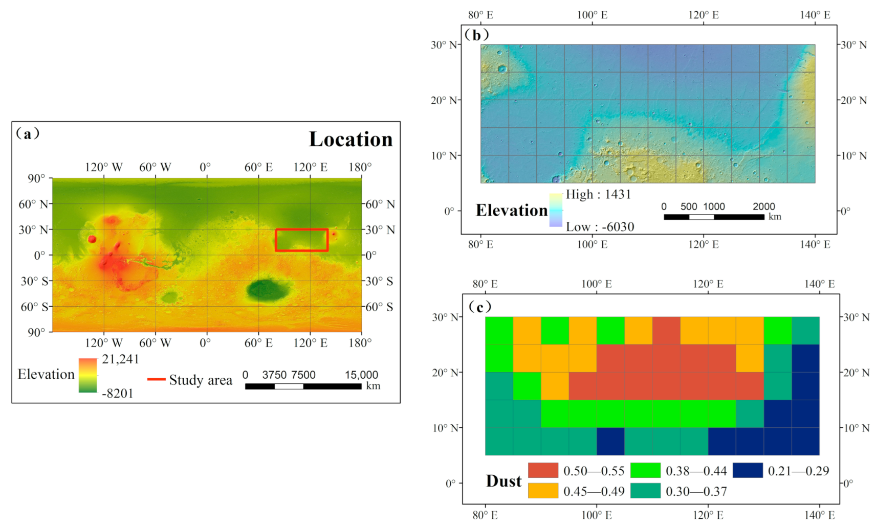
The authors declare no conflict of interest.

Appendix A

Description of the geological units used in this study.
Geological UnitDescription
AhiAmazonian and Hesperian impact unit—craters with rims and surrounding blankets; some include single to multi-lobed blanket forms, dense secondary crater chains, and (or) central peak or pit. Blanket thicknesses of meters to a few hundred meters. Upturned, ejected, and brecciated target rocks and sediments, with local areas of impact melt. Post-impact mass-wasting and fluvial-lacustrine and eolian infill of craters common.
AhvAmazonian and Hesperian volcanic unit—stacked, gently sloping lobate flows meters to tens of meters thick and hundreds of kilometers long. Variable daytime IR brightness in places. Cumulative thicknesses reach hundreds of meters to several kilometers. Flood lavas and large lava flows, undifferentiated, sourced from regional fissure and vent systems. Highly variable ages of individual flows, although generally younger in central parts of Tharsis rise
AvAmazonian volcanic unit—rugged, hummocky, and pitted fields of irregular, poorly defined flows forming plains hundreds to more than 1000 km across. Tens of meters, or more, thick.
HNtHesperian and Noachian transition unit—knobs, mesas, and intervening aprons and plains. May be tens to hundreds of meters thick. Noachian impact breccias, sediments, and volcanic deposits with intervening aprons of Hesperian mass-wasted materials.
eHtEarly Hesperian transition unit—plains-forming deposits, undulating to moderately rugged; includes scattered low knobs and mesas of Noachian highland material. May be tens to hundreds of meters thick. Largely unmodified flood lavas, including lava channels and other morphologies; sourced from fissures and shields
eHvEarly Hesperian volcanic unit—planar deposits meters to tens of meters thick and tens to hundreds of kilometers across; lobate scarps common. Variable daytime IR brightness in places. Hundreds of meters or more total thickness. Flood lavas, undifferentiated, sourced from regional fissure and vent systems.
eNhEarly Noachian highland unit—rugged, very high relief outcrops extending hundreds of kilometers. Thickness commonly exceeds a few kilometers but ill-defined. Undifferentiated impact, volcanic, fluvial, and basin materials. Heavily degraded; tectonically deformed in places.
lAvLate Amazonian volcanic unit—planar deposits containing lobate scarps that extend hundreds to more than 1000 km; sinuous troughs, ridges, and platy textures common; low-relief, shield-like edifices rare. Meters to tens of meters thick.
lHlLate Hesperian lowland unit—planar to undulating; lobate and troughed marginal areas in places. Hundreds of meters to kilometers thick. Fluvial/lacustrine/marine and colluvial sediments sourced from circum-lowland outflow channels and bounding highland terrains; likely intercalated with and underlain by lava and volcaniclastic rocks. Pervasively modified and obscured by periglaciation, sedimentary diapirism, and particulate mantling.
lHtLate Hesperian transition unit—plains-forming deposits, relatively smooth; includes small knobs and mesas of Noachian and perhaps younger material. May be tens to hundreds of meters thick.
mNhMiddle Noachian highland unit—uneven to rolling topography; high-relief outcrops that extend hundreds to thousands of kilometers. Commonly layered in crater walls. May be hundreds of meters to more than a kilometer thick. Undifferentiated impact, volcanic, fluvial, and basin materials. Moderately to heavily degraded.
mNhmMiddle Noachian highland massif unit—high-relief massifs tens of kilometers across separated by broad linear troughs and valleys. Ancient, degraded crustal rocks uplifted by large, basin-forming impacts. Dissected by basin-related fault structures and erosional valleys.

References

  1. Read, P.L.; Lewis, S.R.; Mulholland, D.P. The physics of Martian weather and climate: A review. Rep. Prog. Phys. 2015, 78, 125901. [Google Scholar] [CrossRef] [PubMed] [Green Version]
  2. Spanovich, N.; Smith, M.D.; Smith, P.H.; Wolff, M.J.; Christensen, P.; Squyres, S.W. Surface and near-surface atmospheric temperatures for the Mars Exploration Rover landing sites. Icarus 2006, 180, 314–320. [Google Scholar] [CrossRef]
  3. Tosi, F.; Capaccioni, F.; Capria, M.T.; Mottola, S.; Zinzi, A.; Ciarniello, M.; Filacchione, G.I.A.N.R.I.C.O.; Hofstadter, M.; Fonti, S.; Formisano, M.; et al. The changing temperature of the nucleus of comet 67P induced by morphological and seasonal effects. Nat. Astron. 2019, 3, 649–658. [Google Scholar] [CrossRef]
  4. Liu, J.; Zeng, X.; Li, C.; Ren, X.; Yan, W.; Tan, X.; Zhang, X.; Chen, W.; Zuo, W.; Liu, Y.; et al. Landing Site Selection and Overview of China’s Lunar Landing Missions. Space Sci. Rev. 2021, 217, 1–25. [Google Scholar] [CrossRef]
  5. Kieffer, H.H.; Chase, S.C.; Miner, E.D.; Palluconi, F.D.; Münch, G.; Neugebauer, G.; Martin, T.Z. Infrared thermal mapping of the martian surface and atmosphere: First results. Science 1976, 193, 780–786. [Google Scholar] [CrossRef] [PubMed]
  6. Presley, M.A.; Christensen, P.R. The effect of bulk density and particle size sorting on the thermal conductivity of particulate materials under Martian atmospheric pressures. J. Geophys. Res. 1997, 102, 9221–9229. [Google Scholar] [CrossRef]
  7. Christensen, P.; Bandfield, J.L.; Hamilton, V.E.; Ruff, S.; Kieffer, H.H.; Titus, T.N.; Malin, M.C.; Morris, R.V.; Lane, M.D.; Clark, R.L.; et al. Mars Global Surveyor Thermal Emission Spectrometer experiment: Investigation description and surface science results. J. Geophys. Res. 2001, 106, 23823–23871. [Google Scholar] [CrossRef]
  8. Hess, S.L.; Henry, R.M.; Leovy, C.B.; Ryan, J.A.; Tillman, J.E. Meteorological results from the surface of Mars: Viking 1 and 2. J. Geophys. Res. 1977, 82, 4559–4574. [Google Scholar] [CrossRef]
  9. Vasavada, A.R.; Piqueux, S.; Lewis, K.W.; Lemmon, M.T.; Smith, M.D. Thermophysical Properties Along Curiosity’s Traverse in Gale Crater, Mars, Derived from the REMS Ground Temperature Sensor. Icarus 2017, 284, 372–386. [Google Scholar] [CrossRef]
  10. Yang, H.; Piao, S.; Huntingford, C.; Peng, S.; Ciais, P.; Chen, A.; Zhou, G.; Wang, X.; Gao, M.; Zscheischler, J. Strong but Intermittent Spatial Covariations in Tropical Land Temperature. Geophys. Res. Lett. 2019, 46, 356–364. [Google Scholar] [CrossRef] [Green Version]
  11. Anselin, L. Local Indicators of Spatial Association—LISA. Geogr. Anal. 1995, 27, 93–115. [Google Scholar] [CrossRef]
  12. Dong, F.; Zhang, S.; Long, R.; Zhang, X.; Sun, Z. Determinants of haze pollution: An analysis from the perspective of spatio-temporal heterogeneity. J. Clean. Prod. 2019, 222, 768–783. [Google Scholar] [CrossRef]
  13. Moran, P.A.P. Notes on Continuous Stochastic Phenomena. Biometrika 1950, 37, 17–23. [Google Scholar] [CrossRef]
  14. Morgan, P.; Smrekar, S.E.; Lorenz, R.; Grott, M.; Kroemer, O.; Müller, N. Potential Effects of Surface Temperature Variations and Disturbances and Thermal Convection on the Mars InSight HP3 Heat-Flow Determination. Space Sci. Rev. 2017, 211, 277–313. [Google Scholar] [CrossRef]
  15. Kass, D.M.; Schofield, J.T.; Kleinböhl, A.; McCleese, D.J.; Heavens, N.G.; Shirley, J.H.; Steele, L.J. Mars Climate Sounder Observation of Mars’ 2018 Global Dust Storm. Geophys. Res. Lett. 2020, 47. [Google Scholar] [CrossRef]
  16. Cantor, B.A.; James, P.B.; Caplinger, M.; Wolff, M.J. Martian dust storms: 1999 Mars Orbiter Camera observations. J. Geophys. Res. 2001, 106, 23653–23687. [Google Scholar] [CrossRef]
  17. Spiga, A.; Forget, F.; Madeleine, J.-B.; Montabone, L.; Lewis, S.R.; Millour, E. The impact of martian mesoscale winds on surface temperature and on the determination of thermal inertia. Icarus 2011, 212, 504–519. [Google Scholar] [CrossRef]
  18. Richardson, M.I.; Wilson, R.J. A topographically forced asymmetry in the martian circulation and climate. Nature 2002, 416, 298–301. [Google Scholar] [CrossRef]
  19. Haberle, R.M.; Forget, F.; Colaprete, A.; Schaeffer, J.; Boynton, W.V.; Kelly, N.J.; Chamberlain, M.A. The effect of ground ice on the Martian seasonal CO2 cycle. Planet. Space Sci. 2008, 56, 251–255. [Google Scholar] [CrossRef]
  20. Acker, E.V.d.; Hoolst, T.V.; Viron Od Defraigne, P.; Forget, F.; Hourdin, F.; Dehant, V. Influence of the seasonal winds and the CO2 mass exchange between atmosphere and polar caps on Mars’ rotation. J. Geophys. Res. 2002, 107, 9-1–9-8. [Google Scholar] [CrossRef]
  21. Genova, A. ORACLE: A mission concept to study Mars’ climate, surface and interior. Acta Astronaut. 2020, 166, 317–329. [Google Scholar] [CrossRef]
  22. Fotheringham, A.S.; Crespo, R.; Yao, J. Geographical and Temporal Weighted Regression (GTWR). Geogr. Anal. 2015, 47, 431–452. [Google Scholar] [CrossRef] [Green Version]
  23. Tanaka, K.L.; Skinner, J.A., Jr.; Dohm, J.M.; Irwin, R.P., III; Kolb, E.J.; Fortezzo, C.M.; Platz, T.; Michael, G.G.; Hare, T.M. Cartographers. In Geologic Map of Mars; USGS: Reston, VA, USA, 2014. [Google Scholar]
  24. Holmes, J.A.; Lewis, S.R.; Patel, M.R. OpenMARS: A global record of martian weather from 1999 to 2015. Planet. Space Sci. 2020, 188, 104962. [Google Scholar] [CrossRef]
  25. Fergason, R.; Hare, T.; Laura, J.J.U.G.S. HRSC and MOLA Blended Digital Elevation Model at 200m v2, Astrogeology PDS Annex; US Geological Survey: Reston, VA, USA, 2018. [Google Scholar]
  26. Putzig, N.E.; Mellon, M.T. Apparent thermal inertia and the surface heterogeneity of Mars. Icarus 2007, 191, 68–94. [Google Scholar] [CrossRef]
  27. Brunsdon, C.; Fotheringham, A.S.; Charlton, M.E. Geographically weighted regression: A method for exploring spatial nonstationarity. Geogr. Anal. 1996, 28, 281–298. [Google Scholar] [CrossRef]
  28. Huang, B.; Wu, B.; Barry, M. Geographically and temporally weighted regression for modeling spatio-temporal variation in house prices. Int. J. Geogr. Inf. Sci. 2010, 24, 383–401. [Google Scholar] [CrossRef]
  29. Guo, B.; Wang, X.; Pei, L.; Su, Y.; Zhang, D.; Wang, Y. Identifying the spatiotemporal dynamic of PM2. 5 concentrations at multiple scales using geographically and temporally weighted regression model across China during 2015–2018. Sci. Total Environ. 2021, 751, 141765. [Google Scholar] [CrossRef]
  30. Sindayihebura, A.; Ottoy, S.; Dondeyne, S.; van Meirvenne, M.; van Orshoven, J. Comparing digital soil mapping techniques for organic carbon and clay content: Case study in Burundi’s central plateaus. Catena 2017, 156, 161–175. [Google Scholar] [CrossRef]
  31. Tobler, W.R. A Computer Movie Simulating Urban Growth in the Detroit Region. Econ. Geogr. 1970, 46, 234–240. [Google Scholar] [CrossRef]
  32. Gurwell, M.A.; Bergin, E.A.; Melnick, G.J.; Tolls, V. Mars surface and atmospheric temperature during the 2001 global dust storm. Icarus 2005, 175, 23–31. [Google Scholar] [CrossRef]
  33. Haberle, R.M.; Leovy, C.B.; Pollack, J.B. Some effects of global dust storms on the atmospheric circulation of Mars. Icarus 1982, 50, 322–367. [Google Scholar] [CrossRef]
  34. Richardson, M.I.; Newman, C.E. On the relationship between surface pressure, terrain elevation, and air temperature. Part I: The large diurnal surface pressure range at Gale Crater, Mars and its origin due to lateral hydrostatic adjustment. Planet. Space Sci. 2018, 164, 132–157. [Google Scholar] [CrossRef]
  35. Millot, C.; Quantin-Nataf, C.; Leyrat, C.; Enjolras, M. Local topography effects on the surface temperatures on Mars—Application to the case of Recurring Slope Lineae (RSL). Icarus 2021, 355, 114136. [Google Scholar] [CrossRef]
  36. Savijärvi, H.; Siili, T. The Martian slope winds and the nocturnal PBL jet. J. Atmos. Sci. 1993, 50, 77–88. [Google Scholar] [CrossRef]
  37. Sullivan, R.; Kok, J.F. Aeolian saltation on Mars at low wind speeds. J. Geophys. Res. 2017, 122, 2111–2143. [Google Scholar] [CrossRef]
  38. Kok, J.F. Difference in the wind speeds required for initiation versus continuation of sand transport on Mars: Implications for dunes and dust storms. Phys. Rev. Lett. 2010, 104, 074502. [Google Scholar] [CrossRef] [Green Version]
  39. Spiga, A.; Forget, F. A new model to simulate the Martian mesoscale and microscale atmospheric circulation: Validation and first results. J. Geophys. Res. 2009, 114, E2. [Google Scholar] [CrossRef] [Green Version]
Figure 1. The location of the study area (a), the elevation distribution (b), and the average dust distribution (c) during sol 81–111 from Martian year 29 to 32 across the study area.
Remotesensing 13 02206 g001
Figure 2. Geological map of the study area. A description of the geology units is listed in the Appendix A.
Remotesensing 13 02206 g002
Figure 3. The average surface temperature during sol 81–111 from Martian years 29 to 32.
Remotesensing 13 02206 g003
Figure 4. The change in sol average temperature (SAT), sol temperature range (STR), and sol-to-sol temperature change (STC) over time during the period sol 81–111 in Martian years 29–32.
Remotesensing 13 02206 g004
Figure 5. The trend in global spatial autocorrelation (p < 0.001) for sol average temperature (a), sol temperature range (b), and sol-to-sol temperature range (c) during sol 81–111 from Martian years 29 to 32 in the study area.
Remotesensing 13 02206 g005
Figure 6. LISA map for sol average temperature (SAT) during sol 81–92 in Martian year 29. The LISA maps for SAT during sol 81–111 from Martian year 29 to 32 are provided in the Supplementary Materials (Figures S1A–D).
Remotesensing 13 02206 g006
Figure 7. LISA for sol temperature range (STR) during sol 81–92 in Martian year 29. The LISA maps for STR during sol 81–111 from Martian years 29 to 32 are in the Supplementary Materials (Figures S2A–D).
Remotesensing 13 02206 g007
Figure 8. LISA for sol-to-sol temperature change (STC) during sol 81–92 in Martian year 29. The LISA maps for STC during sol 81–111 from Martian years 29 to 32 are in the Supplementary Materials (Figures S3A–D).
Remotesensing 13 02206 g008
Figure 9. The temporal trend in the coefficient of independent variables for SAT based on the GTWR model during 81–111 sol from Martian years 29 to 32.
Remotesensing 13 02206 g009
Figure 10. The temporal trend in the coefficient of independent variables for STR based on the GTWR model during 81–111 sol from Martian years 29 to 32.
Remotesensing 13 02206 g010
Figure 11. The distribution of the coefficients of the affecting factors (thermal inertia (a), albedo (b), elevation (c), dust (d), slope (e), zonal wind (f), and meridional wind (g) for SAT.
Remotesensing 13 02206 g011
Figure 12. The distribution of the coefficients of the affecting factors (thermal inertia (a), albedo (b), elevation (c), dust (d), slope (e), zonal wind (f) and meridional wind (g) for STR.
Remotesensing 13 02206 g012
Table 1. Stepwise regression multicollinearity test results.
Dependent VariablesIndependent VariablesCoefficientp-ValueVIF
SATDust0.3090.000 1.449
Zonal wind−0.0750.000 1.037
Meridional wind−0.0220.000 1.097
Albedo−0.1840.000 1.865
Thermal Inertia0.6530.000 1.347
Elevation−0.1120.000 4.118
Slope−0.0090.234 2.886
STRDust−0.0610.000 1.449
Zonal wind0.0530.000 1.037
Meridional wind−0.2050.000 1.097
Albedo0.1120.000 1.865
Thermal Inertia−0.8800.000 1.347
Elevation−0.1070.000 4.118
Slope0.0860.000 2.886
STCDust−0.0040.765 1.449
Zonal wind0.0320.006 1.037
Meridional wind0.0910.000 1.097
Albedo0.0140.374 1.865
Thermal Inertia0.0650.000 1.347
Elevation0.1430.000 4.118
Dust0.3090.000 1.449
Table 2. Performance of the OLS, TWR, GWR, and GTWR models.
Dependent VariablesModels Adjusted   R 2 R 2 AICc
Sol average temperatureOLS0.8430 0.8430 5199.40
TWR0.8741 0.8746 4992.49
GWR0.9721 0.9722 2253.13
GTWR0.9763 0.9764 2047.37
Sol temperature rangeOLS0.8410 0.8410 9935.14
TWR0.8560 0.8565 9834.79
GWR0.9814 0.9815 6102.64
GTWR0.9830 0.9821 6022.73
Sol-to-sol temperature changeOLS0.0280 0.0280 −1402.83
TWR0.1015 0.1049 −1486.42
GWR0.0700 0.0735 −1430.49
GTWR0.2271 0.2300 −1580.30
Publisher’s Note: MDPI stays neutral with regard to jurisdictional claims in published maps and institutional affiliations.

