
A Random Forest-Based Data Fusion Method for Obtaining All-Weather Land Surface Temperature with High Spatial Resolution


1
State Key Laboratory of Remote Sensing Science, Jointly Sponsored by Beijing Normal University and Institute of Remote Sensing and Digital Earth of Chinese Academy of Sciences, Beijing 100875, China
2
Institute of Remote Sensing Science and Engineering, Faculty of Geographical Science, Beijing Normal University, Beijing 100875, China
3
Shaanxi Key Laboratory of Earth Surface System and Environmental Carrying Capacity, College of Urban and Environmental Science, Northwest University, Xi’an 710127, China
*
Author to whom correspondence should be addressed.
Remote Sens. 2021, 13(11), 2211; https://0-doi-org.brum.beds.ac.uk/10.3390/rs13112211
Submission received: 28 April 2021
/
Revised: 2 June 2021
/
Accepted: 3 June 2021
/
Published: 5 June 2021
(This article belongs to the Special Issue Fusion of High-Level Remote Sensing Products)
Abstract
:Land surface temperature (LST) is an important parameter for mirroring the water–heat exchange and balance on the Earth’s surface. Passive microwave (PMW) LST can make up for the lack of thermal infrared (TIR) LST caused by cloud contamination, but its resolution is relatively low. In this study, we developed a TIR and PWM LST fusion method on based the random forest (RF) machine learning algorithm to obtain the all-weather LST with high spatial resolution. Since LST is closely related to land cover (LC) types, terrain, vegetation conditions, moisture condition, and solar radiation, these variables were selected as candidate auxiliary variables to establish the best model to obtain the fusion results of mainland China during 2010. In general, the fusion LST had higher spatial integrity than the MODIS LST and higher accuracy than downscaled AMSR-E LST. Additionally, the magnitude of LST data in the fusion results was consistent with the general spatiotemporal variations of LST. Compared with in situ observations, the RMSE of clear-sky fused LST and cloudy-sky fused LST were 2.12–4.50 K and 3.45–4.89 K, respectively. Combining the RF method and the DINEOF method, a complete all-weather LST with a spatial resolution of 0.01° can be obtained.

1. Introduction
Land surface temperature (LST) is an important indicator of energy balance and material exchange on the surface of the Earth, and has been widely used in many fields [1,2,3,4,5]. With the advancement of remote sensing technology and the stimulus of strong application demands, the number of Earth observation satellites has increased rapidly, producing a massive amount of satellite data [5]. Various advanced LST products can be generated from these satellite data [6]. However, due to cloud contamination, and defects of the retrieval algorithms, advanced remote sensing (RS) products derived from single sensors are suspected to have spatial incompleteness, temporal discontinuity, and inconsistent physical meanings [7]. In contrast, the spatial integrity and data quality of the same products derived from multisensory observations may be complementary. For example, satellite-retrieved LST includes thermal infrared (TIR) LST and passive microwave (PMW) LST. The TIR LST data have high spatial resolution (e.g., 1 km for Moderate Resolution Imaging Spectroradiometer (MODIS) LST) and high retrieval accuracy (approximately 0.3–2 K), but there are many missing values in the data due to clouds [8,9,10,11,12,13]. PMW radiation can penetrate clouds, but PMW LST data have a relatively low spatial resolution (e.g., 25 km for Advanced Microwave Scanning Radiometer–Earth Observing System (AMSR-E) LST) and relatively low accuracy (approximately 3–6 K) [14,15,16]. Therefore, the TIR LST data and the PMW LST data are complementary in terms of spatiotemporal completeness and data accuracy. Therefore, the fusion of TIR and PMW LST data has become a promising method for obtaining high-quality all-weather RS products [17,18].
Current TIR and PMW LST fusion methods include the cloud proportional weighting method, the temperature spatiotemporal interpolation method, the temporal component decomposition method, the Bayesian maximum entropy (BME) method, the machine learning method, and the hybrid method [19,20,21,22,23,24,25,26,27,28]. Although the ML method has high requirements for computing power and storage capacity, compared with other methods, it has excellent performance and generalization ability [29]. As the ML method is good at characterizing the relationship between environment variables and dependent variables, it is often used to simulate the relationship between LST and other variables [30,31,32]. With the latest developments and innovations in the computing field, the cloud computing capabilities, high-performance computing capabilities and storage capabilities have increased, which facilitates and supports data fusion using ML methods [33]. In this context, it is of great significance to improve the efficacy and flexibility of ML methods to generate advanced RS products on the regional or global scale.
The random forest (RF) model proposed by Breiman is a commonly used method in ML and has been widely used due to its high accuracy and flexibility [34]. The RF method can effectively use auxiliary data to improve the accuracy of fusion results, but the traditional RF method often does not consider the spatial information of RS data [35]. However, because RS variables often have spatial heterogeneity, the potential relationship between the independent and dependent variables in RF can vary spatially [36,37]. Therefore, for RS data, models built using regression approaches that ignore the spatial structure of RS data may not have sufficient predictive prowess.
Therefore, we sought to add spatial information to the RF model for spatial calibration, to compare this model with a model without spatial information to select the best RF model, and finally to predict all-weather LST data with high spatial resolution.
2. Study Area and Data
2.1. Study Area
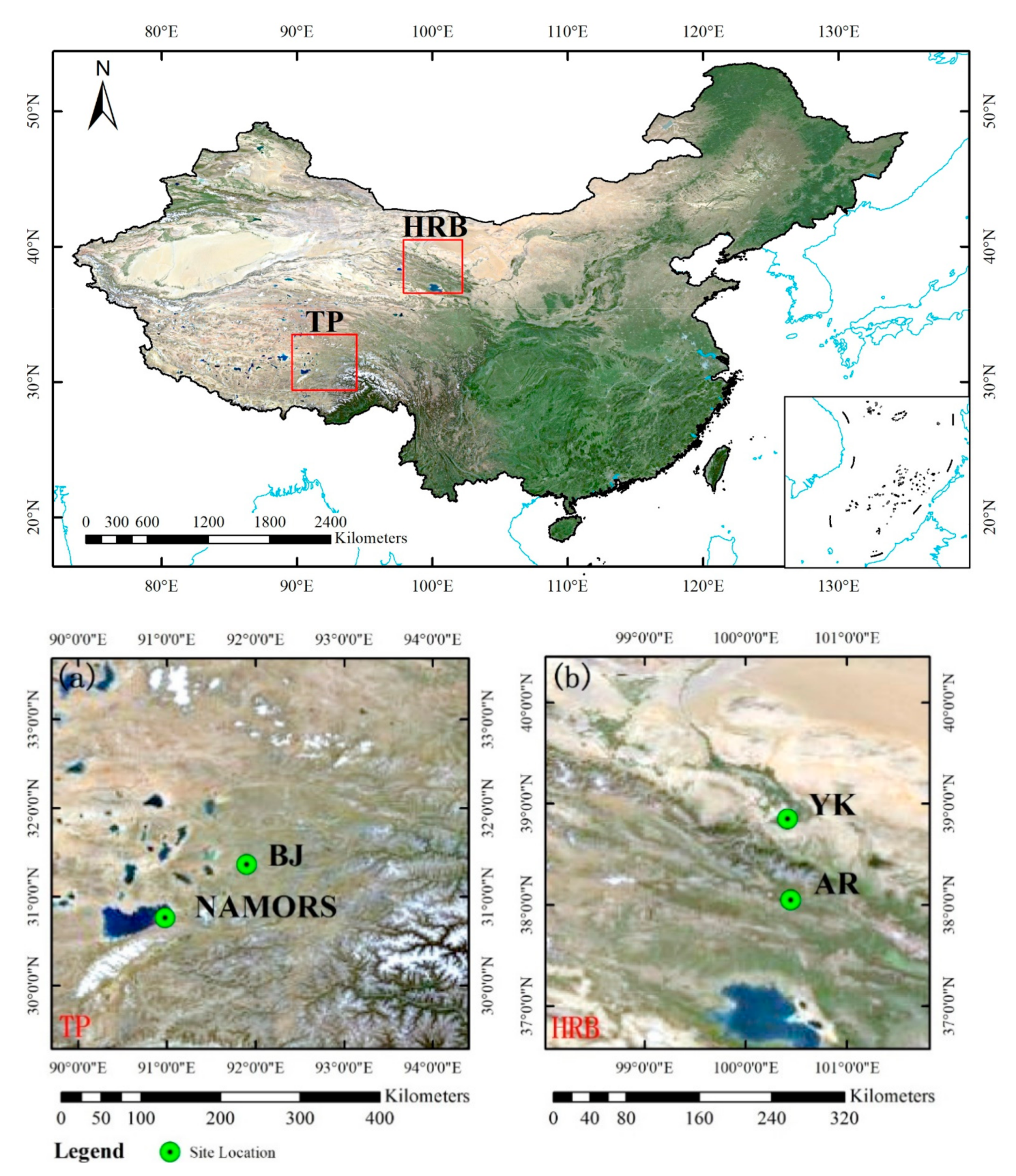
Frequent cloud coverage in China has limited the application of TIR LST in this region. Therefore, mainland China was chosen as the study area, and its location is shown in Figure 1. Its background is the true color image. The terrain of China is highly complex, and its ecosystems range from glaciers and deserts to grasslands, wetlands, tropical rain forests, lakes, and oceans, which leads to large spatial temperature differences within its territory [38]. Furthermore, its climate is mainly wet monsoon and dry seasons, which leads to drastic temperature changes between seasons [39].
Two verification regions were chosen in the Tibetan Plateau (TP) region and the Heihe River Basin (HRB) region, respectively. The verification region in the TP is located near the city of Naqu. The elevation range of this verification region ranges from 2752 m to 6994 m and the average slope is 5.26°. Its land cover (LC) is mainly savanna and grassland. The verification region in the HRB is located on the border of Qinghai Province and Gansu Province. Its surface elevation is 1056–5314 m. The average slope of the Qilian Mountains in the southwest and the plains in the northeast is 7.27° and 1.03°, respectively. Its LC types include cropland, forest, sparse grassland, and barren land. The locations of the TP and HRB regions are indicated by two red rectangles in Figure 1, and the locations of in situ measurement sites are marked in Figure 1a,b with green circle symbols.
2.2. Data
Daily AMSR-E brightness temperature (BT) and MODIS LST were used as the main data. To obtain the PMW LST data required for the RF fusion process, LC data, snow cover data, elevation data, desert distribution data, and normalized difference vegetation index (NDVI) data were required in the selected PMW LST generation method [40]. As LST is regulated by LC type, terrain, and vegetation, the data corresponding to these factors are needed during the RF fusion process [41]. In addition, longitude and latitude belong to spatial information and can reflect the moisture condition from coastal to inland areas, while latitude maps can reflect the difference in solar radiation [42]. The study by Hengl, et al. [43] proved that considering the latitude and longitude when using the ML algorithm can strengthen the spatial interaction in the training process of the trees and improve spatial nonstationarity. The downward shortwave radiation (DSR) represents the difference in solar radiation at different latitudes, so DSR data can also reflect the difference in spatial position to a certain extent. Therefore, the data used in the RF fusion process also included longitude, latitude, and DSR data. In addition, the in situ data from the HRB and TP regions were used as reference data to verify the accuracy of the selected model.
2.2.1. Satellite Data
AMSR-E is a microwave sensor on board an Aqua satellite. The AMSR-E BT data were obtained from the National Snow & Ice Data Center (NSIDC) (https://nsidc.org/) (Last accessed on 4 June 2021). The data included the BT data for six different frequencies (6.9, 10.7, 18.7, 23.8, 36.5, and 89.0 GHz) in two polarization channels (horizontal and vertical polarization).
MODIS is an important sensor onboard the Terra and Aqua satellites. The AMSR-E and MODIS sensors on the Aqua satellite observe the Earth’s surface simultaneously, at approximately 1:30 p.m. local time in the daytime and 1:30 a.m. local time at night. The MODIS data were provided by the Level-1 and Atmosphere Archive & Distribution System (LAADS) Distributed Active Archive Center (DAAC) (https://ladsweb.modaps.eosdis.nasa.gov/) (Last accessed on 4 June 2021), which contains MODIS LST products, LC products, snow products, and NDVI products. The MODIS LST product (MYD11A1) was derived from two MODIS thermal infrared channels (31 and 32) using the generalized split-window algorithm [44], which contains daily daytime and nighttime LST, quality control (QC), and transit time information. The QC information was used to identify high-quality MODIS LST pixels. LST pixels that were displayed as “LST produced”, “good data quality”, “average emissivity error ≤ 0.02”, and “average LST error ≤ 1 K” in the QC layer were considered high-quality pixels and used in this study. The transit time information for each pixel was used to match the pixel with the in situ data. In addition, the spatial information and latitude and longitude data can also be acquired from this LST dataset. The LC data generated according to the International Geosphere-Biosphere Programme (IGBP) classification system in the MODIS LC product (MCD12Q1) was used for this study. This LC type data were used for the PMW LST generation and RF fusion process. In the RF fusion process, LC type data were simply synthesized into 5 types, namely soil, vegetation, water, ice and snow, and buildings. The MODIS snow cover product (MYD10C1), which represents the percentage of snow area in the entire grid area, provides the snow data required by the PMW LST generation process. The NDVI data provided by the MODIS vegetation index product (MYD13A2) product were used in the PMW LST generation process, and also used in the RF fusion process as vegetation-related information.
The elevation data was the Shuttle Radar Topography Mission (SRTM) dataset, which is a global elevation dataset collected by the radar onboard the space shuttle Endeavour in February 2000. The data were downloaded from http://srtm.csi.cgiar.org/srtmdata/ (Last accessed on 4 June 2021). These elevation data and the slope data generated based on these elevation data were used for the PMW LST generation process.
The desert distribution data required during the PMW LST generation process were the China desert distribution vector data and were downloaded from the Cold and Arid Region Science Data Center (http://westdc.westgis.ac.cn) (Last accessed on 12 October 2018). The data needed to be converted into raster data for use [45].
The DSR data were obtained from the Global Land Surface Satellite (GLASS) products. The GLASS DSR products are generated from the data of multiple polar-orbit satellites (MODIS) and geostationary satellites (Geostationary Operational Environmental Satellite (GOES) imager; Meteosat Second Generation (MSG) SEVIRI; Multi-functional Transport Satellite (MTSAT)-1R imager) using an improved look-up table (LUT) method by radiative simulation based on MODTRAN [46,47]. The DSR data were downloaded from the National Earth System Science Data Center, National Science & Technology Infrastructure of China (http://www.geodata.cn) (Last accessed on 4 June 2021), and were used in the RF fusion process.
The basic information of the datasets used in this study is shown in Table 1. The study period ranges from 1 January 2010 to 31 December 2010. The MYD11A1, MCD12Q1, MYD10C1, MYD13A2, SRTM DEM, map of the desert distribution of China, and GLASS DSR were uniformly converted into geographical latitude/longitude coordinates and resampled to a spatial resolution of 0.01°.
2.2.2. In Situ Measurements
In order to evaluate the fused LST, a land–atmosphere interaction observations dataset from the TP region [48], and the Automatic Weather Stations dataset (AWS) from the Heihe region [49] were used.
The land–atmosphere interaction observations dataset was downloaded from the National Tibetan Plateau Data Center (https://0-doi-org.brum.beds.ac.uk/10.11888/Meteoro.tpdc.270910) (Last accessed on 4 June 2021) [48]. It includes the four-component radiation, multi-layer soil temperature, humidity and soil heat flux, and other observations. In this study, the data from the BJ site of Nagqu Station of Plateau Climate and Environment and Nam Co Monitoring and Research Station (NAMORS) for Multisphere Interactions were selected as the verification data. The LC types of BJ and NAMORS sites are alpine meadow and alpine steppe, respectively.
The AWS dataset was obtained from Watershed Allied Telemetry Experimental Research (WATER), which was provided by the Heihe Plan Data Management Center (http://www.heihedata.org/) (Last accessed on 12 October 2018) [49]. The observation items included the four-component radiation, the multi-layer soil temperature, soil moisture, soil heat flux, and other observation. The data from the Arou (AR) and Yingke (YK) sites were selected as the verification data in the study. The LC types of AR and YK sites are alpine meadow and cropland, respectively. The basic information about these verification sites is presented in Table 2. The locations of these sites are marked with green circle symbols in Figure 1a,b.
The radiation data, including the surface longwave upwelling and downward radiation, were used in the verification process to calculate in situ temperature data, and the temperature data were calculated by using the Stefan–Boltzmann law, as shown in the following equation:
In the equation, is the calculated in situ temperature data; and are the surface longwave upwelling radiation and the surface longwave downward radiation, respectively; is the Stefan–Boltzmann constant (); and is the surface broadband emissivity, which was computed from the ASTER GED product [50] by using the following equation according to Cheng, et al. [51]:
In the equation, – are the surface narrowband emissivity data of ASTER bands 10–14, respectively.
The time resolution of these radiation measurements in the TP and HRB regions was 1 h and 30 min, and the radiation measurements with the closest observation time to the transit time of MODIS were selected for the verification process. Therefore, the time difference between the field observation and satellite overpass in the TP region was no more than 30 min, and the time difference in the HRB region was less than 15 min.
3. Methodology
3.1. PMW LST Data Generation
In this study, the LUT-based AMSR-E LST retrieval algorithm proposed by Zhang and Cheng [40] was used to generate AMSR-E LST data. The main idea of this algorithm is to establish a comprehensive classification system of environmental variables (CCSEV). The data in the SRTM DEM, MCD12Q1, map of the desert distribution of China, and MYD10C1 datasets represent these factors for the establishment of the CCSEV. Then, the AMSR-E BT and the upscaled MODIS LST obtained by simple averaging were subjected to stepwise regression, and the retrieval formula for each CCSEV class was established separately. The accuracy (root mean square error (RMSE)) of the AMSR-E LST retrieved by this method was 2.65–3.48 K during the daytime and 2.15–2.94 K at nighttime. For the specific content of the LST retrieval algorithm, please refer to Zhang and Cheng [40].
The AMSR-E LST data were used in RF to achieve the fusion with the MODIS LST data. The AMSR-E LST data as PMW data represent the true situation of the cloudy-sky land surface. In order to obtain high spatial resolution all-weather LST, the AMSR-E LST data were downscaled to a spatial resolution consistent with the MODIS LST. A downscaling method based on the geographic weighted regression (GWR) model was used. This method sets a series of intermediate resolution levels between the initial resolution of 0.25° and the target resolution of 0.01°, and then uses the GWR model to establish the relationship between the LST and the scale conversion factor at each level in turn, and gradually downscales the AMSR-E LST from 0.25° to 0.01°. In this method, its scale conversion factor is usually NDVI data and elevation and slope data. Therefore, the NDVI data in MYD13A2, the elevation data in SRTM DEM, and the slope data generated by the elevation data were used. For more details on the GWR method, please see Zhang, et al. [52]. The downscaled AMSR-E LST data were generated by the above two methods.
3.2. LST Fusion Based on RF Method
LST is affected by many complex factors, so the selection of the best independent variable combination is crucial for LST fusion. Theoretically, the spatiotemporal pattern of LST is related to terrain, LC, soil moisture, and incoming solar radiation [41]. Therefore, in this study, elevation, NDVI, LC, longitude and latitude, and DSR were selected as candidate variables. The spatial distribution of LST is related to the topographical fluctuations in the study area, so elevation is a necessary predictor [53,54,55]. Since the vegetation-covered area accounts for 97.4% of the total area within the study area, which was calculated by LC data, NDVI data were also used as a necessary predictor to further describe the vegetation characteristics. Considering that the impact of LC on LST can be studied, LC was also selected as a candidate indicator [56].
RF, an integrated ML algorithm that evolved from the bagging algorithm, can be used for regression and classification research [34]. As a nonlinear method, RF consists of many decision trees. These decision trees are constructed from a randomly selected subset to lower the correlation between different decision trees [57,58]. The final output of the RF model is obtained by combining the results of all decision trees. The RF model has few parameter settings, fast training speed, high prediction accuracy, and can accurately capture the nonlinear interaction between variables [59]. In addition, the RF method is also an effective method to predict missing data, which can maintain accuracy even when most of the data are absent [60]. Thus, the RF method was chosen to accurately express the nonlinear relationship between LST and the important factors affecting it, and to achieve the purpose of using only clear-sky data to predict all-weather LST. However, because the input in the RF method is a series of values that does not contain spatial information, this method lacks the spatial information contained in the RS data. Longitude and latitude belong to spatial information and also reflect the difference of soil moisture and solar radiation, so its inclusion will likely improve the results of the fusion. DSR represents the differences in solar radiation at different latitudes, and it can also be used to characterize differences in spatial position.
Therefore, in this study, the candidate variables for the RF model include elevation, NDVI, LC, longitude and latitude, and DSR. Among them, elevation, NDVI, longitude and latitude, and DSR were directly used as independent variables, and LC was used to segregate data into different data bins. Four RF models composed of different candidate variables were tested, of which models ii-iv considered spatial information, as follows: (i) downscaled AMSR-E LST, elevation, and NDVI are the independent variables, clear-sky MODIS LST is the dependent variable; (ii) based on model i, latitude and longitude are added as independent variables; (iii) based on model ii, data are separated into different bins according to the LC type, and an RF model trained for each bin separately; (iv) based on model i, DSR is added as an independent variable, data are separated into different bins according to the LC type, and an RF model trained for each bin separately. Table 3 shows the variable selection status of the four candidate RF models. The RMSE was used as an indicator to select the best RF model among the four candidate models. The best selected RF model was used to achieve LST data fusion and thus predict all-weather LST data.
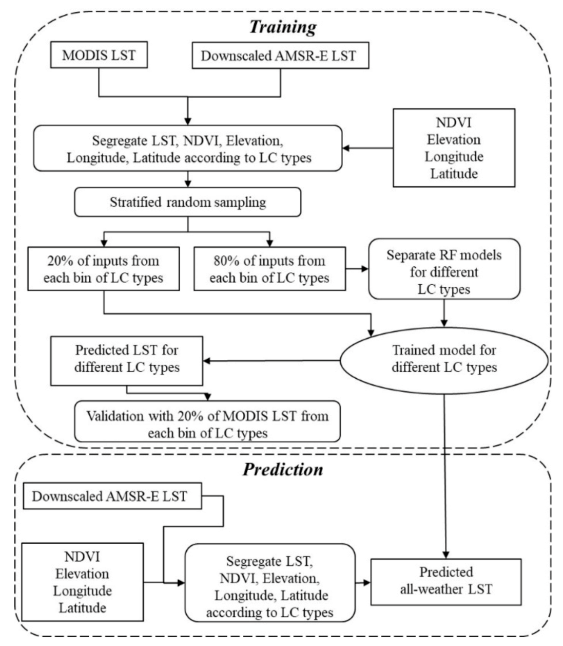
The most complicated model, model iii, was used as an example, and the flowchart for implementing model iii is shown in Figure 2. The process can be divided into training and prediction; before the training process begins, the input data were selected according to the availability of MODIS LST (using QC information as an indicator, see Section 2.2.1 for details). The steps in the training process were as follows:
- (1)
- Separate MODIS LST, downscaled AMSR-E LST, NDVI, elevation, and longitude and latitude data to different bins according to LC type in the MODIS LC data;
- (2)
- Use stratified random sampling to divide the input data of each bin into two parts: 80% of inputs from each bin were randomly selected as the training data, and the remaining 20% of inputs from each bin were reserved as verification data;
- (3)
- Train the RF model separately for each LC type;
- (4)
- Use the corresponding RF model to predict LST of each LC type separately in the remaining 20% of inputs;
- (5)
- Calculate the RMSE value of the predicted LST and the remaining MODIS LST, which was used to select the best RF model.
The steps of the prediction process are as follows:
- (1)
- Separate the downscaled AMSR-E LST, NDVI, elevation, and longitude and latitude data into different bins according to different LC type;
- (2)
- Use the RF model obtained from the training process to predict all-weather LST. See Section 4.1 for the selection results of the best RF model.
4. Results
4.1. Comparison of RF Model Results
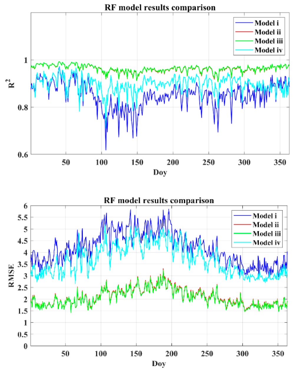
Four RF models were used to fuse the daytime LST data for the year 2010. Figure 3 shows the training results of the RF models. The values of the four RF models were between 0.6 and 1, while the values of models ii and iii were both close to 1. The RMSE of the four RF models was between 1.5 K and 6 K, among which the RMSEs of models ii and iii were relatively low (between 1.5 K and 3 K), and the RMSEs of models i and iv were relatively high (between 2.5 K and 6 K). Model i, which did not consider spatial information, had the worst effect, including the lowest value and the highest RMSE. Models ii and iii, containing longitude and latitude information, performed relatively well. Compared to model ii, model iii performed best because it not only considered the effects of NDVI, elevation, and latitude and longitude, but also modeled different models for the data corresponding to different LC types. This may be because the temperature generation mechanism varies with the LC type, and thus modeling each LC type separately will slightly improve the accuracy of the fusion result. Since the DSR data in model iv can only represent changes in latitude, their accuracy is lower than that of model iii. Therefore, model iii was selected as the final model to fuse the MODIS and AMSR-E LST data.
4.2. The Effect of the Fused LST
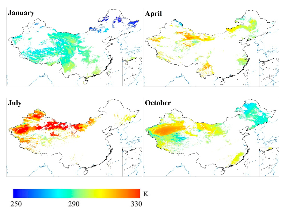
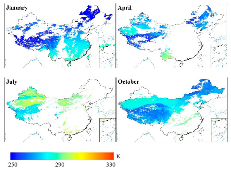
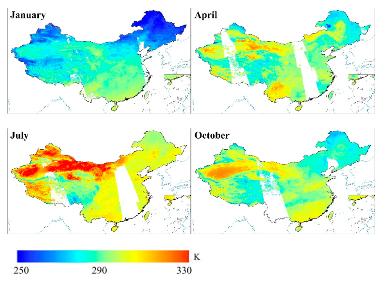
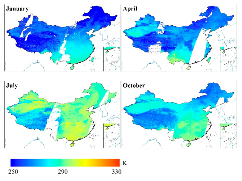
The effect of the fused LST was investigated from two aspects: qualitative analysis and quantitative verification. We adopted days of the year to represent the twelve months for MODIS LST. Spatial patterns of MODIS LST during daytime and nighttime are shown in Figure 4 and Figure 5, respectively. Severe data loss was observed on each day due to the impact of cloud contamination. Figure 6 and Figure 7 show the spatial patterns of the fusion results corresponding to these MODIS LST data. Compared with MODIS LST, the spatial integrity of the fusion results was greatly improved, except for some blank areas caused by the orbit gap of the AMSR-E sensor. In addition, in terms of time, the magnitude of LST data in these images gradually increases from January to July, and gradually decreases from August to December. In space, the LST in northeast China and the Qinghai–Tibet Plateau is relatively low, while the LST in south China and the desert areas in northwest China is relatively high. This indicates that the magnitude of LST data in the fusion results is consistent with the general spatiotemporal variations of LST.
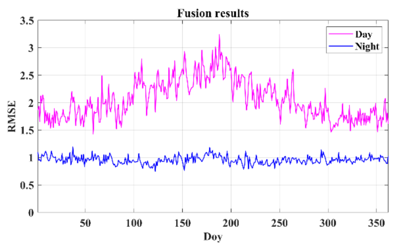
Lastly, we tested the fused LST using the reserved 20% MODIS LST data (Figure 8). We found that the nighttime RMSE was smaller than the daytime RMSE, with the daytime RMSE around 2 K, and the nighttime RMSE around 1 K.
4.3. Verification Using In Situ Measurements
4.3.1. LST Verification
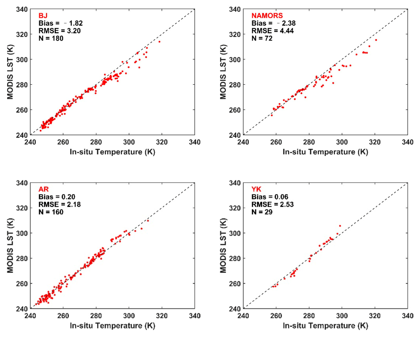
The in situ temperature data calculated by the surface longwave upwelling and downward radiation were used in the verification process. For comparison, both MODIS LST data and fused LST were verified. Figure 9 shows the scatter plots of the in situ temperature and MODIS LST. The RMSE of MODIS LST was 3.20 K, 4.44 K, 2.18 K, and 2.53 K at the BJ, NAMORS, AR, and YK stations, respectively.
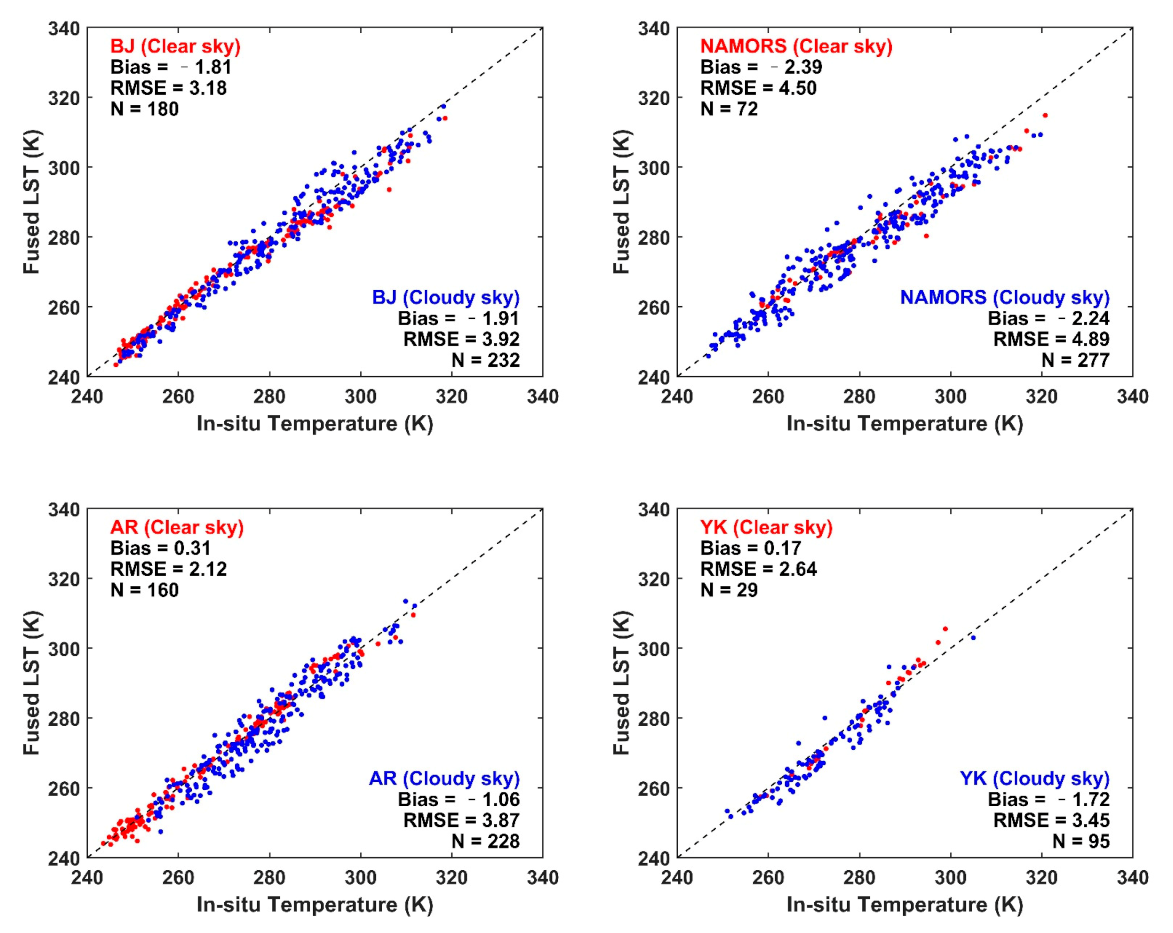
The scatter plots of the in situ temperature and fused LST are provided in Figure 10. At the BJ, NAMORS, AR, and YK stations, the RMSE of clear-sky fused LST was 3.18 K, 4.50 K, 2.12 K, and 2.64 K, which was similar to the RMSE of MODIS LST, indicating similar accuracy of the clear-sky fused LST and MODIS LST. The RMSE of cloudy-sky fused LST was 3.92 K, 4.89 K, 3.87 K, and 3.45 K, respectively. The accuracy of cloudy-sky fused LST was lower than that of clear-sky fused LST. This is because the accuracy of PMW LST is relatively low under conditions of cloud coverage [20]. However, these cloudy-sky RMSE values can be compared with the cloudy-sky RMSE values of previous machine learning methods. A neural network retrieval method proposed by Aires, et al. [61] has an RMSE value of about 3.1–5 K under cloudy conditions in mid-latitude regions [62]. The machine learning method based on artificial neural network (ANN) models used by Shwetha and Kumar [23] has RMSE values of 2.9–6.2 K for cloudy sky during daytime, and 2.1–3.3 K for cloudy sky during nighttime. In addition, the bias indicates that the cloudy-sky fused LST at all sites was lower than the in situ temperature, which may be related to the slightly deeper thermal sampling depth of the PMW radiation during PMW data collection [14].
4.3.2. The Daily Variation of the Fusion LST
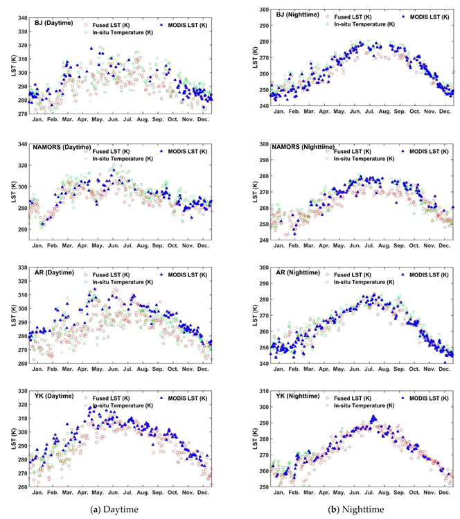
The daily variation of fused LST at all sites during 2010 is shown in Figure 11. For reference, the daily variations of the in situ temperature and MODIS LST are also included in this figure. In each figure, the trend of the fused LST time series is close to the trend of the in situ temperature time series and MODIS LST time series, and is consistent with the correct annual LST trend. Therefore, it can be concluded that the LST fused by the RF method can capture the correct time variation of the LST at each site. The deviation of the daytime fused LST is relatively large, which can also be explained by the slightly deeper thermal sampling depth of PMW radiation [14].
5. Discussion
5.1. Improvement of Integrity
As shown in Figure 6 and Figure 7, due to the orbital gap of the AMSR-E sensor, the fused LSTs still have missing values. To further improve the effectiveness of the fusion results, the data interpolating empirical orthogonal function (DINEOF) method was used. The DINEOF method was proposed by Beckers and Rixen in 2003 and is often used to deal with the problem of missing data [63]. Compared with traditional interpolation methods, the DINEOF method requires fewer input parameters and has higher computational efficiency [64]. This method has been used in many studies and reliable results have been obtained with it [64,65,66,67,68,69,70,71].
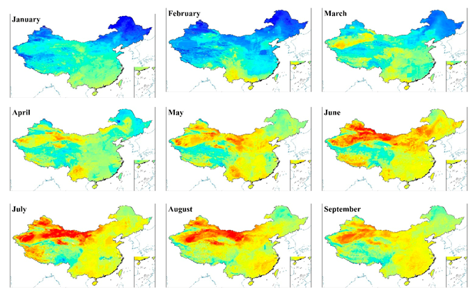
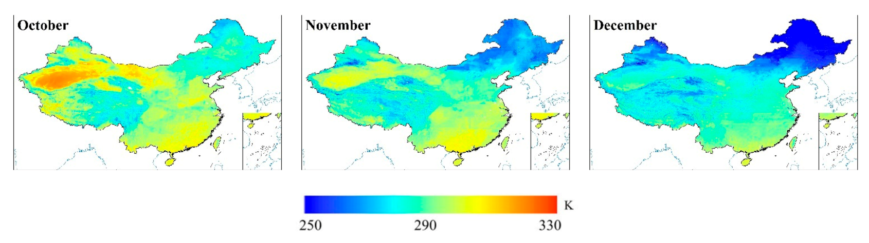
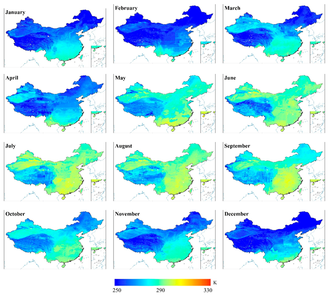
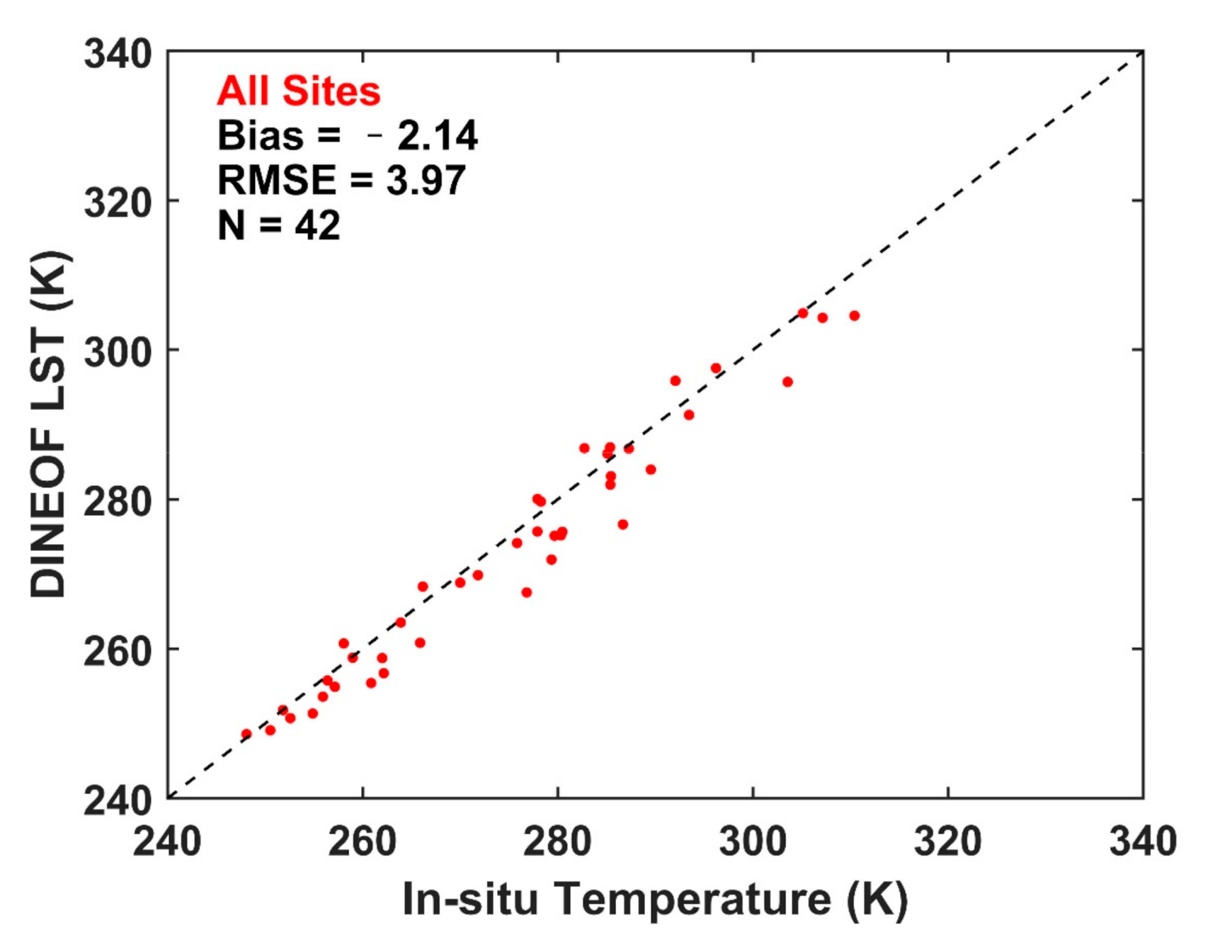
Figure 12 and Figure 13 show the spatial distributions of the complete all-weather LST in different months, indicating that the DINEOF method effectively improves the integrity of the fusion result. In addition, in order to further evaluate the performance of the DINEOF method for filling LST values in the satellite orbit gap, the in situ temperature data were used to verify these complete all-weather LST data, shown in Figure 12 and Figure 13. The scatter plot of the in situ temperature and the all-weather LST data is shown in Figure 14. The RMSE of all-weather LST was 3.97 K, which was similar to the average RMSE of the fused LST (3.57 K), indicating that by combining the RF fusion method and the DINEOF method, the complete all-weather LST with high spatial resolution can be generated.
5.2. Factors Affecting the Fusion Results
5.2.1. Effects of Missing Value Proportion
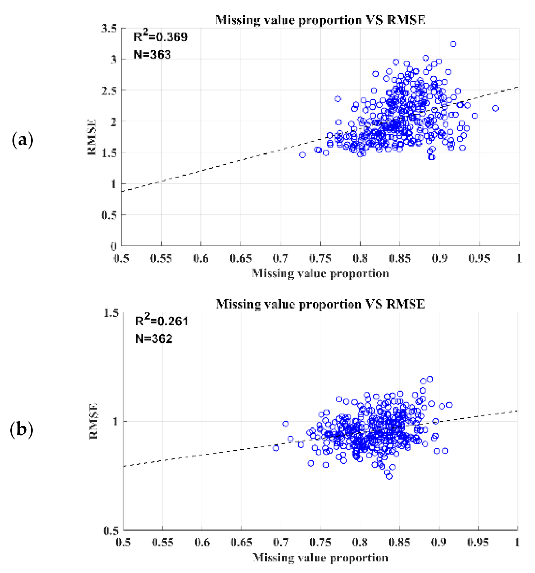
It can be seen from Figure 8 that the RMSE of the fusion results varies with the date, which may be related to the missing value proportions. Figure 15 shows the scatter plot of missing value proportions and RMSE, and highlights that RMSE has a positive relationship with the missing value proportions. For dates with a large missing value proportion, the accuracy of the fusion result was generally low, and vice versa.
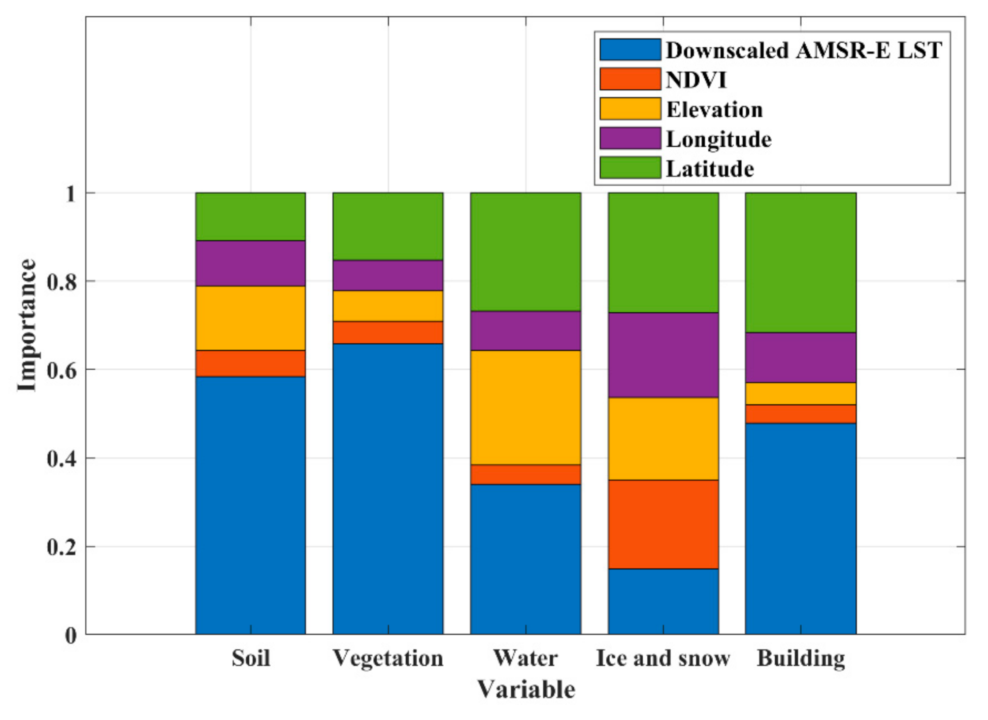
5.2.2. Variable Importance Measure
To investigate the contribution of the input variables in the selected models to the fusion results, the variable importance measures provided by the RT method were used. As shown in Figure 16, downscaled AMSR-E LST and latitude had a significant effect on the LST estimates, while NDVI and elevation had the least effect on the LST estimates, except for snow and ice, as well as the water LC type. This can be attributed to the contribution already made by NDVI and elevation data during the PMW LST downscaling process.
5.3. Accuracy Comparison with Downscaled AMSR-E LST
Methods for obtaining complete high-resolution LST can be divided into two categories: kernel-driven methods, which downscale LST through auxiliary data to obtain high-resolution LST; and fusion-based methods, which predict all-weather high-resolution LST by integrating information from different sensors [72]. In this study, the downscaled AMSR-E LST was a high-resolution LST obtained by the kernel-driven method; the fused LST is an all-weather high-resolution LST predicted by the fusion-based method.
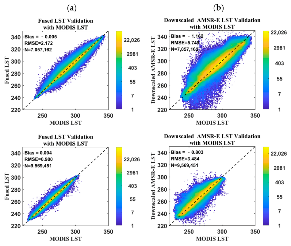
In order to explore the necessity of the RF fusion process, MODIS LST was used as verification data to verify the fusion results and the downscaled AMSR-E LST. Figure 17a,b are the scatter density plots of the fusion results and the downscaled AMSR-E LST, respectively, where the first row is daytime data and the second row is nighttime data. It can be seen from Figure 17 that the scatter points of the fusion results are closely distributed around the 1:1 line, whereas the downscaled AMSR-E LSTs are more scattered during both the daytime and nighttime. In addition, the RMSE was obtained and compared to the reserved 20% MODIS LST. The RMSE of the daytime and nighttime LST data obtained by directly downscaling the PMW LST was 5.75 K and 3.48 K, respectively. The RMSE of the daytime and nighttime LST obtained by fusing the TIR and PMW LST data was significantly reduced by 62.21% and 71.87%, respectively, and its RMSE was 2.17 K and 0.98 K. Therefore, in order to obtain more accurate all-weather high-resolution LST, the process of fusing TIR and PMW LST data with the RF method is necessary.
6. Conclusions
In this study, the RF model was used to fuse MODIS and AMSR-E LST in mainland China during 2010. The RF model performed best when LC type, terrain, vegetation conditions, moisture conditions, and solar radiation were considered. The magnitude of LST data in the fusion result is consistent with the general spatiotemporal variation of LST.
In order to further evaluate the effectiveness of the RF model, the in situ measurements obtained from the central TP region and upper and middle reaches of the HRB region were used to verify the fused LST. The RMSE of clear-sky fused LST and cloudy-sky fused LST were 2.12–4.50 K and 3.45–4.89 K, respectively. According to the fused LST images of China on the 15th day of each month in 2010 and the time series of fused LST at the verification sites, we found that the fused results of the RF model accurately reflected the spatiotemporal change trend of LST. To further improve the usability of the all-weather LST, the DINEOF method was used to obtain a complete all-weather LST. By exploring the relationship between the RMSE and the missing value proportions, we found that high RMSEs usually corresponded to a large missing value proportion and vice versa. With reference to the variable importance measures, it can be seen that the downscaled AMSR-E LST and latitude have the most significant impact on LST estimation. Compared with the high-resolution LST obtained through downscaling of AMSR-E data, the fusion method of estimating LST had higher accuracy, indicating that it is necessary to use the RF fusion method. The proposed method effectively fuses TIR and PMW LST data, thereby generating all-weather LST data with high spatial resolution.
Author Contributions
Conceptualization, S.X. and J.C.; Data curation, S.X.; Funding acquisition, J.C.; Investigation, S.X.; Methodology, S.X. and Q.Z.; Writing—Original draft, S.X.; Writing—Review and editing, J.C. All authors have read and agreed to the published version of the manuscript.
Funding
This work was supported in part by the National Key Research and Development Program of China under Grant 2016YFA0600101, in part by the National Natural Science Foundation of China under Grant 42071308 and Grant 41771365, and in part by the Open Funding of Beijing Municipal Engineering and Technology Center for Land Surface Remote Sensing Data Products.
Conflicts of Interest
The authors declare that they have no known competing financial interest or personal relationships that could have appeared to influence the work reported in this paper.
References
- Anderson, M.; Norman, J.; Kustas, W.; Houborg, R.; Starks, P.; Agam, N. A thermal-based remote sensing technique for routine mapping of land-surface carbon, water and energy fluxes from field to regional scales. Remote Sens. Environ. 2008, 112, 4227–4241. [Google Scholar] [CrossRef]
- Li, Z.; Tang, R.; Wan, Z.; Bi, Y.; Zhou, C.; Tang, B.; Yan, G.; Zhang, X. A review of current methodologies for regional evapotranspiration estimation from remotely sensed data. Sensors 2009, 9, 3801–3853. [Google Scholar] [CrossRef] [PubMed] [Green Version]
- Zhou, J.; Chen, Y.; Wang, J.; Zhan, W. Maximum nighttime urban heat island (UHI) intensity simulation by integrating remotely sensed data and meteorological observations. IEEE J. Sel. Top. Appl. Earth Obs. Remote Sens. 2011, 4, 138–146. [Google Scholar] [CrossRef]
- Kalma, J.D.; McVicar, T.R.; McCabe, M.F. Estimating land surface evaporation: A review of methods using remotely sensed surface temperature data. Surv. Geophys. 2008, 29, 421–469. [Google Scholar] [CrossRef]
- Li, Z.-L.; Tang, B.-H.; Wu, H.; Ren, H.; Yan, G.; Wan, Z.; Trigo, I.F.; Sobrino, J.A. Satellite-derived land surface temperature: Current status and perspectives. Remote Sens. Environ. 2013, 131, 14–37. [Google Scholar] [CrossRef] [Green Version]
- Cheng, J.; Liang, S.; Meng, X.; Quan, Z.; Zhou, S. Chapter 7—Land surface temperature and thermal infrared emissivity. In Advanced Remote Sensing, 2nd ed.; Liang, S., Wang, J., Eds.; Academic Press: Cambridge, MA, USA, 2020; pp. 251–295. [Google Scholar]
- Liang, S. Advanced Remote Sensing; Academic Press: Cambridge, MA, USA, 2012. [Google Scholar]
- Cornette, W.M.; Shanks, J.G. Impact of cirrus clouds on remote sensing of surface temperatures. In Proceedings of the Passive Infrared Remote Sensing of Clouds and the Atmosphere, Orlando, FL, USA, 11–16 April 1993; pp. 252–264. [Google Scholar]
- Wan, Z. New refinements and validation of the MODIS Land-Surface Temperature/Emissivity products. Remote Sens. Environ. 2008, 112, 59–74. [Google Scholar] [CrossRef]
- Duan, S.-B.; Li, Z.-L.; Li, H.; Göttsche, F.-M.; Wu, H.; Zhao, W.; Leng, P.; Zhang, X.; Coll, C. Validation of Collection 6 MODIS land surface temperature product using in situ measurements. Remote Sens. Environ. 2019, 225, 16–29. [Google Scholar] [CrossRef] [Green Version]
- Duan, S.-B.; Li, Z.-L.; Wu, H.; Leng, P.; Gao, M.; Wang, C. Radiance-based validation of land surface temperature products derived from Collection 6 MODIS thermal infrared data. Int. J. Appl. Earth Obs. Geoinf. 2018, 70, 84–92. [Google Scholar] [CrossRef]
- Wang, K.; Liang, S. Evaluation of ASTER and MODIS land surface temperature and emissivity products using long-term surface longwave radiation observations at SURFRAD sites. Remote Sens. Environ. 2009, 113, 1556–1565. [Google Scholar] [CrossRef]
- Liu, Y.; Yu, Y.; Yu, P.; Göttsche, F.; Trigo, I. Quality Assessment of S-NPP VIIRS Land Surface Temperature Product. Remote Sens. 2015, 7, 12215. [Google Scholar] [CrossRef] [Green Version]
- Zhou, J.; Dai, F.; Zhang, X.; Zhao, S.; Li, M. Developing a temporally land cover-based look-up table (TL-LUT) method for estimating land surface temperature based on AMSR-E data over the Chinese landmass. Int. J. Appl. Earth Obs. Geoinf. 2015, 34, 35–50. [Google Scholar] [CrossRef]
- McFarland, M.J.; Miller, R.L.; Neale, C.M. Land surface temperature derived from the SSM/I passive microwave brightness temperatures. IEEE Trans. Geosci. Remote Sens. 1990, 28, 839–845. [Google Scholar] [CrossRef]
- Calvet, J.; Wigneron, J.; Mougin, E.; Kerr, Y.H.; Brito, J.L.S. Plant water content and temperature of the Amazon forest from satellite microwave radiometry. IEEE Trans. Geosci. Remote Sens. 1994, 32, 397–408. [Google Scholar] [CrossRef]
- Liang, S.; Wang, D.; Tao, X.; Cheng, J.; Yao, Y.; Zhang, X.; He, T. 2.12—Methodologies for Integrating Multiple High-Level Remotely Sensed Land Products. In Comprehensive Remote Sensing; Liang, S., Ed.; Elsevier: Oxford, UK, 2018; pp. 278–317. [Google Scholar] [CrossRef]
- Wu, P.; Yin, Z.; Zeng, C.; Duan, S.; Gottsche, F.-M.; Ma, X.; Li, X.; Yang, H.; Shen, H. Spatially Continuous and High-resolution Land Surface Temperature: A Review of Reconstruction and Spatiotemporal Fusion Techniques. arXiv 2019, arXiv:1909.09316. [Google Scholar]
- Wang, T.; Shi, J.; Yan, G.; Zhao, T.; Ji, D.; Xiong, C. Recovering land surface temperature under cloudy skies for potentially deriving surface emitted longwave radiation by fusing MODIS and AMSR-E measurements. In Proceedings of the 2014 IEEE Geoscience and Remote Sensing Symposium, Quebec City, QC, Canada, 13–18 July 2014; pp. 1805–1808. [Google Scholar]
- Duan, S.-B.; Li, Z.-L.; Leng, P. A framework for the retrieval of all-weather land surface temperature at a high spatial resolution from polar-orbiting thermal infrared and passive microwave data. Remote Sens. Environ. 2017, 195, 107–117. [Google Scholar] [CrossRef]
- Zhang, X.; Zhou, J.; Gottsche, F.M.; Zhan, W.; Liu, S.; Cao, R. A Method Based on Temporal Component Decomposition for Estimating 1-km All-Weather Land Surface Temperature by Merging Satellite Thermal Infrared and Passive Microwave Observations. IEEE Trans. Geosci. Remote Sens. 2019, 57, 4670–4691. [Google Scholar] [CrossRef]
- Xu, S.; Cheng, J.; Zhang, Q. Reconstructing All-Weather Land Surface Temperature Using the Bayesian Maximum Entropy Method Over the Tibetan Plateau and Heihe River Basin. IEEE J. Sel. Top. Appl. Earth Obs. Remote Sens. 2019, 12, 3307–3316. [Google Scholar] [CrossRef]
- Shwetha, H.; Kumar, D.N. Prediction of high spatio-temporal resolution land surface temperature under cloudy conditions using microwave vegetation index and ANN. ISPRS J. Photogramm. Remote Sens. 2016, 117, 40–55. [Google Scholar] [CrossRef]
- Xu, S.; Cheng, J. A new land surface temperature fusion strategy based on cumulative distribution function matching and multiresolution Kalman fltering. Remote Sens. Environ. 2020, 254, 112256. [Google Scholar] [CrossRef]
- Sun, D.; Li, Y.; Zhan, X.; Houser, P.; Yang, R. Land Surface Temperature Derivation under All Sky Conditions through Integrating AMSR-E/AMSR-2 and MODIS/GOES Observations. Remote Sens. 2019, 11, 1704. [Google Scholar] [CrossRef] [Green Version]
- Long, D.; Yan, L.; Bai, L.; Zhang, C.; Shi, C. Generation of MODIS-like land surface temperatures under all-weather conditions based on a data fusion approach. Remote Sens. Environ. 2020, 246, 111863. [Google Scholar] [CrossRef]
- Zhang, X.; Zhou, J.; Liang, S.; Chai, L.; Wang, D.; Liu, J. Estimation of 1-km all-weather remotely sensed land surface temperature based on reconstructed spatial-seamless satellite passive microwave brightness temperature and thermal infrared data. ISPRS J. Photogramm. Remote Sens. 2020, 167, 321–344. [Google Scholar] [CrossRef]
- Martins, J.P.A.; Trigo, I.F.; Ghilain, N.; Jimenez, C.; Göttsche, F.-M.; Ermida, S.L.; Olesen, F.-S.; Gellens-Meulenberghs, F.; Arboleda, A. An All-Weather Land Surface Temperature Product Based on MSG/SEVIRI Observations. Remote. Sens. 2019, 11, 3044. [Google Scholar] [CrossRef] [Green Version]
- Stevens, F.R.; Gaughan, A.E.; Linard, C.; Tatem, A.J. Disaggregating Census Data for Population Mapping Using Random Forests with Remotely-Sensed and Ancillary Data. PLoS ONE 2015, 10, e0107042. [Google Scholar] [CrossRef] [Green Version]
- Song, H.; Liu, Q.; Wang, G.; Hang, R.; Huang, B. Spatiotemporal Satellite Image Fusion Using Deep Convolutional Neural Networks. IEEE J. Sel. Top. Appl. Earth Obs. Remote Sens. 2018, 11, 821–829. [Google Scholar] [CrossRef]
- Tan, Z.; Yue, P.; Di, L.; Tang, J. Deriving High Spatiotemporal Remote Sensing Images Using Deep Convolutional Network. Remote Sens. 2018, 10, 1066. [Google Scholar] [CrossRef] [Green Version]
- Liu, X.; Deng, C.; Chanussot, J.; Hong, D.; Zhao, B. StfNet: A Two-Stream Convolutional Neural Network for Spatiotemporal Image Fusion. IEEE Trans. Geosci. Remote Sens. 2019, 57, 6552–6564. [Google Scholar] [CrossRef]
- Yuan, Q.; Shen, H.; Li, T.; Li, Z.; Li, S.; Jiang, Y.; Xu, H.; Tan, W.; Yang, Q.; Wang, J. Deep learning in environmental remote sensing: Achievements and challenges. Remote Sens. Environ. 2020, 241, 111716. [Google Scholar] [CrossRef]
- Breiman, L. Random forests. Mach. Learn. 2001, 45, 5–32. [Google Scholar] [CrossRef] [Green Version]
- Georganos, S.; Grippa, T.; Gadiaga, A.N.; Linard, C.; Lennert, M.; Vanhuysse, S.; Mboga, N.; Wolff, E.; Kalogirou, S. Geographical random forests: A spatial extension of the random forest algorithm to address spatial heterogeneity in remote sensing and population modelling. Geocarto Int. 2019. [Google Scholar] [CrossRef] [Green Version]
- Foody, G.M. Geographical weighting as a further refinement to regression modelling: An example focused on the NDVI–rainfall relationship. Remote Sens. Environ. 2003, 88, 283–293. [Google Scholar] [CrossRef]
- Georganos, S.; Abdi, A.M.; Tenenbaum, D.E.; Kalogirou, S. Examining the NDVI-rainfall relationship in the semi-arid Sahel using geographically weighted regression. J. Arid. Environ. 2017, 146, 64–74. [Google Scholar] [CrossRef]
- Liu, J.; Diamond, J. China’s environment in a globalizing world. Nature 2005, 435, 1179–1186. [Google Scholar] [CrossRef]
- Fu, C.; Jiang, Z.; Guan, Z.; He, J.; Xu, Z. (Eds.) Climate Extremes and Related Disasters in China. In Climate Studies of China. Regional Climate Studies; Springer: Berlin/Heidelberg, Germany, 2008. [Google Scholar] [CrossRef]
- Zhang, Q.; Cheng, J. An Empirical Algorithm for Retrieving Land Surface Temperature From AMSR-E Data Considering the Comprehensive Effects of Environmental Variables. Earth Space Sci. 2020, 7, e2019EA001006. [Google Scholar] [CrossRef] [Green Version]
- Hengl, T.; Heuvelink, G.B.M.; Perčec Tadić, M.; Pebesma, E.J. Spatio-temporal prediction of daily temperatures using time-series of MODIS LST images. Theor. Appl. Climatol. 2012, 107, 265–277. [Google Scholar] [CrossRef] [Green Version]
- Duan, S.; Li, Z. Spatial Downscaling of MODIS Land Surface Temperatures Using Geographically Weighted Regression: Case Study in Northern China. IEEE Trans. Geosci. Remote Sens. 2016, 54, 6458–6469. [Google Scholar] [CrossRef]
- Hengl, T.; Nussbaum, M.; Wright, M.N.; Heuvelink, G.B.; Gräler, B. Random forest as a generic framework for predictive modeling of spatial and spatio-temporal variables. PeerJ 2018, 6, e5518. [Google Scholar] [CrossRef] [Green Version]
- Wan, Z.; Dozier, J. A generalized split-window algorithm for retrieving land-surface temperature from space. IEEE Trans. Geosci. Remote Sens. 1996, 34, 892–905. [Google Scholar]
- Wang, Y.M.; Wang, J.H.; Qi, Y.; Yan, C.Z. The map of desert distribution in 1:2,000,000 in China. Cold Arid. Reg. Sci. Data Cent. Lanzhou 1974. [Google Scholar] [CrossRef]
- Zhao, X. Generating Global LAnd Surface Satellite incident shortwave radiation and photosynthetically active radiation products from multiple satellite data. Remote Sens. Environ. 2014, 152, 318–332. [Google Scholar]
- Zhang, X.; Liang, S.; Song, Z.; Niu, H.; Wang, G.; Tang, W.; Chen, Z.; Jiang, B. Local Adaptive Calibration of the Satellite-Derived Surface Incident Shortwave Radiation Product Using Smoothing Spline. IEEE Trans. Geosci. Remote Sens. 2016, 54, 1156–1169. [Google Scholar] [CrossRef]
- Ma, Y.; Hu, Z.; Xie, Z.; Ma, W.; Wang, B.; Chen, X.; Li, M.; Zhong, L.; Sun, F.; Gu, L.; et al. A long-term (2005–2016) dataset of hourly integrated land–atmosphere interaction observations on the Tibetan Plateau. Earth Syst. Sci. Data 2020, 12, 2937–2957. [Google Scholar] [CrossRef]
- Li, X.; Li, X.; Li, Z.; Ma, M.; Wang, J.; Xiao, Q.; Liu, Q.; Che, T.; Chen, E.; Yan, G. Watershed allied telemetry experimental research. J. Geophys. Res. Atmos. 2009, 114. [Google Scholar] [CrossRef] [Green Version]
- Hulley, G.C.; Hook, S.J. The North American ASTER Land Surface Emissivity Database (NAALSED) Version 2.0. Remote Sens. Environ. 2009, 113, 1967–1975. [Google Scholar] [CrossRef]
- Cheng, J.; Liang, S.; Yao, Y.; Zhang, X. Estimating the Optimal Broadband Emissivity Spectral Range for Calculating Surface Longwave Net Radiation. IEEE Geosci. Remote Sens. Lett. 2013, 10, 401–405. [Google Scholar] [CrossRef]
- Zhang, Q.; Wang, N.; Cheng, J.; Xu, S. A Stepwise Downscaling Method for Generating High-Resolution Land Surface Temperature from AMSR-E Data. IEEE J. Sel. Top. Appl. Earth Obs. Remote Sens. 2020, 13, 5669–5681. [Google Scholar] [CrossRef]
- You, Q.; Kang, S.; Pepin, N.; Flügel, W.-A.; Yan, Y.; Behrawan, H.; Huang, J. Relationship between temperature trend magnitude, elevation and mean temperature in the Tibetan Plateau from homogenized surface stations and reanalysis data. Glob. Planet. Chang. 2010, 71, 124–133. [Google Scholar] [CrossRef]
- Chen, A.-A.; Wang, N.-L.; Guo, Z.-M.; Wu, Y.-W.; Wu, H.-B. Glacier variations and rising temperature in the Mt. Kenya since the Last Glacial Maximum. J. Mt. Sci. 2018, 15, 1268–1282. [Google Scholar] [CrossRef]
- Hutengs, C.; Vohland, M. Downscaling land surface temperatures at regional scales with random forest regression. Remote Sens. Environ. 2016, 178, 127–141. [Google Scholar] [CrossRef]
- Li, W.; Wu, H.; Duan, S.; Li, Z.; Liu, Q. Selection of Predictor Variables in Downscaling Land Surface Temperature using Random Forest Algorithm. In Proceedings of the IGARSS 2019—2019 IEEE International Geoscience and Remote Sensing Symposium, Yokohama, Japan, 28 July–2 August 2019; pp. 1817–1820. [Google Scholar]
- Hastie, T.; Tibshirani, R.; Friedman, J.H. The elements of statistical learning: Data mining, inference, and prediction. Math. Intell. 2005, 27, 83–85. [Google Scholar]
- Booksx, I. The fundamentals of risk measurement. Math. Intell. 2005, 27, 83. [Google Scholar]
- Belgiu, M.; Drăguţ, L. Random forest in remote sensing: A review of applications and future directions. Isprs J. Photogramm. Remote Sens. 2016, 114, 24–31. [Google Scholar] [CrossRef]
- Li, S.; Yuan, Q.; Yue, L.; Li, T.; Shen, H.; Zhang, L. Downscaling GNSS-R Based Vegetation Water Content Product Using Random Forest Model. In Proceedings of the IGARSS 2019—2019 IEEE International Geoscience and Remote Sensing Symposium, Yokohama, Japan, 28 July–2 August 2019; pp. 6720–6723. [Google Scholar]
- Aires, F.; Prigent, C.; Rossow, W.B.; Rothstein, M. A new neural network approach including first guess for retrieval of atmospheric water vapor, cloud liquid water path, surface temperature, and emissivities over land from satellite microwave observations. J. Geophys. Res. Atmos. 2001, 106, 14887–14907. [Google Scholar] [CrossRef]
- Catherinot, J.; Prigent, C.; Maurer, R.; Papa, F.; Jiménez, C.; Aires, F.; Rossow, W.B. Evaluation of “all weather” microwave-derived land surface temperatures with in situ CEOP measurements. J. Geophys. Res. Atmos. 2011, 116. [Google Scholar] [CrossRef] [Green Version]
- Beckers, J.; Rixen, M. EOF Calculations and Data Filling from Incomplete Oceanographic Datasets. J. Atmos. Ocean. Technol. 2003, 20, 1839–1856. [Google Scholar] [CrossRef]
- Zhou, W.; Peng, B.; Shi, J.; Wang, T.; Dhital, Y.P.; Yao, R.; Yu, Y.; Lei, Z.; Zhao, R. Estimating High Resolution Daily Air Temperature Based on Remote Sensing Products and Climate Reanalysis Datasets over Glacierized Basins: A Case Study in the Langtang Valley, Nepal. Remote Sens. 2017, 9, 959. [Google Scholar] [CrossRef] [Green Version]
- Alveraazcarate, A.; Barth, A.; Rixen, M.; Beckers, J. Reconstruction of incomplete oceanographic data sets using empirical orthogonal functions: Application to the Adriatic Sea surface temperature. Ocean. Model. 2005, 9, 325–346. [Google Scholar] [CrossRef] [Green Version]
- Alveraazcarate, A.; Barth, A.; Beckers, J.; Weisberg, R.H. Multivariate reconstruction of missing data in sea surface temperature, chlorophyll, and wind satellite fields. J. Geophys. Res. 2007, 112. [Google Scholar] [CrossRef] [Green Version]
- Miles, T.; He, R. Temporal and spatial variability of Chl-a and SST on the South Atlantic Bight: Revisiting with cloud-free reconstructions of MODIS satellite imagery. Cont. Shelf Res. 2010, 30, 1951–1962. [Google Scholar] [CrossRef]
- Nechad, B.; Alveraazcarate, A.; Ruddick, K.; Greenwood, N. Reconstruction of MODIS total suspended matter time series maps by DINEOF and validation with autonomous platform data. Ocean. Dyn. 2011, 61, 1205–1214. [Google Scholar] [CrossRef] [Green Version]
- Volpe, G.; Nardelli, B.B.; Cipollini, P.; Santoleri, R.; Robinson, I.S. Seasonal to interannual phytoplankton response to physical processes in the Mediterranean Sea from satellite observations. Remote Sens. Environ. 2012, 117, 223–235. [Google Scholar] [CrossRef]
- Wang, Y.; Liu, D. Reconstruction of satellite chlorophyll-a data using a modified DINEOF method: A case study in the Bohai and Yellow seas, China. J. Remote Sens. 2014, 35, 204–217. [Google Scholar] [CrossRef]
- Liu, X.; Wang, M. Analysis of ocean diurnal variations from the Korean Geostationary Ocean Color Imager measurements using the DINEOF method. Estuar. Coast. Shelf Sci. 2016, 180, 230–241. [Google Scholar] [CrossRef]
- Xia, H.; Chen, Y.; Li, Y.; Quan, J. Combining kernel-driven and fusion-based methods to generate daily high-spatial-resolution land surface temperatures. Remote Sens. Environ. 2019, 224, 259–274. [Google Scholar] [CrossRef]
Figure 1.
The locations of the study area and two verification regions ((a) TP and (b) HRB). The locations of the two verification regions are indicated by two red rectangles, and the locations of sites are marked in (a,b) with green circle symbols.
Figure 1.
The locations of the study area and two verification regions ((a) TP and (b) HRB). The locations of the two verification regions are indicated by two red rectangles, and the locations of sites are marked in (a,b) with green circle symbols.

Figure 2.
The flowchart for implementing model iii.

Figure 3.
The and RMSE of the fusion results obtained by the four RF models.

Figure 4.
Spatial distributions of MODIS LST during daytime of the 17th, 107th, 196th, and 291st days of the year 2010, representing different months.
Figure 4.
Spatial distributions of MODIS LST during daytime of the 17th, 107th, 196th, and 291st days of the year 2010, representing different months.

Figure 5.
Spatial distributions of MODIS LST during nighttime of the 17th, 107th, 196th, and 291st days of the year 2010, representing different months.
Figure 5.
Spatial distributions of MODIS LST during nighttime of the 17th, 107th, 196th, and 291st days of the year 2010, representing different months.

Figure 6.
Spatial distribution of the fusion LSTs for daytime of the 17th, 107th, 196th, and 291st days of the year 2010, representing different months.
Figure 6.
Spatial distribution of the fusion LSTs for daytime of the 17th, 107th, 196th, and 291st days of the year 2010, representing different months.

Figure 7.
Spatial distribution of the fusion LSTs for nighttime of the 17th, 107th, 196th, and 291st days of the year 2010, representing different months.
Figure 7.
Spatial distribution of the fusion LSTs for nighttime of the 17th, 107th, 196th, and 291st days of the year 2010, representing different months.

Figure 8.
The RMSE of the fusion results.

Figure 9.
The scatter plots of the in situ temperature and MODIS LST at each site.

Figure 10.
The scatter plots of the in situ temperature and the fused LST at each site.

Figure 11.
The daily variations of the fused LST, in situ temperature, and MODIS LST at each site: (a) daytime, (b) nighttime.
Figure 11.
The daily variations of the fused LST, in situ temperature, and MODIS LST at each site: (a) daytime, (b) nighttime.

Figure 12.
Spatial distributions of the complete all-weather LST during daytime of the 17th, 43rd, 75th, 107th, 139th, 163rd, 196th, 227th, 259th, 291st, 317th, and 345th days of the year 2010, representing different months.
Figure 12.
Spatial distributions of the complete all-weather LST during daytime of the 17th, 43rd, 75th, 107th, 139th, 163rd, 196th, 227th, 259th, 291st, 317th, and 345th days of the year 2010, representing different months.


Figure 13.
Spatial distribution of the complete all-weather LST during nighttime of the 17th, 46th, 76th, 103rd, 141st, 164th, 196th, 228th, 260th, 292nd, 318th, and 346th days of the year 2010, representing different months.
Figure 13.
Spatial distribution of the complete all-weather LST during nighttime of the 17th, 46th, 76th, 103rd, 141st, 164th, 196th, 228th, 260th, 292nd, 318th, and 346th days of the year 2010, representing different months.

Figure 14.
The scatter plot of the in situ temperature and the all-weather LST data.

Figure 15.
The scatter plot of missing value proportions and RMSE: (a) daytime; (b) nighttime.

Figure 16.
The variable importance plots.

Figure 17.
Scatter density plot: (a) MODIS LST and fused LST; (b) MODIS LST and downscaled AMSR-E LST. The first row is daytime data and the second row is nighttime data.
Figure 17.
Scatter density plot: (a) MODIS LST and fused LST; (b) MODIS LST and downscaled AMSR-E LST. The first row is daytime data and the second row is nighttime data.


Table 1.
Basic information of the datasets used in this study.
| Dataset | Variables | Spatial Resolution/Map Scale | Temporal Resolution |
|---|---|---|---|
| AMSR-E | BT | 0.25° | 1/2 day |
| MYD11A1 | LST, Time, QC, Longitude, Latitude | 1 km | 1/2 day |
| MCD12Q1 | LC | 500 m | 1 year |
| MYD10C1 | Snow Cover | 0.05° | 1 day |
| MYD13A2 | NDVI | 1 km | 16 day |
| SRTM DEM | Elevation | 3″ | - |
| Map of the desert distribution of China | Desert Distribution | - | - |
| GLASS DSR | DSR | 0.05° | 3 h |
Table 2.
Basic information about the verification site.
| Site | Latitude | Longitude | Elevation (m) | Land Cover |
|---|---|---|---|---|
| BJ | 31°22′N | 91°54′E | 4509 | Alpine meadow |
| NAMORS | 30°46′N | 90°59′E | 4730 | Alpine steppe |
| AR | 38°03′N | 100°27′E | 3033 | Alpine meadow |
| YK | 38°51′N | 100°25′E | 1519 | Cropland |
Table 3.
Variable selection status of candidate RF models.
| Variable | Model i | Model ii | Model iii | Model iv |
|---|---|---|---|---|
| Downscaled AMSR-E LST | √ | √ | √ | √ |
| Elevation | √ | √ | √ | √ |
| NDVI | √ | √ | √ | √ |
| Longitude and Latitude | √ | √ | ||
| DSR | √ | |||
| LC | √ | √ |
Publisher’s Note: MDPI stays neutral with regard to jurisdictional claims in published maps and institutional affiliations. |
© 2021 by the authors. Licensee MDPI, Basel, Switzerland. This article is an open access article distributed under the terms and conditions of the Creative Commons Attribution (CC BY) license (https://creativecommons.org/licenses/by/4.0/).
Share and Cite
MDPI and ACS Style
Xu, S.; Cheng, J.; Zhang, Q. A Random Forest-Based Data Fusion Method for Obtaining All-Weather Land Surface Temperature with High Spatial Resolution. Remote Sens. 2021, 13, 2211. https://0-doi-org.brum.beds.ac.uk/10.3390/rs13112211
AMA Style
Xu S, Cheng J, Zhang Q. A Random Forest-Based Data Fusion Method for Obtaining All-Weather Land Surface Temperature with High Spatial Resolution. Remote Sensing. 2021; 13(11):2211. https://0-doi-org.brum.beds.ac.uk/10.3390/rs13112211
Chicago/Turabian StyleXu, Shuo, Jie Cheng, and Quan Zhang. 2021. "A Random Forest-Based Data Fusion Method for Obtaining All-Weather Land Surface Temperature with High Spatial Resolution" Remote Sensing 13, no. 11: 2211. https://0-doi-org.brum.beds.ac.uk/10.3390/rs13112211
Note that from the first issue of 2016, this journal uses article numbers instead of page numbers. See further details here.