
Modeling the Impact of Climate Changes on Crop Yield: Irrigated vs. Non-Irrigated Zones in Mississippi


Department of Geosciences, Mississippi State University, Starkville, MS 39762, USA
*
Author to whom correspondence should be addressed.
Remote Sens. 2021, 13(12), 2249; https://0-doi-org.brum.beds.ac.uk/10.3390/rs13122249
Submission received: 1 April 2021
/
Revised: 2 June 2021
/
Accepted: 6 June 2021
/
Published: 9 June 2021
(This article belongs to the Special Issue Impacts of Climate Change on Agriculture)
Abstract
:Climate change and its impact on agriculture are challenging issues regarding food production and food security. Many researchers have been trying to show the direct and indirect impacts of climate change on agriculture using different methods. In this study, we used linear regression models to assess the impact of climate on crop yield spatially and temporally by managing irrigated and non-irrigated crop fields. The climate data used in this study are Tmax (maximum temperature), Tmean (mean temperature), Tmin (minimum temperature), precipitation, and soybean annual yields, at county scale for Mississippi, USA, from 1980 to 2019. We fit a series of linear models that were evaluated based on statistical measurements of adjusted R-square, Akaike Information Criterion (AIC), and Bayesian Information Criterion (BIC). According to the statistical model evaluation, the 1980–1992 model Y[Tmax,Tmin,Precipitation]92i (BIC = 120.2) for irrigated zones and the 1993–2002 model Y[Tmax,Tmean,Precipitation]02ni (BIC = 1128.9) for non-irrigated zones showed the best fit for the 10-year period of climatic impacts on crop yields. These models showed about 2 to 7% significant negative impact of Tmax increase on the crop yield for irrigated and non-irrigated regions. Besides, the models for different agricultural districts also explained the changes of Tmax, Tmean, Tmin, and precipitation in the irrigated (adjusted R-square: 13–28%) and non-irrigated zones (adjusted R-square: 8–73%). About 2–10% negative impact of Tmax was estimated across different agricultural districts, whereas about −2 to +17% impacts of precipitation were observed for different districts. The modeling of 40-year periods of the whole state of Mississippi estimated a negative impact of Tmax (about 2.7 to 8.34%) but a positive impact of Tmean (+8.9%) on crop yield during the crop growing season, for both irrigated and non-irrigated regions. Overall, we assessed that crop yields were negatively affected (about 2–8%) by the increase of Tmax during the growing season, for both irrigated and non-irrigated zones. Both positive and negative impacts on crop yields were observed for the increases of Tmean, Tmin, and precipitation, respectively, for irrigated and non-irrigated zones. This study showed the pattern and extent of Tmax, Tmean, Tmin, and precipitation and their impacts on soybean yield at local and regional scales. The methods and the models proposed in this study could be helpful to quantify the climate change impacts on crop yields by considering irrigation conditions for different regions and periods.
1. Introduction
Global climate change and its impacts on food production are burning issues. The Intergovernmental Panel on Climate Change (IPCC) reported in 2019 that the global mean surface temperature has increased by 0.87 °C, and the mean land surface air temperature has increased by 1.53 °C based on data recorded from 1850–1900 to 2006–2015 [1]. Climate change has already been affecting food security through increasing temperature, changing precipitation patterns, and larger frequency of some extreme events, such as extremely high temperatures, drought, flooding, tornadoes, etc. [2], which are considered as a threat to sustainable global crop production [3].
Climate change has significantly impacted on crop yields, which has been discussed in several studies [4,5,6,7,8,9,10]. Agriculture is a key response of climate change [2], although the impacts are not widely visible in agricultural production, because of the technological improvements in the farming systems. The necessity of studies related to climate change impacts on crop yield at regional, national and global scales has been recognized and emphasized by scientists [5,6,11,12].
The driving factors of temperature and precipitation are mainly monitored to identify the climate change impact on crop yields. The increases of rainfall changes, temperature changes, water scarcity, etc., have significant negative impacts on crop yield, as mentioned in the IPCC Climate Change and Land report [2]. Compared to temperature change that is more robust at a global scale, precipitation change is more relevant to local scales [13]. Lobell et al. (2011) also mentioned both positive and negative impacts of precipitation across regions and less historical variability in some places [14]. High temperature is gradually decreasing crop yields by encouraging weed and pest proliferation, whereas the increase in precipitation variability increases the likelihood of crop failures during the crop growing season and ultimately causing total production declines [15].
Crop yield responses to climate change may differ based on crop types and geographical regions. In some regions, climate change showed a positive impact on rice yield whereas negative impacts on soybean and maize yields [13]. Hence, simulation-based studies showed that one degree centigrade increase of temperature can reduce the yields of wheat by 6.0%, rice by 3.2%, maize by 7.4%, and soybean by 3.1%, globally [9]. Lobell et al. (2011) predicted yield response models which showed global maize and wheat production declined by 3.8% and 5.5%, respectively [14]. Lobell and Field (2007) also showed a decrease of 1.3% yield of soybean crop per 1-degree centigrade increase of temperature globally [7]. Asseng et al. (2015) estimated a global wheat yield reduction of about 6% for each degree centigrade temperature increase, which could be varied based on locations and growth periods [16]. On the other hand, it is reported that crop yield increases with precipitation increase up to a certain limit for nearly all crops and countries [14]. However, based on time series statistical models [17], an about 20% reduction of precipitation can cause a −3.9% and −2.9% yield loss reported from the field scale and country scale data, respectively. As a climatic variable, precipitation can only explain a yield variability of 7% for maize, 17% for sorghum, and 18% for soybean in the Great Plain regions of the United States [10].
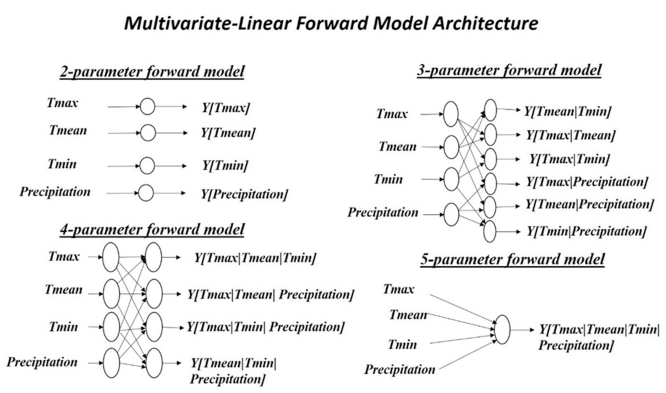
Different methodologies were used by researchers to assess the impacts of climate change on crop yields. To note, Lobell et al. (2010) proposed both statistical models and process-based crop models to predict yield responses to changes in temperature and precipitation [17]. Deryng et al. (2014) made a global gridded crop model to assess global and local climate changes [18]. Asseng et al. (2015) proposed a point-based field experiment with artificial heating and wheat yield simulation for climate change impacts [16]. Furthermore, Lobell and Field (2007) mentioned that crop yield models are scale-dependent, and global empirical/statistical models cannot reliably predict responses at sub-global scales [7]. Other possible uncertainties in a global crop yield response model are crop zone shifting in a multi-folding cropping system, decrease of crop zones due to natural and anthropogenic causes, and the variable timing (start of the season) of the growing season for different regions, etc. Therefore, in this study, we propose statistical multilinear 2-parameter, 3-parameter, 4-parameter and 5-parameter regression models to assess the climate change impacts on crop yield. These models will quantify the extent and patterns of crop yield change that could be caused by the maximum temperature (Tmax), mean temperature (Tmean), minimum temperature (Tmin) and the average precipitation change at regional scale.
In this study, we focused on one specific crop of soybean, which is mostly grown in the United States of America (USA) and has a great contribution to the US total agricultural production. We propose some significant regional soybean yield response models, which could explain the variability of crop yield due to climatic impacts. In this study, we aim to model and estimate the climate change impacts on crop yield at the regional scale by considering the irrigation status. This study will help draw the attention of the policymakers at regional and local levels for the necessary adaptations to climate change and thus enhance crop production and meet the food demand.
2. Materials and Methods
2.1. Study Area
Mississippi is one of the important agricultural states in the USA. Soybean is cultivated as a major crop in Mississippi. According to the 2020 USDA state agriculture overview of Mississippi, there is about 54 bu/acre soybean production, a total of 111,240,000 Bu, which has a value of 119,026,800 dollars ($) (https://www.nass.usda.gov/Quick_Stats/Ag_Overview/stateOverview.php?state=MISSISSIPPI) (accessed on 8 June 2021).
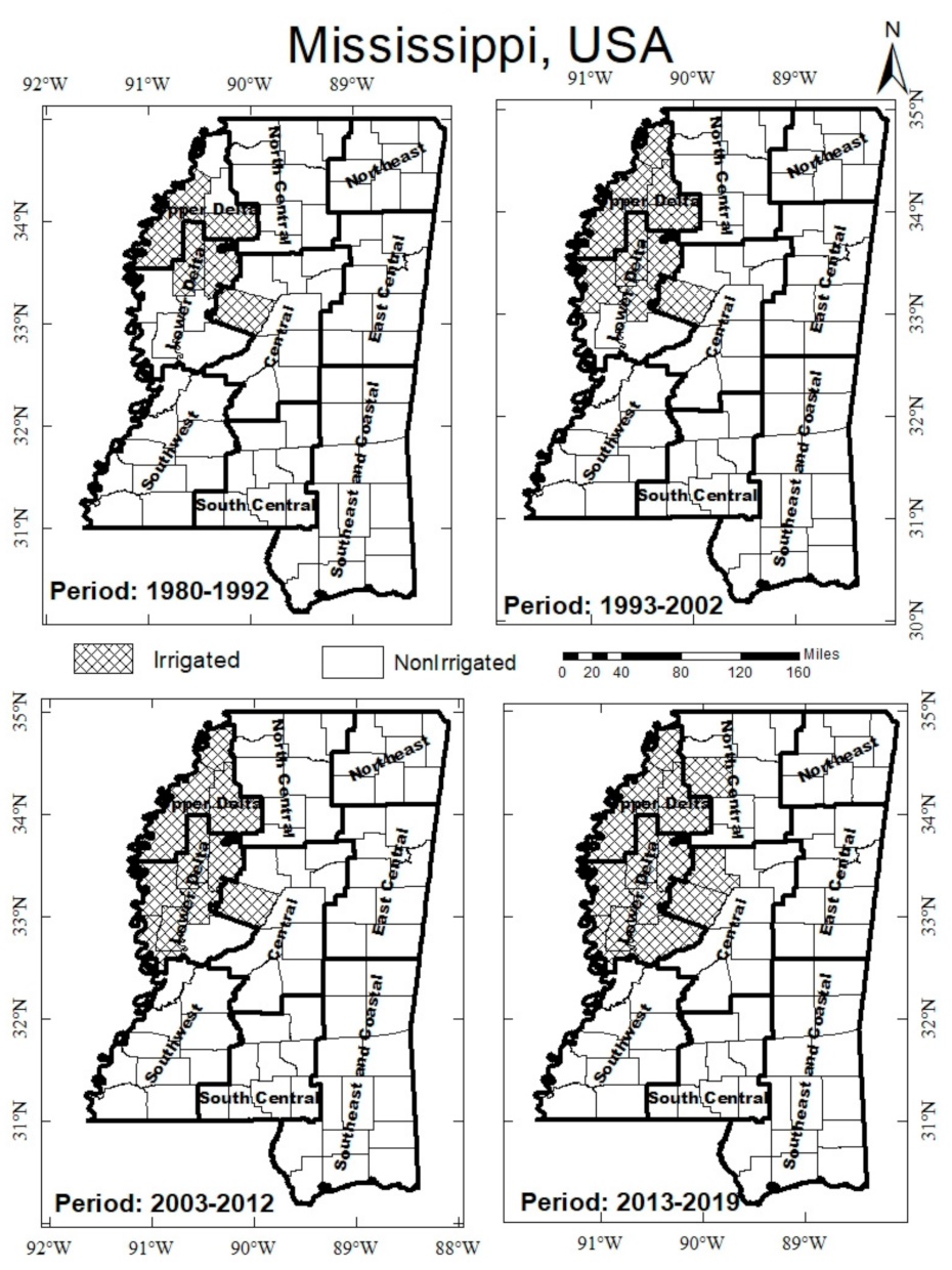
The state of Mississippi is divided into nine agricultural districts by the United States Department of Agriculture (USDA) (Figure 1). The agricultural districts are Upper Delta (district code: 10), North Central (district code: 20), Northeast (district code: 30), Lower Delta (district code: 40), Central (district code: 50), East Central (district code: 60), Southwest (district code: 70), South Central (district code: 80), and Southeast and Coastal (district code: 90). Each agricultural district consists of a number of counties. Hence, we collected the irrigation status at county level from the USDA survey report. Among the 82 counties of Mississippi, only 6 counties received irrigation facilities for soybean cultivation in 1992. Later on, 10 in 2002, 12 in 2012, and 15 in 2019, respectively, were irrigated counties (Figure 1).
2.2. Data Collection and Processing
We defined a general soybean crop season for Mississippi starting from April and ending in September based on the report of NASS (National Agricultural Statistics Service) USDA (October 2010) (https://www.nass.usda.gov/Publications/Todays_Reports/reports/fcdate10.pdf, accessed on 1 July 2020). We calculated average seasonal climate data for each year based on the crop growth period. The yearly irrigation data for the study area from 1980 to 2019 are collected from the Census of Agriculture, NASS, USDA (https://www.nass.usda.gov/Publications/AgCensus/2017/Full_Report/Volume_1,_Chapter_1_State_Level/Mississippi/, accessed on 1 July 2020). We considered a county is irrigated if it contains 40% or more irrigated croplands. In this study, we assumed this percentage is the minimum requirement to determine the county-level irrigation status for this region. Hence, the higher the percentage of the irrigation status of the crop zone for a county, the better reliability of the models for the irrigated zones.
The soybean crop yield (bushel/acre) data for the period of 1980–2019 are also collected from the USDA NASS (https://quickstats.nass.usda.gov/, accessed in 1 July 2020) and are then converted into unit kg/acre according to the USDA conversion unit (1 bushel = 27.2 Kilograms) for soybean yields. The monthly data for climatic parameters, e.g., maximum temperature (Tmax), mean temperature (Tmean), minimum temperature (Tmin), and precipitation, are collected from NOAA’s National Climatic Data Center (NCDC) (https://ncdc.noaa.gov/data-access/land-based-station-data, accessed on 1 August 2020), which gives public access to national historical weather data and metadata. More details of these data can be found at (ftp://ftp.ncdc.noaa.gov/pub/data/cirs/climdiv/, accessed on 1 August 2020).
2.3. Statistical Modeling
We applied a multilinear regression approach to model the impacts of climate change on the crop yields. We used the SAS 9.4 software for linear regression.
A general multilinear regression model (Equation (1)) is designed for different number of parameters to systematically analyze the impacts of climate change on crop yield. The modeling approach is shown in Figure 2, and the arrow direction shows the variable selection patterns for each model. The regression model is summarized using Equation (1).
where the dependent variable Yij is the crop yield at the ith location for j variables, aij is the intercept of the model, bij are the coefficient values for the ith location for j variables, and Xij is the dependent variable for the ith location for the j variables (Tmax, Tmean, Tmin, and precipitation). For two-parameter, three-parameter, four-parameter, and five-parameter models, the value of j is one, two, three, and four, respectively.
We used the adjusted R-square, AIC (Akaike’s Information Criterion), and BIC (Sawa’s Bayesian Information Criterion) to evaluate model performance and select the best regression models among the two-parameter models, three-parameter models, four-parameter models, and five-parameter models.
The adjusted R-square was used to compare models with different number of explanatory variables, as mentioned by Li and Meng [19]. This parameter could be used to identify the best model by minimizing the variability of the dependent variables with respect to the independent variables. AIC is used to find the maximum likelihood estimates of the parameters for statistical models, which is free from the ambiguities inherent in the application of the conventional hypothesis testing procedure [20]. AIC estimates a measure of the differences between a given model and a true model, and the best model is typically identified by the lowest value of AIC [19,21,22,23,24]. BIC is a criterion for the best model identification developed by Sawa [25]. It reduces the maximum likelihood selection of a model and penalizes the complexity of a model with many parameters. The algorithms used for the adjusted R-square, AIC, and BIC are Equations (2)–(4), respectively.
where y is the actual crop yield, is the predicted crop yield, is the average of the crop yield. N is the total number of observations, P is the number of parameters with intercept, SSE (sum square error) is the error variance of the fitted model, σ is a constant positive term to reduce the biasness of the model. Compared to AIC, BIC added a stronger penalty term for additional parameters in the model selection. BIC seems better than AIC as a maximum likelihood indicator for selecting nested models [26].
The best models are usually inferred based on some statistical measurements from a specific dataset [27]. Therefore, if the data are finite and noisy, we may only need to focus on a well-justified criterion to find the best model. In addition, the best model will help quantify the uncertainty, and give a framework to go beyond inferences. Hence, this study modeled the uncertainty of climate change impacts on crop yield and drew inferences about the impacts of future climate change on crop yields.
3. Results
3.1. Trend Analysis
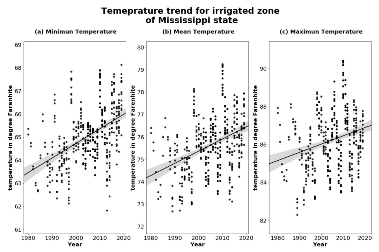
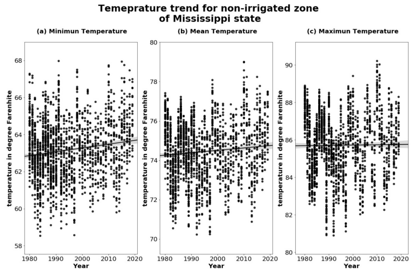
The trend of temperature for irrigated and non-irrigated zones is shown in the Figure 3 and Figure 4, respectively. In both zones, the temperature data are showing an increasing trend. The ranges of Tmin, Tmean, Tmax at the 95% confidence limits for the irrigated zone are between 63 to 66 °F, 74 to 76 °F, and 84 to 87 °F, respectively. Similarly, for the non-irrigated zones, the ranges of Tmin, Tmean, Tmax are between 62 to 64 °F, 74 to 75 °F, and 85 to 86 °F, respectively. The trends for Tmin, Tmean, and Tmax, both for irrigated and non-irrigated zones are evaluated from the Mann–Kendal test (mentioned in the Supplementary Table S1). This study found a monotonic increasing trend for Tmin, and Tmean, but no trend was observed for Tmax for the irrigated zone. In the non-irrigated zones, the Tmin showed a continuous increase, no trend for Tmean, and a decreasing trend for Tmax.
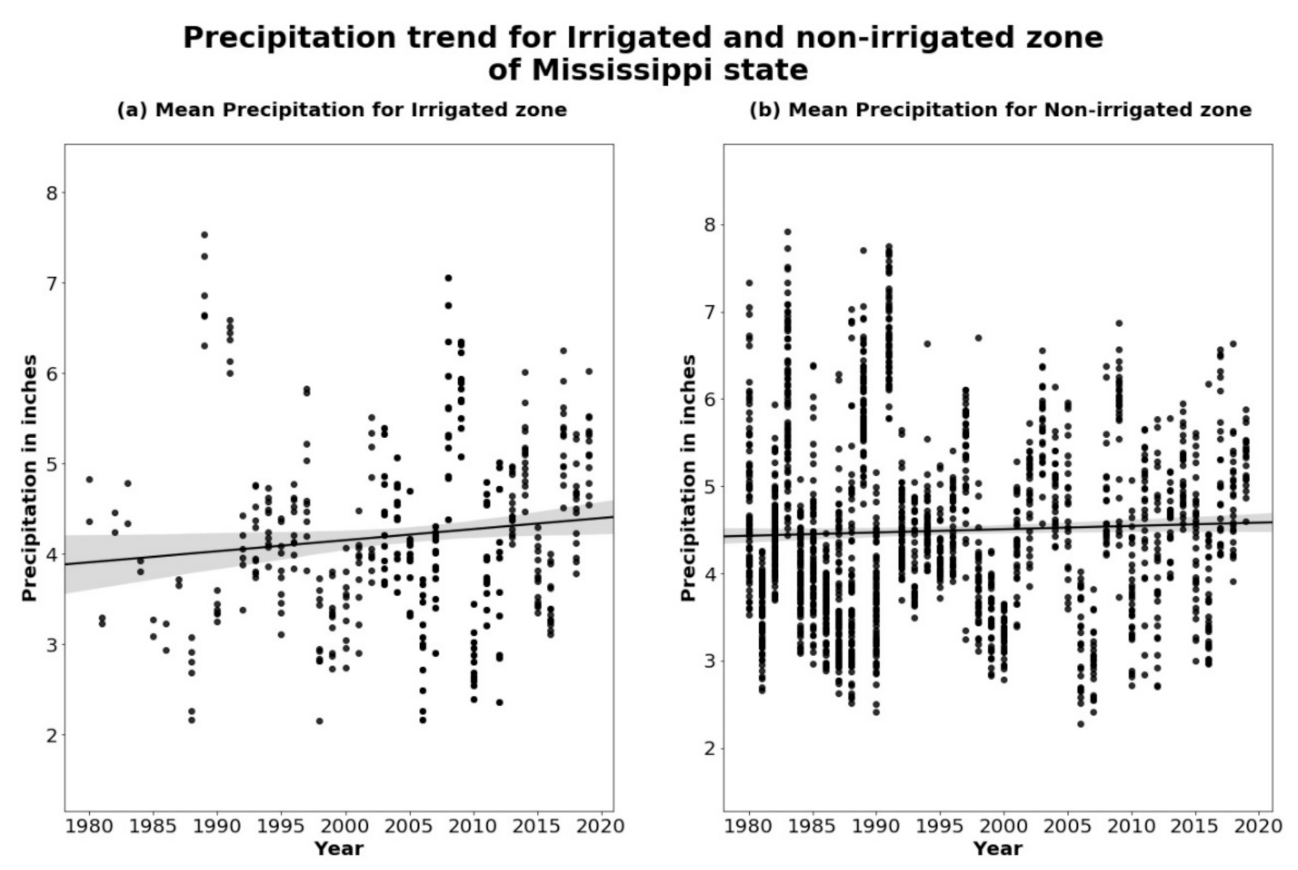
The precipitation pattern for the irrigated and non-irrigated zones is displayed in Figure 5. The range of average precipitation at the 95% confidence limit is about 3.8 to 4.5 inches for the irrigated zones, and about 4 to 4.5 inches for the non-irrigated zones. This study found both positive and negative impacts of seasonal precipitation on crop yields in different periods (e.g., −1.8 to +1.5%) and agricultural districts (e.g., −2 to +17%) for irrigated and non-irrigated zones (Table 1, Table 2, Table 3), respectively, from 1980 to 2019. Based on the Mann–Kendal test, this study found a monotonic increasing trend for precipitation in both irrigated and non-irrigated zones, which is significant at p values less than 0.00001.
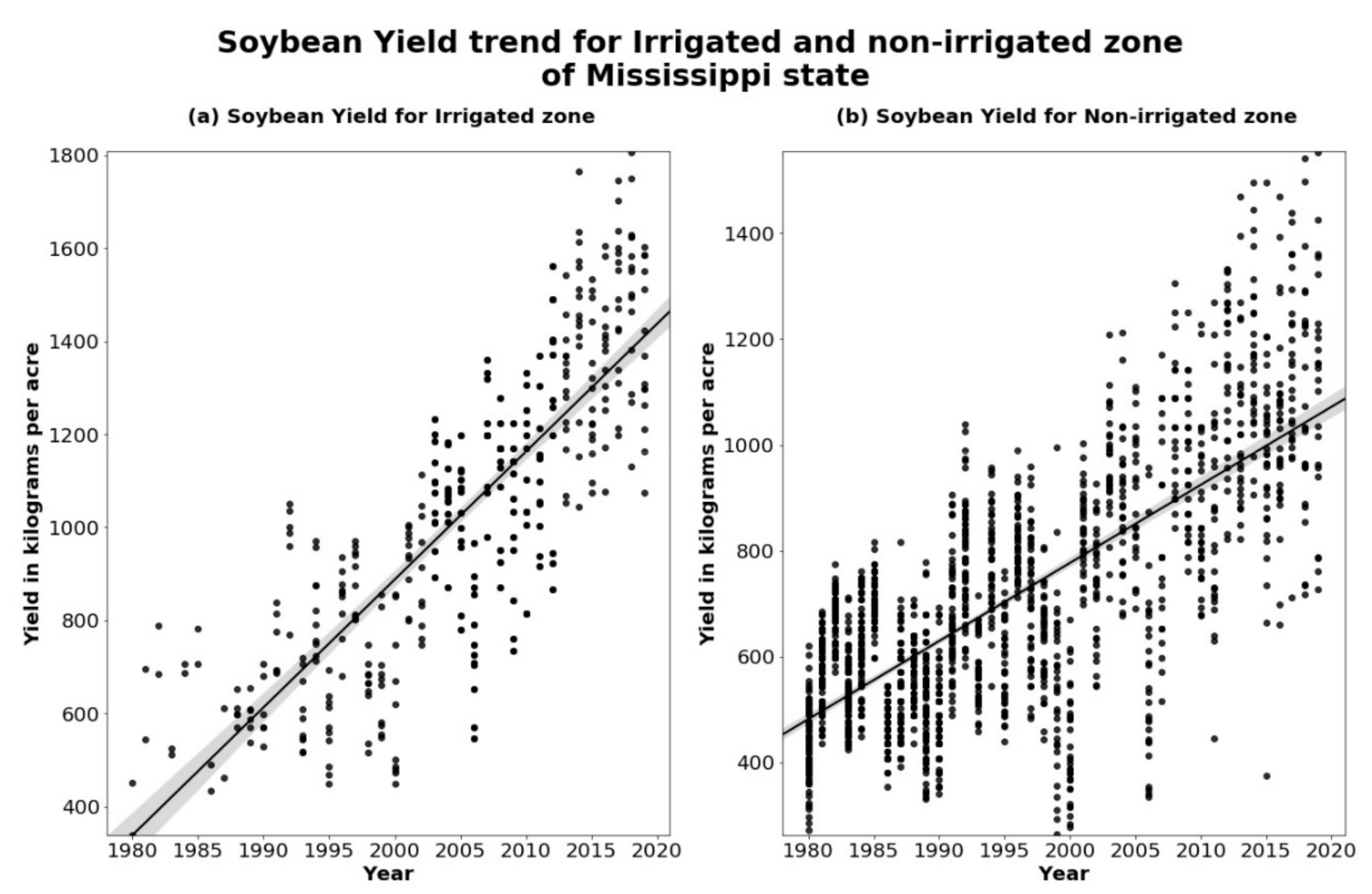
The soybean yields for both irrigated and non-irrigated regions of Mississippi indicated an increasing trend from 1980 to 2019 (Figure 6). The Mann–Kendal test also showed a significant continuous increasing trend for soybean yield in the irrigated and non-irrigated zones at the 0.00001 probability level. Due to technological improvements in the agricultural system, the soybean yield has significantly increased from 1980 to 2019. Hence, the reduction in soybean yield due to climate change is not widely observable. We may only notice the yearly crop loss that is caused by frequent climatic events, such as droughts, flooding, etc. However, the continuous climate change impacts on the crop yield become hidden.
3.2. Regional Crop Modeling for a 10-Year Period
We first used a 10-year period to model the climatic impacts on crop yields. The best models for irrigated and non-irrigated regions for each 10-year periods are reported in Table 1. The detailed results of the models are summarized in Supplementary Tables S2 and S3 for irrigated and non-irrigated zones, respectively.
For the 1980–1992 period, the model Y[Tmax,Tmin,Precipitation]92i (adjusted R-square: 65%) and Y[Tmax,Tmean,Tmin,Precipitation]92ni (adjusted R-square: 20%) are the best models to explain climate impacts in this period, for the irrigated and non-irrigated zones, respectively. Both models have the lowest BIC values compared with other models in this period. According to the model Y[Tmax,Tmin,Precipitation]92i, the covariance matrix shows that the increase of Tmax and precipitation for each crop season has a significant negative impact but a positive impact is observed for the Tmin increase on the crop yields. In contrast, for the non-irrigated zones, the model Y[Tmax,Tmean,Tmin,Precipitation]92ni also shows the same impacts on crop yield except for Tmin, which has a negative impact on crop yield for this period.
For the 1993–2002 period, the model Y[Tmax,Tmean]02i (adjusted R-square: 37%) and Y[Tmax,Tmean,Precipitation]02ni (adjusted R-square: 39%) are the best models for the irrigated and non-irrigated zones, respectively. Both models have the lowest BIC values compared with other models in this period. According to model Y[Tmax,Tmean]02i, a negative impact of Tmax and a positive impact of Tmean are reportable for irrigated zones. In contrast, the model Y[Tmax,Tmean,Precipitation]02ni shows a negative impact of Tmax but positive impacts of Tmean and precipitation, respectively, for the non-irrigated regions.
For the 2003–2012 period, the model Y[Tmax,Tmin]12i (adjusted R-square: 12%) and Y[Tmean,Tmin,Precipitation]12ni (adjusted R-square: 28%) are the best models. Both models have the lowest BIC and AIC values among the other models in this period. The covariance matrix of the model Y[Tmax,Tmin]12i shows that the increase of Tmax has a negative impact, but an increase of Tmin has a positive impact on crop yields for the irrigated zones. Otherwise, the covariance matrix of the model Y[Tmean,Tmin,Precipitation]12ni shows a negative impact of Tmean but positive impacts for Tmin and precipitation on crop yields for the non-irrigated zones.
For the 2013–2019 period, the model Y[Tmax,Tmin]19i (adjusted R-square: 29%) and Y[Tmax,Tmean,Tmin,Precipitation]19ni (adjusted R-square: 29%) are the best models for irrigated and for non-irrigated zones, respectively. Both models have the lowest BIC and AIC values compared with other models in this period. From the model Y[Tmax,Tmin]19i, a negative impact of Tmax and a positive impact of Tmin on irrigated crop yield are reported. However, from the model Y[Tmax,Tmean,Tmin,Precipitation]19ni, positive impacts for Tmean, Tmin, and precipitation but a negative impact for Tmax on non-irrigated crop yields are observed.
From each of the 10-year models, we always found the negative effect of Tmax increase and both positive and negative impacts for Tmean and Tmin, respectively. We found negative and positive impacts of precipitation on the crop yield for 1980–1992, and 1993 to 2019, respectively. This study showed the variation of climate change impacts on crop yield based on the temporal scale.
3.3. Local Crop Modeling for Agricultural Districts in Mississippi
Based on the agricultural districts, the best models for crop yield response to climatic change are summarized in Table 2, and the detailed modeling results are shown in the Supplementary Tables S4 and S5 for irrigated agricultural and non-irrigated agricultural zones, respectively. Among the nine agricultural districts of this study area, Upper Delta, Lower Delta and Central districts were irrigated zones.
In Upper Delta, Y[Tmax,Tmin]AG10i (adjusted R-square: 28%) and Y[Tmax,Tmean,Precipitation]AG10ni (adjusted R-square: 73%) are the best models to show climatic impacts on the irrigated and non-irrigated zones, respectively. Both models have the lowest AIC and BIC values compared to the other models for this Upper Delta region. Likewise, the best models for other agricultural districts were chosen.
The model Y[Tmax,Tmin]AG10i showed a negative impact of Tmax and a positive impact of Tmin in the irrigated zone of Upper Delta region. Similarly, from the best model of the Lower Delta irrigated zones, a negative impact of Tmax increase on crop yield was observed. No impacts of Tmax increase were observed for the Central irrigated zones.
On the other hand, the model Y[Tmax,Tmean,Precipitation]AG10ni indicated negative impacts of Tmax and precipitation, but a positive impact of Tmean for the non-irrigated Upper Delta regions. Similar climate change impacts were observed for the East Central, Southwest, and South Central non-irrigated crop zones.
The negative impact of Tmax increase on crop yield was noticed for other non-irrigated agricultural zones of North Central, Northeast, Lower Delta, Central, Southeast and Coastal, etc.
3.4. Regional Crop Modeling for the Whole Mississippi State
In Mississippi, the best models for crop yield response to climatic change are summarized in Table 3. The detailed model results are mentioned in the Supplementary Table S6. The model Y[Tmax,Tmean,Tmin,Precipitation]MSi (adjusted R-square: 24%) and Y[Tmax,Tmean]MSni (adjusted R-square: 14%) are explaining the best climate impacts for irrigated and for non-irrigated zones, respectively. Both models have the lowest AIC, and BIC values compared to the other models for Mississippi. According to the model Y[Tmax,Tmean,Tmin,Precipitation]MSi, a negative impact of Tmax but a positive impact of Tmean, Tmin, and precipitation were reported for the irrigated zones of Mississippi. However, the model Y[Tmax,Tmean]MSni showed a negative impact of Tmax but a positive impact of Tmean for the non-irrigated regions in Mississippi.
4. Discussion
Global warming has a significant negative impact on crop production [2,7,15]. Based on geographical locations, crops respond differently to climate changes [13]. This study monitored soybean crop and evaluated the impacts of climate change on the soybean production in Mississippi by considering irrigated and non-irrigated zones. Different temporal periods, such as six years [28], thirty years [29], and 46 years [10] have been used by researchers to identify the effects of climate on crop yield. This study used a 40-year period to monitor changes of Tmax, Tmean, Tmin, and precipitation and their impacts on soybean yields.
Temperature (e.g., Tmax, Tmean, Tmin) is a dominant factor for crop yield modeling. The increase of Tmax could cause damage to the crop yields [6,30]. A temperature increase in a crop zone directly increases the soil temperature, which may affect the plant growth indirectly. Other possible negative impacts of a temperature increase may be observable in the soil moisture content (i.e., the water holding capacity of soil), elevated carbon-dioxide (which disturbs the plant growth due to its presence in excessive amounts), multifold cropping system, and extensive agrochemicals use, etc., which also require a proper soil-water management system. This study showed that the increase of Tmax in the growth season can significantly reduce the soybean yield by 2–8% which is greater than the previous study results [7,9]. The current scenario needs attention to maintain a sustainable crop growth environment in both irrigated and non-irrigated zones. The general relationship between temperature or precipitation and crop yield was mapped (Supplementary Figures S1 and S2). Irrigated areas with lower maximum temperature typically had smaller residuals, while areas with higher maximum temperature had larger residuals; similar trends were observed in non-irrigated zones, which was not as apparent as the irrigated zones. The trends for minimum or mean temperature and precipitation were not obvious, which indicated that the modeling of climate impacts needs to be explored in alternative periods and from place to place.
Precipitation showed both significant positive and negative impacts on crop yield. This study identified the regional impacts of precipitation on crop yield. This study showed the variability about −2 to 17% of precipitation impacts on the crop yield in different agricultural districts. The crop yield reduction due to precipitation variability was also mentioned in another study [30]. Albeit, the negative impacts of temperature increase compared to precipitation is prominent in this study. However, another study showed that crops could be more sensitive to precipitation changes than temperature changes [31].
This study reported a significant increasing trend for soybean production for the state of Mississippi, which is also aligned with the local scale study of the Mississippi Delta [32]. The improvement in soybean production in this region is due to the increase in crop zone area for soybean cultivation, availability of better agrochemicals (e.g., fertilizers, pesticides, etc.), better seed quality, increase in irrigation facilities, availability of agricultural instruments to reduce manual labor, and so on. However, the decreases of crop yield due to climatic impacts were reported even with agronomic adjustments, such as addition of improved technologies and farm field management system, etc. [13]. Some factors, such as elevation, latitude and longitude, and related evapotranspiration may also influence the variability of climatic impacts on the crop yield [13]. Irrigation facilities could reduce the climate change impacts, and more crop production may result from irrigated fields compared with non-irrigated fields. Hence, more soybean production is estimated in the irrigated zones compared with the non-irrigated zones, which is similar to the results mentioned by Kukal and Imrak [33].
It is a matter of concern that future global warming will have severe impacts on crop production [34,35] and is also recognized as a threat to sustainable crop growth [13]. This study supported that the seasonal rainfall variability and seasonal temperature change have negative impacts on the crop yield [2,15,36,37,38,39]. The modeling results showed the significant negative impacts of Tmax, but positive impacts were observed for the increase of Tmean and Tmin. Hence, the increase of the daily Tmin will increase the daily Tmean and eventually could result in extreme events [40], which might negatively impact the crop yield in some situations [41]. The possible impacts of temperature change during the growing season, such as plant growth phases, pollination, maturity and harvesting, etc., ultimately could result in a reduced crop production [41].
This study gave an insight about the climate change impacts on crop yield and quantified the impacts on a regional scale. This study also showed the variability associated with the agricultural districts and state level crop yield modeling in response to climate change, which implies the necessity of future climate projection with higher spatial resolution [31]. Compared to global-scale modeling, regional and local modeling would be more reliable for crop yield responses. A local and regional model could provide high precise estimations of climate change impacts by reducing the uncertainty found in global models. The shifting of cropping areas is more identical in local modeling, which is a drawback for a global model [7]. It is also important to periodically assess the impacts of climate change on crop yields [14].
Therefore, this study could be a baseline for evaluating the impacts of climatic uncertainty on crop yield on temporal, local, and regional scales. Hence, spatial characteristics across topographically diverse regions is important to examine the climate change impacts on crop yield. [42]. The methods used in this study to assess climate change impacts on crop yield can be applicable to other regions and crops. The results of this study will provide insights for both researchers and the policymakers for climate change adaption.
5. Conclusions
This study estimated the climatic impacts on crop yield at local and regional scales with a decadal modeling approach. This study significantly complements the uncertainty and relationship between climate change and crop yield that could not be found at a global scale. The study modelled the climatic impacts on soybean yield from 1980 to 2019 by emphasizing the temperature and precipitation changes. About 2–8% reduction of soybean yield was estimated for an increase in the maximum temperature in irrigated and non-irrigated regions and within both short periods (i.e., a 10-year period) and relatively long periods (i.e., a 40-year period). The variability in precipitation showed the yield change about −2 to +17%. This study provided a baseline to show the pattern and extent of climate change and its impacts on local and regional crop yields.
Except for Tmax, precipitation and Tmean/Tmin showed diverse impacts on crop yields, spatially and temporally. In Mississippi, the impact of precipitation was not significant in 10-year modeling, but significant positive impacts were observed from the 40 years modeling for the irrigation zones; however, across different non-irrigated zones, from 1980 to 2019, precipitation showed positive effects in some non-irrigated zones but negative effects in other non-irrigated zones. Tmean and Tmin even showed more heterogeneous effects across different irrigation/non-irrigation zones and periods. Therefore, to maintain a sustainable food production, we draw the attention of researchers and policymakers to consider the climate change impacts on crop yield and make decisions across different spatial extents for both short-term and long-term goals, to adapt future climate change impacts.
Supplementary Materials
The Supplementary Materials are available online at https://0-www-mdpi-com.brum.beds.ac.uk/article/10.3390/rs13122249/s1. Figure S1. Seasonal minimum temperature (a), mean temperature (b), and maximum temperature (c), trend for Irrigated zone of Mississippi states from 1980 to 2019; Figure S2. Seasonal minimum temperature (a), mean temperature (b), and maximum temperature (c), trend for Non-irrigated zone of Mississippi states from 1980 to 2019; Figure S3. Seasonal Precipitation change for Irrigated (a) and Non-irrigated (b) zone of Mississippi states from 1980 to 2019; Figure S4. Seasonal Soybean Yield change for Irrigated (a) and Non-irrigated (b) zone of Mississippi states from 1980 to 2019; Figure S5. The grid map of Climatic variables, such as minimum temperature (a), mean temperature (b), maximum temperature (c), Precipitation (d), and residuals from best yield model for the irrigated zone of Mississippi; Figure S6. The grid map of Climatic variables, such as minimum temperature (a), mean temperature (b), maximum temperature (c), Precipitation (d), and residuals from best yield model for the non-irrigated zone of Mississippi. Table S1. The results of Mann-Kendal test for the Tmin, Tmean, Tmax, Precipitation, and Yield from time series of 1980–2019 for irrigated and non-irrigated zones of Mississippi; Table S2. The results of linear and multilinear models for each 10-year period from time series of 1980–2019 for irrigated counties in Mississippi; Table S3. The results of linear and multilinear models for each 10-year period from time series of 1980–2019 for non-irrigated county of Mississippi; Table S4. The results of linear and multilinear models for time series of 1980–2019 for irrigated agricultural districts of Mississippi; Table S5. The results of linear and multilinear models for time series of 1980–2019 for non-irrigated agricultural districts of Mississippi; Table S6. The results of linear and multilinear models for irrigated and non-irrigated zone of Mississippi of 1980–2019 period.
Author Contributions
S.A.S.: data collection and processing, GIS analysis, linear modeling, writing—original draft, reviewing and editing. Q.M.: conceptualization, methodology, data curation, investigation, supervision, writing—organization, original draft, reviewing and editing. Both authors have read and agreed to the published version of the manuscript.
Funding
This research received no external funding.
Conflicts of Interest
The authors declare no conflict of interest.
References
- Jia, G.; Shevliakova, E.; Artaxo, P.; De Noblet-Ducoudré, N.; Houghton, R.; House, J.; Kitajima, K.; Lennard, C.; Popp, A.; Sirin, A.; et al. Land-climate interactions. In Climate Change and Land: An IPCC Special Report on Climate Change, Desertification, Land Degradation, Sustainable Land Management, Food Security, and Greenhouse Gas Fluxes in Terrestrial Ecosystems; IPCC: Geneva, Switzerland, 2019; Available online: https://www.ipcc.ch/srccl/ (accessed on 12 November 2020).
- Mbow, C.; Rosenzweig, C.L.G.; Barioni, T.G.; Benton, M.; Herrero, M.; Krishnapillai, E.; Liwenga, P.; Pradhan, M.G.; Rive-ra-Ferre, T.; Sapkota, F.N.; et al. Food Security. In Climate Change and Land: An IPCC Special Report on Climate Change, Desertification, Land Degradation, Sustainable Land Management, Food Security, and Greenhouse Gas Fluxes in Terrestrial; IPCC: Geneva, Switzerland, 2019; Available online: https://www.ipcc.ch/srccl/ (accessed on 7 June 2021).
- Lobell, D.B.; Gourdji, S.M. The Influence of Climate Change on Global Crop Productivity. Plant Physiol. 2012, 160, 1686–1697. [Google Scholar] [CrossRef] [PubMed] [Green Version]
- Harrison, P.; Butterfield, R. Climate Change and Agriculture in Europe—Assessment of Impacts and Adaptation, Environmental Change Unit; Downing, T., Ed.; University of Oxford: Oxford, UK, 1995; 411p, ISBN 1-874370-09-5. [Google Scholar]
- Gadgil, S.; Rao, P.R.S.; Sridhar, S. Modeling impact of climate variability on rainfed groundnut. Curr. Sci. 1999, 76, 557–569. [Google Scholar]
- Alexandrov, V.; Hoogenboom, G. The impact of climate variability and change on crop yield in Bulgaria. Agric. For. Meteorol. 2000, 104, 315–327. [Google Scholar] [CrossRef]
- Lobell, D.B.; Field, C.B. Global scale climate–crop yield relationships and the impacts of recent warming. Environ. Res. Lett. 2007, 2. [Google Scholar] [CrossRef]
- Ray, D.K.; Gerber, J.S.; MacDonald, G.; West, P.C. Climate variation explains a third of global crop yield variability. Nat. Commun. 2015, 6, 5989. [Google Scholar] [CrossRef] [Green Version]
- Zhao, C.; Liu, B.; Piao, S.; Wang, X.; Lobell, D.B.; Huang, Y.; Huang, M.; Yao, Y.; Bassu, S.; Ciais, P.; et al. Temperature increase reduces global yields of major crops in four independent estimates. Proc. Natl. Acad. Sci. USA 2017, 114, 9326–9331. [Google Scholar] [CrossRef] [Green Version]
- Kukal, M.S.; Irmak, S. Climate-driven crop yield and yield variability and climate change impacts on the U.S. great plains agricultural production. Sci. Rep. 2018, 8, 1–18. [Google Scholar] [CrossRef] [PubMed] [Green Version]
- Kaufmann, R.K.; Snell, S.E. A Biophysical Model of Corn Yield: Integrating Climatic and Social Determinants. Am. J. Agric. Econ. 1997, 79, 178–190. [Google Scholar] [CrossRef]
- Freckleton, R.; Watkinson, A.; Webb, D.J.; Thomas, T. Yield of sugar beet in relation to weather and nutrients. Agric. For. Meteorol. 1999, 93, 39–51. [Google Scholar] [CrossRef]
- Iizumi, T.; Furuya, J.; Shen, Z.; Kim, W.; Okada, M.; Fujimori, S.; Hasegawa, T.; Nishimori, M. Responses of crop yield growth to global temperature and socioeconomic changes. Sci. Rep. 2017, 7, 1–10. [Google Scholar] [CrossRef]
- Lobell, D.B.; Schlenker, W.; Costa-Roberts, J. Climate Trends and Global Crop Production Since 1980. Science 2011, 333, 616–620. [Google Scholar] [CrossRef] [Green Version]
- Nelson, G.C.; Rosegrant, M.W.; Koo, J.; Robertson, R.; Sulser, T.; Zhu, T.; Ringler, C.; Msangi, S.; Palazzo, A.; Batka, M.M.; et al. Climate Change Impact on Agriculture and Costs of Adaptation; International Food Policy Research Institute: Washington, DC, USA, 2009; 30p, Available online: http://www.fao.org/fileadmin/user_upload/rome2007/docs/Impact_on_Agriculture_and_Costs_of_Adaptation.pdf (accessed on 8 June 2020).
- Asseng, S.; Ewert, F.; Martre, P.; Rotter, R.P.; Lobell, D.B.; Cammarano, D.; Kimball, B.A.; Ottman, M.J.; Wall, G.W.; White, J.W.; et al. Rising temperatures reduce global wheat production. Nat. Clim. Chang. 2015, 5, 143–147. [Google Scholar] [CrossRef]
- Lobell, D.B.; Burke, M.B. On the use of statistical models to predict crop yield responses to climate change. Agric. For. Meteorol. 2010, 150, 1443–1452. [Google Scholar] [CrossRef]
- Deryng, D.; Conway, D.; Ramankutty, N.; Price, J.; Warren, R. Global crop yield response to extreme heat stress under multiple climate change futures. Environ. Res. Lett. 2014, 9, 034011. [Google Scholar] [CrossRef] [Green Version]
- Li, T.; Meng, Q. Forest dynamics in relation to meteorology and soil in the Gulf Coast of Mexico. Sci. Total Environ. 2020, 702, 134913. [Google Scholar] [CrossRef]
- Akaike, H. A new look at the statistical model identification. IEEE Trans. Autom. Control 1974, 19, 716–723. [Google Scholar] [CrossRef]
- Beal, D.J. SAS Code to Select the Best Multiple Linear Regression Model for Multivariate Data Using Information Criteria. 2007. Available online: https://www.semanticscholar.org/paper/SAS-Code-to-Select-the-Best-Multiple-Linear-Model-Beal/8bdacf48dde2d77f6aa676ed79c95c6c1ad701e5 (accessed on 7 June 2021).
- Brunsdon, C.; Fotheringham, S.; Charlton, M. Geographically Weighted Regression. J. R. Stat. Soc. Ser. D Stat. 1998, 47, 431–443. [Google Scholar] [CrossRef]
- Fotheringham, A.S.; Brunsdon, C.; Charlton, M. Geographically Weighted Regression: The Analysis of Spatially Varying Relationships; John Wiley & Sons: Chichester, UK, 2002; p. 284. ISBN 978-0471496168. [Google Scholar]
- Meng, Q.; Cieszewski, C.J.; Madden, M.; Borders, B. A linear mixed-effects model of biomass and volume of trees using Landsat ETM+ images. For. Ecol. Manag. 2007, 244, 93–101. [Google Scholar] [CrossRef]
- Sawa, T. Information Criteria for Discriminating among Alternative Regression Models. Econometrica 1978, 46, 1273–1291. [Google Scholar] [CrossRef] [Green Version]
- Wang, Y.; Liu, Q. Comparison of Akaike information criterion (AIC) and Bayesian information criterion (BIC) in selection of stock–recruitment relationships. Fish. Res. 2006, 77, 220–225. [Google Scholar] [CrossRef]
- Burnham, K.P.; Anderson, D.R. Multimodel Inference: Understanding AIC and BIC in Model Selection. Sociol. Methods Res. 2004, 33, 261–304. [Google Scholar] [CrossRef]
- Lobell, D.B.; Asner, G.P. Climate and management contributions to recent trends in US agricultural yields. Science 2003, 299, 1032. [Google Scholar] [CrossRef]
- Leng, G.; Zhang, X.; Huang, M.; Asrar, G.R.; Leung, L.R. The Role of Climate Covariability on Crop Yields in the Conterminous United States. Sci. Rep. 2016, 6, 33160. [Google Scholar] [CrossRef]
- Cai, X.; Wang, D.; Laurent, R. Impact of Climate Change on Crop Yield: A Case Study of Rainfed Corn in Central Illinois. J. Appl. Meteorol. Clim. 2009, 48, 1868–1881. [Google Scholar] [CrossRef]
- Kang, Y.; Khan, S.; Ma, X. Climate change impacts on crop yield, crop water productivity and food security—A review. Prog. Nat. Sci. 2009, 19, 1665–1674. [Google Scholar] [CrossRef]
- Shammi, S.A.; Meng, Q. Use time series NDVI and EVI to develop dynamic crop growth metrics for yield modeling. Ecol. Indic. 2021, 121, 107124. [Google Scholar] [CrossRef]
- Kukal, M.S.; Irmak, S. Irrigation-limited yield gaps: Trends and variability in the United States post-1950. Environ. Res. Commun. 2019, 1, 061005. [Google Scholar] [CrossRef]
- Mavromatis, T. Crop–climate relationships of cereals in Greece and the impacts of recent climate trends. Theor. Appl. Clim. 2015, 120, 417–432. [Google Scholar] [CrossRef]
- Innes, P.; Tan, D.; Van Ogtrop, F.; Amthor, J. Effects of high-temperature episodes on wheat yields in New South Wales, Australia. Agric. For. Meteorol. 2015, 208, 95–107. [Google Scholar] [CrossRef]
- Challinor, A.J.; Watson, J.; Lobell, D.B.; Howden, S.M.; Smith, D.R.; Chhetri, N. A meta-analysis of crop yield under climate change and adaptation. Nat. Clim. Chang. 2014, 4, 287–291. [Google Scholar] [CrossRef]
- Ruane, A.C.; Rosenzweig, C.; Asseng, S.; Boote, K.J.; Elliott, J.; Ewert, F.; Jones, J.W.; Martre, P.; McDermid, S.P.; Müller, C.; et al. An AgMIP framework for improved agricultural representation in integrated assessment models. Environ. Res. Lett. 2017, 12, 125003. [Google Scholar] [CrossRef] [PubMed]
- Parry, M.L.; Rosenzweig, C.; Iglesias, A.; Livermore, M.; Fischer, G. Effects of climate change on global food production under SRES emissions and socio-economic scenarios. Glob. Environ. Chang. 2004, 14, 53–67. [Google Scholar] [CrossRef]
- Wheeler, T.; Von Braun, J. Climate Change Impacts on Global Food Security. Science 2013, 341, 479–485. [Google Scholar] [CrossRef] [PubMed]
- Global Climate Projections; Cambridge University Press: Cambridge, UK; New York, NY, USA, 2007; Available online: https://www.fws.gov/southwest/es/documents/R2ES/LitCited/LPC_2012/Meehl_et_al_2007.pdf (accessed on 8 June 2020).
- Hatfield, J.L.; Prueger, J.H. Temperature extremes: Effect on plant growth and development. Weather. Clim. Extrem. 2015, 10, 4–10. [Google Scholar] [CrossRef] [Green Version]
- Jones, P.G.; Thornton, P.K. The potential impacts of climate change on maize production in Africa and Latin America in 2055. Glob. Environ. Chang. 2003, 13, 51–59. [Google Scholar] [CrossRef]
Figure 1.
The irrigated and non–irrigated zones in Mississippi, USA from 1980 to 2019. Nine agricultural districts categorized by USDA.
Figure 1.
The irrigated and non–irrigated zones in Mississippi, USA from 1980 to 2019. Nine agricultural districts categorized by USDA.

Figure 2.
The model architecture of multivariate linear regression. The two–parameter, three–parameter, four–parameter, and five–parameter models are considered.
Figure 2.
The model architecture of multivariate linear regression. The two–parameter, three–parameter, four–parameter, and five–parameter models are considered.

Figure 3.
Trends for (a) seasonal minimum temperature, (b) mean temperature, and (c) maximum temperature, for the irrigated zones of the Mississippi State from 1980 to 2019.
Figure 3.
Trends for (a) seasonal minimum temperature, (b) mean temperature, and (c) maximum temperature, for the irrigated zones of the Mississippi State from 1980 to 2019.

Figure 4.
Trends for (a) seasonal minimum temperature, (b) mean temperature, and (c) maximum temperature, trend for non–irrigated zones of the Mississippi State from 1980 to 2019.
Figure 4.
Trends for (a) seasonal minimum temperature, (b) mean temperature, and (c) maximum temperature, trend for non–irrigated zones of the Mississippi State from 1980 to 2019.

Figure 5.
Trends for seasonal precipitation change for (a) irrigated zones and (b) non–irrigated zones of the Mississippi State from 1980 to 2019.
Figure 5.
Trends for seasonal precipitation change for (a) irrigated zones and (b) non–irrigated zones of the Mississippi State from 1980 to 2019.

Figure 6.
Trends for seasonal soybean yield change for (a) irrigated zones and (b) non–irrigated zones of the Mississippi State from 1980 to 2019.
Figure 6.
Trends for seasonal soybean yield change for (a) irrigated zones and (b) non–irrigated zones of the Mississippi State from 1980 to 2019.


Table 1.
The results of the best temporal linear and multilinear models for each 10-year period from time series of 1980–2019 for the irrigated and non-irrigated counties of Mississippi.
Table 1.
The results of the best temporal linear and multilinear models for each 10-year period from time series of 1980–2019 for the irrigated and non-irrigated counties of Mississippi.
| Model Name | Intercept | Model Slope for Different Parameters | Adjusted R-Square | BIC | AIC | |||
|---|---|---|---|---|---|---|---|---|
| Tmax | Tmean | Tmin | Precipitation | |||||
| Y[Tmax,Tmin,Precipitation]92i | 264.87 | −6.36 | 5.04 | −4.80 | 0.65 | 120.2 | 117.7 | |
| Y[Tmax,Tmean]02i | 114.50 | −8.40 | 8.43 | . | . | 0.37 | 318.2 | 316.1 |
| Y[Tmax,Tmin]12i | −82.04 | −2.04 | . | 4.57 | . | 0.12 | 456.1 | 453.9 |
| Y[Tmax,Tmin]19i | 143.52 | −4.80 | . | 4.89 | . | 0.29 | 357.5 | 355.3 |
| Y[Tmax,Tmean,Tmin,Precipitation]92ni | 68.50 | −4.54 | 6.51 | −2.23 | -0.42 | 0.20 | 2737.0 | 2734.9 |
| Y[Tmax,Tmean,Precipitation]02ni | 119.74 | −6.20 | 5.82 | . | 0.63 | 0.39 | 1128.9 | 1126.8 |
| Y[Tmean,Tmin,Precipitation]12ni | −5.69 | . | −4.34 | 5.67 | 0.95 | 0.28 | 1004.3 | 1002.1 |
| Y[Tmax,Tmean,Tmin,Precipitation]19ni | 75.79 | −4.34 | 2.97 | 1.70 | 1.20 | 0.17 | 728.8 | 726.5 |
In the model names, the notation 92 is for the time 1980 to 1992; 02 is for 1993–2002; 12 is for 2003 to 2012; and 19 is for 2013 to 2019 and “i” is for irrigated zone and “ni” is for non-irrigated zone.
Table 2.
The results of the best linear and multilinear models from the time series of 1980–2019 for irrigated and non-irrigated agricultural districts in Mississippi.
Table 2.
The results of the best linear and multilinear models from the time series of 1980–2019 for irrigated and non-irrigated agricultural districts in Mississippi.
| Model Name | Intercept | Model Slope for Different Parameters | Adjusted R-Square | BIC | AIC | ||||
|---|---|---|---|---|---|---|---|---|---|
| Tmax | Tmean | Tmin | Precipitation | ||||||
| Y[Tmax,Tmin]AG10i | 20.51 | −4.64 | . | 6.38 | . | 0.28 | 886.9 | 884.8 | |
| Y[Tmax,Tmean,Tmin]AG40i | −175.04 | −4.88 | 3.55 | 5.63 | . | 0.26 | 1053.4 | 1051.2 | |
| Y[Tmin,Precipitation]AG50i | −210.18 | . | . | 3.61 | 3.43 | 0.13 | 225.8 | 223.3 | |
| Y[Tmax,Tmean,Precipitation]AG10ni | 116.91 | −7.17 | 7.10 | . | −2.72 | 0.73 | 89.1 | 86.1 | |
| Y[Tmax,Tmean,Precipitation]AG20ni | 8.49 | −4.61 | 5.46 | . | 1.49 | 0.20 | 1310.0 | 1307.9 | |
| Y[Tmax,Tmean]AG30ni | 40.42 | −4.17 | 4.63 | . | . | 0.15 | 1218.0 | 1216.0 | |
| Y[Tmax,Tmean,Tmin]AG40ni | 72.87 | −4.72 | 7.42 | −3.10 | . | 0.09 | 432.7 | 430.4 | |
| Y[Tmax,Tmean,Precipitation]AG50ni | −130.17 | −3.26 | 5.72 | . | 2.41 | 0.22 | 1114.0 | 1111.8 | |
| Y[Tmax,Tmean,Precipitation]AG60ni | 16.36 | −10.11 | 11.89 | . | −1.71 | 0.30 | 964.3 | 962.1 | |
| Y[Tmax,Tmean,Precipitation]AG70ni | −35.22 | −9.86 | 12.25 | . | −1.82 | 0.36 | 799.6 | 797.4 | |
| Y[Tmax,Tmin,Precipitation]AG80ni | 16.53 | −3.88 | . | 5.57 | −2.26 | 0.29 | 580.7 | 578.4 | |
| Y[Tmax,Tmean]AG90ni | 124.33 | −1.48 | 0.35 | . | . | 0.08 | 650.2 | 648.1 | |
In the model names, the notations AG10, AG20, AG30, AG40, AG50, AG60, AG70, AG80, and AG90 are for the agricultural district codes 10, 20, 30, 40, 50, 60, 70, 80, and 90, respectively; the notation “i” is for irrigated zone and “ni” is for non-irrigated zone in an agricultural district.
Table 3.
The results of the best multilinear models from the time series of 1980–2019 for the irrigated and non-irrigated zones in Mississippi.
Table 3.
The results of the best multilinear models from the time series of 1980–2019 for the irrigated and non-irrigated zones in Mississippi.
| Model Name | Intercept | Model Slope for Different Parameters | Adjusted R-Square | BIC | AIC | |||
|---|---|---|---|---|---|---|---|---|
| Tmax | Tmean | Tmin | Precipitation | |||||
| Y[Tmax,Tmean,Tmin,Precipitation]MSi | −144.86 | −3.93 | 2.96 | 4.48 | 1.48 | 0.24 | 2218.3 | 2216.2 |
| Y[Tmax,Tmean]MSni | 53.55 | −4.47 | 4.77 | . | . | 0.14 | 7486.6 | 7484.6 |
In the model names, the notation MS is for Mississippi State; the notation “i” is for irrigated zones and “ni” for non-irrigated zones in the Mississippi State.
Publisher’s Note: MDPI stays neutral with regard to jurisdictional claims in published maps and institutional affiliations. |
© 2021 by the authors. Licensee MDPI, Basel, Switzerland. This article is an open access article distributed under the terms and conditions of the Creative Commons Attribution (CC BY) license (https://creativecommons.org/licenses/by/4.0/).
Share and Cite
MDPI and ACS Style
Shammi, S.A.; Meng, Q. Modeling the Impact of Climate Changes on Crop Yield: Irrigated vs. Non-Irrigated Zones in Mississippi. Remote Sens. 2021, 13, 2249. https://0-doi-org.brum.beds.ac.uk/10.3390/rs13122249
AMA Style
Shammi SA, Meng Q. Modeling the Impact of Climate Changes on Crop Yield: Irrigated vs. Non-Irrigated Zones in Mississippi. Remote Sensing. 2021; 13(12):2249. https://0-doi-org.brum.beds.ac.uk/10.3390/rs13122249
Chicago/Turabian StyleShammi, Sadia Alam, and Qingmin Meng. 2021. "Modeling the Impact of Climate Changes on Crop Yield: Irrigated vs. Non-Irrigated Zones in Mississippi" Remote Sensing 13, no. 12: 2249. https://0-doi-org.brum.beds.ac.uk/10.3390/rs13122249
Note that from the first issue of 2016, this journal uses article numbers instead of page numbers. See further details here.