Article

Multiscale Semantic Feature Optimization and Fusion Network for Building Extraction Using High-Resolution Aerial Images and LiDAR Data

by
Qinglie Yuan
1,2,*,
Helmi Zulhaidi Mohd Shafri
1,
Aidi Hizami Alias
1 and
Shaiful Jahari bin Hashim
1
1
Department of Civil Engineering and Geospatial Information Science Research Centre (GISRC), Faculty of Engineering, Universiti Putra Malaysia (UPM), Serdang 43400, Selangor, Malaysia
2
Department of Geographic Information and Remote Sensing Research Centre, School of Civil and Architecture Engineering, Panzhihua University, Panzhihua 617000, China
*
Author to whom correspondence should be addressed.
Remote Sens. 2021, 13(13), 2473; https://0-doi-org.brum.beds.ac.uk/10.3390/rs13132473
Submission received: 15 May 2021 / Revised: 15 June 2021 / Accepted: 21 June 2021 / Published: 24 June 2021
(This article belongs to the Special Issue Big Remotely Sensed Data)

Abstract

:
Automatic building extraction has been applied in many domains. It is also a challenging problem because of the complex scenes and multiscale. Deep learning algorithms, especially fully convolutional neural networks (FCNs), have shown robust feature extraction ability than traditional remote sensing data processing methods. However, hierarchical features from encoders with a fixed receptive field perform weak ability to obtain global semantic information. Local features in multiscale subregions cannot construct contextual interdependence and correlation, especially for large-scale building areas, which probably causes fragmentary extraction results due to intra-class feature variability. In addition, low-level features have accurate and fine-grained spatial information for tiny building structures but lack refinement and selection, and the semantic gap of across-level features is not conducive to feature fusion. To address the above problems, this paper proposes an FCN framework based on the residual network and provides the training pattern for multi-modal data combining the advantage of high-resolution aerial images and LiDAR data for building extraction. Two novel modules have been proposed for the optimization and integration of multiscale and across-level features. In particular, a multiscale context optimization module is designed to adaptively generate the feature representations for different subregions and effectively aggregate global context. A semantic guided spatial attention mechanism is introduced to refine shallow features and alleviate the semantic gap. Finally, hierarchical features are fused via the feature pyramid network. Compared with other state-of-the-art methods, experimental results demonstrate superior performance with 93.19 IoU, 97.56 OA on WHU datasets and 94.72 IoU, 97.84 OA on the Boston dataset, which shows that the proposed network can improve accuracy and achieve better performance for building extraction.

Graphical Abstract

1. Introduction

Building extraction is important for updating geographic information and urban construction using remote sensing technology. Building information has been used in a wide range of domains such as urban management and expansion, intelligent city construction, 3D semantic modeling, autonomous driving, and traffic navigation [1,2,3,4,5,6]. Accurate building spatial information can provide vital decisions and analyses for urbanization, especially land use and cover. In the maintenance of urban geographic information systems, there is often a massive workload involved in updates and modifications due to frequent urban reconstruction. It is obvious to develop automatic building extraction methods from remote sensing data instead of manual annotation to avoid waste of time and cost. However, buildings have multi-scale and complex background in remote sensing data. Automatic and precise extraction of buildings is still challenging in the research frontier of remote sensing.
Many approaches have been applied in building extraction by constructing discriminative features from 2D and 3D data, such as satellite or aerial images [7,8,9] and LiDAR point clouds [10,11,12] or data fusion [13,14,15]. Nonetheless, these methods are mainly based on the low- or middle-level feature depending on the specific design of prior knowledge and are sensitive to parameters, while the types of buildings exhibit diversity and distribute irregularly, which hardly separate from the complex scenes with specified threshold setting [11,12,13,14]. Due to environmental factors, the building areas are prone to present shadow, occlusion and solar radiation, and noise, causing confusion with other ground objects. Therefore, the completion of robust and precise extraction is limited to using shallow features. The methods mentioned above can effectively extract specific building regions using hand-crafted features.
In recent years, deep learning technology has achieved revolutionary development in computer vision research such as semantic segmentation, object detection, and data fusion. In addition, the deep learning algorithm is also applied in engineering, such as in the three-dimensional (3D) reconstruction of large-scale, concrete-filled steel tubes [15]. In particular, deep neural networks can compensate for the drawbacks of hand-crafted features-based methods, which fail to extract high-level features and rich semantic information. In the deep learning frameworks, fully convolutional neural networks (FCNs) can automatically learn features of different levels through training datasets [16,17]. Subsequently, the improved FCN algorithms have obtained state-of-the-art results for building segmentation using remote sensing data [18,19,20]. However, these strategies do not consider feature selection when reusing earlier information, which could hamper the performance of the CNNs. Therefore, the attention mechanism was introduced into the FCN model using high-resolution aerial imagery to select spatial and channel information adaptively [19,20,21]. To construct multi-scale context information, some pyramid pooling models and encoder-decoder structures are used to optimize the network architecture. Furthermore, some network models synthesized the advantages of multi-modal data, including multispectral images and LiDAR data, to improve the accuracy of building extraction [22,23,24].
Although the above-proposed methods can effectively improve the performance of FCNs and achieved the results of pixel-wise building extraction, there are still challenges to be addressed. First, many deep learning models are trained based on natural scene images, but the data obtained from long-distance remote sensing platforms with complex backgrounds and long distances are not suitable for remote sensing ground object interpretation [25]. Although the combination of multi-source data (such as images and lidar data) can improve the accuracy of building extraction, multi-modal data have different advantages and characteristics, and thus an effective means of fusion must be explored. Many methods do not effectively integrate these features to enhance the network generalization ability. Buildings exhibit scale variability in remote sensing images because of diverse image resolution and arbitrary size. Convolutional operation with the fixed filter receptive fields could not generate discriminative representations due to the scale variability of different buildings in remote sensing images. Some modules aim to establish multiscale semantic features adopting pyramid pooling structures or encoder-decoder architecture [26,27,28,29,30,31]. The local and global semantic information provides competitive descriptors for scale variability. However, these contextual descriptors focus on local feature dependence but ignore the global correlation existing in multiscale regions and across levels, causing semantic inconsistency for feature construction and interpretation mistakes due to high intra-class and low inter-class variabilities. Hence, the multiscale contextual information needs to adaptively enhance the consistency of semantic features for intra-class regions and suppress background information. Second, buildings possess rich geometric details, such as sharp corners, edges, and some tiny structures. Pyramid pooling models working on high-level feature maps with coarse resolution struggle to capture small objects because pooling operation dramatically reduces image resolution. Low-level features contain irrelevantly redundant information without semantic guidance in encoder-decoder architecture, which probably hinders accurate boundary segmentation [22]. Semantic difference from across-level features brings segmentation ambiguity and reduces feature fusion efficiency.
To solve the above issues, we proposed an end-to-end FCN model architecture based on a residual network structure using high-resolution aerial images and LiDAR data. The residual network can extract high-level features and effectively alleviate the problem of accuracy degradation as the depth of the network increases. Two novel modules are applied to the model to obtain multi-scale global context information and refine features.
The main contributions of this paper are summarized as follows:
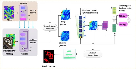
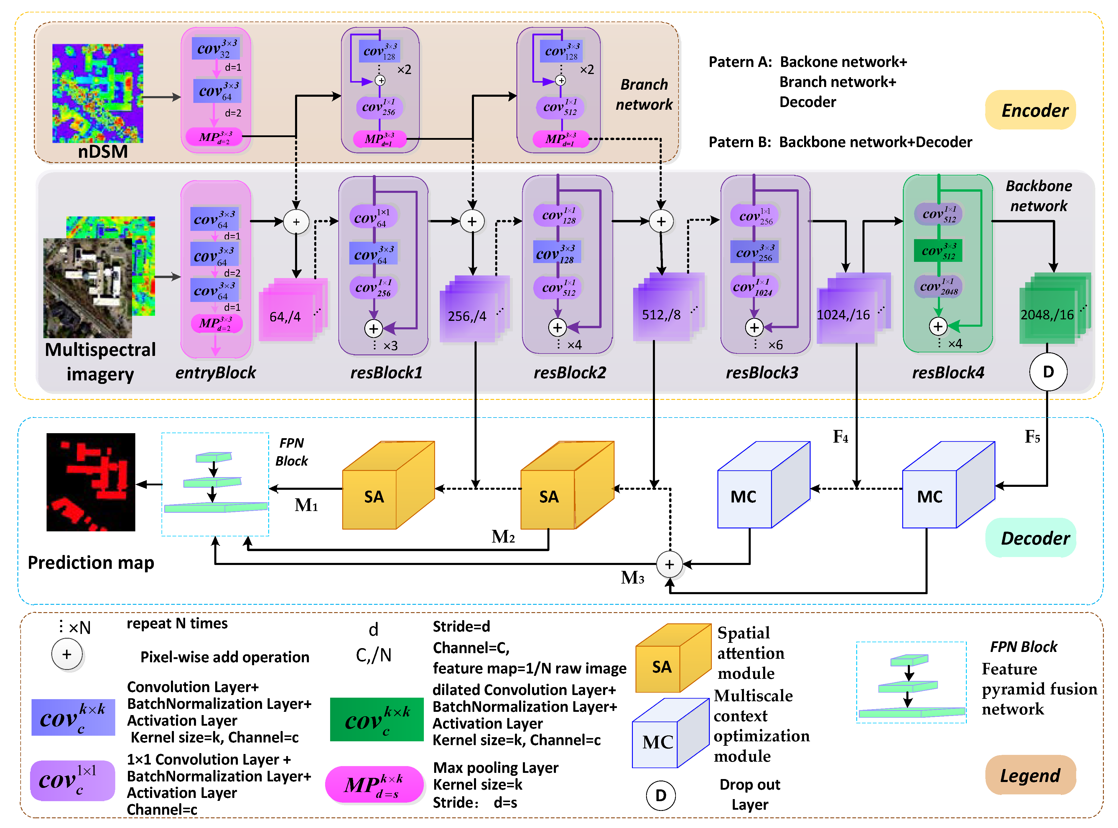
  • We redesigned the FCN architecture using modified residual networks (ResNet50) as the backbone encoder network to extract features and obtain a large receptive field. The residual branch network assists the backbone network to convert features and enhance multi-modal data fusion. Feature pyramid structures with the proposed decoder modules effectively optimize and fuse across-level multiscale features.
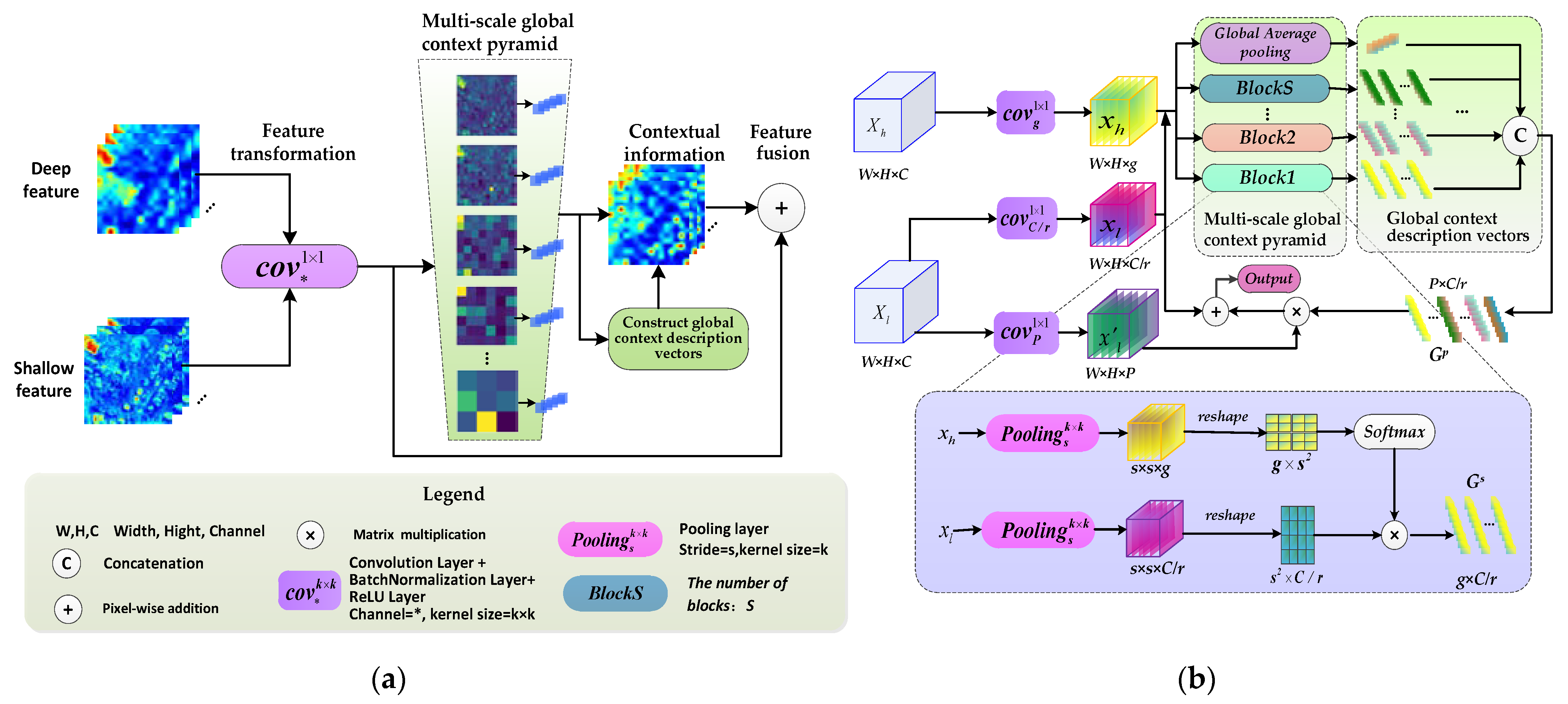
  • The proposed multiscale context optimization module (MCOM) can obtain multiscale global semantic features and generate the contextual representations of different local regions to adaptively enhance the semantic consistency of intra-class and the discrepancy of inter-class for multiscale building regions.
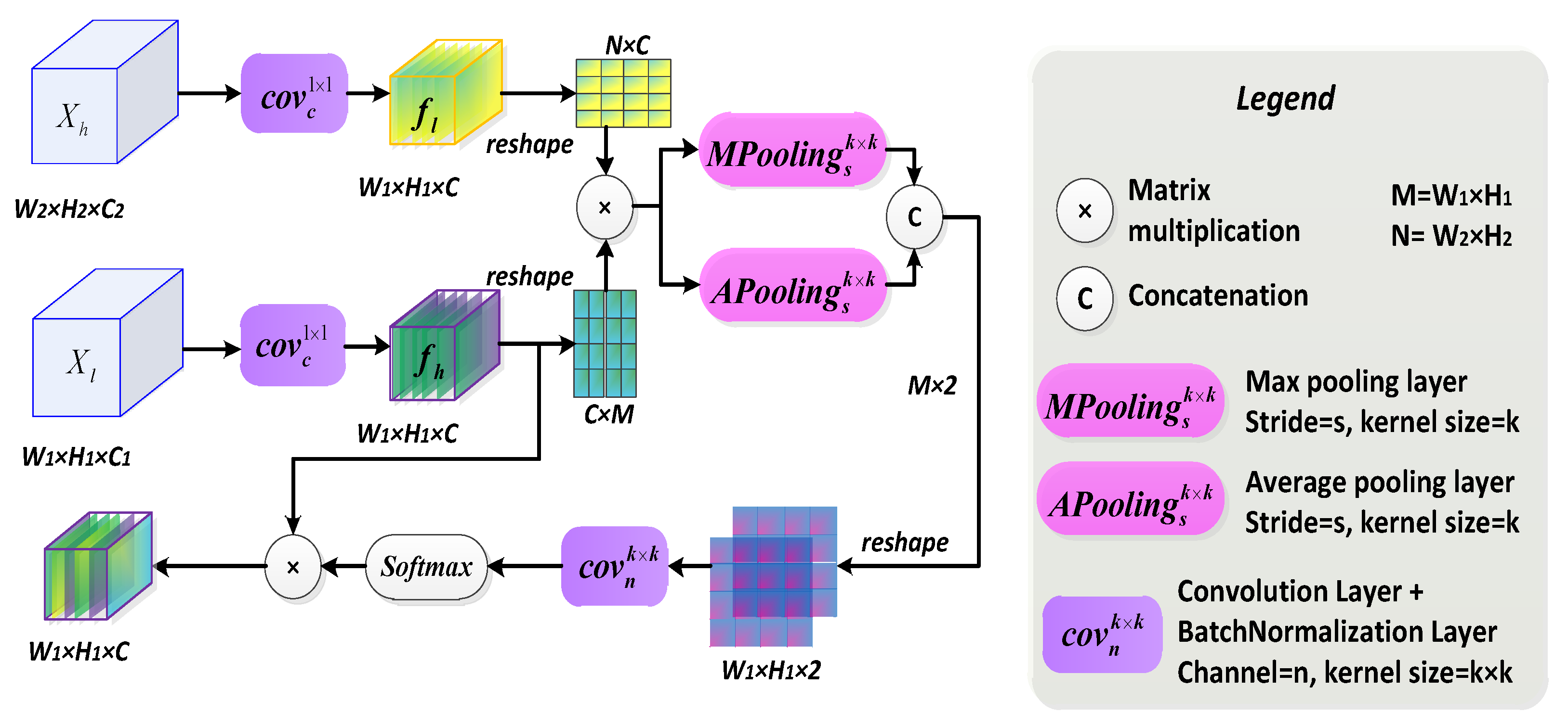
  • A semantic guided spatial attention module (SAM) is developed that leverages features from shallow and deep layers. This module can generate an attention map using across-level features to acquire long-distance correlation for pixel-wise spatial position and refine low-level features by filtering redundant information.

2. Related Work

2.1. Contextual Feature Aggregation

Building extraction in remote sensing images can be regarded as a binary classification processing by using FCNs. In the complex background, rich context information provides crucial clues for feature selection. ParseNet [32] adopts a simple solution to obtain global features through GAP (global average pooling). The pyramid pooling model has a pyramid structure to generate multiscale context vectors. For example, PSPNet employs the spatial pyramid pooling model to aggregate the feature vectors of different regions, but after multiple parallel pooling layers, the resolution and detail features of objects are reduced. Inspired by the spatial pyramid pooling model (SPP), ASPP uses convolution of various dilated rates to capture context and keep the resolution, while the effective wights of convolution kernel decrease with large dilated rates [31], which is harmful for large building segmentation. Moreover, these modules all ignore the correlations of different regions and semantic levels for object segmentation.
Previous works combine encoder-decoder architecture to recover detail features and capture multiscale context simultaneously by employing skip-connections and the pyramid pooling model module [27]. However, low-level features in the decoder lack semantic information, while high-level context features have limited spatial information, which cannot effectively fuse multiple features and leverage benefits between different hierarchical features by merely simple channel concatenation or pixel-summation. In this work, we design decoder modules to optimize the features from encoders at different stages of the network. Deep and middle features are reused to generate multiscale semantic descriptions and obtain rich global context. Shallow features are recalibrated by the spatial attention mechanism to keep semantic consistent with deep features.

2.2. Attention Mechanism

The attention mechanism aims to select the information that is more critical to the current tasks. Many attention mechanism models have been applied to deep convolution neural networks to optimize the process of feature extraction. For instance, the Squeeze-and-Excitation Networks (SENet) [33] uses GAP operation to obtain global representation along the channel axis and automatically learn the weight parameters to remark each feature. The convolutional block attention module (CBAM) [34] combines the attention mechanism in channel and space. Similarly, the Dual Attention Network (DANet) [35] proposes position attention and channel attention mechanism from enhancing the global feature fusion and the correlation between semantic features. To capture long-range dependencies, Non-local Neural Networks (NLnet) [36] transform the features to linear embeddings via conv1×1 and then calculate the global attention value for each pixel. However, the high cost of computing and GPU memory occupation limit its application.
Many methods have improved the previous work to reduce the computational cost of similarity matrix in non-local attention modules, such as APNB and Ccnet [37,38]. However, this operation ignores the semantic gap between different level feature maps by concatenation or sum directly. Due to the lack of semantic information of low-level features, the fused feature map easily generates redundant information and noise. In this work, inspired by CBAM [34] and NLnet [36], we design a spatial attention decoder to refine shallow features and filter redundant information. To alleviate the semantic feature gap, deep features and shallow features are cascaded to construct the similarity map recalibrating the shallow features.

2.3. Multiscale Feature Fusion

In FCNs, the reconstruction of a high-resolution feature map is crucial for accurate pixel-level extraction, which requires both enhanced semantic information and fine-grained spatial information to achieve classification and divide the precise boundaries in the foreground. Some methods employ the encoder-decoder method, such as U-Net structure [29], to fuse the multi-level feature maps from the backbone network by skip-connection. The decoder requires up-sampling, such as deconvolution and bilinear interpolation [28], to gradually fuse and recover resolution from high-level to low-level feature maps.
Similarly, some methods construct the feature pyramid to merge corresponding features from multiple resolutions, reducing the computational cost by adding the feature maps of different levels after up-sampling. In this network, the feature pyramid model is applied to fuse hierarchical features after the decoder and generate a prediction map with rich semantic and spatial information.

3. Proposed Method

The developed network based on residual FCNs aims to build the encoder-decoder architecture using multi-modal high-spatial resolution remote sensing data for building extraction. A modified residual model as a baseline with an auxiliary network branch encodes hierarchical features. Two novel modules as decoders are proposed and effectively integrate the deep and shallow features in different stages. Finally, a binary classification map can be generated for the prediction of buildings. We first described the overall network framework, and then the proposed decoder architecture was introduced in subsequent sections.

3.1. Network Framework

The proposed model architecture consists of the backbone network, branch networks, building encoder, and decoder architecture, as shown in Figure 1. For the encoder, the modified ResNet50 [39] as the backbone network is used to generate the multi-level features, while the branch network is composed of stacked residual convolution blocks to obtain auxiliary information and enhance feature fusion. Multispectral images were fed into the backbone network. Meanwhile, the feature of LiDAR-generated nDSM extracted from the branch network is transmitted into the backbone in different stages.
Concretely, the backbone network contains an entry block and four residual convolution blocks (resBlock1~resBlock4), as illustrated in Figure 1. At the beginning of the backbone network, ResNet50 was modified in the entry block by stacking three 3 × 3 convolutions following 3 × 3 max pooling instead of 7 × 7 convolution, where 64 feature maps can be obtained through the first layer convolution, and the spatial resolution of the last layer is one-fourth of its input resolution. This modification allows the model to support multiple channel inputs and reduce parameters using small convolutional kernels. A drop-out layer replaces the fully connected layers to prevent overfitting. Each residual block applies shortcut and bottleneck structures to avoid degradation of training accuracy. Rectified linear unit (ReLU) as an activation layer is used in the model. Downsampling followed the first convolutional layer in the residual block2 with a stride of two but is removed in residual block4. Instead, the last residual block using atrous convolutions (3 × 3 kernels, 2 dilated rate) simultaneously ensures a large receptive field and constant spatial resolution for deep level feature maps to reduce loss of spatial information. Therefore, the spatial resolution of output from residual block3 and block4 is one-sixteenth of the input image. For the branch network, a feature of the nDSM image as one band can be extracted via residual blocks with relatively few convolution layers. By skip-connection, feature maps from the branch network as input were fed into residual blocks of backbone network in different stages. In this process, to acquire robust feature maps, the sets of spectral and height features are fused through pixel-wise add operation before transmitting into the backbone network.
In decoder parts, the deep features are passed into MCOM, producing optimized contextual representation from multiscale spatial areas. Low-level features are selected and transmitted by SAM from deep decoders. Finally, the feature pyramid network fused hierarchical features from the decoders with the upsampling operation and convolutional calculation. Details of the decoders are described in the following sections.

3.2. Multiscale Context Optimization Model

3.2.1. Model Formulation

Figure 2 displays the structure of the MCOM. Generally, deep and shallow features are transmitted into the MCOM to generate multi-scale global context information. Then, global and local features are fused to obtain rich semantic feature maps. Concretely, we take the scale s as an example, and other branches of the module are conducted in similar operations. Since deep features (referring to residual block4 in this network) exhibit strong semantics for classification, high-level features are utilized to guide shallow features (referring to residual blocks2 and 3 in this network) to construct multiscale global semantic information. X W × H × C is the feature via the encoder network at different stages, where W and H are the width and height of input data, respectively, and C is the channel dimension. Xl and Xh from the shallow and deep feature encoders, and reducing channels by 1 × 1 convolution generates feature xl, xh, which are used to calculate the globally spatial and semantic information in the subsequent stages. Then, xl and xh are transmitted into a multiscale global context pyramid structure to achieve feature representations of multiple scale areas. Hence, the semantic representations Gs corresponding to multiple feature subregions can be acquired, where Gs = [Gs1, Gs2, Gs3, ……, Gsg]. g is the number of Gs that encodes different global context information in some aspects. Furthermore, if there are scales of S, the total number of global context vectors is equal to P = S × g. Multiscale global context vectors GP are generated by learning corresponding weights allocated to different feature areas. Therefore, an enhanced feature via MCOM is calculated as:
Z i = φ i ( X l ) + s = s 1 P ψ j ( X l ) G s ( x h , x l ) ,
where Gs(·) denotes operation for encoding global context information. φ i (·) and ψ j (·) denote transformation for the low-level feature Xl by 1 × 1 convolution, mapped into embedding layers, where i represents any position in the embedding feature map of Xl and j is any position in the embedding feature map corresponding to Gp. For making feature fusion and preventing gradient degradation, the residual structure is applied to the result after the operation of Gs(·) and ψ j (·). As a result, Zi contains either local features or global features from multiscale subregions, which provides some clues for capturing the global context and enhances semantic features, especially for large-scale building areas.

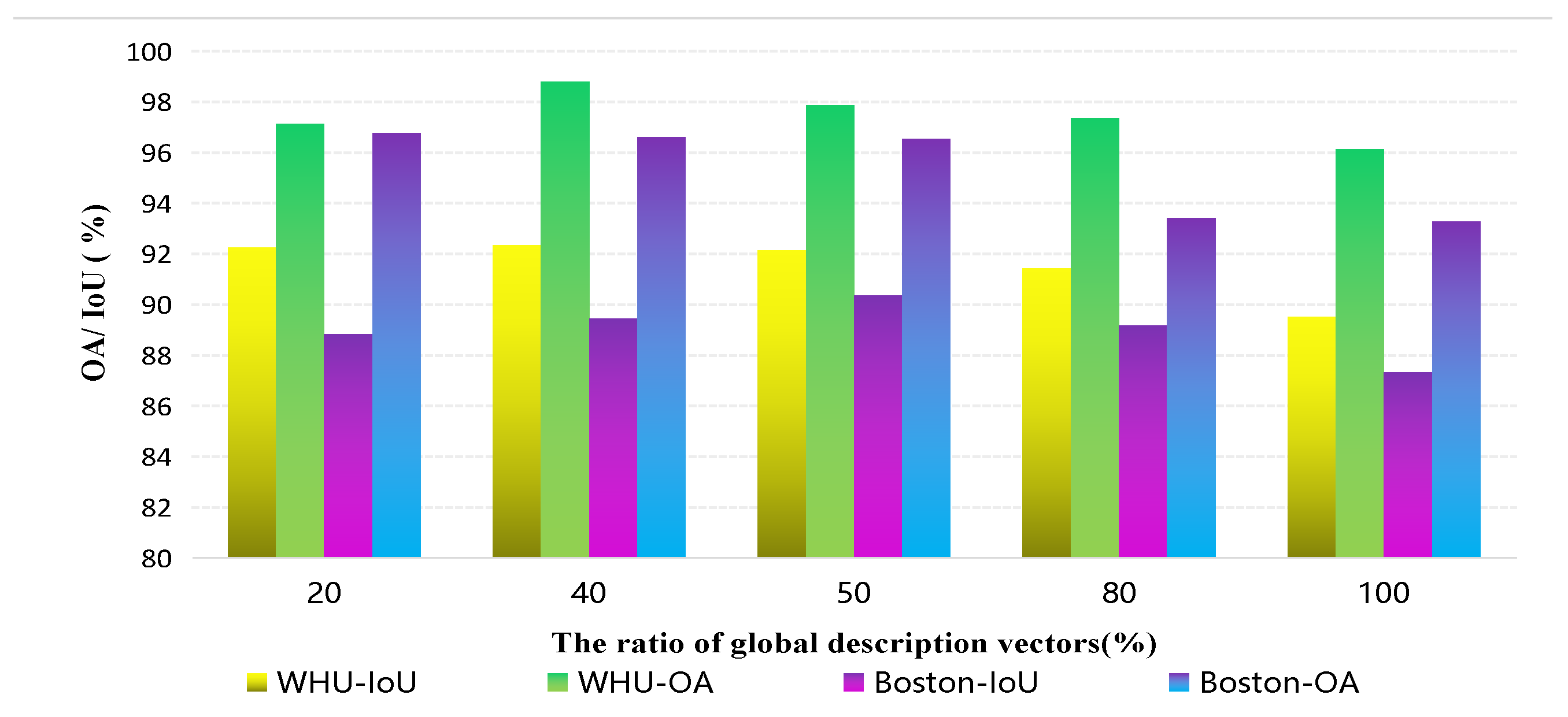
3.2.2. Global Context Description Vectors

In principle, the MCOM aims to generate various contextual descriptions for global information interpretation. Global context description vectors are the important component of the module, which recalibrate feature maps to calculate the context information from different regions. As shown in Figure 2, the MCOM makes the aggregation of information from high and low feature maps by Gj(·) in the Equation (3). Each block in the context pyramid consists of two branches. The first branch calculates the feature weight coefficients of all subregions, while the second branch recalibrates features of subregions to encode corresponding global information. Details are described as follows.
First, to generate global context encoders and reduce the computational complexity, Xl and Xh are linearly transformed into features xl and xh by 1 × 1 convolution in Equation (4), the channels of which are reduced by C/r and g (r is the rate of channel reduction), respectively. Then, they are both transmitted into the spatial pyramid pooling (SPP) [26] model in a parallel way to obtain multiscale representations. The above process can be expressed as Equation (2), where fsu and fsl are the feature maps in scale s and p o o l i n g denotes down-sampling operation with pooling layers. Generated feature maps are normalized by the softmax function. Overall, Gsi∈Gs represents the i-th unique semantic code in the s scale. It can be calculated as Equation (3), where (v,w) and (n,m) represent an arbitrary position on fsl and fsu, respectively. This operation aggregates context in spatial locations using across-level features and can adaptively construct global information for the network. Meanwhile, the whole spatial features of fsl can be retained in each channel-wise. The contextual description vectors are built, capturing global information in different aspects. Finally, global context descriptions are concatenated into a vector of semantic representations Gs in scale s, which provides rich global information guided by high-level features for Xl.
f s u = p o o l i n g ( x h ) , f s l = p o o l i n g ( x l )
G s i = j s i 2 e x p ( f s u ( v , w ) ) n , m e x p ( f s u ( n , m ) ) f s l ( v , w )
x l = φ i ( X l ) = w 1 X l , x l = ψ j ( X h ) = w 2 X l

3.2.3. Multiscale Global Context Pyramid

After transformation via SPP and Gs for Xl and Xu, a global context pyramid architecture can be constructed, where each block can encode the global semantic feature at different scales. Furthermore, we concatenate these semantic codes and global average pooling of xh along the channel dimension, which finally generates a global semantic coding map GP P × C / r   (P = g × s) in Figure 2. Then, Xl is transformed to xl H × W × P by 1 × 1 convolution, and multiscale global context can be obtained by matrix multiplication with xl and GP. To fuse local and global features, global context is added to xl using the skip-connection in the network. Finally, combining with Equations (1)–(4), enhanced feature Z can be obtained as Equation (5), where concat(·) denotes concatenation operation and GAP denotes global average pooling.
Z ( X l ) = w 2 X l + s = s 1 p w 1 X l c o n c a t ( G P , GAP ( x h ) )

3.3. Semantic Guided Spatial Attention Module

Although the deep-level feature map has rich semantic information, it lacks spatial detail information. The common method is upsampling deep level maps and fusing the low-level feature using skip-connection to restore fine-grained structural details, especially the boundaries of buildings. However, on the one hand, across-level feature fusion probably causes information redundancy without refinement. On the other hand, different hierarchical features adopt local operations such as bilinear interpolation or deconvolution to increase resolution in upsampling. However, this method ignores long-range spatial interdependence for each pixel in global features. To address this problem, many attention models simulate semantic interdependence in spatial or channel dimensions, such as DANet and SEnet. However, these attention mechanisms often come from the same encoder layer and ignore the semantic gap and dependence relationship between across-level features. Deep-level features have large receptive fields containing rich semantic features to guide the filtering for shallow features. Therefore, to alleviate the semantic gap of different scale features, inspired by non-local networks [36] and CBAM [34], we designed a spatial attention module to recover the building’s fine-grained features and optimize the decoder in shallow layers.
First, we construct a similarity matrix using the high-level and low-level feature maps to capture a wide range of position dependence. As illustrated in Figure 3, a shallow layer feature Xl H1×W1×C1 and a deep layer feature Xh H2×W2×C2 are transmitted into 1 × 1 convolution layers to generate two new feature maps fl and fh, respectively, in Equation (6), where fl H1×W1×C and fh H2×W2×C. Then, they are reshaped into M×C, N×C, respectively, where M = H1 × W1 and N = H2 × W2. A similarity matrix F can be obtained by a matrix multiplication with fl and fh, F M×N in Equation (7). Therefore, we can calculate average pooling and maximum pooling along N dimension of F to aggregate feature in all position on M dimension, respectively, and then reshape it into F H1×W1×2, where F is the new feature map with two channels.
f l = c o n v ( X l ) , f h = c o n v ( X h )
F = f l ( f h ) T
α ( F ) = σ ( c o n v ( A v g P o o l ( F ) © M a x P o o l ( F ) ) )
A spatial attention map α ( ) that integrates the features F can be described via in Equation (8), where conv(·) denotes convolution operation; AvgPool(·) and MaxPool(·) denote average pooling and maximum pooling operations, respectively; © presents the concatenation operator; and σ (·) denotes the softmax function. In this paper, we use a convolution 7 × 7 to fuse feature maps with two channels. Finally, shallow feature Xl from the encoder is converted into a new feature map Xl by matrix multiplication with α ( ) .
X l = α ( F ) × f l

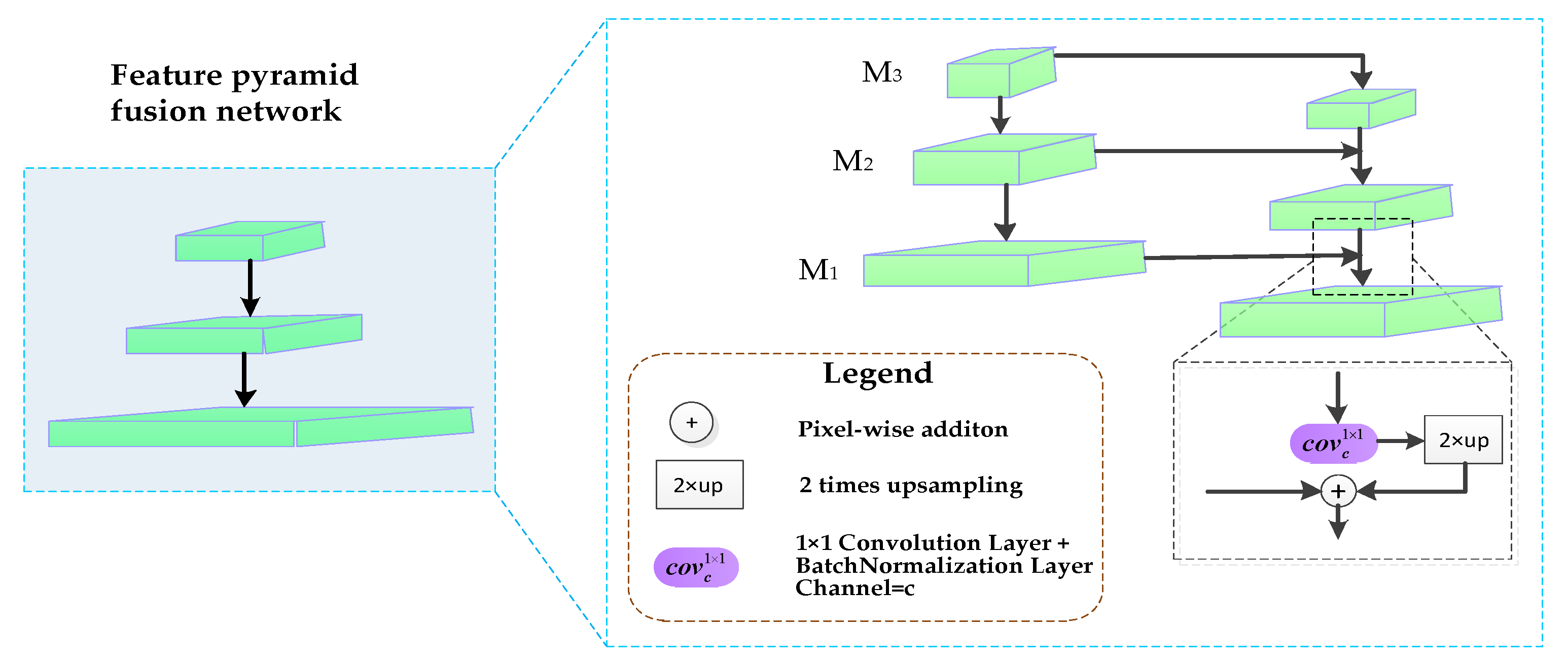
3.4. Feature Pyramid Fusion Network

The feature pyramid network is an effective structure to fuse multiscale features, which are usually used for target detection. Currently, it has been used for semantic segmentation or panoramic segmentation [40] and achieved excellent results. We construct a feature pyramid structure to fuse different level features and achieve accurate prediction. The top-down pathway is built with skip-connection, as illustrated in Figure 1. In the backbone network, middle-level and high-level feature maps from the encoder of residual block3 and block4 are converted into F4 and F5 via MCOM. Owing to their shared spatial resolution, we can obtain a fused feature M3 by pixel-wise addition using F4 and F5. Hence, M3 fused local features and multiscale global context, which assists the network to refine coarse features and guide upsampling operations. M3 and features from residual block2 or block3 are simultaneously fed into the SAM, and M1, M2 can be obtained. Finally, M1, M2, and M3 are fused by pixel-wise addition and upsampling to progressively increase the spatial resolution, generating the final predicted map as shown in Figure 4.

4. Experiment Design

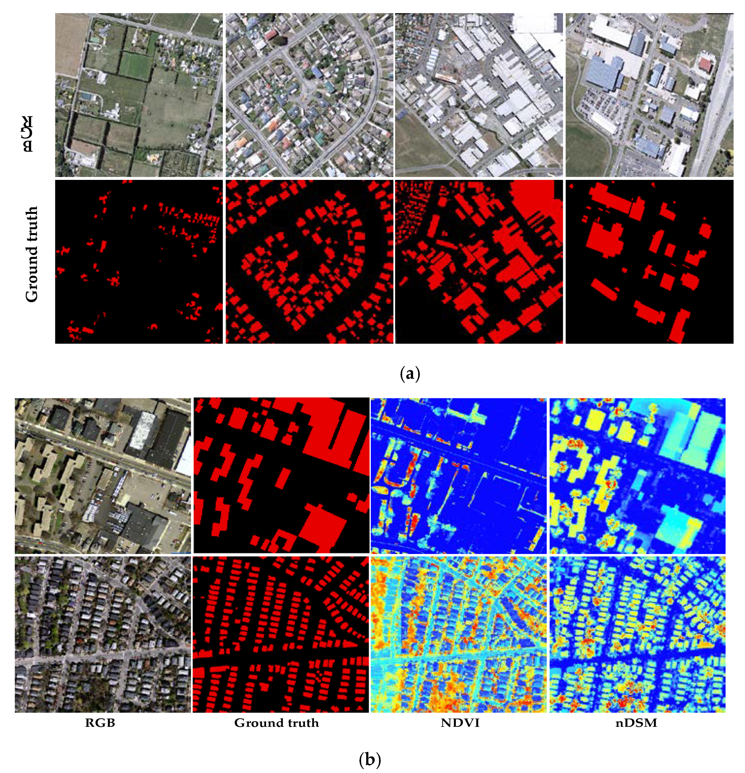
4.1. Dataset Description

In order to test the effectiveness of the algorithm in three sections, two types of public datasets are used in the experiment. One is the WHU building dataset [41] with the high-resolution aerial orthophotos, and the other is the Boston building dataset using the multi-modal remote sensing data. For the former, aerial images, including R (red), G (green), and B (blue) bands with 0.075 m spatial resolution, cover 450 km2 in Christchurch, New Zealand, and have more than 220,000 independent buildings. The dataset also provides manually edited labels of buildings for training and evaluating algorithms.
For the Boston building dataset, we collected multispectral high-resolution aerial orthoimages with 0.3 m spatial resolution that can be obtained from the United States Geological Survey (USGS) [42]. This dataset consists of eight orthoimages with four bands, including R, G, B, and near-infrared (NIR), and covering about 18 km2 in Boston, MA, USA. The whole imageries were processed to correct lens distortion, remove clouds, and make images color-uniform. Meanwhile, LiDAR point cloud data with 0.35 m estimated point spacing, 5.2 m vertical accuracy, and 0.36 m horizontal accuracy were obtained from NOAA for Coastal Management [43]. The shapefiles of building footprints can be downloaded from the Massachusetts buildings dataset [44] and open street maps (OSM).
The two datasets represent buildings with different densities, variable sizes, and a variety of shapes in the complex background environment, which ensures the robustness of the algorithm and the prediction ability of multi-modal data fusion. As shown in Figure 5, many buildings are covered by vegetation and shadows and some roads and buildings have similar texture features, bringing some challenges to building extraction. In the urban area, the density and height of buildings are greater than that in the suburb. In addition, to analyze the robustness of the algorithm for the large-scale buildings and the regions with uneven density distribution, we selected two typical areas from the test dataset to analyze and compare with other deep convolutional models.

4.2. Data Preprocessing

In Table 1, the relevant information of the dataset is listed for model testing and training, including the data type, image resolution, data acquisition time, and location. For the WHU building dataset, 60% area of the whole aerial image as a data subset is used and downsampled into 0.15 m spatial resolution with cropping into 9827 tiles with 512 × 512 pixels. The cross-validation dataset was established, including the training dataset, validation dataset, and test dataset, which contains 70,456 buildings, 8562 buildings, and 24,674 buildings, respectively. Correspondingly, vector files of building footprints have been manually edited, referring to the original aerial image, are also rasterized to the same spatial resolution.
The Boston dataset contains multi-modal data, including multispectral imagery and LiDAR dataset. First, due to polygons of OSM derived from different times, we correct its errors and compensate the missing building footprints referring to the original aerial orthoimages and labels of the Massachusetts buildings dataset to generate accurate labels. Polygon labels are rasterized into 0.3 m spatial resolution label images. Second, outliers and noise points are removed from LIDAR point cloud data using CloudCompare software [45]. The unclassified clean LiDAR data and ground LiDAR point cloud data are interpolated using the Kriging interpolation algorithm to generate the digital surface model (DSM) and the digital elevation model (DEM).
Finally, to distinguish the bare-ground, road, and buildings, the normalized DSM (nDSM) image as a band data contain the height information of the object through the difference of DSM and DEM. For feature extraction and training, nDSM image is also processed to the same spatial resolution as orthoimages. For multispectral images, the NDVI image is calculated using the R band and NIR band. All data are integrated into the image format with multiple channels and cropped into 512 × 512 pixels tiles with the overlap of 512 pixels for training and testing on network models.
Because Boston data training samples are insufficient for training a large number of parameters, data enhancement methods are used to increase training samples and improve the model’s generalization ability. All training samples are rotated by 90°, mirrored in the horizontal and vertical directions, and random noise is added to 10% of the dataset. Finally, the enhanced dataset and original data as inputs are used to train the model.

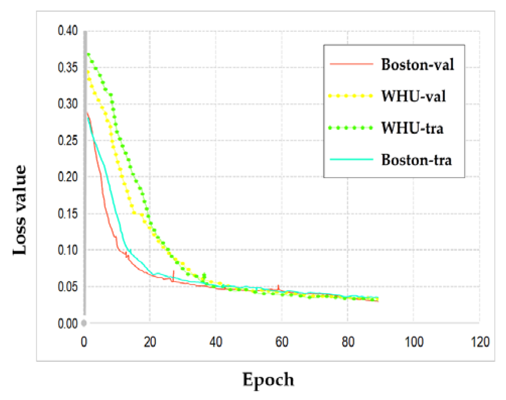
4.3. Experimental Setting

Our model was implemented using the Keras framework with Tensorflow backbend on the GeForce RTX 2070 GPU. The network was trained using Adam’s optimization algorithm by minimizing the cross-entropy losses with the initial learning rate of 0.001, weight decay of 0.0001, momentum of 0.9, and batch size of 6. The backbone network is initialized using the pre-trained weight parameters of ResNet-50, while other parameters were initialized using Xavier’s [46] method. When the training loss value decreases, but validation dataset loss value remains unchanged or increases in four consecutive iterations, the learning rate will decrease with the attenuation ratio of 0.15. The model stops training when the validation dataset loss does not change within 10 consecutive iterations. The loss value of the WHU and Boston datasets with the increasing epochs are shown in Figure 6.
In the WHU building dataset, the R-G-B composite images were fed into the different networks, while R-G-B-NDVI and nDSM as multi-modal images were fed into networks in the Boston subset. Two branches of networks were adopted for the in Fused-FCN4s, where R-G-B-NDVI and nDSM were fed into two sub-networks, respectively. The comparative model configuration is the same as the proposed model without postprocessing.

4.4. Accuracy Assessment

Three commonly used accuracy matrices, including the overall accuracy, mean intersection over union, and F1-score, are used to evaluate the performance of the method in the semantic segmentation task. OA is the ratio of correctly predicted pixels to the total pixels, and IoU describes the statistical relationship between the set of ground truth and predicted segmentation as follows:
O A = T P + T N T P + F N + F P + T N
I o U = T P F N + F P + T P
where TP (true positive) is the number of pixels that the prediction and the corresponding ground true are all positive; TN (true negative) is the number of pixels that the prediction and the corresponding ground true are all negative; FP (false positive) is the number of pixels that prediction result is positive, while the corresponding ground true is negative; and FN (false negative) is the number of pixels that prediction result is negative, while the corresponding ground true is positive. We can calculate precision and recall in Equation (12) with TP, FP, and FN. In addition, F1-score is defined in Equation (13) to measure the accuracy of the binary classification model in statistics.
P r e c i s i o n = T P T P + F P , R e c a l l = T P T P + F N
F 1 - s c o r e = 2 P r e c i s i o n × R e c a l l P r e c i s i o n + R e c a l l

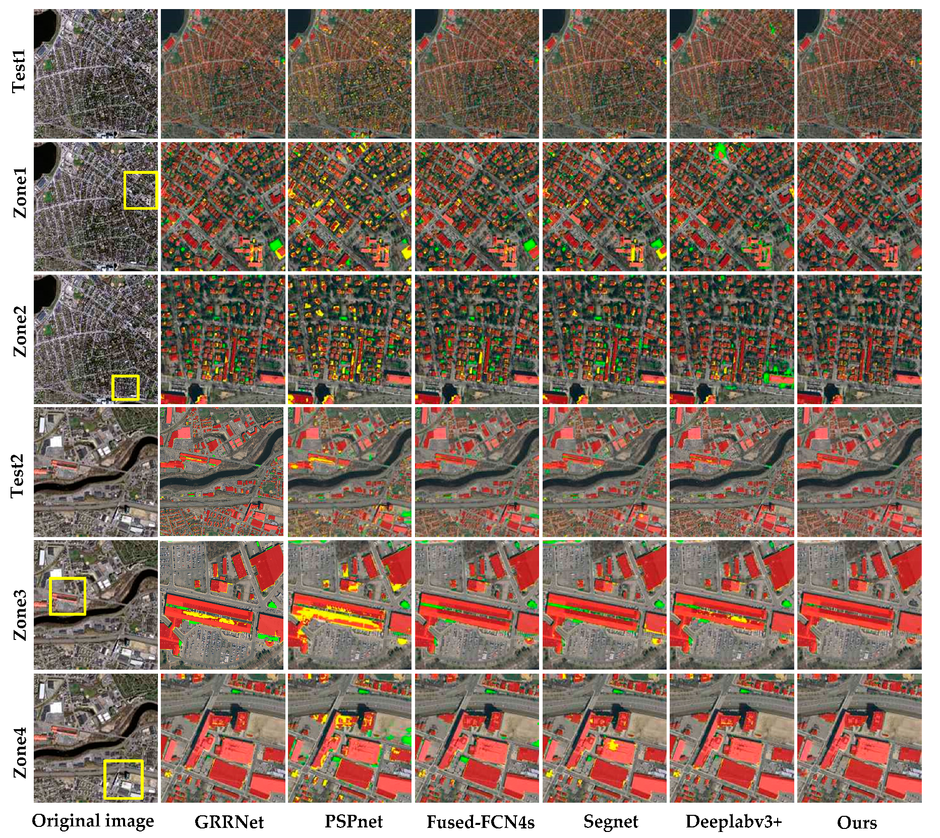
5. Experiment Results and Analysis

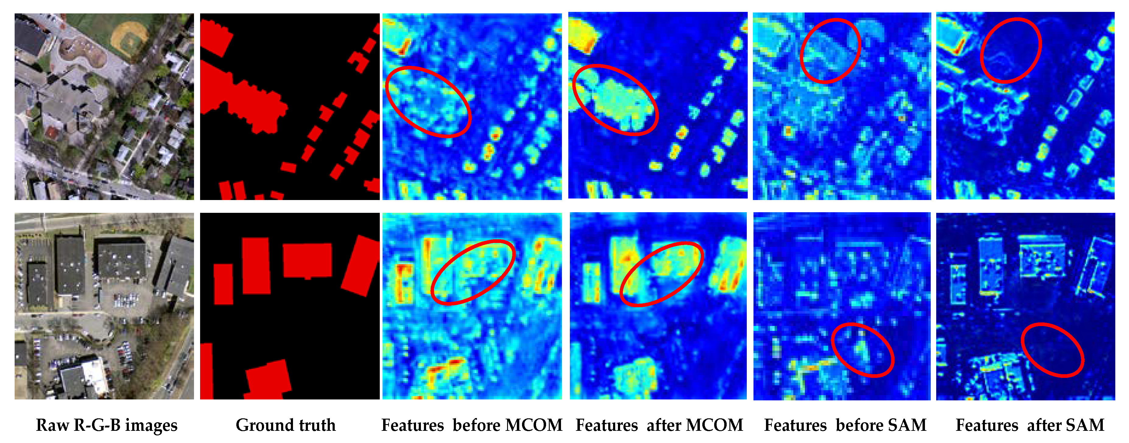
5.1. Ablation Experiments

An ablation experiment was conducted on the WHU dataset and the Boston dataset with accuracy metrics including OA and IoU to evaluate quantitative performance. The same experiment condition is set to compare the performance of building extraction with different parameters. The feature from different modules and encoder layers are fused by FPN architecture using skip-connection. In this work, we use two patterns to train the model for suiting different data types. As shown in the decoder parts of Figure 1, the network uses pattern A (backbone + branch + decoder) to extract features for multi-modal data, while pattern B (backbone + decoder) extracts features for multispectral data. WHU data are used for pattern A due to only containing RGB bands, and the experimental results are shown in the following sections. In Section 5.1.3, we only use the Boston dataset to explore the impact of multi-modal data on building extraction.

5.1.1. Ablation on Multiscale Global Context Module

To evaluate the effectiveness of the MCOM, we set different hyperparameters, including various pooling rates, types, and the number of global description vectors GS in comparable experiments. MCOM is followed by residual block3 and block3, and SAM is removed. Specifically, four sets of different pooling rates, 2/3/6, 2/4/8, 3/6/8, and 3/4/8, are applied in modules, and the number of global description vectors is initially set to 50% of the feature channel numbers. In addition, the global average pooling is the branch for the module when using different pooling rates. Max and average pooling were used to generate comparative results for testing the proposed method.
Pooling rates: In the experiment, the pooling size will influence the performance of the result, as shown in Table 2. We choose the different pooling sizes from small to large to capture the feature from various scale local regions. It is reported that the rates of 2/4/8 and global average pooling get the best results that outperform other settings. Thus, they are adopted in the proposed module.
Pooling types: The statistical result on two datasets displayed that using average pooling is more around OA of 0.02–0.5% than using max pooling. Therefore, we use average pooling in experiments.
Global description vectors: As listed in Figure 7, the number of global description vectors has an impact on the accuracy of results, where it is set ranging from 20% to 100% of the feature channel numbers. It is observed that IoU and OA increased the WHU dataset and the Boston dataset between 20–40%. However, the accuracy metrics dropped gradually, especially when the number of global description vectors is over 40%, which is probably caused by the increase in computation and parameters that will lead to overfitting. Moreover, the large size feature maps can significantly increase the computational cost. Therefore, to leverage efficiency and accuracy for the model training, the number of global description vectors is determinate as 30% of the feature channel numbers.
Figure 8 shows the heat map of spatial regions response before and after feature transformation via MCOM or SAM. We calculate the average fused feature from residual block3 and block4 in the channel dimension. Obviously, compared with the third and fourth columns, most of the background-related information is suppressed after MCOM. In addition, the large-scale building area has a more significant holistic response than the previous local attention, as shown in the red ellipse.

5.1.2. Ablation on Spatial Attention Decoder

In this section, the spatial attention decoder was tested to evaluate the influence for the model without the branch of MCOM. In Figure 1, the middle-level and high-level features (F3 and F4) are transmitted as the attention map to refine the feature of the encoder from low-level layers. Table 2 reported that IoU increased by about 2.37% in the WHU dataset and 2.64% in the Boston dataset. Compared with the fifth and sixth columns in Figure 9, the boundary features of buildings have a strong response via SAM, and the features of classification ambiguity have been corrected, as shown in the red ellipse.

5.1.3. Ablation on Different Data Inputs

Different data types in the Boston dataset as input were divided into different data groups to verify the effectiveness of the model. Table 3 lists the impact on classification results employed for two network patterns for different data input combinations, where RGB, NIR, and NDVI as spectral images were fed into backbone network using pattern A, while nDSM as unique input was fed into the branch network using pattern B. Compared with using spectral image alone, the fusion of the nDSM feature can help the backbone network increase by approximately 2.5% of OA and 3.7% of IoU, which implies that LiDAR data can significantly improve the classification accuracy. Using the “RGB+NDVI” as input for the backbone network slightly improves the performance over “RGB+NIR”, while the OA and mIoU increased by approximately 1.2% and 0.7%, respectively, compared to using “RGB” alone. The combination of “RGB+NDVI” with nDSM obtained a better result than other data groups, which indicates that the fusion of spectral features with the elevation of LiDAR can further improve the results for building extraction.

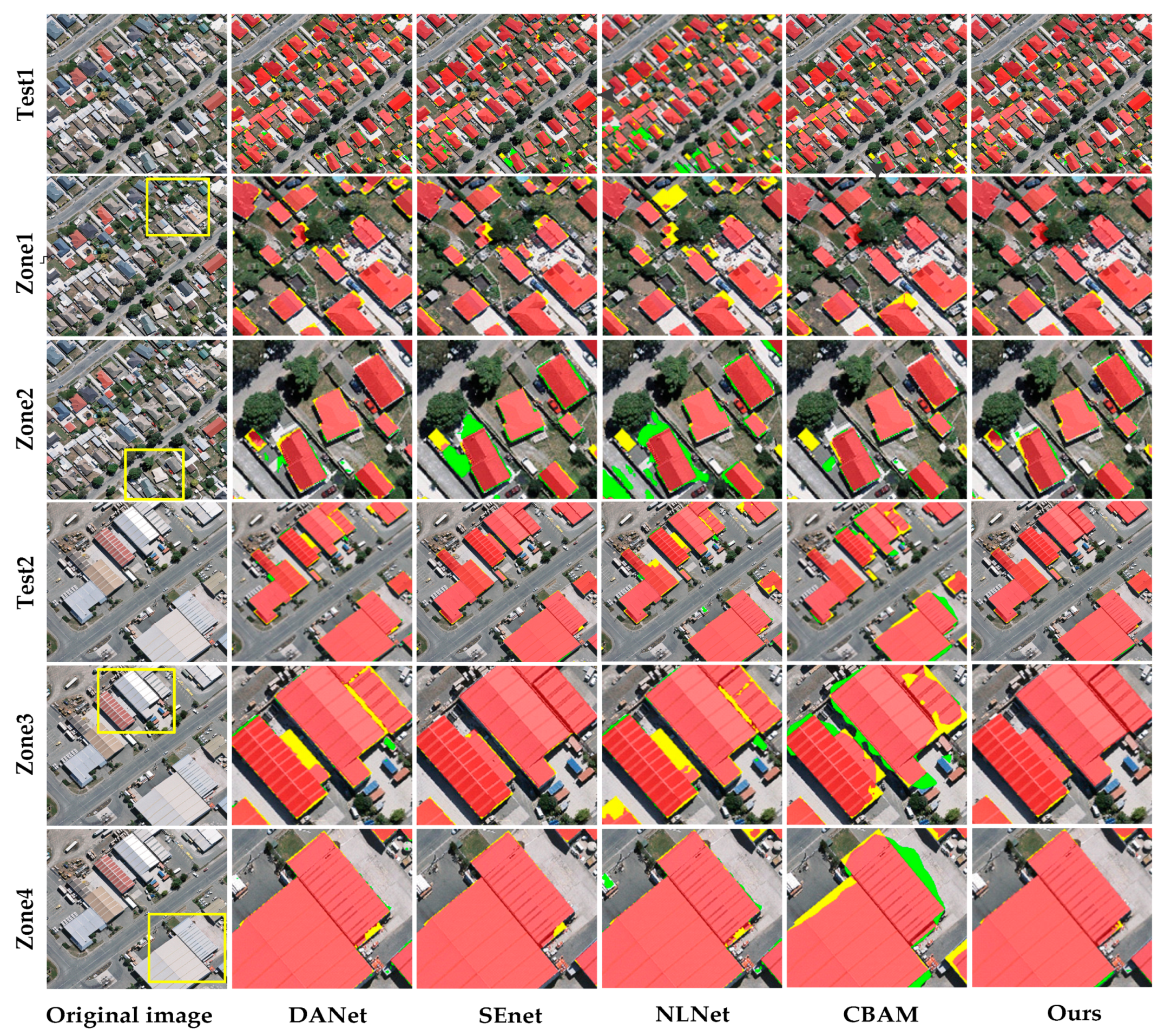
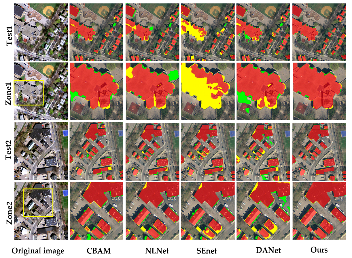
5.2. Comparison of Attention Mechanism

The performance of building extraction is exhibited in Figure 8 using different attention modules. Closer inspection marked in yellow rectangles can be viewed in rows 2, 3, 5, and 6. The model adopts the same FCNs framework (backbone network + attention modules) with FPN and substitutes for SAM and MCOM to fuse and generate the results using different attention mechanisms.
In WHU, our networks outperform other attention modules, implying that the combination of multiple global context attention and spatial attention modules can effectively improve the result of multiple-scale building extraction. SEnet could identify most buildings, but in detail, it struggled with boundaries and corners of the building in zone 1 and zone 2. Although DANet and CBAM network obtain a better result than SEnet in test1, pixels are misclassified in zone 3 and zone 4. This result indicates that spatial attention and channel attention can enhance the ability to filter features with the tragedy of multi-level feature fusion, but for the varied scale and the large regions of buildings, they have a weak ability to integrate different scale features. Compared with other models, NLNet did not perform well due to many FNs in test1. As only using global spatial attention is effective for long-range dependencies, it neglects the influence of the dependence between channels.
Figure 10 exhibits the result of building segmentation for the Boston dataset. Visually, our model and CBAM obtained better global results than other modules. As shown in the close-ups of rows 2 and 4, compared to CBAM, our model not only achieved better performance in the boundaries of buildings but can capture different scale receptive information with fewer FPs for the large scale area. NLNet has a relatively well result in the sparsely distributed build-up in zone 2, while it tended to misclassify pixels in the area covered by shadows and roads in zone 1. For DANet and SKnet, many FPs and FNs existed in zone 1, where it is difficult for them to identify large building areas.
Table 4 also illustrates the statistical accuracy metrics obtained through classification. The current result of the proposed method has superior performance over other mentioned models with the OA, IoU, and F1-score on the datasets. DANet also obtained accurate results with high OA, but it performs poor results in WHU dataset with an IoU 9.6% lower and an F1-score 4.8% lower than our method. Meanwhile, it can be observed that DANet and CBAM outperform SKnet and NLNet in the WHU dataset with high IoU and F1-score in the Boston dataset, which further proved that the integration of channel and spatial attention could effectively improve the accuracy of building segmentation. With auxiliary from feature pyramid network (FPN) and new modules, the backbone network can significantly improve the OA and IoU by almost 4% and 6% in Table 2. Obviously, that result manifests that an attention mechanism combining the FPN architecture can enhance the multiscale feature fusion and increase the accuracy of segmentation. Therefore, a well-versed feature extraction strategy using our proposed modules is suitable for multiple-scale building extraction.

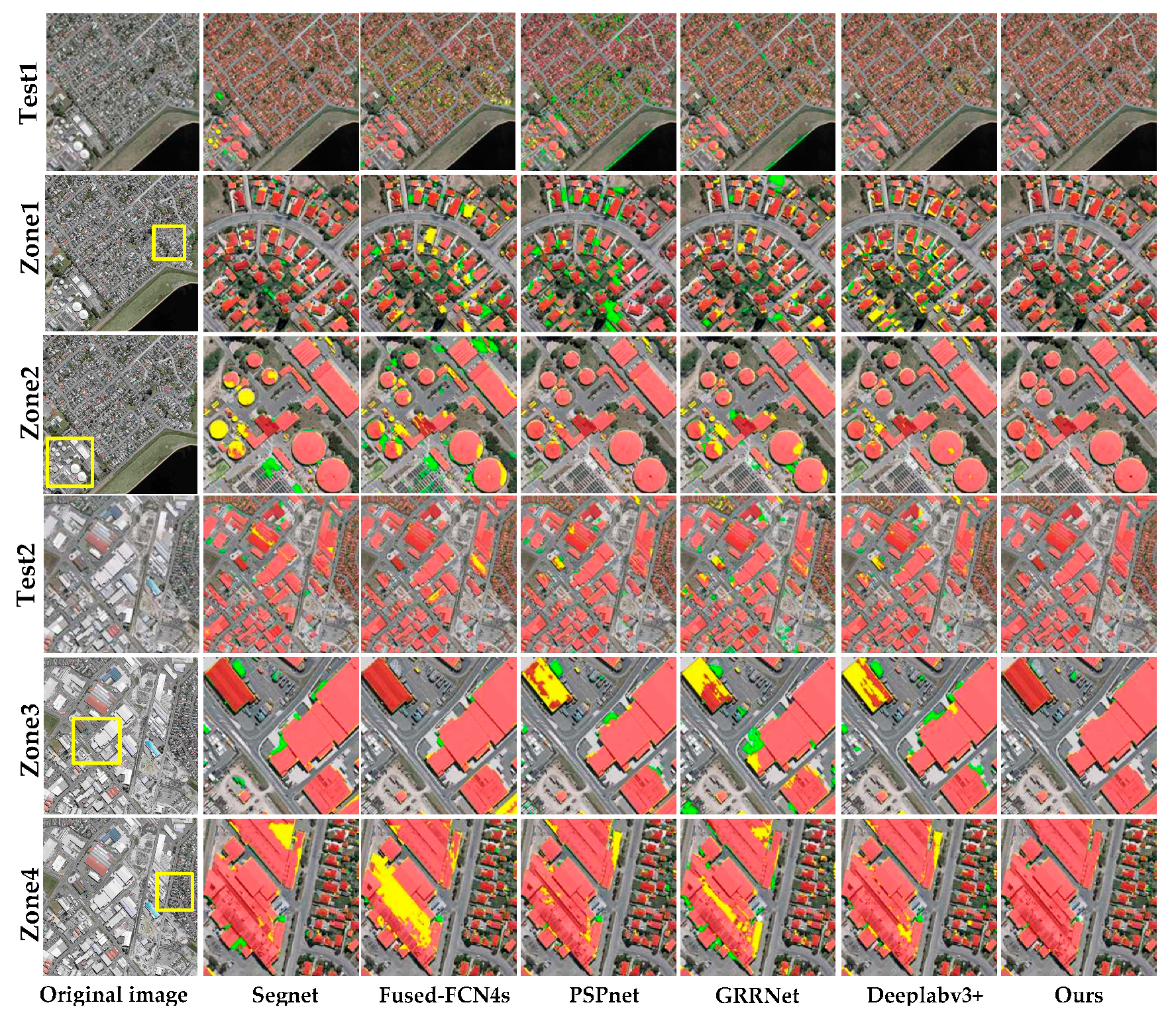
5.3. The Proposed Model with Different Network Frameworks

We selected five representative FCN models for comparison in the experiment: Fused-FCN4s [24], SegNet [28], PSPNet [26], GRRNet [22], and Deeplabv3+ [27]. These methods are easy to complete with open source code. Figure 11 presents the classification results of different full convolution models in the WHU building dataset with only input of R, G, and B bands of high-resolution aerial images and the close-ups (as marked in yellow rectangles) for the detailed extraction results.
In the test dataset, two sub-areas with uneven distributions of area and density are used for comparison and analysis. Our method and Deeplabv3 + obtain better classification performance through visual observation than other models in the densely distributed and large-area building area. However, Deeplabv3 + did not achieve excellent performance in WHU zone 4 as large-scale building blocks appeared as some undetected pixels. Although the ASPP module enhances multiscale receptive field information, they are given the same weight and lack globally multiscale semantic information. In contrast, the MCOM can aggregate global semantic features and has good segmentation results in large-scale building areas. PSPnet has relatively good extraction results in zone 2 and zone 4, while there are many FNs and FPs in zone 1 and zone 3, where roads are easily misclassified as buildings, implying that the pyramid pooling model can capture context features of multiple scales, but it has inferior extraction ability in small and dense building areas.
Visually, SegNet delivered relatively good segmentation results in zone 1 and zone 3. However, in some local areas, such as bare land and roads, many pixels are misclassified as buildings, and there are many discontinuous extraction results in the local region of zone 2 and zone 4. As a result, although maximum pooling index technology and multiscale feature fusion method of SegNet can improve feature extraction, they are not filtered and selected, which will negatively impact the segmentation results. Fused-FCN4s and GRRNet obtained better classification results in relatively uniform scale areas of buildings than multiscale building areas in urban areas. In zone 1 and zone 2, many FNs can be found in the area shaded by shadows and around trees. Moreover, the segment results of zone 4 display that many building pixels are not detected, which indicates that Fused-FCN4s and GRRNet have a weak ability to extract large-scale building blocks.
Figure 12 exhibits the results of building extraction using the Boston dataset for different methods. Our models outperform other models in the prediction of urban regions, and only a small amount of FPs are presented, which indicates that the proposed modules combining with multi-modal data can improve the result of building extraction. Fused-FCN4s and GRRNet achieve good performance, but there are still a number of FNs in large-scale building regions and boundaries. Deeplabv3+ obtained better results for buildings of a suburb than Fused-FCN4s and GRRNet, but in the dense urban area, it is sensitive to the features of cars and roads with a similar texture and spectral reflectance with rooftops, so which of these pixels are misclassified as a building. Similarly, PSPNet generally exhibits better performance than Deeplabv3+ and Fused-FCN4s in the suburbs but still frequently misclassified road and plantation pixels as building pixels in the urban area.
Accuracy evaluation in Table 5 is summarized for quantitative analysis and comparison of different convolutional neural networks. Our networks achieved the best outcome with OA, mIoU, and F1-score among the two public datasets. Although Deeplabv3+ has a relatively high OA of 97.55% in the WHU building dataset, the mIoU is 3% lower than that of our model. GRRNet and Fused-FCN4s achieved relatively high IoU and F-1 scores in Boston, but do not perform well in the WHU dataset. PSPnet has comparable results with Deeplabv3+ in the Boston dataset, but the result only obtained an IoU of 73.87% and an 85.73% F-1 score in the WHU dataset. The results imply that the pyramid pooling strategy cannot effectively recover the detailed feature information.

6. Discussions

Using a multiscale context optimization module and spatial attention module, the proposed model achieves excellent performance for building extraction. The experimental results also confirm that the segmentation accuracy of the model for building can be improved by fusing the features of LiDAR data and the spectral information from high-resolution aerial images.
In MCOM, semantic descriptors apply a pyramid pooling strategy to obtain multiscale global semantic information. Different from other multiscale context models, the proposed MCOM can simultaneously capture the spatial interdependence of multiple regions and assemble global context information through various semantic encoders for each channel. The proposed SAM selectively focuses on effective information and suppresses useless features. To leverage the efficiency of hierarchical feature fusion, MCOM is applied to deeper layers features due to rich semantic information, while a SAM is used in shallow layers with high resolution in details.
The proposed model could be further improved with the following research aspects. First, the appropriate number of global semantic descriptors is obtained by experiments in the MCOM. For different datasets, this parameter probably needs to be reset to achieve the optimized global context information. As a result, it is necessary to take adaptive parameters for different datasets. Second, the model only uses high-resolution images and LiDAR data. It is necessary to establish the combination with other resources such as hyperspectral imagery. In addition, the error from nDSM interpolation and registration between LiDAR and raw images will have a negative impact on the result. The 3D spatial information of LIDAR point clouds can provide essential clues for building feature detection. Hence, the network framework could be designed to integrate 3D and 2D information. Although the model improves the accuracy of building extraction, the large amount of parameters lead to a decrease in computation cost as shown in Appendix A. In the future, we still need to improve the efficiency of the model. In the model structure, we did not explore the impact of multi-branch networks and backbone networks on the results. For multiple modal data, using shared or non-shared parameters may affect the results.

7. Conclusions

In this paper, a novel, fully convolution network framework is presented for building extraction in complex remote sensing scenarios. The major contribution of the study is to optimize and effectively fuse multiscale features from multi-modal data to improve the performance of building segmentation. The modified end-to-end residual FCNs architecture is applied for feature extraction using the high-resolution airborne imagery or the combination with LiDAR data. The proposed multiscale context optimization module (MCOM) can learn semantic representations from multiscale subregions and generate more discriminative features by constructing global semantic correlations and adaptively aggregating local context information. A semantic guided spatial attention mechanism is designed to relieve the semantic feature gap between encoders and refine shallow features by constructing across-level feature independence. Compared with other classic approaches, our experimental evaluation results on two types of public datasets demonstrated that the proposed model achieved competitive performance for multiple-scale building extraction.

Author Contributions

Q.Y. wrote the paper and completed experiments; H.Z.M.S., A.H.A., and S.J.b.H. supervised the study and reviewed the paper. All authors have read and agreed to the published version of the manuscript.

Funding

This work was supported by the Youth Science Foundation of Panzhihua University under grant no. bkqj2020024.

Data Availability Statement

WHU building Dataset can be obtained via file:///F:/Wuhanbuilding_extraction_data/Description%20of%20the%20WHU%20Building%20Dataset.html (accessed on 10 May 2021). Boston image and LiDAR dataset can be downloaded via https://earthexplorer.usgs.gov/ (accessed on 10 May 2021); https://coast.noaa.gov/dataviewer/(accessed on 10 May 2021). Vector files of Boston building footprints can be obtained via https://www.cs.toronto.edu/~vmnih/data/mass_buildings/massachusetts_buildings_shape.zip (accessed on 10 May 2021).

Acknowledgments

The authors would like to thank all the colleagues for the fruitful discussions on this work. The authors also sincerely thank the anonymous reviewers for their very competent comments and helpful suggestions.

Conflicts of Interest

All authors declare no conflict of interest.

Appendix A

Table A1. Complexity comparison with other modules.
ModelWHU DatsetBoston Datset
Parameter Size (MB)GFLOPsParameter Size (MB)GFLOPs
SegNet112.332.64127.82.34
GRRNet100.344.57116.53.35
Senet95.743.87105.672.77
DANet119.762.37134.383.47
CBAM127.633.64133.792.37
NLNet137.842.45157.362.87
PSPnet178.841.28217.351.78
Deeplabv3+158.395.32167.874.62
Fused-FCN4s93.142.79100.22.14
Ours138.474.73148.963.72

References

  1. Jin, X.; Davis, C.H. Automated building extraction from high-resolution satellite imagery in urban areas using structural, contextual, and spectral information. EURASIP J. Adv. Signal Process. 2005, 2005, 745309. [Google Scholar] [CrossRef] [Green Version]
  2. Huang, X.; Zhang, L. Morphological Building/Shadow Index for Building Extraction from High-Resolution Imagery over Urban Areas. IEEE J. Sel. Top. Appl. Earth Obs. Remote Sens. 2012, 5, 161–172. [Google Scholar] [CrossRef]
  3. Pesaresi, M.; Gerhardinger, A.; Kayitakire, F. A robust built-up area presence index by anisotropic rotation-invariant textural measure. IEEE J. Sel. Top. Appl. Earth Obs. Remote Sens. 2008, 1, 180–192. [Google Scholar] [CrossRef]
  4. Ghanea, M.; Moallem, P.; Momeni, M. Automatic building extraction in dense urban areas through geoeye multispectral imagery. Int. J. Remote Sens. 2014, 35, 5094–5119. [Google Scholar] [CrossRef]
  5. Tang, Y.; Li, L.; Wang, C.; Chen, M.; Feng, W.; Zou, X.; Huang, K. Real-time detection of surface deformation and strain in recycled aggregate concrete-filled steel tubular columns via four-ocular vision. Robot. Comput.-Integr. Manuf. 2019, 59, 36–46. [Google Scholar] [CrossRef]
  6. Tang, Y.C.; Wang, C.; Luo, L.; Zou, X. Recognition and localization methods for vision-based fruit picking robots: A review. Front. Plant Sci. 2020, 11, 510. [Google Scholar] [CrossRef] [PubMed]
  7. Gharibbafghi, Z.; Tian, J.; Reinartz, P. Modified super-pixel segmentation for digital surface model refinement and building extraction from satellite stereo imagery. Remote Sens. 2018, 10, 1824. [Google Scholar] [CrossRef] [Green Version]
  8. Sirmacek, B.; Unsalan, C. A probabilistic framework to detect buildings in aerial and satellite images. IEEE Trans. Geosci. Remote Sens. 2010, 49, 211–221. [Google Scholar] [CrossRef] [Green Version]
  9. Liasis, G.; Stavrou, S. Building extraction in satellite images using active contours and color features. Int. J. Remote Sens. 2016, 37, 1127–1153. [Google Scholar] [CrossRef]
  10. Mongus, D.; Lukač, N.; Žalik, B. Ground and building extraction from LiDAR data based on differential morphological profiles and locally fitted surfaces. ISPRS J. Photogramm. Remote Sens. 2014, 93, 145–156. [Google Scholar] [CrossRef]
  11. Du, S.; Zhang, Y.; Zou, Z.; Xu, S.; He, X.; Chen, S. Automatic building extraction from LiDAR data fusion of point and grid-based features. ISPRS J. Photogramm. Remote Sens. 2017, 130, 294–307. [Google Scholar] [CrossRef]
  12. Huang, R.; Yang, B.; Liang, F.; Dai, W.; Li, J.; Tian, M.; Xu, W. A top-down strategy for buildings extraction from complex urban scenes using airborne LiDAR point clouds. Infrared Phys. Technol. 2018, 92, 203–218. [Google Scholar] [CrossRef]
  13. Xia, S.; Wang, R. Extraction of residential building instances in suburban areas from mobile LiDAR data. ISPRS J. Photogramm. Remote Sens. 2018, 144, 453–468. [Google Scholar] [CrossRef]
  14. Lai, X.; Yang, J.; Li, Y.; Wang, M. A building extraction approach based on the fusion of LiDAR point cloud and elevation map texture features. Remote Sens. 2019, 14, 1636. [Google Scholar] [CrossRef] [Green Version]
  15. Tang, Y.; Chen, M.; Lin, Y.; Huang, X.; Huang, K.; He, Y.; Li, L. Vision-Based Three-Dimensional Reconstruction and Monitoring of Large-Scale Steel Tubular Structures. Adv. Civ. Eng. 2020, 2020. [Google Scholar] [CrossRef]
  16. Long, J.; Shelhamer, E.; Darrell, T. Fully convolutional networks for semantic segmentation. In Proceedings of the IEEE Conference on Computer Vision and Pattern Recognition, Boston, MA, USA, 7–12 June 2015; pp. 3431–3440. [Google Scholar]
  17. Chen, Y.; Tang, L.; Yang, X.; Bilal, M.; Li, Q. Object-based multi-modal convolution neural networks for building extraction using panchromatic and multispectral imagery. Neurocomputing 2020, 386, 136–146. [Google Scholar] [CrossRef]
  18. Griffiths, D.; Boehm, J. Improving public data for building segmentation from Convolutional Neural Networks (CNNs) for fused airborne Lidar and image data using active contours. ISPRS J. Photogramm. Remote Sens. 2019, 154, 70–83. [Google Scholar] [CrossRef]
  19. Li, Q.; Shi, Y.; Huang, X.; Zhu, X. Building Footprint Generation by Integrating Convolution Neural Network with Feature Pairwise Conditional Random Field (FPCRF). IEEE Trans. Geosci. Remote Sens. 2020, 58, 7502–7519. [Google Scholar] [CrossRef]
  20. Yang, H.; Wu, P.; Yao, X.; Wu, Y.; Wang, B.; Xu, Y. Building extraction in very high resolution imagery by dense-attention networks. Remote Sens. 2018, 24, 1768. [Google Scholar] [CrossRef] [Green Version]
  21. Ye, Z.; Fu, Y.; Gan, M.; Deng, J.; Comber, A.; Wang, K. Building Extraction from Very High Resolution Aerial Imagery Using Joint Attention Deep Neural Network. Remote Sens. 2019, 11, 2970. [Google Scholar] [CrossRef] [Green Version]
  22. Huang, J.; Zhang, X.; Xin, Q.; Sun, Y.; Zhang, P. Automatic building extraction from high-resolution aerial images and LiDAR data using gated residual refinement network. ISPRS J. Photogramm. Remote Sens. 2019, 151, 91–105. [Google Scholar] [CrossRef]
  23. Pan, X.; Yang, F.; Gao, L.; Chen, Z.; Zhang, B.; Fan, H.; Ren, J. Building extraction from high-resolution aerial imagery using a generative adversarial network with spatial and channel attention mechanisms. Remote Sens. 2019, 11, 917. [Google Scholar] [CrossRef] [Green Version]
  24. Bittner, K.; Adam, F.; Cui, S.; Körner, M.; Reinartz, P. Building footprint extraction from VHR remote sensing images combined with normalized DSMs using fused fully convolutional networks. IEEE J. Sel. Top. Appl. Earth Obs. Remote Sens. 2018, 11, 2615–2629. [Google Scholar] [CrossRef] [Green Version]
  25. Shi, Y.; Li, Q.; Zhu, X. Building segmentation through a gated graph convolutional neural network with deep structured feature embedding. ISPRS J. Photogramm. Remote Sens. 2020, 159, 184–197. [Google Scholar] [CrossRef]
  26. Zhao, H.; Shi, J.; Qi, X.; Wang, X.; Jia, J. Pyramid scene parsing network. In Proceedings of the IEEE Conference on Computer Vision and Pattern Recognition, Honolulu, HI, USA, 21–26 July 2017; pp. 2881–2890. [Google Scholar]
  27. Chen, L.C.; Zhu, Y.; Papandreou, G.; Schroff, F.; Adam, H. Encoder-decoder with atrous separable convolution for semantic image segmentation. In Proceedings of the European Conference on Computer Vision (ECCV), Munich, Germany, 8–14 September 2018; pp. 801–818. [Google Scholar]
  28. Badrinarayanan, V.; Kendall, A.; Cipolla, R. Segnet: A deep convolutional encoder-decoder architecture for image segmentation. IEEE Trans. Pattern Anal. Mach. Intell. 2017, 12, 2481–2495. [Google Scholar] [CrossRef]
  29. Ronneberger, O.; Fischer, P.; Brox, T. U-net: Convolutional networks for biomedical image segmentation. In International Conference on Medical Image Computing and Computer-Assisted intervention; Springer: Cham, Switzerland, 2015; pp. 234–241. [Google Scholar]
  30. Lin, G.; Milan, A.; Shen, C.; Reid, I. Refinenet: Multi-path refinement networks for high-resolution semantic segmentation. In Proceedings of the IEEE Conference on Computer Vision and Pattern Recognition, Honolulu, HI, USA, 21–26 July 2017; pp. 1925–1934. [Google Scholar]
  31. Chen, L.C.; Papandreou, G.; Schroff, F.; Adam, H. Rethinking atrous convolution for semantic image segmentation. arXiv 2017, arXiv:1706.05587. [Google Scholar]
  32. Liu, W.; Rabinovich, A.; Berg, A.C. Parsenet: Looking wider to see better. arXiv 2015, arXiv:1506.04579. [Google Scholar]
  33. Hu, J.; Shen, L.; Sun, G. Squeeze-and-excitation networks. In Proceedings of the IEEE Conference on Computer Vision and Pattern Recognition, Salt Lake City, UT, USA, 18–23 June 2018; pp. 7132–7141. [Google Scholar]
  34. Woo, S.; Park, J.; Lee, J.Y.; Kweon, I.S. Cbam: Convolutional block attention module. In Proceedings of the European Conference on Computer Vision (ECCV), Munich, Germany, 8–14 September 2018; pp. 3–19. [Google Scholar]
  35. Fu, J.; Liu, J.; Tian, H.; Li, Y.; Bao, Y.; Fang, Z.; Lu, H. Dual attention network for scene segmentation. In Proceedings of the IEEE/CVF Conference on Computer Vision and Pattern Recognition, Long Beach, CA, USA, 15 June 2019; pp. 3146–3154. [Google Scholar]
  36. Wang, X.; Girshick, R.; Gupta, A.; He, K. Non-local neural networks. In Proceedings of the IEEE Conference on Computer Vision and Pattern Recognition, Salt Lake City, UT, USA, 18–23 June 2018; pp. 7794–7803. [Google Scholar]
  37. Huang, Z.; Wang, X.; Huang, L.; Huang, C.; Wei, Y.; Liu, W. Ccnet: Criss-cross attention for semantic segmentation. In Proceedings of the IEEE/CVF International Conference on Computer Vision, Seoul, Korea, 27 October 2019; pp. 603–612. [Google Scholar]
  38. Zhu, Z.; Xu, M.; Bai, S.; Huang, T.; Bai, X. Asymmetric non-local neural networks for semantic segmentation. In Proceedings of the IEEE/CVF International Conference on Computer Vision, Seoul, Korea, 27 October 2019; pp. 593–602. [Google Scholar]
  39. He, K.; Zhang, X.; Ren, S.; Sun, J. Deep residual learning for image recognition. In Proceedings of the IEEE Conference on Computer Vision and Pattern Recognition, Las Vegas, NV, USA, 27–30 June 2016; pp. 770–778. [Google Scholar]
  40. Liu, H.; Peng, C.; Yu, C.; Wang, J.; Liu, X.; Yu, G.; Jiang, W. An end-to-end network for panoptic segmentation. In Proceedings of the IEEE/CVF Conference on Computer Vision and Pattern Recognition, Long Beach, CA, USA, 15 June 2019; pp. 6172–6181. [Google Scholar]
  41. Ji, S.; Wei, S.; Lu, M. Fully Convolutional Networks for Multisource Building Extraction from an Open Aerial and Satellite Imagery dataset. IEEE Trans. Geosci. Remote Sens. 2018, 57, 574–586. [Google Scholar] [CrossRef]
  42. USGS. Available online: https://earthexplorer.usgs.gov/ (accessed on 10 May 2021).
  43. NOAA. Available online: https://coast.noaa.gov/dataviewer/ (accessed on 10 May 2021).
  44. Mnih, V. Machine Learning for Aerial Image Labeling. Ph.D. Thesis, University of Toronto, Toronto, ON, Canada, 2013. [Google Scholar]
  45. CloudCompare. Available online: http://www.cloudcompare.org/ (accessed on 10 May 2021).
  46. Glorot, X.; Bengio, Y. Understanding the difficulty of training deep feedforward neural networks. In Proceedings of the Thirteenth International Conference on Artificial Intelligence and Statistics; PMLR: Sardinia, Italy, May 2010; pp. 249–256. [Google Scholar]
Figure 1. Network framework for proposed FCN model. The architecture consists of two patterns for multi-modal data inputs. Pattern A is applied to fused features for spectral image and LiDAR data. Pattern B is used for spectral image alone.
Remotesensing 13 02473 g001
Figure 2. Multiscale context optimization model (MCOM). (a) Module architecture; (b) structure details in each branch block of the MCOM.
Remotesensing 13 02473 g002
Figure 3. Spatial attention module.
Remotesensing 13 02473 g003
Figure 4. Feature pyramid fusion network.
Remotesensing 13 02473 g004
Figure 5. Examples for the data subset and corresponding ground truth, where the buildings are marked red, and the background is marked black. (a) Shows the RGB images and ground truth of different building areas in the data subset of WHU. (b) Shows the RGB images, NDVI, and nDSM in the data subset of Boston.
Remotesensing 13 02473 g005
Figure 6. Loss curve showing the loss changing of the proposed network when training different datasets. ‘‘-val’’ denotes validation datasets and ‘‘-tra’’ denotes training datasets.
Remotesensing 13 02473 g006
Figure 7. The impact on the accuracy with different ratio of global description vectors. The bold values denote the best result.
Remotesensing 13 02473 g007
Figure 8. Heat map of spatial regions response before and after feature transformation via MCOM or SAM.
Remotesensing 13 02473 g008
Figure 9. The original RGB-color images overlapped extraction results using different attention modules on the test data subset of WHU. TP, FP, and FN are marked in red, green, and yellow, respectively. In the yellow rectangles, the prediction results are zoomed for inspection in detail.
Remotesensing 13 02473 g009
Figure 10. The original RGB-color images overlapped extraction results are shown using different attention modules on the test data subset of Boston. TP, FP, and FN are marked in red, green, and yellow, respectively. In the yellow rectangles, the prediction results are zoomed for inspection in detail.
Remotesensing 13 02473 g010
Figure 11. The original RGB-color images overlapped extraction results are shown using different networks on the test data subset of WHU. TP, FP, and FN are marked in red, green, and yellow, respectively. In the yellow rectangles, the prediction results are zoomed for inspection in detail.
Remotesensing 13 02473 g011
Figure 12. The original RGB-color images overlapped extraction results are shown using different networks on the test data subset of Boston. TP, FP, and FN are marked in red, green, and yellow, respectively. In the yellow rectangles, the prediction results are zoomed for inspection in detail.
Remotesensing 13 02473 g012
Table 1. The information of datasets in different groups.
UsageData GroupsResolutionAcquisition TimeData TypeNumber of BuildingsLocation
Training and validationWHU0.15 m2011Aerial image79,018Christchurch
Boston0.30 m2015Aerial image+LiDAR15,667Boston
TestWHU test10.15 m2011Aerial image13,846Christchurch
WHU test20.15 m2011Aerial image10,828Christchurch
Boston test10.30 m2014Aerial image+LiDAR2416Boston
Boston test20.30 m2014Aerial image+LiDAR716Boston
Table 2. The statistical results are based on different strategies on datasets. The bold values denote the best result in different methods.
DatasetsMethodPooling TypesPooling RatesIoU (%)OA (%)
WHUBackbone network--91.0494.75
Backbone network + MCOMaverage2/3/692.0897.64
max2/3/692.0696.57
average2/4/892.1397.87
max2/4/892.1197.56
average3/6/892.0597.43
max3/6/892.0897.38
average3/4/892.0997.81
max3/4/892.0797.39
Backbone network + SA--93.4196.63
BostonBackbone + Branch network--86.7393.12
Backbone + Branch network +MCOMaverage2/3/688.4496.37
max2/3/689.9595.19
average2/4/890.3696.54
max2/4/889.8796.51
average3/6/889.6695.17
max3/6/889.4796.48
average3/4/890.3796.21
max3/4/888.8895.23
Backbone + Branch network + SA--89.3796.67
Table 3. The impact on the accuracy with different data inputs. The bold values denote the best result.
DatasetsMetricsDifferent Data Inputs
RGBRGB+NDVIRGB+NIRRGB+NDVI+nDSM
BostonIoU (%)91.0291.0990.9494.72
OA (%)95.3496.5196.4797.84
Table 4. The statistical results are based on different attention modules. The bold values denote the best result, and the underlined values denote the second-best result.
MethodDatasets
WHUBoston
IoU (%)OA (%)F1-Score (%)IoU (%)OA (%)F1-Score (%)
DANet83.5797.5491.0394.3297.5593.97
CBAM92.1697.5294.2189.4497.5092.16
SEnet88.4796.4189.7479.5797.5783.22
NLNet81.7897.3890.4792.8797.1492.81
Ours93.1997.5695.8394.7297.8496.67
Table 5. The statistical results are based on different networks. The bold values denote the best result, and the underlined values denote the second-best result.
MethodDatasets
WHUBoston
IoU (%)OA (%)F1-Score (%)IoU (%)OA (%)F1-Score (%)
Deeplabv3+87.3797.5593.2786.1397.1789.46
PSPNet73.8794.1185.7392.7296.8995.53
SegNet85.3197.0491.1584.1597.3786.17
Fused-FCN4s86.3296.3890.6594.6897.5895.33
GRRNet86.1696.5990.4293.2196.9494.47
Ours93.1997.5695.8394.7297.8496.67
Publisher’s Note: MDPI stays neutral with regard to jurisdictional claims in published maps and institutional affiliations.

