
A Machine Learning Approach for Estimating the Trophic State of Urban Waters Based on Remote Sensing and Environmental Factors

College of Water Conservancy and Hydropower Engineering, Hohai University, Nanjing 210098, China
*
Author to whom correspondence should be addressed.
Remote Sens. 2021, 13(13), 2498; https://0-doi-org.brum.beds.ac.uk/10.3390/rs13132498
Submission received: 20 May 2021
/
Revised: 12 June 2021
/
Accepted: 23 June 2021
/
Published: 26 June 2021
(This article belongs to the Special Issue From Observations to End-User Engagement: Operational Applications of Remote Sensing to Inland and Coastal Waters)
Abstract
:To improve the accuracy of remotely sensed estimates of the trophic state index (TSI) of inland urban water bodies, key environmental factors (water temperature and wind field) were considered during the modelling process. Such environmental factors can be easily measured and display a strong correlation with TSI. Then, a backpropagation neural network (BP-NN) was applied to develop the TSI estimation model using remote sensing and environmental factors. The model was trained and validated using the TSI quantified by five water trophic indicators obtained for the period between 2018 and 2019, and then we selected the most appropriate combination of input variables according to the performance of the BP-NN. Our results demonstrate that the optimal performance can be obtained by combining the water temperature and single-band reflection values of Sentinel-2 satellite imagery as input variables (R2 = 0.922, RMSE = 3.256, MAPE = 2.494%, and classification accuracy rate = 86.364%). Finally, the spatial and temporal distribution of the aquatic trophic state over four months with different trophic levels was mapped in Gongqingcheng City using the TSI estimation model. In general, the predictive maps based on our proposed model show significant seasonal changes and spatial characteristics in the water trophic state, indicating the possibility of performing cost-effective, RS-based TSI estimation studies on complex urban water bodies elsewhere.
1. Introduction
As urbanization and industrialization accelerate on both local and global scales, nutrients such as nitrogen and phosphorus are discharged into urban lakes and rivers, leading to water eutrophication [1,2]. Algal blooms may occur in eutrophic water bodies as a result. Such bloom events can severely impact the health of the public and the local ecosystem [1,2]. Since eutrophication has become a significant hydro-environmental problem worldwide in the 20th century [3,4], the trophic state index (TSI) has been proposed and widely applied as a means of quantifying and thereby managing the trophic state of aquatic systems [5]. TSI integrates multiple trophic indicators including chlorophyll-a (Chl-a), total phosphorus (TP), total nitrogen (TN), Secchi depth (SD), and the permanganate index (CODMn). Traditionally, these trophic indicators could only be measured and monitored through fieldwork and manual data acquisition, which is often expensive. However, more recently, satellite remote sensing (RS) technology has improved and become more accessible. RS is now extensively used to monitor and evaluate the trophic states of water bodies [6,7] and has a broader range, faster speed, and lower cost [8,9,10,11,12].
Numerous studies have been conducted to explore various approaches to estimating and modelling the TSI through RS data. These studies can be divided into two categories: those using analytical methods and those using empirical methods. The former category relies on radiative transfer in the water column and requires considerable volumes of data on the spectral properties of optically active water constituents [6]. For example, Shi [13] found a relationship between the TSI and the total absorption coefficient of optically active constituents at 440 nm. The semi-analytical method, which uses the water-leaving radiance, has also been applied for the inversion of Chl-a [14,15,16,17] and SD [18,19] in the water column. The TSI can then be calculated using these trophic indicators.
The empirical methods demand that inversion models (linear or non-linear), based on the RS reflectance (Rrs), be established, where a significant correlation with TSI or other trophic indicators is present. The RS platforms used in this method have included Landsat [1,9,20,21], the Indian Remote Sensing Satellite (IRS), the Linear Imaging Self-Scanning Sensor 3 (LISS III) [18], the airborne imaging spectroradiometer for applications (AISA) [22], and the Medium Resolution Imaging Spectrometer (MERIS). However, as the spectral properties of the target variables are poorly understood in water, the suitability of these methods may be limited by water depth, water quality and weather, amongst other factors [23,24]. The emergence of machine learning methods, such as neural networks (NNs), support vector machines (SVMs) and random forests (RFs), have, however, greatly improved the applicability of empirical models. As a result, they have been widely used for the inversion of water parameters, especially Chl-a [25,26,27].
Unfortunately, urban water bodies are often too small or fragmented to be usefully resolved by lower resolution RS imaging systems [28]. They also tend to have complex optical properties on account of being shallow, murky, or highly contaminated [29,30]. These factors, compounded by changeable atmospheric conditions, make for a challenging scenario in which satellite RS platforms often cannot extract sufficient information to dynamically measure the trophic state of urban water bodies [31]. This leads us to conclude that new information sources are needed.
Here, we explore the possibility of key environmental factors, such as water temperature (WT) and wind field (WF), providing more information to supplement data available from RS images for explaining the mechanisms behind the water trophic state [32]. As algae can synthesize protoplasm through photosynthesis under favorable environmental conditions (defined by temperature, pH, and light), it may grow rapidly in eutrophic waters [33,34]. Ma et al. [35] regarded both meteorological and hydrological conditions as being important factors in determining whether algal blooms might occur. If this is true, it may be possible to use them as proxy indicators of the trophic state. These studies have demonstrated the relationship between environmental factors and the trophic state. However, remotely sensed images combined with key environmental factors have not yet been used for the predictive mapping of TSI in urban waters.
Improvements in RS image resolution may offer a solution to the problems currently faced by urban water monitoring programs [36]. Amongst existing satellite products, the multi-spectral instrument (MSI) that is mounted on the Sentinel-2 (S-2) platforms is notable because it offers an excellent compromise between cost and resolution in both the spatial and temporal dimensions [37], making this sensor suitable for monitoring the trophic state of urban waters.
This study aims to develop a more reliable and straightforward method for measuring the urban water trophic state. Firstly, relationships between measured TSI and environmental factors were identified and modeled to select those environmental factors that best explain the trophic state of water bodies. Secondly, a machine learning approach based on BP-NN was developed so as to effectively model water TSI in an urban context, considering both environmental factors (influencing variables) and S-2 satellite images (observable, or current ‘state’ variables). Four input variable combinations, or patterns, were tested in order to obtain optimum classification accuracy in the TSI model. Finally, the spatio-temporal accuracy of the established model was tested by applying it to typical urban water scenarios.
2. Study Area and Datasets
2.1. Study Area
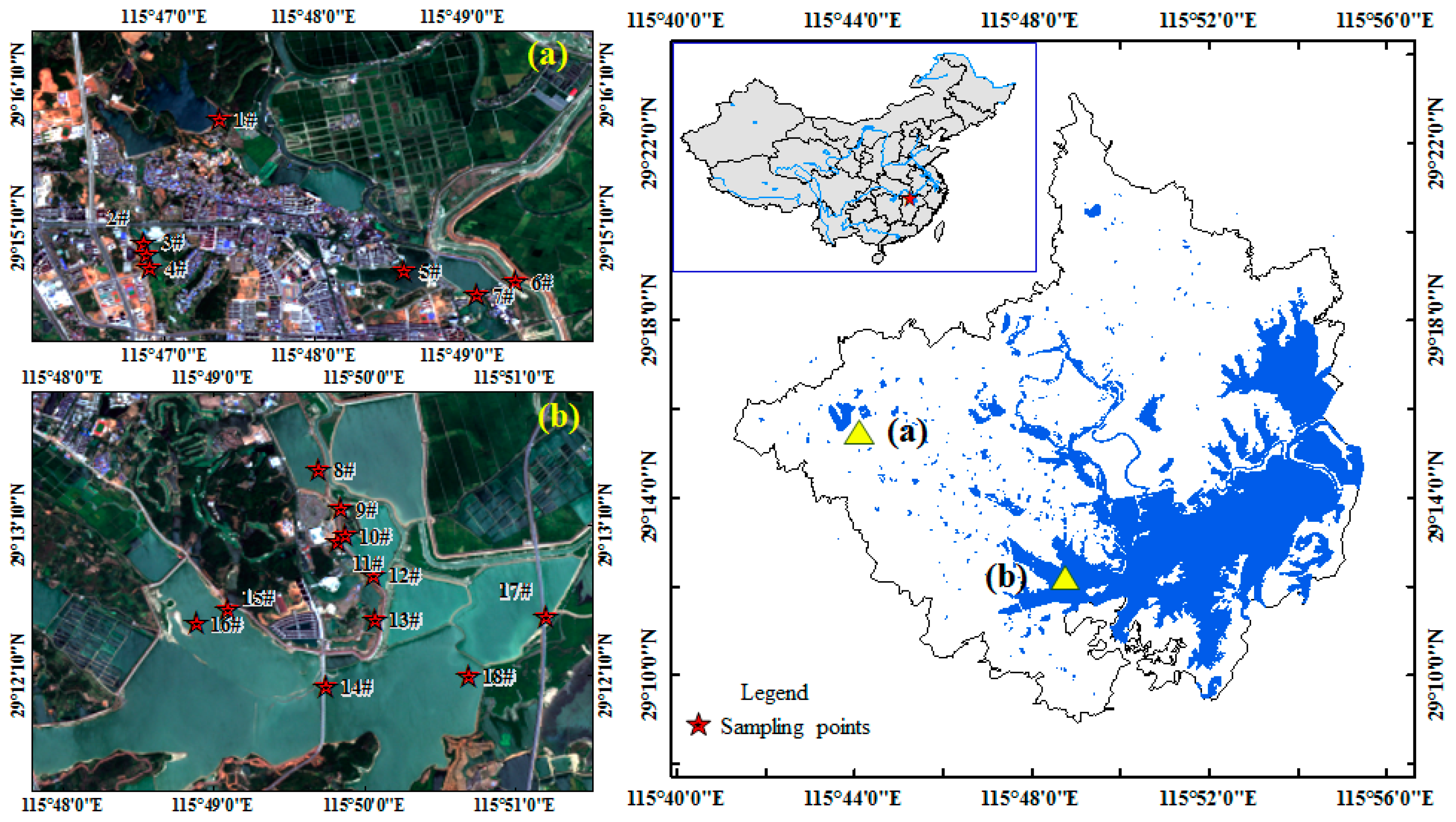
Gongqingcheng City is a hilly, lakeside city, located north of Jiangxi Province (29°09′–29°19′ N and 115°44′–115°58′ E) and adjacent to the northwestern shoreline of Poyang Lake, the largest freshwater lake in China. Gongqingcheng City’s main water bodies include the Boyang River, Nan Lake, and a branch of Poyang Lake. In addition, there are 19 dikes (with a total length of 71.3 km) and 21 reservoirs (with a total storage capacity of 9.6385 million m3). Gongqingcheng City has a subtropical, humid, monsoon climate with strongly seasonal hydrological characteristics. Average annual temperature and rainfall are 16.7 °C and 1395.6 mm, respectively [38]. Southerly winds prevail in the summer whilst northerly winds prevail through the rest of the year.
Before the large-scale urbanization began in 2010, the city’s water bodies were ecologically robust. In recent years, however, because of the expansion of industry, agriculture and fisheries, tons of urban sewage have been discharged into lakes and rivers. As a result, these water bodies have been experiencing increasingly severe eutrophication [39].
This research focuses on the period from 2018 to 2019, during which an environmental and ecological restoration program was launched in Gongqingcheng City. This program focused on the city’s water bodies and involved bank slope management, the dredging of rivers and lakes, and the restoration of water system connectivity.
2.2. Datasets and Preprocessing
2.2.1. Field Data
Monthly field measurements were conducted from November 2018 to October 2019. In order to representatively gauge the environmental characteristics and the trophic state of urban water bodies throughout the research area, a total of 18 sampling sites were identified in lakes, reservoirs, rivers and wetlands. The distribution of all sample sites is shown in Figure 1. Water samples from 50 cm below the surface were collected, and the concentrations of TP, CODMn, TN, and Chl-a were obtained by laboratory analysis within 48 h of the sample being taken. Simultaneously, SD and WT were measured during in situ surveys.
2.2.2. Satellite Data
‘Sentinel’ is a series of satellites launched by the European Commission (EC) and the European Space Agency (ESA) under the Copernicus program to meet specific Earth observation requirements. S-2 consists of two satellites (2A and 2B), with a phase difference of 180°, enabling a revisit period of only five days. The high spatial resolution of the S-2 satellites (13 spectral bands in the range of 400–2400 nm with 10, 20 and 60 m spatial resolution) makes them suitable for identifying and monitoring urban water bodies.
In order to estimate the TSI in an urban context, nine MSI images, covering Gongqingcheng City from November 2018 to October 2019, were downloaded from the ESA Data Hub, with time intervals of less than three days from sampling dates. The product level of MSI images is L1C, a top-of-atmosphere reflectance product with ortho-correction and geometric refinement at the sub-pixel level. Atmospherically corrected bottom-of-atmosphere reflectance, along with a scene classification map (L2A products), can be obtained from the L1C data using Sen2cor processing software provided by ESA.
2.2.3. Meteorological Data
Open source meteorological data corresponding to sampling dates were acquired from NOAA’s National Climatic Data Center. Variables of interest included air temperature (T), wind direction (WD) and wind speed (WS). The meteorological monitoring station closest to Gongqingcheng City is No.585060 (29°34′ N and 115°58′ E). Precipitation was not considered in our model because neither data collection nor RS image capture was possible on cloudy or rainy days.
3. Methods
3.1. Framework for TSI Estimation Model
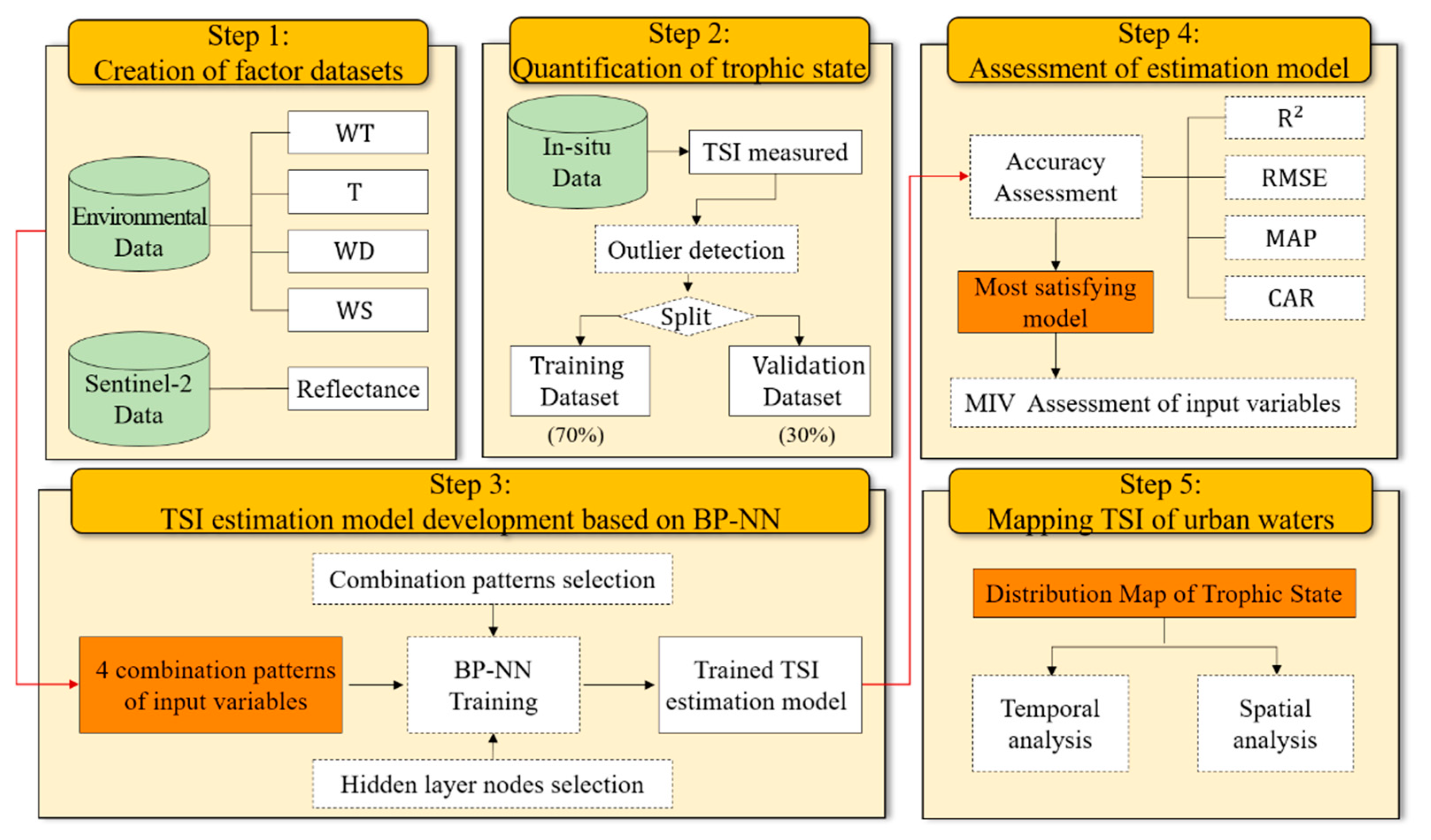
As shown in Figure 2, the framework of the TSI estimation model was based on a machine learning algorithm using S-2 data and environmental data as input variables. We set up four combination patterns of environmental and RS factors, selecting the most appropriate one by means of an accuracy assessment and a mean impact value (MIV) assessment. The final model, developed thus, was used to map the trophic state of urban waters.
3.2. Quantification of Trophic State
In this study, the trophic state of urban water bodies was quantified using a comprehensive evaluation method based on the trophic state index (TSI). This approach was proposed by the National Environmental Monitoring Center (NEMC) [40] and has been widely used in China for studying urban water trophic levels [41,42]. This method comprehensively considers the contribution degree of five trophic indicators, including Chl-a, TP, TN, SD and CODMn. The weight coefficients were obtained by extrapolating the correlation between Chl-a and other parameters, drawing on the statistical results of a survey of 26 major lakes in China. The expression for the TSI is:
where the unit of Chl-a is mg/m3, and the units of TP, TN, and CODMn are mg/L. SD represents the Secchi disk, where the unit is m. The larger the TSI, the higher the load of trophic indicators, thus the higher the incidence of eutrophication. The specific classifications were as follows: oligotrophic (TSI < 30), mesotrophic (30 ≤ TSI < 50), light eutrophic (50 ≤ TSI < 60), middle eutrophic (60 ≤ TSI < 70) and hypereutrophic (TSI ≥ 70).
3.3. Data Preprocessing
3.3.1. TSI Outlier Handling
Hydrogeological datasets often include substantial deviations, with a large number of points being designated ‘outliers’ as a result of errors in data measurement, transmission or transcription [43]. It is essential to ensure the reliability and accuracy of the original dataset prior to use. This can be achieved through data cleaning, especially in cases of data mining and machine learning where large sample sizes are standard [44].
Here, we introduce the inter-quartile range (IQR) rule for identifying TSI outliers because the IQR rule is not constrained by any dependence on, or assumption of, Gaussian data distributions. IQR is defined as the difference between the third and first quartiles, and elements >1.5 IQR larger than the third quartile (Q3), or <1.5 IQR smaller than the first quartile (Q1), are outliers, which are expressed as:
where and are the first and third quartiles of the sorted estimations, respectively.
3.3.2. Preprocessing of RS Images
Image preprocessing was performed using the SNAP and ENVI software packages [14]. This involved subsetting, resampling, reprojection, and the removal of cloud-pixel points. The region of interest (ROI) was defined as the administrative area of Gongqingcheng City. Geographically appropriate S-2 products were then resampled to 20 m resolution using a ‘bicubic’ interpolation method for up-sampling and a ‘median’ method for down-sampling. Some cloud-pixel points in the resampled images then needed to be removed by setting the threshold of the cloud confidence index to 20 so as to avoid cloud interference.
3.3.3. Extracting Water Bodies
In the case of S-2 satellite images, the Normalized Difference Water Index (NDWI)—calculated using Rrs from Band 3 (B3) and Band 8a (B8a)—is a more appropriate index for identifying open water bodies. The NDWI algorithm was developed by McFeeters [45] as a means of measuring water surface extent and can be defined as:
where and are the Rrs of B3 and B8a (from the S-2 data) respectively.
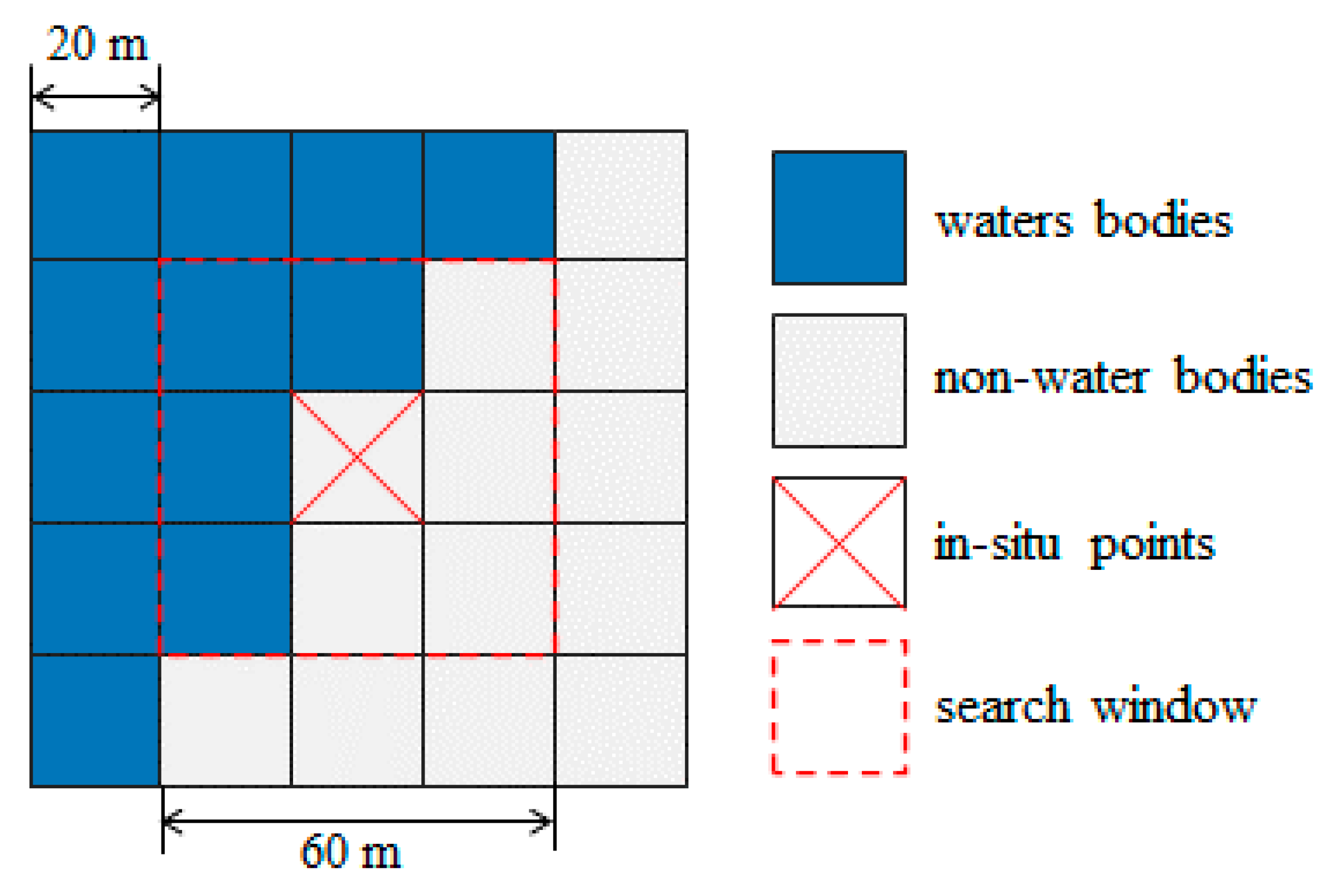
During the MSI data collection process, the measurable reflectance of water surfaces is affected by nearby structures, such as bridges and passing ships, and by factors such as water disturbance [46]. This is known as the adjacency effect, and was an important factor for consideration when analyzing water grids corresponding to in situ sampling points [28]. In this research, the nine-grid method was used to correct pixel points identified by the NDWI algorithm (Figure 3). This involved searching the pixel points located within a 3 × 3 window of each MSI image centered on the sampling point, extracting the water pixels amongst them and calculating the mean values of those water pixel points. If no water pixels were found to exist within the search window, the in situ point was deleted.
3.4. Estimation Modeling Techniques
3.4.1. Selection of Environmental Factors
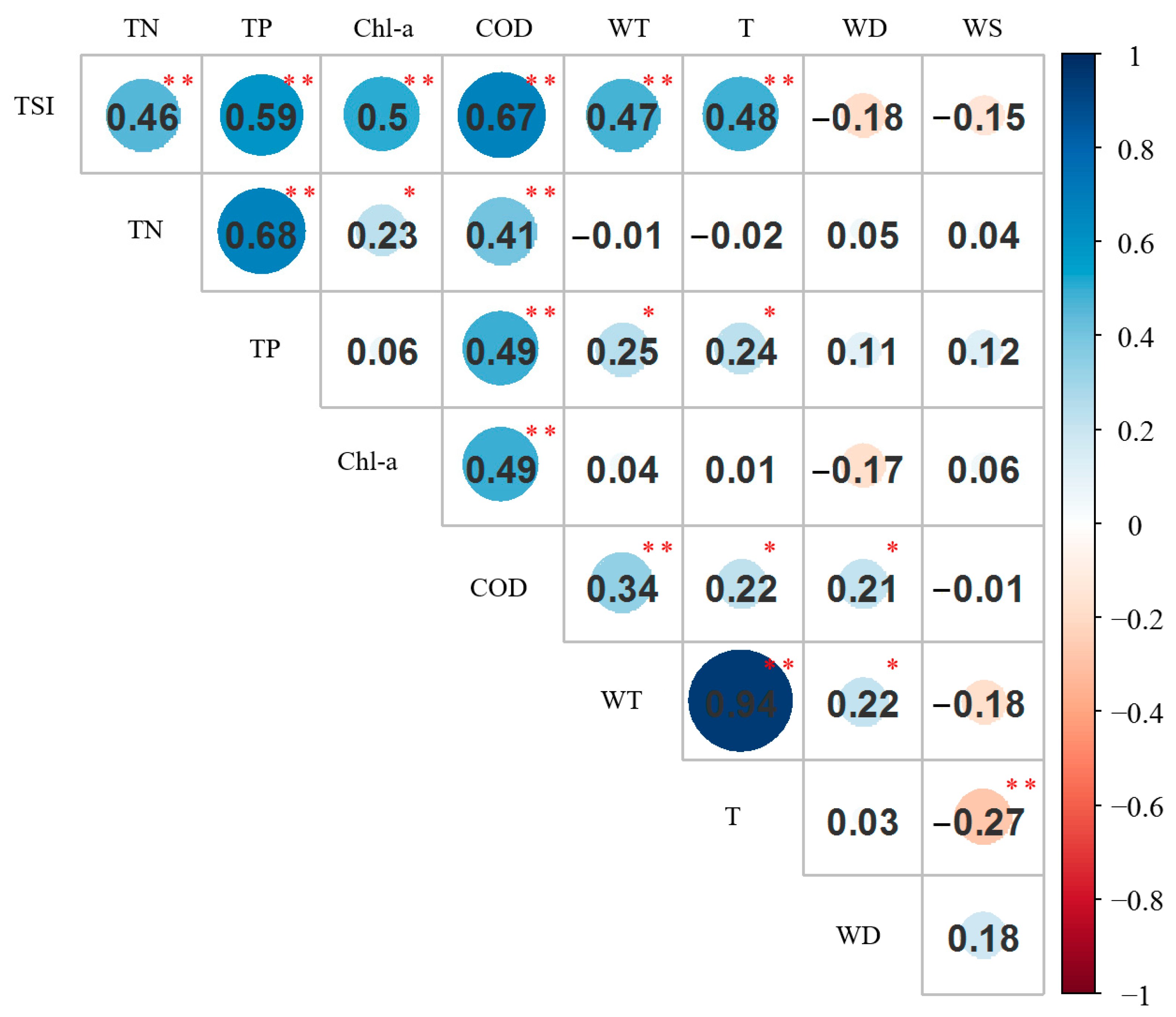
Four environmental factors were considered in this study: WT, T, WD and WS. First, the Pearson correlation coefficients between TSI, trophic indicators and these environmental factors were calculated to predict the influence these variables may have on the water body trophic state.
As is shown in Figure 4, both WT and T were strongly associated with TSI, showing similar correlation coefficients. These two environmental factors also displayed strong correlations with TP and CODMn, but no significant correlations with TN and Chl-a. As a result, WT and T were suitable for TSI estimation. Besides, there were no significant correlations between (1) WD and TSI and (2) WD and trophic indicators, except CODMn. However, the correlation coefficient between WD and Chl-a was highest amongst all the environmental factors, thus WD was alternatively selected as the input variable. There were no significant correlations between WS and TSI and all the trophic indicators, which may be attributable to the low levels of WS during the field survey. Therefore, WS was excluded from the estimation model.
Unfortunately, the correlation coefficients between independent variables were high, especially in the case of WT and T (correlation coefficient = 0.94), accounting for serious collinearity between the independent variables. Collinearity variables should not be input simultaneously to avoid estimation distortion of the prediction model.
3.4.2. TSI Estimation Model Based on Backpropagation Neural Network
Considering the complexity of trophic mechanisms within the aqueous environment, it is difficult to explain the relationships that exist between the TSI and the numerous influencing factors used in this study. It was in response to this fact that we introduced the BP-NN into the TSI recognition model. BP-NN is a multi-layer feedforward neural network, the main characteristics of which are signal forward propagation and error backpropagation [47].
The network structure of the BP-NN in this study is composed of three layers: the input layer, the hyperbolic tangent function hidden layer and the linear output layer. The environmental factors and RS factors were included in the input layer and the TSI in the output layer. The maximum number of training sessions was defined as 5000, while other parameters were set to default values. According to the universal approximation theorem [48], as long as the number of hidden layer nodes is appropriately defined within reasonable limits, a three-layer NN can be effectively applied to a wide range of problems [49]. This being the case, the number of hidden layer nodes in this study was optimized by means of a test analysis, run in order to obtain the optimal fitting results. We then set up four combination patterns of input variables (Table 1) representative of different water conditions, and defined the optimal combinations based on the accuracy assessment of the BP-NN output.
3.4.3. TSI Estimation Model Based on Backpropagation Neural Network
MIV was used to determine the influence of input neurons on the output neurons within the BP-NN model. The specific process followed in performing this calculation was as follows [50]: After network training had been concluded, the training samples of each input variable were used to form two new training samples based on its original value, plus or minus 10%. The application of the developed network was built in the new training sample, and two simulation results were obtained. The difference of the simulation results represented the influence on TSI induced by each input variable.
3.4.4. Assessment of the Accuracy of the Model
The accuracy of the developed model could be measured through the coefficient of determination (), root mean square error (RMSE), mean absolute percentage error (MAPE) and classification accuracy rate (CAR). These four parameters were calculated as follows:
where y is the value of TSI measured using in situ data, f is the estimated TSI value, n is the number of all samples, is the classification based on TSI and is the indicator function.
4. Results
4.1. TSI Level and S-2 Spectral Characteristics
Because the study area was obscured by thick clouds throughout January, February and April 2019, all S-2 imagery acquired during these three months was omitted from this study. Subsequent to data preprocessing, TSI results of 110 samples were obtained for the region for the period from 2018 to 2019 (Figure 5). Due to the high trophic load of shallow urban lakes, water fluidity was lacking and the eutrophication was severe, with the average TSI fluctuating between 58 and 80. Additionally, the TSI of the studied urban water bodies exhibited pronounced seasonal heterogeneity. Temperatures rose in spring and remained high throughout summer, providing favorable conditions for phytoplankton growth. During this annual warm period, it was observed that the TSI increases monthly, peaking at over 80 (severe eutrophication) in August. In addition to seasonal differences, TSI also showed up spatial heterogeneity in reservoirs, rivers and lakes. Specifically, a reservoir represented by the 1# sampling point was in the mesotrophic state, with a TSI of around 44 during the study period. The river typed urban waters, represented by the 7# survey point, were mainly in the light eutrophic state, with an average TSI of around 59. For most of the urban lakes, the eutrophication problems appeared in different degrees.
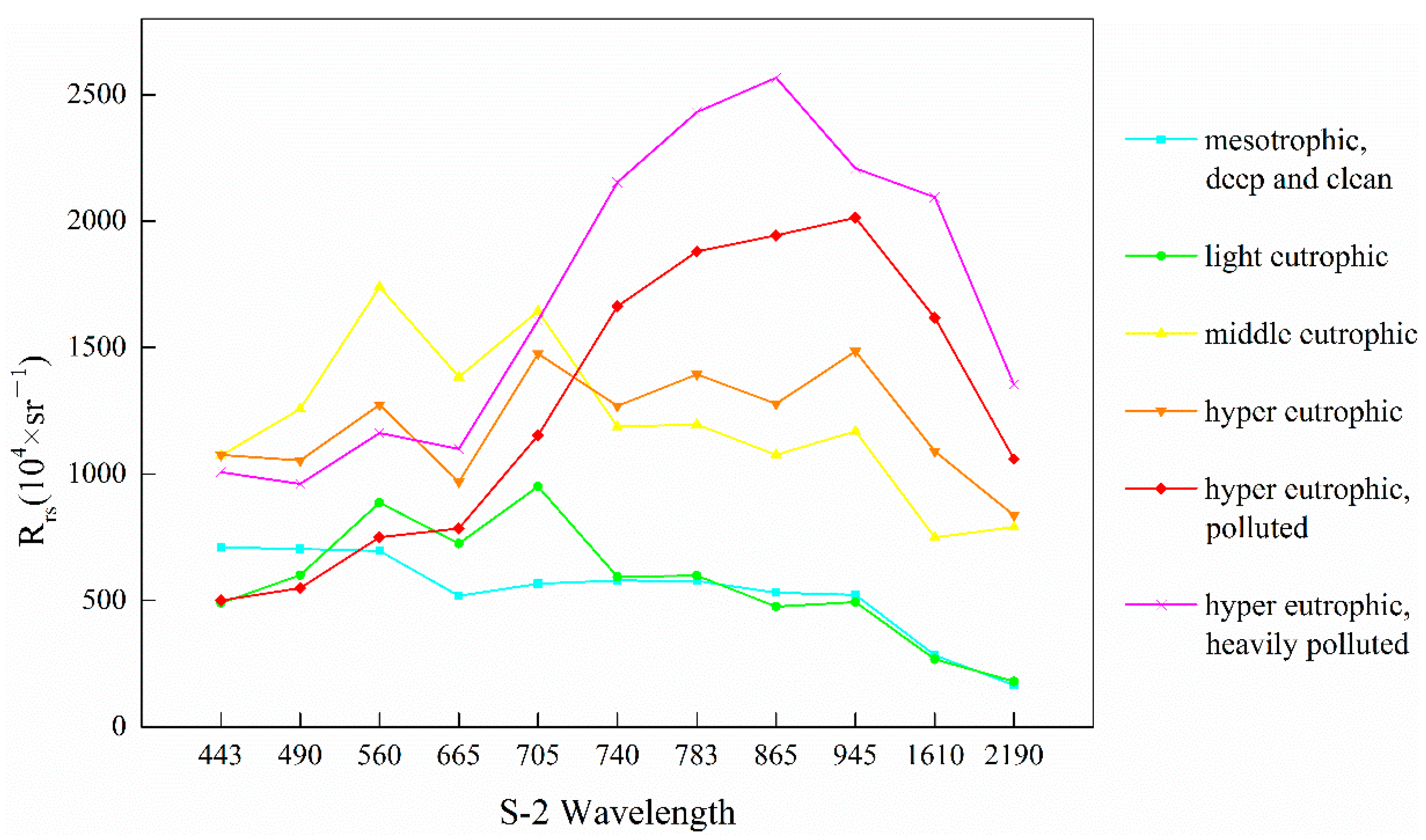
In order to explore the differences of spectral characteristics within different water trophic states, the typical spectra for S-2 MSI bands were selected for each of the four TSI grades, ranging from mesotrophic to hypereutrophic (Figure 6). The mesotrophic curve was obtained using measurements taken from the reservoir within the study area, where water quality was still high. The middle eutrophic curve and the first hypereutrophic curve corresponded to the same urban water body in the months of July and September, respectively. The last two hypereutrophic curves describe the effluents of a sewage treatment plant in the months of August and October (respectively). A significant peak was observed in B3 and B5 and a slight reflectance trough can be seen in B4, representing eutrophic water, where B3 is the minimum absorption band of chlorophyll, B4 can reflect the chlorophyll fluorescence effect, and B5 is the special vegetation red edge band of the S-2 products. Those bands are also sensitive for algal blooms [35]. The reflectance of the deep reservoir shown by the blue curve is relatively low, resulting in an indistinct spectral feature.
4.2. TSI Estimation Using Environmental Factors
4.2.1. Comparison of the Performances of the TSI Estimation Model with Environmental Factors
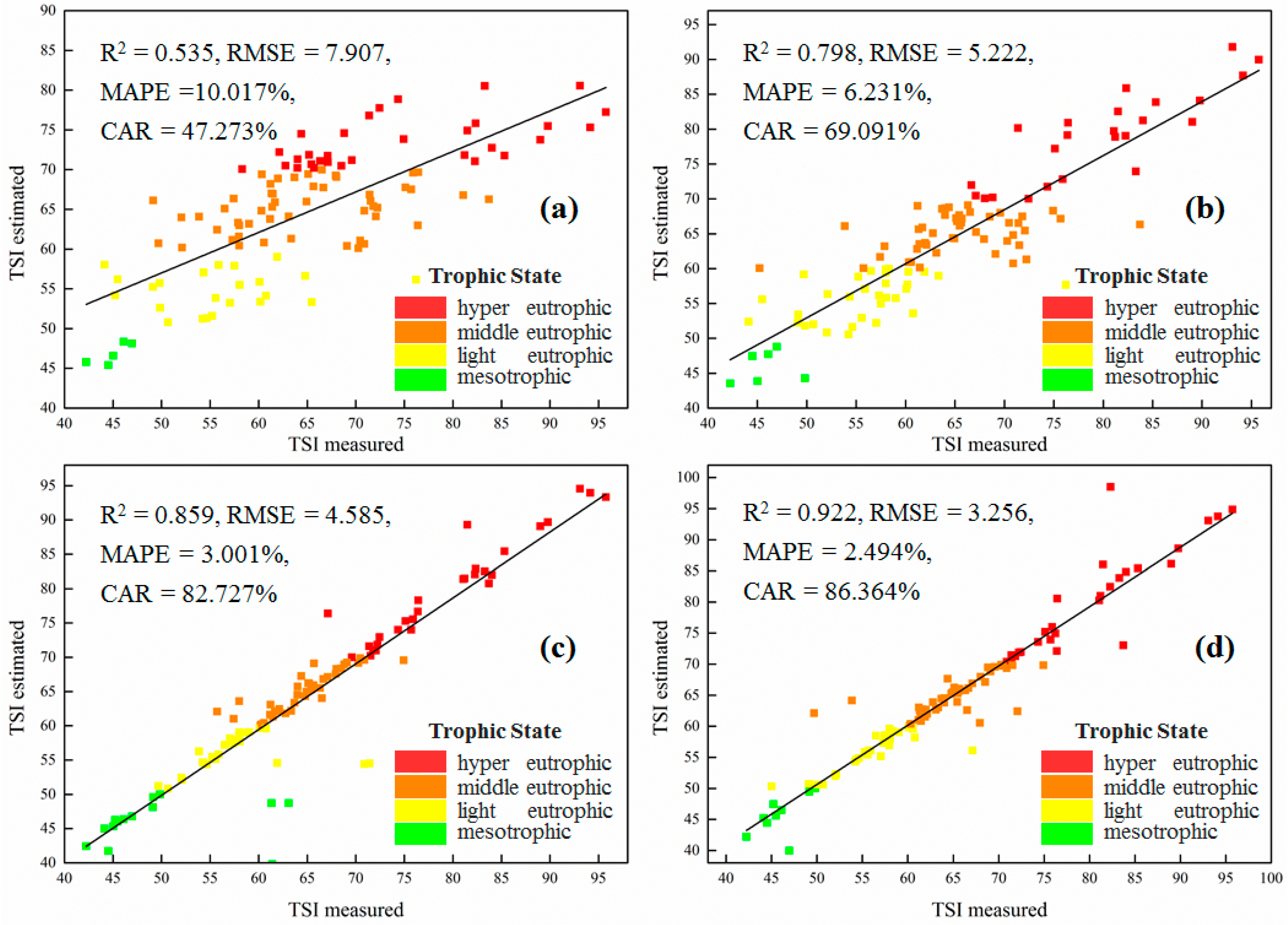
During this study, it was observed that the error tended to stabilize when the number of hidden layer nodes for each test was set to 12 (Table A1). Distributions of both the TSI estimated from the BP-NN model and the measured TSI values are shown in Figure 7. Initially, the model ran with only RS factors (Figure 7a), but its accuracy improved significantly following the addition of environmental factors. The CAR of the model combined with the T factor (Figure 7b) improved by 22% when compared with the original model. Among the three combinations of environmental factors utilized, the TSI estimation model combined with WT (Figure 7d) had the highest accuracy and determination coefficient (R2 = 0.977, RMSE = 3.256, MAPE = 2.494%). This combination also achieved the highest accuracy for trophic classification (CAR = 86.364%). However, the accuracy of the model combined with WT and WD (Figure 7c) decreased, underestimating a few scattered points in the light and middle eutrophic states and showing a deviation from the tropic line. This may have been the result of environmental variable redundancy, reducing the predictive capability of the model. From the above results we can deduce that WT is more suitable as an input variable for the estimation of TSI than T or WD. The significance of WT with regards to the water trophic state is discussed in Section 5.
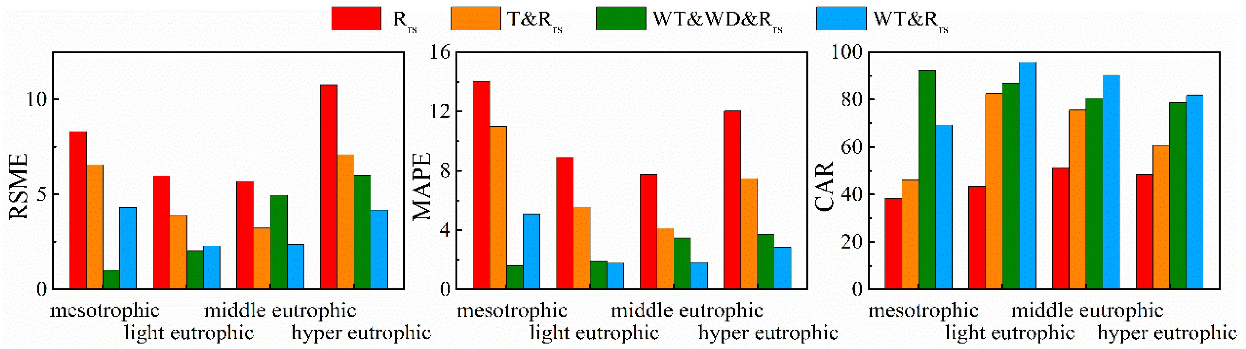
We further analyzed the WT-Rrs combined model’s ability to generalize the different trophic levels of water bodies. As shown in Figure 8, the model produced a high estimation accuracy when it identified areas of light and middle eutrophication (50 < TSI < 70), even when the model was run without environmental factor inputs. When mesotrophic and hypereutrophic water bodies were concerned (TSI < 50 or TSI > 70), the estimation model produced more significant estimation and classification errors. The WT-Rrs combined estimation model demonstrated a higher classification accuracy in the case of hypereutrophic waters (CAR = 81.82%), making it suitable for use in places where urban water bodies exhibit eutrophication problems.
4.2.2. Mean Impact Value Analysis
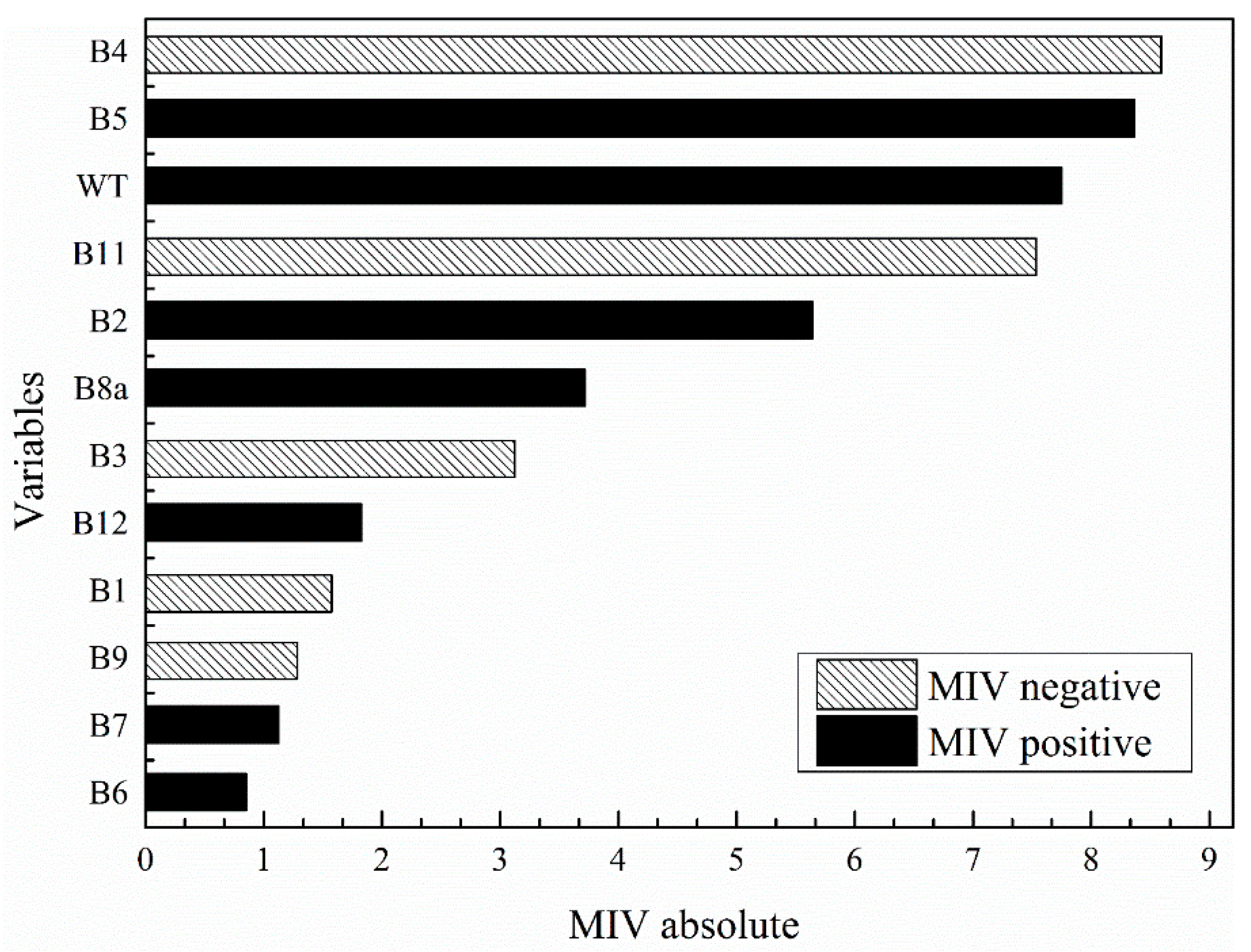
The importance of each input variable involved in the WT-Rrs combined estimation model was evaluated, and the absolute MIV distribution of variables is shown in Figure 9.
The reflectance values in B4 and B5 ranked most highly among all the variables, although they show opposite effects on TSI estimation (B4 is negative whilst B5 is positive). The prominence of these bands represents the chlorophyll fluorescence effect and the vegetation red edge effect. WT also had a high MIV on the estimated results, reflecting the importance of environmental factors in determining the trophic state. In addition, the MIV of B11 and B2 (−7.5350 and 5.6419, respectively) trailed closely behind that of WT. MIV scores in the red-edge bands (B6 and B7) were lowest, at approximately 1.0.
4.3. Temporal and Spatial Distribution of Trophic State
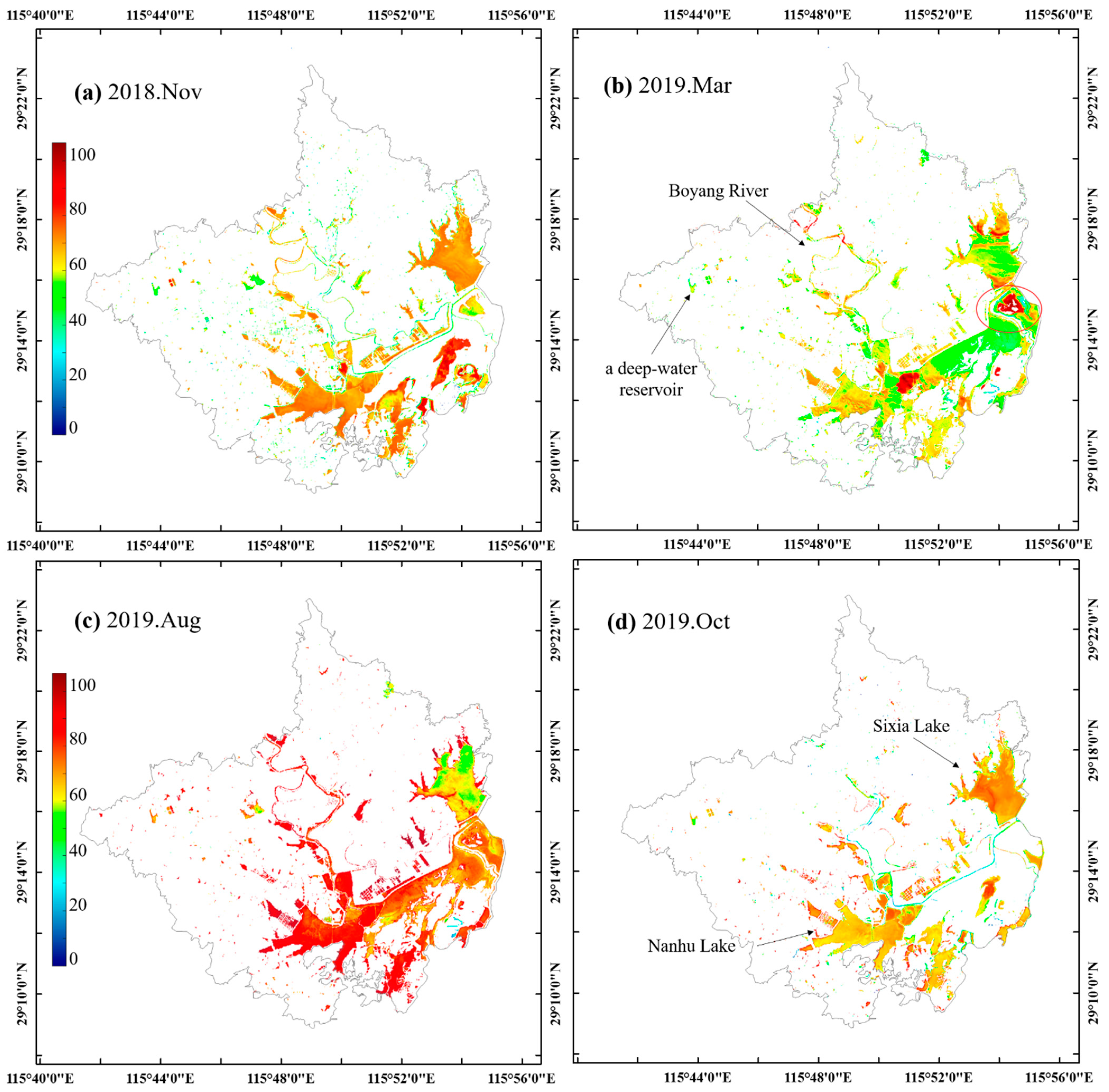
The BP-NN model, integrating the WT and Rrs of S-2 was used to map the spatial distribution of TSI with respect to water bodies throughout the study area over a period of four months between 2018 and 2019. Figure 10 shows changes in the water area and trophic state in the study area over time. The predicted distribution of TSI in the four stages fits well with our previous, existing understanding of this region.
The TSI values modelled for urban water bodies in Gongqingcheng City displayed a seasonal pattern of lower values in winter and higher values in summer. This conforms to apparent seasonal variations in nutrient levels; examples of the latter include TP, TN, and Chl-a. Additionally, lower trophic levels were observed in rivers and reservoirs than in lakes.
The area of water classified as being eutrophic decreased between the winter of 2018 and October 2019, especially in the part of Nanhu Lake that adjoins to Poyang Lake. This observation shows that the restoration project helped to alleviate eutrophication in the study area.
The water bodies examined in this study underwent the most pronounced eutrophication during the summer months (Figure 10c). With the exception of Sixia Lake (in the north of the study area), nearly 80% of the water bodies in this region exhibited a TSI > 70. Of those water bodies, the Boyang River (which flows into the South Lake) appeared to undergo the most significant changes.
Unfortunately, the predicted TSI value corresponding to the triangular water area, shown in dark red in Figure 10b, is too high. This is perhaps because the area in question is a wetland during the dry season, and the water is relatively shallow at that time (no water was detected in Figure 10d). The optical characteristics of this locale are therefore different to those of a more ‘conventional’ water body. This affects the modelling result. Clearly, further work is required in this area.
5. Discussion
WT exhibits a rapid and direct response to climatic forcing [51,52,53]. Previous studies have indicated that WT is the main driving factor behind water eutrophication. Studies have also shown that it plays a vital role in the recovery and growth of cyanobacteria, making WT a key variable in the formation, decline and large-scale outbreak of algal bloom events [1]. RS images can be used to effectively gauge the trophic state, enabling us to identify areas undergoing increased eutrophication. This is made possible because the increase in productivity associated with eutrophication is accompanied by a change in the optical properties of water [20].
In this study, we coupled ‘influence variables’ with ‘state variables’; that is to say, the variable of WT was fed into the TSI estimation model so as to supply information that is difficult to extract from remotely sensed images. The MIV method was then used to assess the relative importance of different variables in terms of their effect on trophic state. The BP-NN is a non-linear black-box model that can simplify both the variables fed into the model and the process of model fitting to ensure the robustness of the algorithm and reduce the risk of overfitting.
Our results show that WT is not only strongly correlated with TSI, but also exerts a significant influence on the estimation of TSI. Therefore, in cases where urban water trophic state is being modelled, using long time series data and on a large geographic scale, we suggest that WT be taken as an input variable to improve the accuracy and temporal and spatial portability of the model. This ease of use should enable water management authorities anywhere in the world to employ the method, contributing to the scientific management of urban water environments on a global scale.
It should be noted that the NN model needs to be supported by large-scale sampling data [26,54]. Due to the lack of available monitoring data for non-eutrophic water bodies, the accuracy of this model cannot be verified for water bodies with a TSI < 30. Furthermore, the model occasionally underestimates sample points with a TSI < 50, which is the same as the result from Watanabe et al. [27]. It is likely that the similarity between mesotrophic and light eutrophic samples measured by S-2 Rrs (Figure 6), and the limitations in S-2 spectral bands, interfere with the identification of the trophic state, thereby contributing to this issue [55]. We encourage other researchers to apply this model to urban water bodies elsewhere so as to further validate and improve our method.
6. Conclusions
A BP-NN-based TSI estimation model is proposed for the analysis of urban water bodies. The established model is superior to alternative methods in several ways: (i) unlike the traditional RS models, both environmental factors (influencing variables) and satellite images (current ‘state’ variables) are considered, and WT is demonstrated to be the most important variable for TSI estimation; (ii) the machine learning approach based on the BP-NN algorithm is trained and substantiated using in situ datasets (n = 110) covering the typical period of one year in urban waters. The high accuracy of the WT-Rrs combined estimation model suggests that environmental factors can compensate for the insufficiency of remotely sensed estimation methods to accurately monitor trophic state. Our integrated methodology enables spatial and temporal distribution maps of TSI to be produced and effectively evaluates the trophic state of urban water bodies.
Author Contributions
Conceptualization, S.Z., and J.M.; methodology, S.Z.; software, S.Z.; validation, S.Z.; formal analysis, S.Z.; investigation, S.Z.; resources, J.M.; data curation, S.Z., and J.M.; writing—original draft preparation, S.Z.; writing—review and editing, J.M.; visualization, S.Z.; supervision, J.M.; project administration, J.M.; funding acquisition, J.M. All authors have read and agreed to the published version of the manuscript.
Funding
This research was funded by the National Key Research and Development Program of China (Grant No. 2018YFC0407606).
Institutional Review Board Statement
Not applicable.
Informed Consent Statement
Not applicable.
Data Availability Statement
The data presented in this study are available on request from the corresponding author.
Acknowledgments
The authors wish to acknowledge all study participants from Nanjing Institute of Geography and Limnology, Chinese Academy of Sciences and Jiangxi Academy of Water Science and Engineering for field work support.
Conflicts of Interest
The authors declare no conflict of interest.
Appendix A

Table A1.
Effect of the hidden layer size on WT-Rrs combined model. The No.8 test in bold shows the optimal hidden layer size.
Table A1.
Effect of the hidden layer size on WT-Rrs combined model. The No.8 test in bold shows the optimal hidden layer size.
| No. | Hidden Layer Size | R2 | RMSE | MAPE |
|---|---|---|---|---|
| 1 | 5 | 0.8353 | 4.7017 | 4.9326 |
| 2 | 6 | 0.8260 | 4.8652 | 5.8568 |
| 3 | 7 | 0.7332 | 6.0059 | 7.6803 |
| 4 | 8 | 0.8490 | 4.5014 | 4.5445 |
| 5 | 9 | 0.8401 | 4.6384 | 4.7116 |
| 6 | 10 | 0.8417 | 4.6497 | 3.8771 |
| 7 | 11 | 0.9104 | 3.4849 | 3.7089 |
| 8 | 12 | 0.9220 | 3.2559 | 2.4944 |
| 9 | 13 | 0.8211 | 5.0092 | 2.5062 |
| 10 | 14 | 0.8030 | 5.2856 | 3.5363 |
References
- Chen, Q.; Huang, M.; Tang, X. Eutrophication assessment of seasonal urban lakes in China Yangtze River Basin using Landsat 8-derived Forel-Ule index: A six-year (2013–2018) observation. Sci. Total Environ. 2020, 745, 135392. [Google Scholar] [CrossRef] [PubMed]
- Yang, Y.; Bai, Y.; Wang, X.; Wang, L.; Jin, X.; Sun, Q. Group Decision-Making Support for Sustainable Governance of Algal Bloom in Urban Lakes. Sustainability 2020, 12, 1494. [Google Scholar] [CrossRef] [Green Version]
- Hutchinson, G.E. Eutrophication: Causes, Consequences, Correctives; The National Academies Press: Washington, DC, USA, 1969; p. 670. [Google Scholar]
- Matthews, M.; Bernard, S. Eutrophication and cyanobacteria in South Africa’s standing water bodies: A view from space. S. Afr. J. Sci. 2015, 111, 1–8. [Google Scholar] [CrossRef] [Green Version]
- Carlson, R. A Trophic State Index for Lakes. Limnol. Oceanogr. 1977, 22, 361–369. [Google Scholar] [CrossRef] [Green Version]
- Dörnhöfer, K.; Oppelt, N. Remote sensing for lake research and monitoring–Recent advances. Ecol. Indic. 2016, 64, 105–122. [Google Scholar] [CrossRef]
- Tyler, A.N.; Hunter, P.D.; Spyrakos, E.; Groom, S.; Constantinescu, A.M.; Kitchen, J. Developments in Earth observation for the assessment and monitoring of inland, transitional, coastal and shelf-sea waters. Sci. Total Environ. 2016, 572, 1307–1321. [Google Scholar] [CrossRef] [PubMed] [Green Version]
- Dekker, A.G.; Peters, S.W.M. The use of the Thematic Mapper for the analysis of eutrophic lakes: A case study in The Netherlands. Int. J. Remote Sens. 1993, 14, 799–821. [Google Scholar] [CrossRef]
- Olmanson, L.G.; Bauer, M.E.; Brezonik, P.L. A 20-year Landsat water clarity census of Minnesota’s 10,000 lakes. Remote Sens. Environ. 2008, 112, 4086–4097. [Google Scholar] [CrossRef]
- Park, Y.-J.; Ruddick, K.; Lacroix, G. Detection of algal blooms in European waters based on satellite chlorophyll data from MERIS and MODIS. Int. J. Remote Sens. 2010, 31, 6567–6583. [Google Scholar] [CrossRef]
- Torbick, N.; Hession, S.; Hagen, S.; Wiangwang, N.; Becker, B.; Qi, J. Mapping inland lake water quality across the Lower Peninsula of Michigan using Landsat TM imagery. Int. J. Remote Sens. 2013, 34, 7607–7624. [Google Scholar] [CrossRef]
- Ross, M.R.V.; Topp, S.N.; Appling, A.P.; Yang, X.; Kuhn, C.; Butman, D.; Simard, M.; Pavelsky, T.M. AquaSat: A Data Set to Enable Remote Sensing of Water Quality for Inland Waters. Water Resour. Res. 2019, 55, 10012–10025. [Google Scholar] [CrossRef]
- Shi, K.; Zhang, Y.; Song, K.; Liu, M.; Zhou, Y.; Zhang, Y.; Li, Y.; Zhu, G.; Qin, B. A semi-analytical approach for remote sensing of trophic state in inland waters: Bio-optical mechanism and application. Remote Sens. Environ. 2019, 232, 111349. [Google Scholar] [CrossRef]
- Watanabe, F.S.Y.; Alcântara, E.; Rodrigues, T.W.P.; Imai, N.N.; Barbosa, C.C.F.; Rotta, L.H.d.S. Estimation of Chlorophyll-a Concentration and the Trophic State of the Barra Bonita Hydroelectric Reservoir Using OLI/Landsat-8 Images. Int. J. Environ. Res. Pub. He. 2015, 12, 10391–10417. [Google Scholar] [CrossRef]
- Duan, H.; Zhang, Y.; Zhang, B.; Song, K.; Wang, Z.; Liu, D.; Li, F. Estimation of chlorophyll—A concentration and trophic states for inland lakes in Northeast China from Landsat TM data and field spectral measurements. Int. J. Remote Sens. 2008, 29, 767–786. [Google Scholar] [CrossRef]
- Novo, E.M.L.d.M.; Londe, L.d.R.; Barbosa, C.; Araujo, C.A.S.d.; Rennó, C.D. Proposal for a remote sensing trophic state index based upon Thematic Mapper/Landsat images. Rev. Ambiente Água 2013, 8, 65–82. [Google Scholar]
- Thiemann, S.; Kaufmann, H. Determination of Chlorophyll Content and Trophic State of Lakes Using Field Spectrometer and IRS-1C Satellite Data in the Mecklenburg Lake District, Germany. Remote Sens. Environ. 2000, 73, 227–235. [Google Scholar] [CrossRef]
- Sheela, A.M.; Letha, J.; Joseph, S.; Ramachandran, K.K.; Sanalkumar, S.P. Trophic state index of a lake system using IRS (P6-LISS III) satellite imagery. Environm. Monit. Assess. 2011, 177, 575–592. [Google Scholar] [CrossRef]
- Lillesand, T.M.; Johnson, W.l.; Deuell, R.L.; Lindstrom, O.M.; Meisener, D.E. Use of Landsat data to predict the trophic state of Minnesota lakes. Photogramm. Eng. REM S 1983, 49, 219–229. [Google Scholar]
- Baban, S.M.J. Trophic classification and ecosystem checking of lakes using remotely sensed information. Hydrolog. Sci. J. 1996, 41, 939–957. [Google Scholar] [CrossRef] [Green Version]
- Isenstein, E.M.; Park, M.H. Assessment of nutrient distributions in Lake Champlain using satellite remote sensing. J. Environ. Sci. 2014, 26, 1831–1836. [Google Scholar] [CrossRef] [PubMed]
- Song, K.; Li, L.; Li, S.; Tedesco, L.; Hall, B.; Li, L. Hyperspectral Remote Sensing of Total Phosphorus (TP) in Three Central Indiana Water Supply Reservoirs. Water Air Soil Pollut. 2011, 223, 1481–1502. [Google Scholar] [CrossRef]
- Cao, Y.; Ye, Y.; Liang, L.; Zhao, H.; Jiang, Y.; Wang, H.; Yan, D. Remote sensing retrieval of chlorophyll-α in inland waters based on ensemble modeling: A case study on Panjiakou and Daheiting reservoirs. J. Appl. Remote Sens. 2020, 14, 024503. [Google Scholar] [CrossRef]
- Cheng, K.-S.; Lei, T.-C. Reservoir trophic state evaluation using lanisat TM images. J. Am. Water Resour. As. 2001, 37, 1321–1334. [Google Scholar] [CrossRef]
- González Vilas, L.; Spyrakos, E.; Torres Palenzuela, J.M. Neural network estimation of chlorophyll a from MERIS full resolution data for the coastal waters of Galician rias (NW Spain). Remote Sens. Environ. 2011, 115, 524–535. [Google Scholar] [CrossRef]
- Pahlevan, N.; Smith, B.; Schalles, J.; Binding, C.; Cao, Z.; Ma, R.; Alikas, K.; Kangro, K.; Gurlin, D.; Hà, N.; et al. Seamless retrievals of chlorophyll-a from Sentinel-2 (MSI) and Sentinel-3 (OLCI) in inland and coastal waters: A machine-learning approach. Remote Sens. Environ. 2020, 240, 111604. [Google Scholar] [CrossRef]
- Watanabe, F.S.Y.; Miyoshi, G.T.; Rodrigues, T.W.P.; Bernardo, N.M.R.; Rotta, L.H.S.; Alcântara, E.; Imai, N.N. Inland water’s trophic status classification based on machine learning and remote sensing data. Remote Sens. Appl. Soc. Environ. 2020, 19, 100326. [Google Scholar] [CrossRef]
- Palmer, S.C.J.; Kutser, T.; Hunter, P.D. Remote sensing of inland waters: Challenges, progress and future directions. Remote Sens. Environ. 2015, 157, 1–8. [Google Scholar] [CrossRef] [Green Version]
- Peng, J.J.; Li, C.H. Causes and characteristics of eutrophication in urban lakes. Ecol. Sci. 2004, 23, 370–373. [Google Scholar]
- Dierssen, H.; Zimmerman, R.; Leathers, R.; Downes, T.; Davis, C. Remote sensing of seagrass and bathymetry in the Bahamas Banks using high resolution aerial imagery. Limnol. Oceanogr. 2003, 48, 444–455. [Google Scholar] [CrossRef]
- Hu, M.; Ma, R.; Cao, Z.; Xiong, J.; Xue, K. Remote Estimation of Trophic State Index for Inland Waters Using Landsat-8 OLI Imagery. Remote Sens. 2021, 13, 1988. [Google Scholar] [CrossRef]
- Lu, X.; Lu, Y.; Chen, D.; Su, C.; Song, S.; Wang, T.; Tian, H.; Liang, R.; Zhang, M.; Khan, K. Climate change induced eutrophication of cold-water lake in an ecologically fragile nature reserve. J. Environ. Sci. 2019, 75, 359–369. [Google Scholar] [CrossRef]
- Mao, J.Q.; Lee, J.H.W.; Choi, K.W. The extended Kalman filter for forecast of algal bloom dynamics. Water Res. 2009, 43, 4214–4224. [Google Scholar] [CrossRef]
- Jørgensen, S.E.; Mitsch, W.J. Application of Ecological Modelling in Environmental Management. Elsevier Scientific Publishing Company: Amsterdam, The Netherlands; Oxford, UK; New York, NY, USA, 1983. [Google Scholar]
- Ma, J.; Jin, S.; Li, J.; He, Y.; Shang, W. Spatio-Temporal Variations and Driving Forces of Harmful Algal Blooms in Chaohu Lake: A Multi-Source Remote Sensing Approach. Remote Sens. 2021, 13, 427–440. [Google Scholar] [CrossRef]
- Wang, Z.; Liu, J.; Li, J.; Meng, Y.; Pokhrel, Y.; Zhang, H. Basin-scale high-resolution extraction of drainage networks using 10-m Sentinel-2 imagery. Remote Sens. Environ. 2021, 255, 112281. [Google Scholar] [CrossRef]
- Brisset, M.; Van Wynsberge, S.; Andréfouët, S.; Payri, C.; Soulard, B.; Bourassin, E.; Gendre, R.L.; Coutures, E. Hindcast and Near Real-Time Monitoring of Green Macroalgae Blooms in Shallow Coral Reef Lagoons Using Sentinel-2: A New-Caledonia Case Study. Remote Sens. 2021, 13, 211. [Google Scholar] [CrossRef]
- Zhu, H.; Xu, L.; Jiang, J.; Fan, H. Spatiotemporal Variations of Summer Precipitation and Their Correlations with the East Asian Summer Monsoon in the Poyang Lake Basin, China. Water 2019, 11, 1705. [Google Scholar] [CrossRef] [Green Version]
- Huang, W.; Mao, J.; Zhu, D.; Lin, C. Impacts of Land Use and Land Cover on Water Quality at Multiple Buffer-Zone Scales in a Lakeside City. Water 2020, 12, 47. [Google Scholar] [CrossRef] [Green Version]
- Wang, M.; Liu, X.; Zhang, J. Evaluate method and classification standard on lake eutrophication. Environmental Monitoring in China 2002, 18, 47–49. [Google Scholar]
- Wang, J.; Fu, Z.; Qiao, H.; Liu, F. Assessment of eutrophication and water quality in the estuarine area of Lake Wuli, Lake Taihu, China. Sci. Total Environ. 2019, 650, 1392–1402. [Google Scholar] [CrossRef]
- Zhi, G.; Chen, Y.; Liao, Z.; Walther, M.; Yuan, X. Comprehensive assessment of eutrophication status based on Monte Carlo–triangular fuzzy numbers model: Site study of Dongting Lake, Mid-South China. Environ. Earth Sci. 2016, 75, 1011. [Google Scholar] [CrossRef]
- Jeong, J.; Park, E.; Han, W.S.; Kim, K.; Choung, S.; Chung, I.M. Identifying outliers of non-Gaussian groundwater state data based on ensemble estimation for long-term trends. J. Hydrol. 2017, 548, 135–144. [Google Scholar] [CrossRef]
- Maletic, J.I.; Marcus, A. Data Cleansing: Beyond Integrity Analysis. In Proceedings of the Fifth Conference on Information Quality, Cambridge, MA, USA, January 2000; pp. 200–209. [Google Scholar]
- McFeeters, S.K. The use of the Normalized Difference Water Index (NDWI) in the delineation of open water features. Int. J. Remote Sens. 1996, 17, 1425–1432. [Google Scholar] [CrossRef]
- Tavares, M.H.; Cunha, A.H.F.; Motta-Marques, D.; Ruhoff, A.L.; Fragoso, C.R.; Munar, A.M.; Bonnet, M.-P. Derivation of consistent, continuous daily river temperature data series by combining remote sensing and water temperature models. Remote Sens. Environ. 2020, 241, 111721. [Google Scholar] [CrossRef]
- Rumelhart, D.E.; Hinton, G.E.; Williams, R.J. Learning representations by back-propagating errors. Nature 1986, 323, 533–536. [Google Scholar] [CrossRef]
- Cybenko, G.V. Approximation by superpositions of a sigmoidal function. Math. Control Signals Syst. 1992, 5, 455. [Google Scholar] [CrossRef] [Green Version]
- Dayhoff, J.E.; DeLeo, J.M. Artificial neural networks. Cancer 2001, 91, 1615–1635. [Google Scholar] [CrossRef]
- Dombi, G.W.; Nandi, P.; Saxe, J.M.; Ledgerwood, A.M.; Lucas, C.E. Prediction of rib fracture injury outcome by an artificial neural network. J. Trauma 1995, 39, 915–921. [Google Scholar] [CrossRef] [PubMed]
- Adrian, R.; O’Reilly, C.M.; Zagarese, H.; Baines, S.B.; Hessen, D.O.; Keller, W.; Livingstone, D.M.; Sommaruga, R.; Straile, D.; Van Donk, E.; et al. Lakes as sentinels of climate change. Limnol. Oceanogr. 2009, 54, 2283–2297. [Google Scholar] [CrossRef] [PubMed]
- O’Neil, J.M.; Davis, T.W.; Burford, M.A.; Gobler, C.J. The rise of harmful cyanobacteria blooms: The potential roles of eutrophication and climate change. Harmful Algae 2012, 14, 313–334. [Google Scholar] [CrossRef]
- Paerl, H.W.; Huisman, J. Climate change: A catalyst for global expansion of harmful cyanobacterial blooms. Environ. Microbiol. Rep. 2009, 1, 27–37. [Google Scholar] [CrossRef]
- Nickmilder, C.; Tedde, A.; Dufrasne, I.; Lessire, F.; Tychon, B.; Curnel, Y.; Bindelle, J.; Soyeurt, H. Development of Machine Learning Models to Predict Compressed Sward Height in Walloon Pastures Based on Sentinel-1, Sentinel-2 and Meteorological Data Using Multiple Data Transformations. Remote Sens. 2021, 13, 408. [Google Scholar] [CrossRef]
- Sent, G.; Biguino, B.; Favareto, L.; Cruz, J.; Sá, C.; Dogliotti, A.I.; Palma, C.; Brotas, V.; Brito, A.C. Deriving Water Quality Parameters Using Sentinel-2 Imagery: A Case Study in the Sado Estuary, Portugal. Remote Sens. 2021, 13, 1043. [Google Scholar] [CrossRef]
Figure 1.
Location of the study area and the distribution of (a) the first eight sampling sites located in reservoirs, rivers, independent lakes and (b) the other ten samplings sites located in the whole Nanhu lake.
Figure 1.
Location of the study area and the distribution of (a) the first eight sampling sites located in reservoirs, rivers, independent lakes and (b) the other ten samplings sites located in the whole Nanhu lake.

Figure 2.
Framework of the trophic state index (TSI) estimation model developed in this study.

Figure 3.
Illustration of the 3 × 3 window selection method used to identify and characterize water pixel points.
Figure 3.
Illustration of the 3 × 3 window selection method used to identify and characterize water pixel points.

Figure 4.
Correlation between TSI, trophic indicators, and environmental factors. (** marks significant correlation at the 0.01 level (double-tailed), * marks significant correlation at the 0.05 level (double-tailed).
Figure 4.
Correlation between TSI, trophic indicators, and environmental factors. (** marks significant correlation at the 0.01 level (double-tailed), * marks significant correlation at the 0.05 level (double-tailed).

Figure 5.
Monthly distribution of TSI calculated using in situ sample data monitoring five trophic indicators between November 2018 and October 2019. Each box marks the TSI between the first and third quartiles. The red line in the box marks the median TSI, and the endpoints mark the 1.5 IQR.
Figure 5.
Monthly distribution of TSI calculated using in situ sample data monitoring five trophic indicators between November 2018 and October 2019. Each box marks the TSI between the first and third quartiles. The red line in the box marks the median TSI, and the endpoints mark the 1.5 IQR.

Figure 6.
Typical Rrs spectra for S-2 multi-spectral instrument (MSI) bands describing urban waters with different trophic states.
Figure 6.
Typical Rrs spectra for S-2 multi-spectral instrument (MSI) bands describing urban waters with different trophic states.

Figure 7.
Performance of the BP-NN-based TSI estimation model for the following tests: Rrs only (a), T-Rrs combined (b), WT and WD-Rrs combined (c), and WT-Rrs combined (d).
Figure 7.
Performance of the BP-NN-based TSI estimation model for the following tests: Rrs only (a), T-Rrs combined (b), WT and WD-Rrs combined (c), and WT-Rrs combined (d).

Figure 8.
Accuracy of the BP-NN-based TSI estimation algorithm for each trophic state.

Figure 9.
Variables sorted relative to the mean impact value (MIV).

Figure 10.
Temporal and spatial distribution of trophic state in Gongqingcheng urban waters.

Table 1.
Input variable combination patterns.
| No. | Input Variables | Description of Water Conditions |
|---|---|---|
| 1 | Rrs only | Typical RS estimation method |
| 2 | T & Rrs | TSI under the action of air temperature |
| 3 | WT & Rrs | TSI under the action of water temperature |
| 4 | WD & (WT/T) & Rrs | TSI under the combined action of temperature and wind direction |
Rrs: remote sensing reflectance; T: air temperature; WT: water temperature; WD: wind direction.
Publisher’s Note: MDPI stays neutral with regard to jurisdictional claims in published maps and institutional affiliations. |
© 2021 by the authors. Licensee MDPI, Basel, Switzerland. This article is an open access article distributed under the terms and conditions of the Creative Commons Attribution (CC BY) license (https://creativecommons.org/licenses/by/4.0/).
Share and Cite
MDPI and ACS Style
Zhu, S.; Mao, J. A Machine Learning Approach for Estimating the Trophic State of Urban Waters Based on Remote Sensing and Environmental Factors. Remote Sens. 2021, 13, 2498. https://0-doi-org.brum.beds.ac.uk/10.3390/rs13132498
AMA Style
Zhu S, Mao J. A Machine Learning Approach for Estimating the Trophic State of Urban Waters Based on Remote Sensing and Environmental Factors. Remote Sensing. 2021; 13(13):2498. https://0-doi-org.brum.beds.ac.uk/10.3390/rs13132498
Chicago/Turabian StyleZhu, Shijie, and Jingqiao Mao. 2021. "A Machine Learning Approach for Estimating the Trophic State of Urban Waters Based on Remote Sensing and Environmental Factors" Remote Sensing 13, no. 13: 2498. https://0-doi-org.brum.beds.ac.uk/10.3390/rs13132498
Note that from the first issue of 2016, this journal uses article numbers instead of page numbers. See further details here.