
Seasonal Surface Subsidence and Frost Heave Detected by C-Band DInSAR in a High Arctic Environment, Cape Bounty, Melville Island, Nunavut, Canada


Abstract
:
1. Background
2. Methods
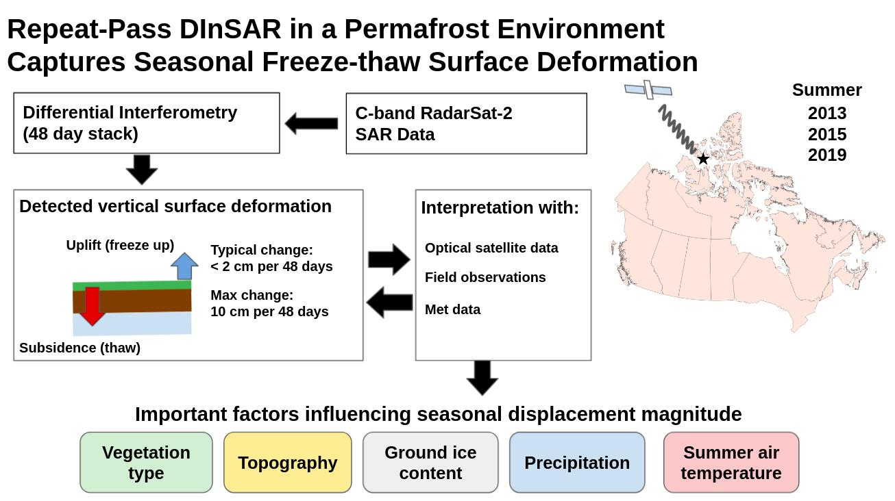
2.1. Overview
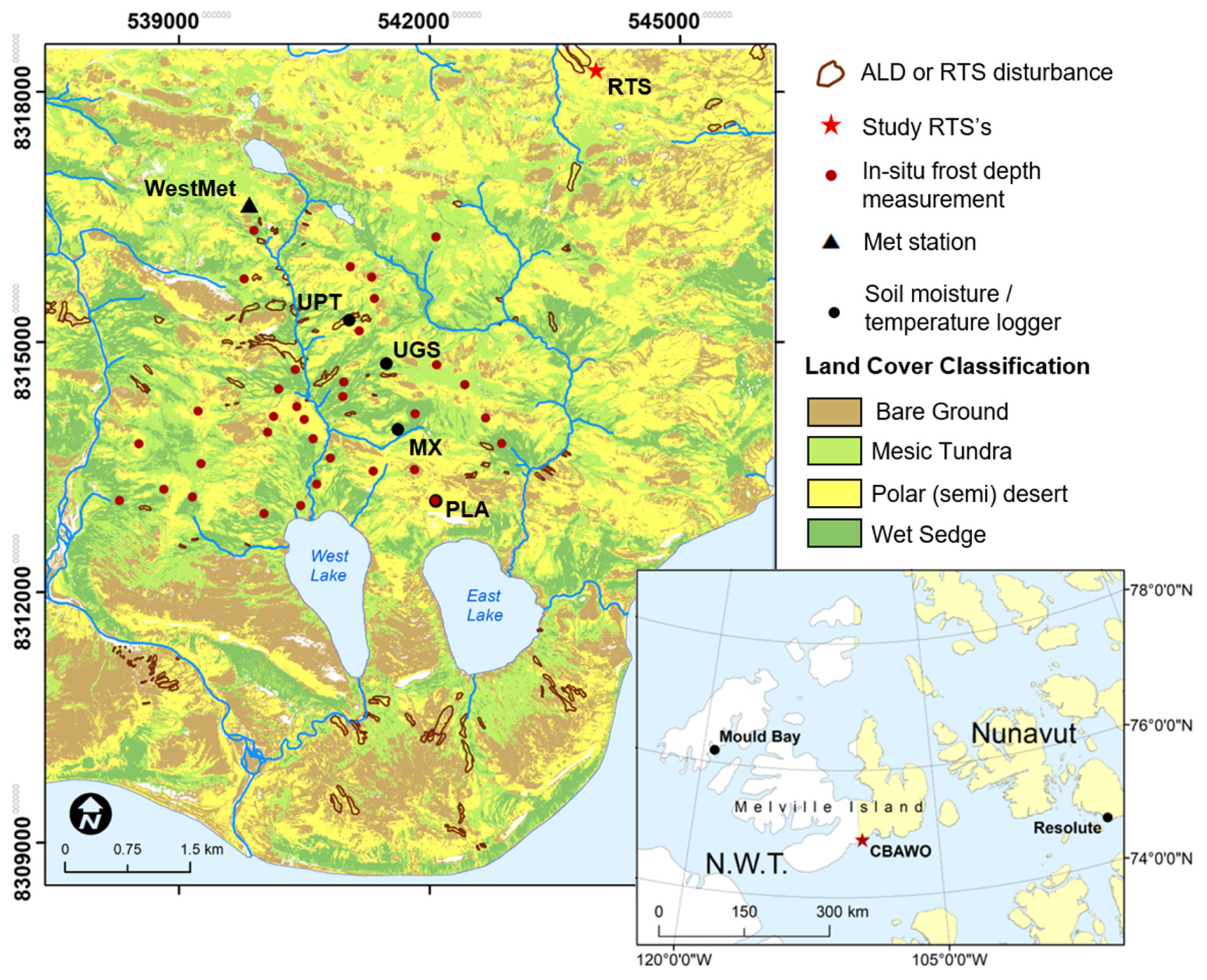
2.2. Study Area
2.3. Field Measurements: Frost Depth, Soil Moisture, and Meteorological Data
2.4. Optical Satellite Data
2.5. Wetness Indices
2.6. SAR Imagery
2.7. DInSAR Processing
2.8. Derivation of Metrics to Characterize Long-Term Spatial Patterns of Displacement (2013-19)
3. Analysis
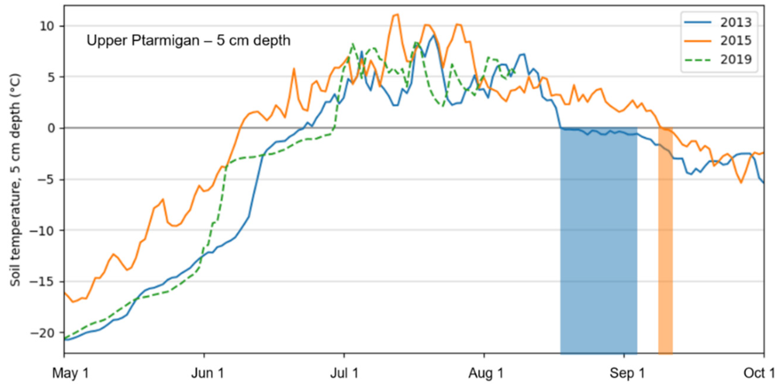
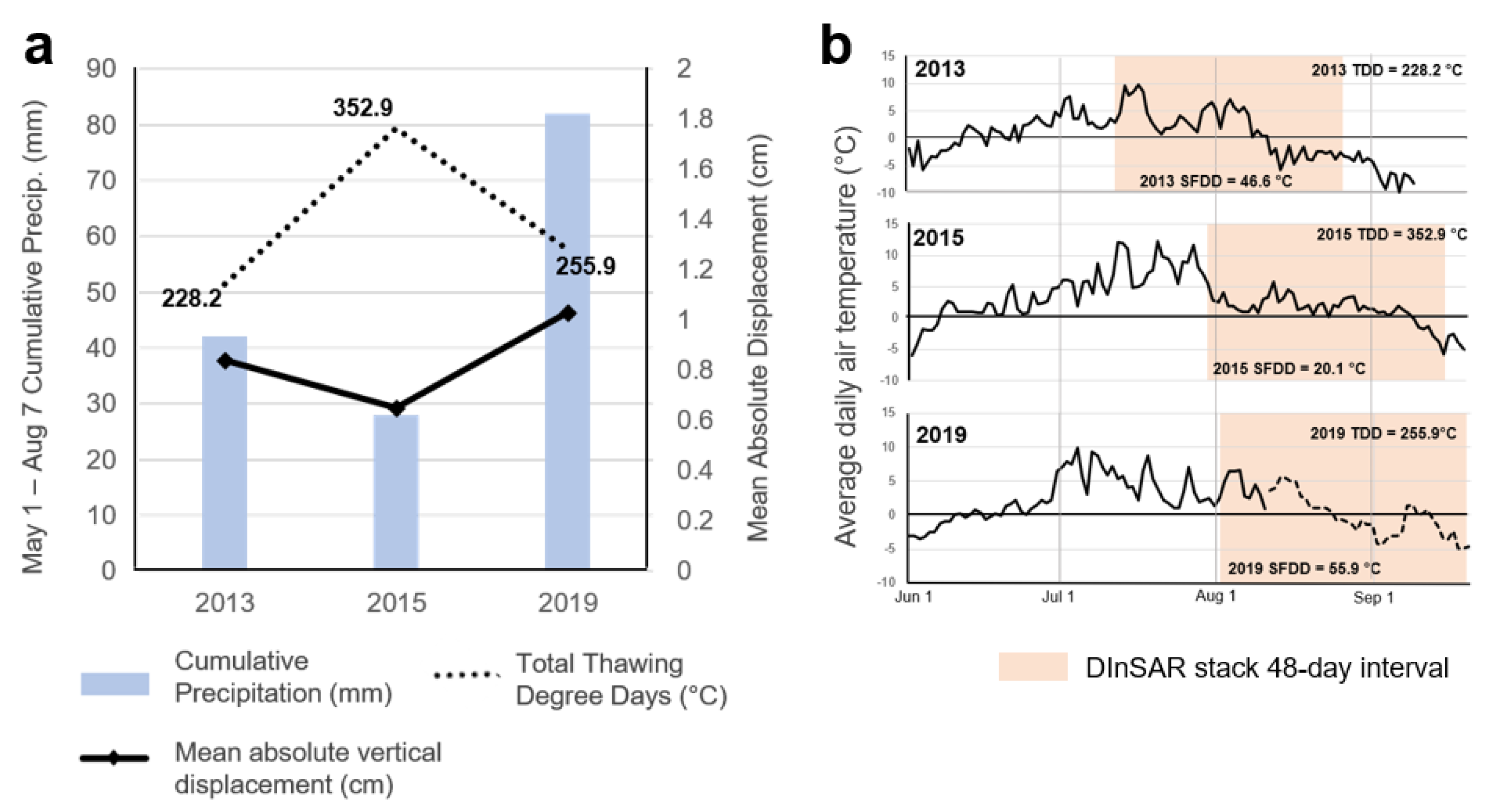
3.1. Meteorological and Soil Conditions
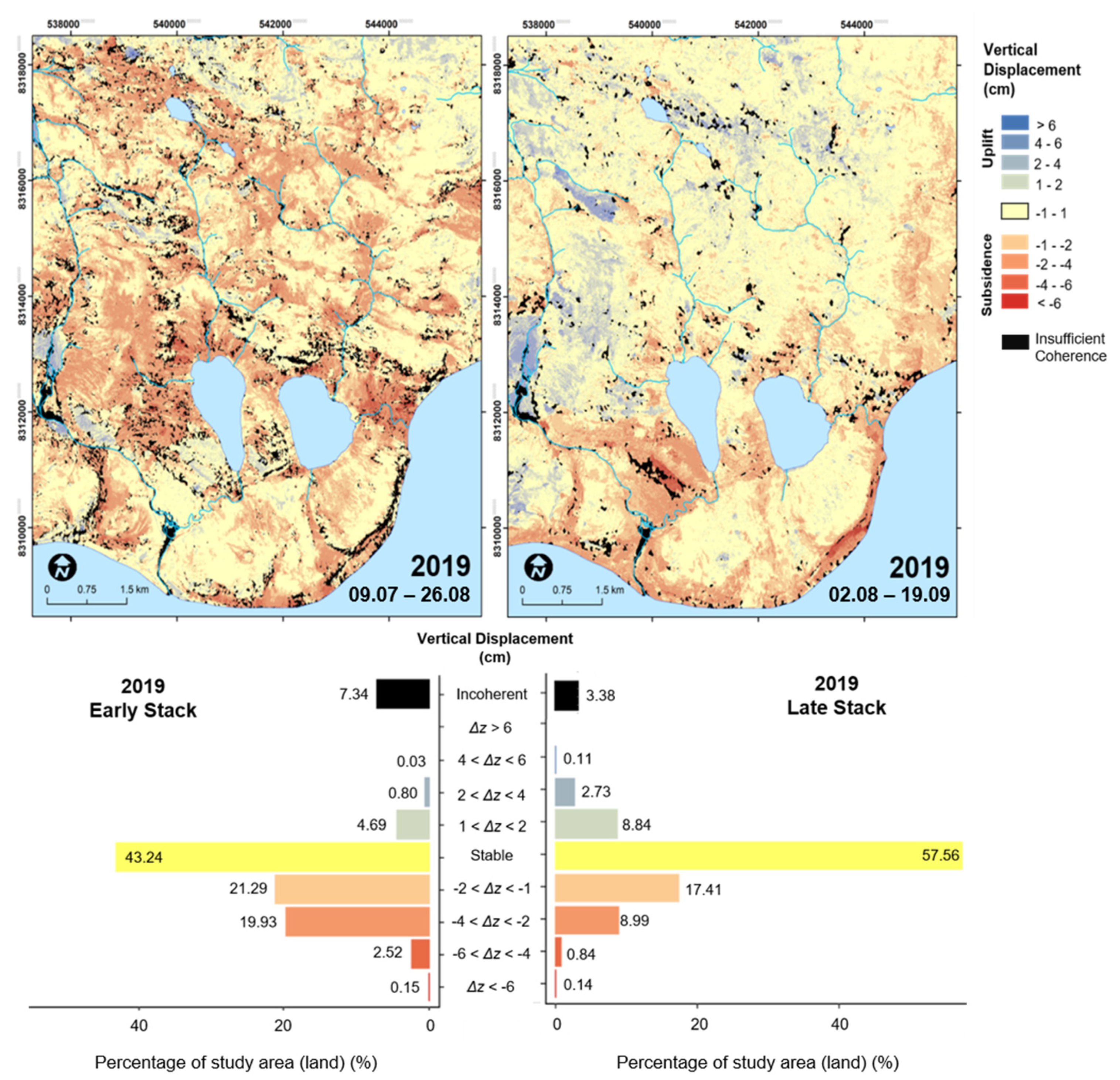
3.2. Early versus Late-Season Displacement (2019)
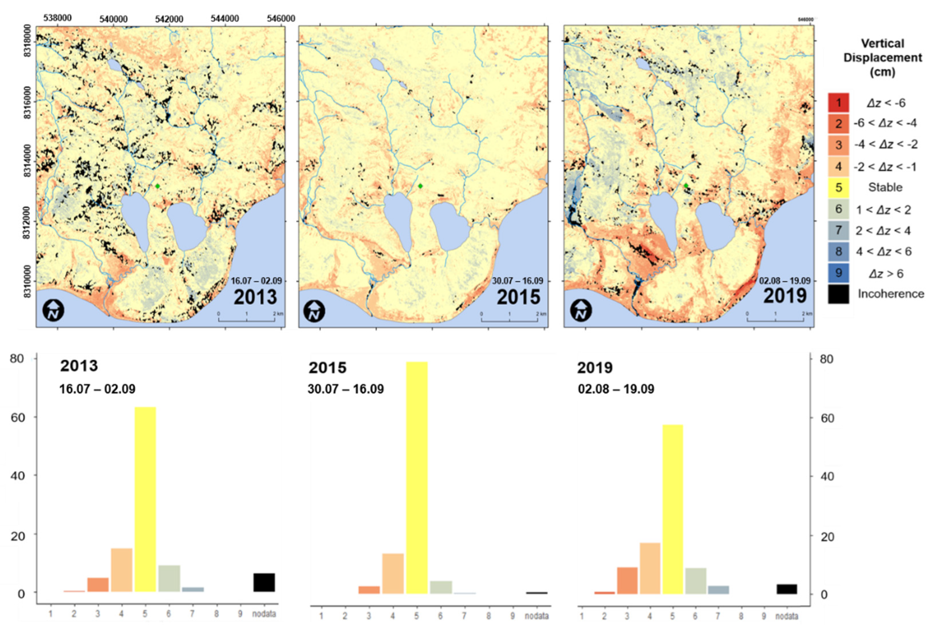
3.3. Comparison of Single-Season Displacement Maps (2013, 2015, 2019)
3.4. Displacement Maps in Relation to Environmental and Topographic Variables
3.4.1. Land-Cover Type
3.4.2. Topographic Wetness Index
3.4.3. Slope Angle
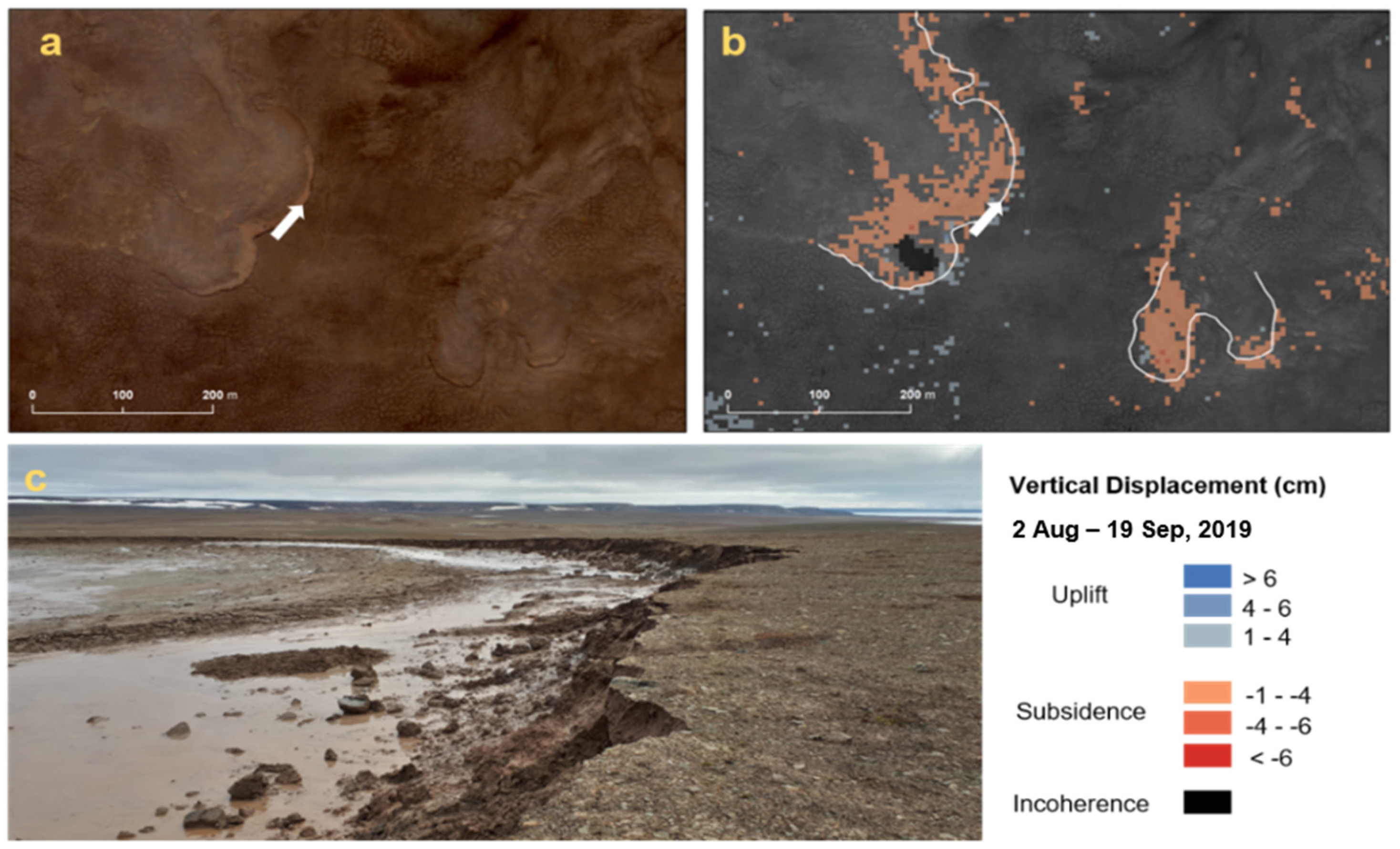
3.5. Surface Displacement Related to Landscape Features
3.6. Metrics to Characterize Spatial Patterns of Displacement over Multiple Summers (2013-19)
3.6.1. Assessing Frequency of Displacement
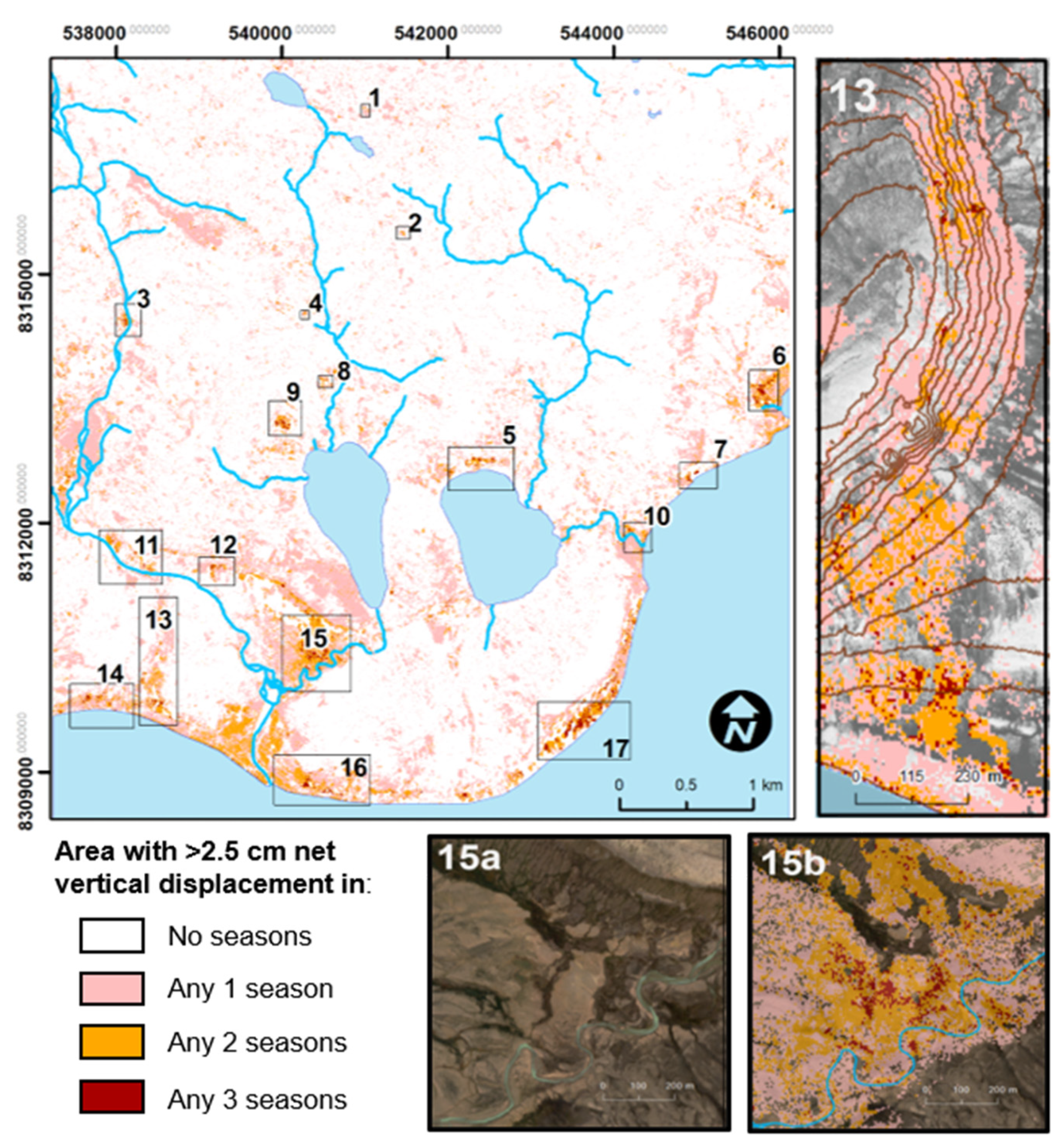
3.6.2. Assessing Aggregate Displacement of Multiple Individual Seasonal Maps
5. Conclusions
Supplementary Materials
Author Contributions
Funding
Data Availability Statement
Acknowledgments
Conflicts of Interest
References
- Chadburn, S.E.; Burke, E.J.; Cox, P.M.; Friedlingstein, P.; Hugelius, G.; Westermann, S. An observation-based constraint on permafrost loss as a function of global warming. Nat. Clim. Chang. 2017, 7, 340–344. [Google Scholar] [CrossRef]
- French, H.M. The Periglacial Environment, 3rd ed.; Wiley: Hoboken, NJ, USA, 2007. [Google Scholar]
- Lewkowicz, A.G. Dynamics of active-layer detachment failures, Fosheim peninsula, Ellesmere Island, Nunavut, Canada. Permafr. Periglac. Process. 2007, 18, 89–103. [Google Scholar] [CrossRef]
- Burn, C.R. The thermal regime of a retrogressive thaw slump near Mayo, Yukon Territory. Can. J. Earth Sci. 2000, 37, 967–981. [Google Scholar] [CrossRef]
- Kokelj, S.V.; Jorgenson, M.T. Advances in thermokarst research. Permafr. Periglac. Process. 2013, 24, 108–119. [Google Scholar] [CrossRef]
- Shiklomanov, N.I.; Streletskiy, D.A.; Little, J.D.; Nelson, F.E. Isotropic thaw subsidence in undisturbed permafrost landscapes. Geophys. Res. Lett. 2013, 40, 6356–6361. [Google Scholar] [CrossRef]
- Liu, L.; Zhang, T.; Wahr, J. InSAR measurements of surface deformation over permafrost on the North Slope of Alaska. J. Geophys. Res. Earth Surf. 2010, 115, F0324. [Google Scholar] [CrossRef]
- Ballantyne, C.B. Periglacial Geomorphology; Wiley: Hoboken, NJ, USA, 2018. [Google Scholar]
- Hauck, C.; Böttcher, M.; Maurer, H. A new model for estimating subsurface ice content based on combined electrical and seismic data sets. Cryosphere 2011, 5, 453–468. [Google Scholar] [CrossRef] [Green Version]
- O’Neill, H.B.; Wolfe, S.A.; Duchesne, C. New ground ice maps for Canada using a paleogeographic modelling approach. Cryosphere 2019, 13, 753–773. [Google Scholar] [CrossRef] [Green Version]
- Lewkowicz, A.G.; Harris, C. Frequency and magnitude of active-layer detachment failures in discontinuous and continuous permafrost, northern Canada. Permafr. Periglac. Process. 2005, 16, 115–130. [Google Scholar] [CrossRef]
- Antonova, S.; Sudhaus, H.; Strozzi, T.; Zwieback, S.; Kääb, A.; Heim, B.; Langer, M.; Bornemann, N.; Boike, J. Thaw subsidence of a Yedoma landscape in northern Siberia, measured in situ and estimated from TerraSAR-X interferometry. Remote Sens. 2018, 10, 494. [Google Scholar] [CrossRef] [Green Version]
- Fortier, D.; Allard, M. Frost-cracking conditions, Bylot Island, eastern Canadian Arctic Archipelago. Permafr. Periglac. Process. 2005, 16, 145–161. [Google Scholar] [CrossRef]
- Otto, J.C.; Keuschnig, M.; Götz, J.; Marbach, M.; Schrott, L. Detection of mountain permafrost by combining high resolution surface and subsurface information–an example from the Glatzbach catchment, Austrian Alps. Geogr. Ann. Ser. A Phys. Geogr. 2012, 94, 43–57. [Google Scholar] [CrossRef]
- Bartsch, A.; Leibman, M.; Strozzi, T.; Khomutov, A.; Widhalm, B.; Babkina, E.; Mullanurov, D.; Ermokhina, K.; Kroisleitner, C.; Bergstedt, H. Seasonal Progression of Ground Displacement Identified with Satellite Radar Interferometry and the Impact of Unusually Warm Conditions on Permafrost at the Yamal Peninsula in 2016. Remote Sens. 2019, 11, 1865. [Google Scholar] [CrossRef] [Green Version]
- Rouyet, L.; Lauknes, T.R.; Christiansen, H.H.; Strand, S.M.; Larsen, Y. Seasonal dynamics of a permafrost landscape, Adventdalen, Svalbard, investigated by InSAR. Remote Sens. Environ. 2019, 231, 111236. [Google Scholar] [CrossRef]
- Zhao, R.; Li, Z.W.; Feng, G.C.; Wang, Q.J.; Hu, J. Monitoring surface deformation over permafrost with an improved SBAS-InSAR algorithm: With emphasis on climatic factors modeling. Remote Sens. Environ. 2016, 184, 276–287. [Google Scholar] [CrossRef]
- Raynolds, M.K.; Walker, D.A. Circumpolar relationships between permafrost characteristics, NDVI, and Arctic vegetation types. In Proceedings of the Ninth International Conference on Permafrost (NICOP 2008), Fairbanks, AK, USA, 29 June–3 July 2008; Volume 2, pp. 1469–1474. [Google Scholar]
- Gruber, S. Ground subsidence and heave over permafrost: Hourly time series reveal inter-annual, seasonal and shorter-term movement caused by freezing, thawing and water move-ment. Cryosphere 2020, 14, 1437–1447. [Google Scholar] [CrossRef]
- Shur, Y.; Hinkel, K.M.; Nelson, F.E. The transient layer: Implications for geocryology and climate-change science. Permafr. Periglac. Process. 2005, 16, 5–17. [Google Scholar] [CrossRef]
- Lamoureux, S.F.; Lafrenière, M.J. Fluvial impact of extensive active layer detachments, Cape Bounty, Melville Island, Canada. Arct. Antarct. Alp. Res. 2009, 41, 59–68. [Google Scholar] [CrossRef]
- Nelson, F.E.; Anisimov, O.A.; Shiklomanov, N.I. Subsidence risk from thawing permafrost. Nature 2001, 410, 889–890. [Google Scholar] [CrossRef]
- Koven, C.D.; Ringeval, B.; Friedlingstein, P.; Ciais, P.; Cadule, P.; Khvorostyanov, D.; Krinner, G.; Tarnocai, C. Permafrost carbon-climate feedbacks accelerate global warming. Proc. Natl. Acad. Sci. USA 2011, 108, 14769–14774. [Google Scholar] [CrossRef] [Green Version]
- Romanovsky, V.E.; Marchenko, S.S.; Daanen, R.; Sergeev, D.O.; Walker, D.A. Soil climate and frost heave along the permafrost/ecological North American Arctic transect. In Proceedings of the Ninth International Conference on Permafrost; Institute of Northern Engineering: Fairbanks, AK, USA, 2008; Volume 2, pp. 1519–1524. [Google Scholar]
- Little, J.D.; Sandall, H.; Walegur, M.T.; Nelson, F.E. Application of differential global positioning systems to monitor frost heave and thaw settlement in tundra environments. Permafr. Periglac. Process. 2003, 14, 349–357. [Google Scholar] [CrossRef]
- Avian, M.; Kellerer-Pirklbauer, A.; Bauer, A. LiDAR for monitoring mass movements in permafrost environments at the cirque Hinteres Langtal, Austria, between 2000 and 2008. Nat. Hazards Earth Syst. Sci. 2009, 9, 1087–1094. [Google Scholar] [CrossRef]
- Kääb, A.; Girod, L.M.R.; Berthling, I.T. Surface kinematics of periglacial sorted circles using structure-from-motion technology. Cryosphere 2014, 8, 1041–1056. [Google Scholar] [CrossRef] [Green Version]
- Gabriel, A.K.; Goldstein, R.M.; Zebker, H.A. Mapping small elevation changes over large areas: Differential radar interferometry. J. Geophys. Res. Solid Earth 1989, 94, 9183–9191. [Google Scholar] [CrossRef]
- Zwieback, S.; Liu, X.; Antonova, S.; Heim, B.; Bartsch, A.; Boike, J.; Hajnsek, I. A statistical test of phase closure to detect influences on DInSAR deformation estimates besides displacements and decorrelation noise: Two case studies in high-latitude regions. IEEE Trans. Geosci. Remote Sens. 2016, 54, 5588–5601. [Google Scholar] [CrossRef]
- Strozzi, T.; Antonova, S.; Günther, F.; Mätzler, E.; Vieira, G.; Wegmüller, U.; Westermann, S.; Bartsch, A. Sentinel-1 SAR interferometry for surface deformation monitoring in low-land permafrost areas. Remote Sens. 2018, 10, 1360. [Google Scholar] [CrossRef] [Green Version]
- Khalil, R.Z.; ul-Haque, S. InSAR coherence-based land cover classification of Okara, Pakistan. Egypt. J. Remote Sens. Space Sci. 2018, 21, S23–S28. [Google Scholar] [CrossRef]
- Zhang, T.; Barry, R.G.; Armstrong, R.L. Application of satellite remote sensing techniques to frozen ground studies. Polar Geogr. 2004, 28, 163–196. [Google Scholar] [CrossRef]
- Short, N.; Brisco, B.; Couture, N.; Pollard, W.; Murnaghan, K.; Budkewitsch, P. A comparison of TerraSAR-X, RADARSAT-2 and ALOS-PALSAR interferometry for monitoring permafrost environments, case study from Herschel Island, Canada. Remote Sens. Environ. 2011, 115, 3491–3506. [Google Scholar] [CrossRef]
- Rudy, A.C.; Lamoureux, S.F.; Treitz, P.; Short, N.; Brisco, B. Seasonal and multi-year surface displacements measured by DInSAR in a High Arctic permafrost environment. Int. J. Appl. Earth Obs. Geoinf. 2018, 64, 51–61. [Google Scholar] [CrossRef]
- Bernhard, P.; Zwieback, S.; Leinss, S.; Hajnsek, I. Mapping Retrogressive Thaw Slumps Using Single-Pass TanDEM-X Observations. IEEE J. Sel. Top. Appl. Earth Obs. Remote Sens. 2020, 13, 3263–3280. [Google Scholar] [CrossRef]
- Chen, L.M.; Qiao, G.; Lu, P. Surface Deformation Monitoring in Permafrost Regions of Tibetan Plateau Based on ALOS PALSAR Data. The International Archives of Photogrammetry. Remote Sens. Spat. Inf. Sci. 2017, 42, 1509–1512. [Google Scholar]
- Daout, S.; Doin, M.P.; Peltzer, G.; Socquet, A.; Lasserre, C. Large-scale InSAR monitoring of permafrost freeze-thaw cycles on the Tibetan Plateau. Geophys. Res. Lett. 2017, 44, 901–909. [Google Scholar] [CrossRef]
- Lu, P.; Han, J.; Hao, T.; Li, R.; Qiao, G. Seasonal deformation of permafrost in Wudaoliang basin in Qinghai-Tibet plateau revealed by StaMPS-InSAR. Mar. Geodesy 2020, 43, 248–268. [Google Scholar] [CrossRef]
- Wolfe, S.A.; Short, N.H.; Morse, P.D.; Schwarz, S.H.; Stevens, C.W. Evaluation of RADARSAT-2 DInSAR seasonal surface displacement in discontinuous permafrost terrain, Yellowknife, Northwest Territories, Canada. Can. J. Remote Sens. 2014, 40, 406–422. [Google Scholar] [CrossRef]
- LeBlanc, A.M.; Short, N.; Mathon-Dufour, V.; Allard, M.; Tremblay, T.; Oldenborger, G.A.; Chartrand, J. DInSAR seasonal surface displacement in built and natural permafrost environments, Iqaluit, Nunavut, Canada. In Proceedings of the GEO, Québec, QC, Canada, 20–23 September 2015; pp. 20–23. [Google Scholar]
- Zwieback, S.; Meyer, F.J. Top-of-permafrost ground ice indicated by remotely sensed late-season disturbance. Cryosphere 2021, 15, 2041–2055. [Google Scholar] [CrossRef]
- Hung, J.K.Y.; Treitz, P. Environmental land-cover classification for integrated watershed studies: Cape Bounty, Melville Island, Nunavut. Arct. Sci. 2020, 6, 404–422. [Google Scholar] [CrossRef]
- Bonnaventure, P.P.; Lamoureux, S.F.; Favaro, E.A. Over-Winter Channel Bed Temperature Regimes Generated by Contrasting Snow Accumulation in a High Arctic River. Permafr. Periglac. Process. 2016, 28, 339–346. [Google Scholar] [CrossRef] [Green Version]
- Atkinson, D.M.; Treitz, P. Arctic ecological classifications derived from vegetation community and satellite spectral data. Remote Sens. 2012, 4, 3948–3971. [Google Scholar] [CrossRef] [Green Version]
- Lamoureux, S.F.; Lafrenière, M.J. More than just snowmelt: Integrated watershed science for changing climate and permafrost at the Cape Bounty Arctic Watershed Observatory. Wiley Interdiscip. Rev. Water 2017, 5, e1255. [Google Scholar] [CrossRef]
- Paquette, M.; Rudy, A.C.; Fortier, D.; Lamoureux, S.F. Multi-scale site evaluation of a relict active layer detachment in a High Arctic landscape. Geomorphology 2020, 359, 107159. [Google Scholar] [CrossRef]
- Collingwood, A.; Treitz, P.; Charbonneau, F. Surface roughness estimation from RADARSAT-2 data in a High Arctic environment. Int. J. Appl. Earth Obs. Geoinf. 2014, 27, 70–80. [Google Scholar] [CrossRef]
- Rudy, A.C.; Lamoureux, S.F.; Treitz, P.; Collingwood, A. Identifying permafrost slope disturbance using multi-temporal optical satellite images and change detection techniques. Cold Reg. Sci. Technol. 2013, 88, 37–49. [Google Scholar] [CrossRef]
- Shoshany, M.; Svoray, T.; Curran, P.J.; Foody, G.M.; Perevolotsky, A. The relationship between ERS-2 SAR backscatter and soil moisture: Generalization from a humid to semi-arid transect. Int. J. Remote. Sens. 2000, 21, 2337–2343. [Google Scholar] [CrossRef]
- Collingwood, A.; Shang, C.; Charbonneau, F.; Treitz, P. Spatiotemporal variability of Arctic soil moisture detected from high-resolution RADARSAT-2 SAR data. Adv. Meteorol. 2018. [Google Scholar] [CrossRef]
- Crosson, W.L.; Laymon, C.A.; Inguva, R.; Schamschula, M.P. Assimilating remote sensing data in a surface flux–soil moisture model. Hydrol. Process. 2002, 16, 1645–1662. [Google Scholar] [CrossRef]
- Roberts, K.E.; Lamoureux, S.F.; Kyser, T.K.; Muir, D.C.G.; Lafrenière, M.J.; Iqaluk, D.; Pieńkowski, A.J.; Normandeau, A. Climate and permafrost effects on the chemistry and ecosystems of High Arctic Lakes. Sci. Rep. 2017, 7, 1–8. [Google Scholar] [CrossRef] [Green Version]
- Boyd, D.W. Normal freezing and thawing degree-days from normal monthly temperatures. Can. Geotech. J. 1976, 13, 176–180. [Google Scholar] [CrossRef]
- ArcMap, Version 10.7.1 [Software]; ESRI: Redlands, CA, USA, 2019.
- Kuester, M. Technical Note: Radiometric Use of WorldView-3 Imagery; DigitalGlobe: Longmont, CO, USA, 2016. [Google Scholar]
- Kokelj, S.V.; Tunnicliffe, J.; Lacelle, D.; Lantz, T.C.; Chin, K.S.; Fraser, R. Increased precipitation drives mega slump development and destabilization of ice-rich permafrost terrain, northwestern Canada. Glob. Planet. Chang. 2015, 129, 56–68. [Google Scholar] [CrossRef] [Green Version]
- Yarbrough, L.D.; Navulur, K.; Ravi, R. Presentation of the Kauth–Thomas transform for WorldView-2 reflectance data. Remote Sens. Lett. 2014, 5, 131–138. [Google Scholar] [CrossRef]
- Kauth, R.J.; Thomas, G.S. The tasselled cap–a graphic description of the spectral-temporal development of agricultural crops as seen by Landsat. In LARS Symposia; Purdue University: West Lafayette, IN, USA, 1976; pp. 159–170. [Google Scholar]
- Sørensen, R.; Zinko, U.; Seibert, J. On the calculation of the topographic wetness index: Evaluation of different methods based on field observations. Hydrol. Earth Syst. Sci. 2006, 10, 101–112. [Google Scholar] [CrossRef] [Green Version]
- Lindsay, J.B. Whitebox GAT: A case study in geomorphometric analysis. Comput. Geosci. 2016, 95, 75–84. [Google Scholar] [CrossRef]
- Eppler, J.; Kubanski, M.; Sharma, J.; Busler, J. High temporal resolution permafrost monitoring using a multiple stack InSAR technique. The International Archives of Photogrammetry. Remote Sens. Spat. Inf. Sci. 2015, 40, 1171–1177. [Google Scholar]
- Sandwell, D.T.; Myer, D.; Mellors, R.; Shimada, M.; Brooks, B.; Foster, J. Accuracy and resolution of ALOS interferometry: Vector deformation maps of the Father’s Day intrusion at Kilauea. IEEE Trans. Geosci. Remote Sens. 2008, 46, 3524–3534. [Google Scholar] [CrossRef] [Green Version]
- Werner, C.; Wegmüller, U.; Strozzi, T.; Wiesmann, A. Processing strategies for phase unwrapping for INSAR applications. In Proceedings of the European Conference on Synthetic Aperture Radar (EUSAR 2002), Cologne, Germany, 4–6 June 2002; Volume 1, pp. 353–356. [Google Scholar]
- Porter, C.; Morin, P.; Howat, I.; Noh, M.-J.; Bates, B.; Peterman, K.; Keesey, S.; Schlenk, M.; Gardiner, J.; Tomko, K.; et al. ArcticDEM, Harvard Dataverse, V1. 2018. Available online: https://0-doi-org.brum.beds.ac.uk/10.7910/DVN/OHHUKH (accessed on 26 November 2019).
- Moreira, A. Improved multilook techniques applied to SAR and SCANSAR imagery. IEEE Trans. Geosci. Remote Sens. 1991, 29, 529–534. [Google Scholar] [CrossRef]
- Kumar, V.; Venkataraman, G. SAR interferometric coherence analysis for snow cover mapping in the western Himalayan region. Int. J. Digit. Earth 2011, 4, 78–90. [Google Scholar] [CrossRef]
- Outcalt, S.I.; Nelson, F.E.; Hinkel, K.M. The zero-curtain effect: Heat and mass transfer across an isothermal region in freezing soil. Water Resour. Res. 1990, 26, 1509–1516. [Google Scholar]
- Stieglitz, M.; Déry, S.J.; Romanovsky, V.E.; Osterkamp, T.E. The role of snow cover in the warming of arctic permafrost. Geophys. Res. Lett. 2003, 30, 1721–1725. [Google Scholar] [CrossRef]
- Farquharson, L.M.; Mann, D.H.; Grosse, G.; Jones, B.M.; Romanovsky, V.E. Spatial distribution of thermokarst terrain in Arctic Alaska. Geomorphology 2016, 273, 116–133. [Google Scholar] [CrossRef] [Green Version]
- Nolan, M.; Fatland, D.R. Penetration depth as a DInSAR observable and proxy for soil moisture. IEEE Trans. Geosci. Remote Sens. 2003, 41, 532–537. [Google Scholar] [CrossRef] [Green Version]
- McFadden, S.I. Fine Scale Ground Surface and Vertical Displacement and Soil Water Processes in the Canadian High Arctic. Master’s Thesis, Queen’s University, Kingston, ON, Canada, 2019. Available online: http://hdl.handle.net/1974/26313 (accessed on 1 November 2020).
- Short, N.; LeBlanc, A.M.; Sladen, W.; Brisco, B. RADARSAT-2 InSAR for monitoring permafrost environments: Pangnirtung and Iqaluit. In Proceedings of the 2013 IEEE Radar Conference (RadarCon13), Ottawa, ON, Canada, 29 April–3 May 2013; pp. 1–4. [Google Scholar]
- Verpaelst, M.; Fortier, D.; Kanevskiy, M.; Paquette, M.; Shur, Y. Syngenetic dynamic of permafrost of a polar desert solifluction lobe, Ward Hunt Island, Nunavut. Arct. Sci. 2017, 3, 301–319. [Google Scholar] [CrossRef] [Green Version]
- Hu, B.; Wu, Y.; Zhang, X.; Yang, B.; Chen, J.; Li, H.; Chen, X.; Chen, Z. Monitoring the Thaw Slump-Derived Thermokarst in the Qinghai-Tibet Plateau Using Satellite SAR Interferometry. J. Sens. 2019, 2019, 1698432. [Google Scholar] [CrossRef]
- Burn, C.R.; Lewkowicz, A.G. Canadian landform examples-17 retrogressive thaw slumps. Can. Geogr. 1990, 34, 273–276. [Google Scholar] [CrossRef]
- Lantz, T.C.; Kokelj, S.V. Increasing rates of retrogressive thaw slump activity in the Mackenzie Delta region, NWT, Canada. Geophys. Res. Lett. 2008, 35, L06502. [Google Scholar] [CrossRef]
- Ramage, J.L.; Irrgang, A.; Morgenstern, A.; Lantuit, H. Contribution of Coastal Retrogressive Thaw Slumps to the Nearshore Organic Carbon budget along the Yukon Coast. Biogeosci. Discuss. 2017. [Google Scholar] [CrossRef] [Green Version]
- Lajeunesse, P.; Hanson, M.A. Field observations of recent transgression on northern and eastern Melville Island, western Canadian Arctic Archipelago. Geomorphology 2008, 101, 618–630. [Google Scholar] [CrossRef]
- England, J.H.; Furze, M.F.; Doupé, J.P. Revision of the NW Laurentide Ice Sheet: Implications for paleoclimate, the northeast extremity of Beringia, and Arctic Ocean sedimentation. Quat. Sci. Rev. 2009, 28, 1573–1596. [Google Scholar] [CrossRef]
- Holloway, J.E.; Lamoureux, S.F.; Montross, S.N.; Lafrenière, M.J. Climate and terrain characteristics linked to mud ejection occurrence in the Canadian High Arctic. Permafr. Periglac. Process. 2016, 27, 204–218. [Google Scholar] [CrossRef] [Green Version]
- Rudy, A.C.; Lamoureux, S.F.; Treitz, P.; Ewijk, K.V.; Bonnaventure, P.P.; Budkewitsch, P. Terrain Controls and Landscape-Scale Susceptibility Modelling of Active-Layer Detachments, Sabine Peninsula, Melville Island, Nunavut. Permafr. Periglac. Process. 2017, 28, 79–91. [Google Scholar] [CrossRef] [Green Version]


| Year | Stack Dates | Pairs Used | Temporal Baseline (days) |
|---|---|---|---|
| 2013 | 16 July–2 September | 16 July–9 August 9 August–2 September | 24 24 |
| 2015 | 30 July–16 September | 30 July–23 August 23 August–16 September | 24 24 |
| 2019 | 9 July–26 August | 9 July–2 August 2 –26 August | 24 24 |
| 2019 | 2 August–19 September | 2 –26 August 26 August–19 September | 24 24 |
| Land-Cover Type | TWI | Slope | |||||||||
|---|---|---|---|---|---|---|---|---|---|---|---|
| Summer Stack | Bare Ground | Mesic Tundra | Polar (semi) Desert | Wet Sedge | Low | Med | High | <2° | 2–5° | 5–8° | >8° |
| 2013 | 0.9 | 1.3 | 0.5 | 3.1 | 3.2 | 2.2 | 2.6 | 2.4 | 2.8 | 3.0 | 3.1 |
| 2015 | 0.2 | 0.2 | 0.1 | 2.0 | 1.1 | 1.0 | 1.2 | 0.8 | 1.0 | 1.3 | 2.3 |
| 2019 | 3.9 | 2.1 | 2.4 | 7.1 | 7.2 | 6.8 | 6.2 | 4.1 | 5.3 | 7.6 | 19.8 |
| Mean Vertical Surface Displacement inside and outside Mapped Disturbances (cm) | Mean Absolute Vertical Surface Displacement inside and outside Mapped Disturbances (cm) | |||||
|---|---|---|---|---|---|---|
| Period | Outside | Inside | t-Test | Outside | Inside | t-Test |
| 16 July–2 September 2013 | −0.06 | −0.35 | t = −12.79, p < 0.001 | 0.79 | 0.85 | t = 3.14, p = 0.002 |
| 30 July–16 September 2015 | −0.12 | −0.29 | t = −7.27, p < 0.001 | 0.57 | 0.63 | t = 4.14, p < 0.001 |
| 2 August–19 September 2019 | −0.42 | −0.85 | t= −14.95, p < 0.001 | 0.83 | 1.02 | t = 9.27, p < 0.001 |
| Net Vertical Subsidence (>2.5 cm) (%) | Net Vertical Uplift (>2.5 cm) (%) | Subsidence One Year, Uplift in Another (%) | No change >±2.5 cm Observed (%) | ||||
|---|---|---|---|---|---|---|---|
| 1 Season | 2 Seasons | 3 Seasons | 1 Season | 2 Seasons | 3 Seasons | ||
| 6.18 | 0.89 | 0.06 | 1.93 | 0.02 | <0.01 | 0.06 | 90.87 |
| Mean Value in Each Frequency Zone (Years Where >2.5 cm Displacement Occurred) | ||||||
|---|---|---|---|---|---|---|
| Variable | Stat. Test | Test Result | 0 | 1 | 2 | 3 |
| Wetness (Spectral) | ANOVA | F = 7.98, p < 0.001 * | −1.23 | −1.28 | −1.34 | −1.29 |
| Wetness (TWI) | ANOVA | F = 0.94, p = 0.423 | 6.10 | 6.02 | 6.21 | 6.08 |
| Slope | ANOVA | F = 39.5, p < 0.001 * | 5.80 | 8.78 | 8.10 | 9.72 |
| Elevation | ANOVA | F = 525.0, p < 0.001 * | 64.15 | 48.81 | 23.76 | 18.42 |
| Land-cover class | Chi-Squared | χ2 = 570.8, p < 0.001 * | N/A | N/A | N/A | N/A |
Publisher’s Note: MDPI stays neutral with regard to jurisdictional claims in published maps and institutional affiliations. |
© 2021 by the authors. Licensee MDPI, Basel, Switzerland. This article is an open access article distributed under the terms and conditions of the Creative Commons Attribution (CC BY) license (https://creativecommons.org/licenses/by/4.0/).
Share and Cite
Robson, G.; Treitz, P.; Lamoureux, S.F.; Murnaghan, K.; Brisco, B. Seasonal Surface Subsidence and Frost Heave Detected by C-Band DInSAR in a High Arctic Environment, Cape Bounty, Melville Island, Nunavut, Canada. Remote Sens. 2021, 13, 2505. https://0-doi-org.brum.beds.ac.uk/10.3390/rs13132505
Robson G, Treitz P, Lamoureux SF, Murnaghan K, Brisco B. Seasonal Surface Subsidence and Frost Heave Detected by C-Band DInSAR in a High Arctic Environment, Cape Bounty, Melville Island, Nunavut, Canada. Remote Sensing. 2021; 13(13):2505. https://0-doi-org.brum.beds.ac.uk/10.3390/rs13132505
Chicago/Turabian StyleRobson, Greg, Paul Treitz, Scott F. Lamoureux, Kevin Murnaghan, and Brian Brisco. 2021. "Seasonal Surface Subsidence and Frost Heave Detected by C-Band DInSAR in a High Arctic Environment, Cape Bounty, Melville Island, Nunavut, Canada" Remote Sensing 13, no. 13: 2505. https://0-doi-org.brum.beds.ac.uk/10.3390/rs13132505