Article

AlgaeMAp: Algae Bloom Monitoring Application for Inland Waters in Latin America

by
Felipe de Lucia Lobo
1,*,
Gustavo Willy Nagel
2,3,
Daniel Andrade Maciel
2,3,
Lino Augusto Sander de Carvalho
4,
Vitor Souza Martins
5,
Cláudio Clemente Faria Barbosa
3 and
Evlyn Márcia Leão de Moraes Novo
3
1
Center for Technological Development (CDTec), Universidade Federal de Pelotas (UFPel), Pelotas 96010-610, RS, Brazil
2
Remote Sensing Program, Graduate Division, National Institute for Space Research (INPE), São José dos Campos 12227-010, SP, Brazil
3
Instrumentation Lab for Aquatic Systems (LabISA), Earth Observation Coordination of National Institute for Space Research (INPE), São José dos Campos 12227-010, SP, Brazil
4
Department of Meteorology, Federal University of Rio de Janeiro (UFRJ), Rio de Janeiro 21941-916, RJ, Brazil
5
Center for Global Change and Earth Observations, Michigan State University, East Lansing, MI 48824, USA
*
Author to whom correspondence should be addressed.
Remote Sens. 2021, 13(15), 2874; https://0-doi-org.brum.beds.ac.uk/10.3390/rs13152874
Submission received: 27 April 2021 / Revised: 7 July 2021 / Accepted: 20 July 2021 / Published: 22 July 2021
(This article belongs to the Special Issue Remote Sensing of Aquatic Ecosystem Health and Processes)

Abstract

:
Due to increasing algae bloom occurrence and water degradation on a global scale, there is a demand for water quality monitoring systems based on remote sensing imagery. This paper describes the scientific, theoretical, and methodological background for creating a cloud-computing interface on Google Earth Engine (GEE) which allows end-users to access algae bloom related products with high spatial (30 m) and temporal (~5 day) resolution. The proposed methodology uses Sentinel-2 images corrected for atmospheric and sun-glint effects to generate an image collection of the Normalized Difference Chlorophyll-a Index (NDCI) for the entire time-series. NDCI is used to estimate both Chl-a concentration, based on a non-linear fitting model, and Trophic State Index (TSI), based on a tree-decision model classification into five classes. Once the Chl-a and TSI algorithms had been calibrated and validated they were implemented in GEE as an Earth Engine App, entitled Algae Bloom Monitoring Application (AlgaeMAp). AlgaeMAp is the first online platform built within the GEE platform that offers high spatial resolution of water quality parameters. The App benefits from the huge processing capability of GEE that allows any user with internet access to easily extract detailed spatial (30 m) and long temporal Chl-a and TSI information (from August 2015 and with images every 5 days) throughout the most important reservoirs in the State of São Paulo/Brazil. The application will be adapted to extend to other relevant areas in Latin America.

1. Introduction

Human activities on a global scale have significantly contributed to the degradation of the water quality of inland aquatic systems by increasing their nutrient levels. Particularly, reservoirs are under high pressure due to the increasing water demand for urban areas, including irrigation, industrial use, and energy production, while still needing to maintain their ecological function [1,2,3]. The quasi-lentic nature of reservoirs leads to a higher phosphorus accumulation, which may trigger phytoplankton production, abundance, and frequency of algae blooms [4]. Algae bloom (AB) is a rapid increase or accumulation in the population of algae, characterized by the blue-green water coloration caused by algae’s pigments, that can cause serious consequences to human health and aquatic biogeochemistry due to the production of toxins [5,6]. The increase in aquatic ecosystems’ productivity has been monitored by a series of different Trophic State Indexes (TSIs) based on information regarding the nutrient input (generally, phosphorus), water transparency (usually Secchi depth), and chlorophyll concentration (a proxy for phytoplankton biomass) [7]. The advantage of using Chl-a for AB monitoring is that it can be estimated with satellite data and, therefore, used to systematically monitor phytoplankton abundance at a relatively low cost. The interaction between light and photoactive pigments in phytoplankton cells, such as Chlorophyll-a (Chl-a), enables the detection of algae bloom from space-borne imagery [8]. For instance, the Normalized Difference Chlorophyll Index (NDCI) has been used to detect phytoplankton presence by using a ratio of near-infrared (705 nm—maximum phytoplankton reflectance sensitivity) and red bands (665 nm—high Chl-a absorption peak) [9]. In phytoplankton-rich waters around the globe, NDCI has shown to detect a wide Chl-a concentration range when using Sentinel-2 imagery [8,10,11,12]. Watanabe et al. [8] observed that NDCI performed better than other algorithms (2-band, 3-band, and slope) for Chl-a retrieval in the Tietê cascade system, which is the study area of this research.
The development of algorithms using remote sensing for Chl-a estimation relies largely on in situ Chl-a measurements. Unfortunately, the lack of in situ data, in Latin American countries for example, limits water quality management due to the scarce information on the current status of surface waters. This is because most of the monitoring programs provide water quality data at a low frequency (monthly or bi-monthly). Alternatively, the spatial coverage and increased frequency of image acquisition make satellite remote sensing a key tool for AB monitoring programs. Recently, new processing capabilities have used remote sensing historical information, such as Sentinel-2, to track seasonal patterns and degradation tendencies [4,13,14]. The Google Earth Engine (GEE), for instance, offers high performance cloud computing resources to process large amounts of geospatial datasets [15,16]. According to Hirt et al. [17], monitoring water resources using GEE is promising since it offers access to a large image database of several satellites (Sentinel and Landsat programs) thus permitting temporal analysis over large areas. Recent studies have used GEE to map Chl-a concentration and its temporal dynamics [18,19,20,21], showing its ability to monitor phytoplankton abundance and TSI using satellite images.
To meet the need to incorporate satellite remote sensing into the TSI monitoring system in Latin American (LA) inland waters, several researchers from several countries are developing Algae Bloom (AB) mapping tools under the support of GEE and Earth Observation Data Science (EO) [22]. This research aims to develop a user-friendly application (GEE App) to retrieve algae bloom-related products towards a monitoring system for inland waters in Latin America. More specifically, the objective is to calibrate and validate predictive algorithms for Chlorophyll-a and Trophic State Index classes using both in situ data and Sentinel-2/MSI data available in Google Earth Engine. Once parametrized, these predictive algorithms were implemented in the GEE App to compute the spatial and temporal variation of Chl-a concentration and TSI classes. This paper gives the theoretical and methodological background supporting the tool’s development and reports the first results of their application to the monitoring of Tietê River Basin, located in the State of São Paulo, Brazil (Figure 1).

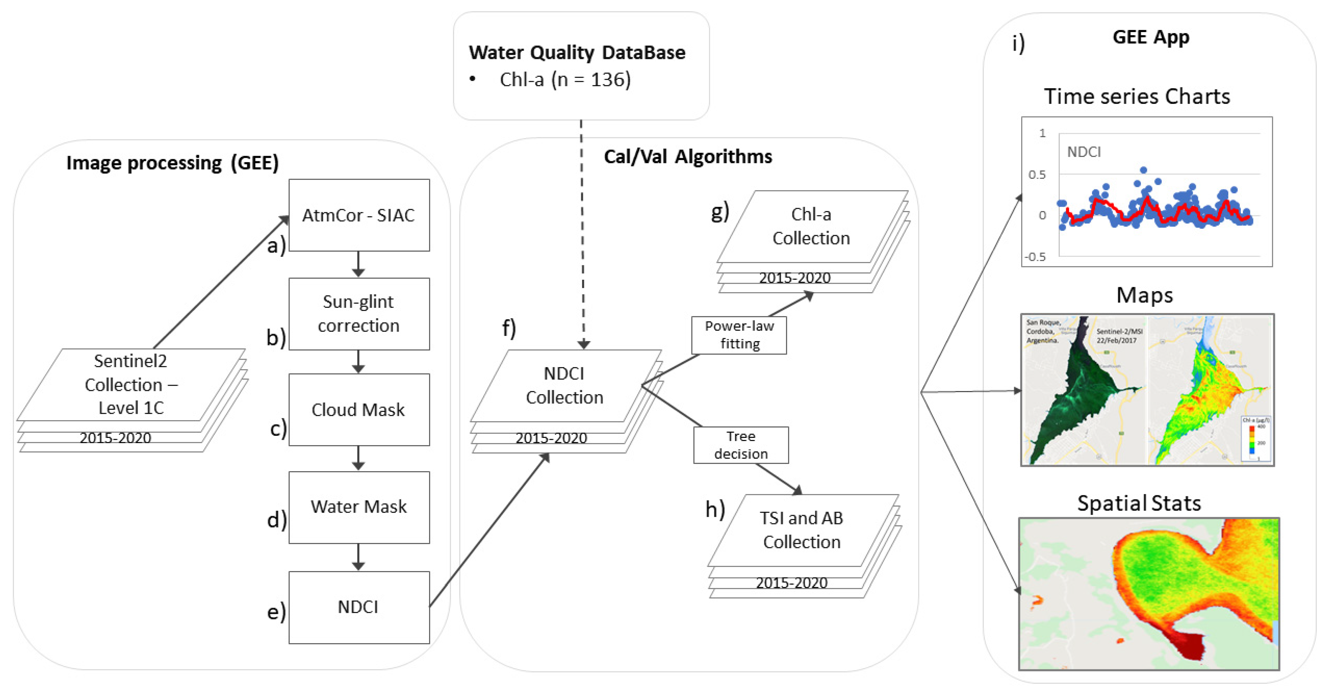
2. Materials and Methods

The proposed methodology uses Sentinel-2 images corrected for atmospheric and sun-glint effects to generate an image collection of the NDCI [9] for the entire time-series (August 2015 to present) of a given area. NDCI data retrieved from the imagery are then compared with Chl-a measured in situ. NDCI is used to estimate both Chl-a concentration, based on a non-linear fitting model, and TSI, based on a tree-decision model. The TSI tree decision classifies every pixel into five levels of Trophic State Index (Oligo, Meso, Eutrophic, Super, and Hypereutrophic) [23].

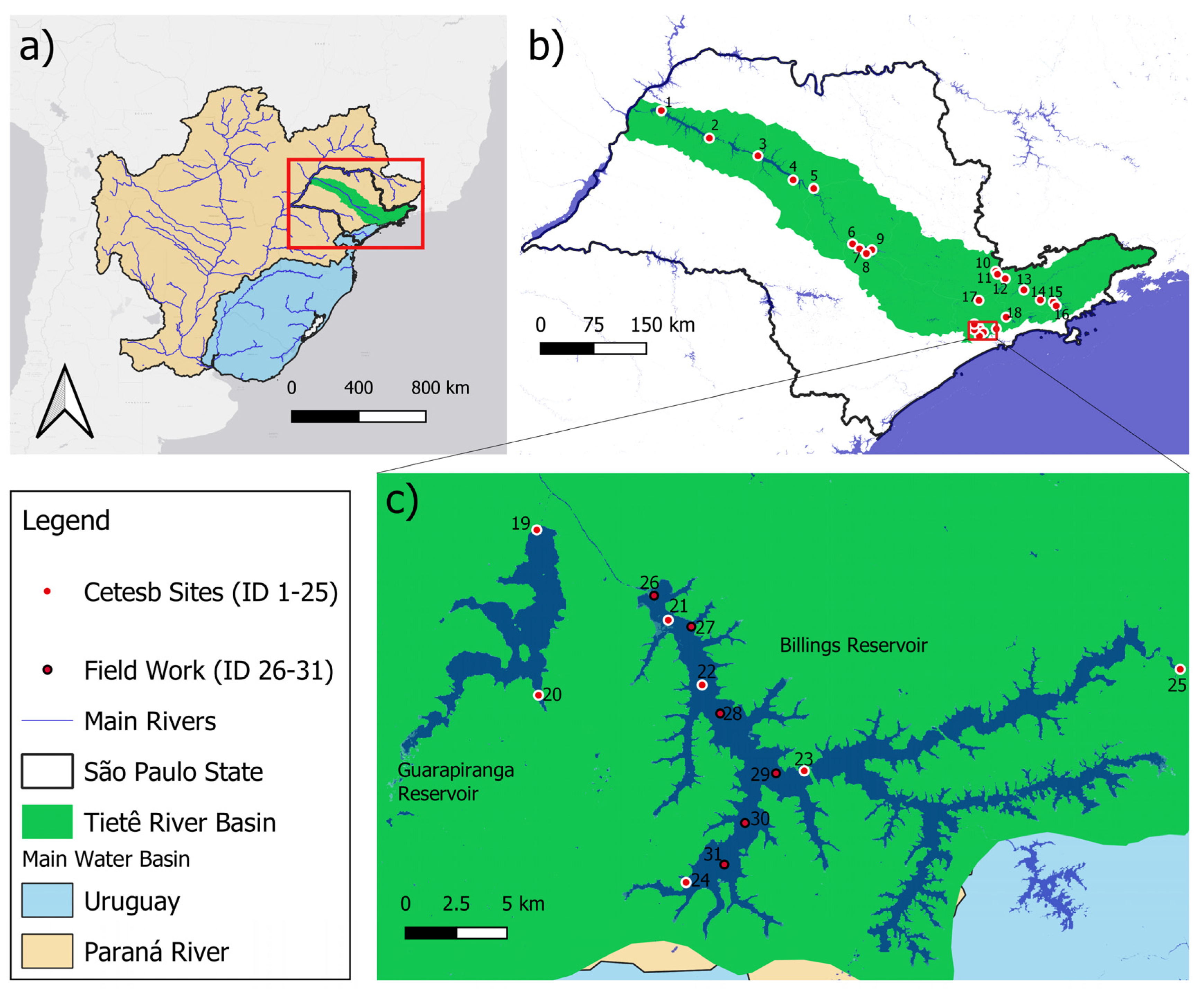
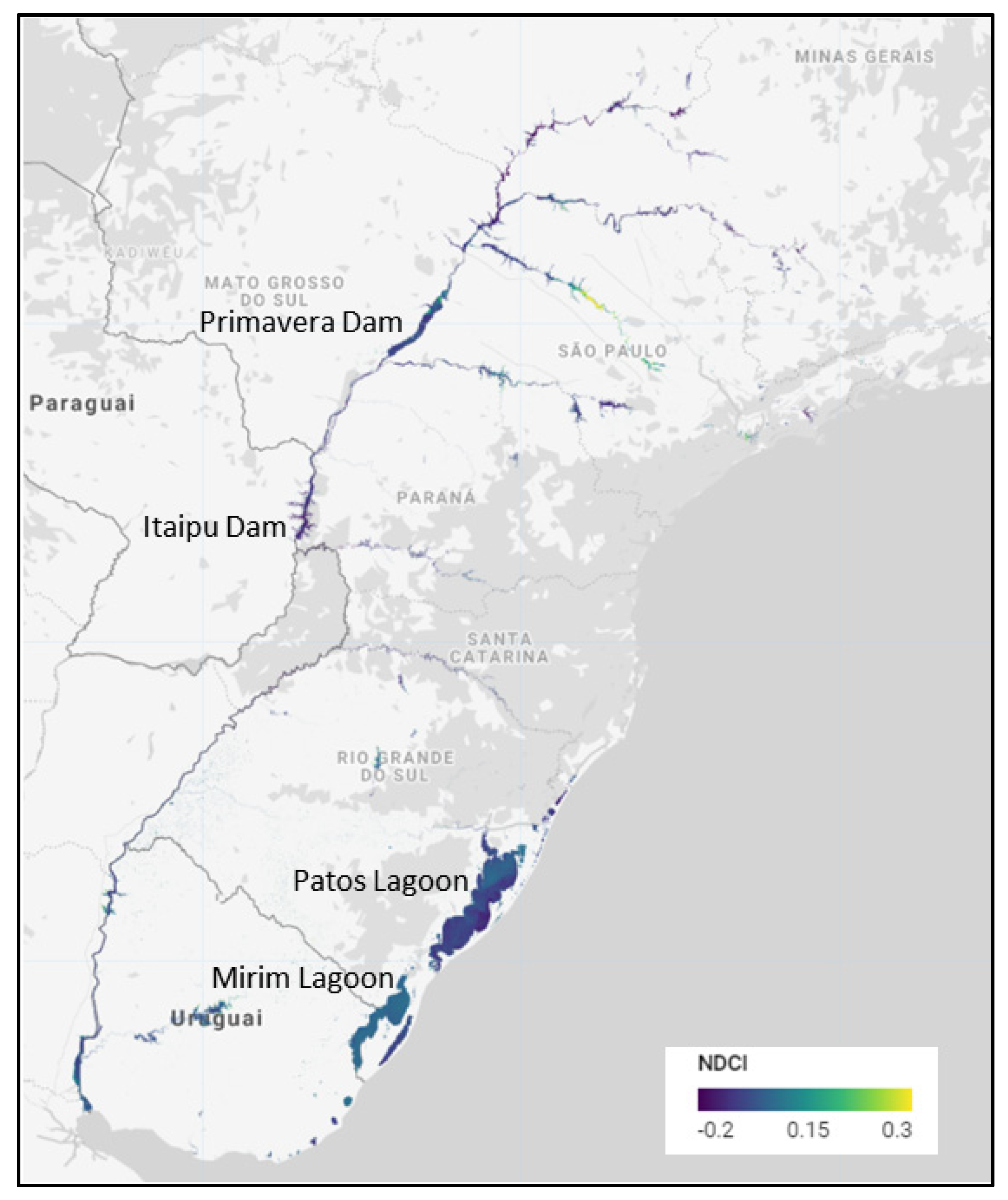
2.1. Tietê River Basin

The AB monitoring tools were first developed for selected reservoirs of the Tietê River Basin, located in the State of São Paulo (Figure 1), which is home to more than 40 million inhabitants and is responsible for more than 24% of the total water demand in Brazilian urban areas. A variety of reservoirs provides water for the urban areas within the State of São Paulo. The Cantareira system is the most important water supply for the São Paulo capital, while the Tietê Cascade System Reservoir (which comprises six reservoirs in its cascade system) with a downstream length of 1100 km provides water to fishery activities, navigation, hydroelectricity, industrial use, agriculture, and domestic demands for the interior of the State. However, the rapid urbanization and industrialization process has led to high nitrogen and phosphorus concentrations in surface waters and consequently degradation and eutrophication of the water quality [24]. For example, the Billings reservoir, located in the upstream Tietê basin, faces serious water pollution problems due to the increase in urban population without a concurrent increase in sewage or solid waste collection and treatment systems. As a result, high TSI levels were often observed throughout the past years [8] along the Tietê River expressed by Chl-a concentration ranging from 1 to over 500 µg/L, suitable for the proposed application because it covers a large variety of trophic levels, including AB conditions.

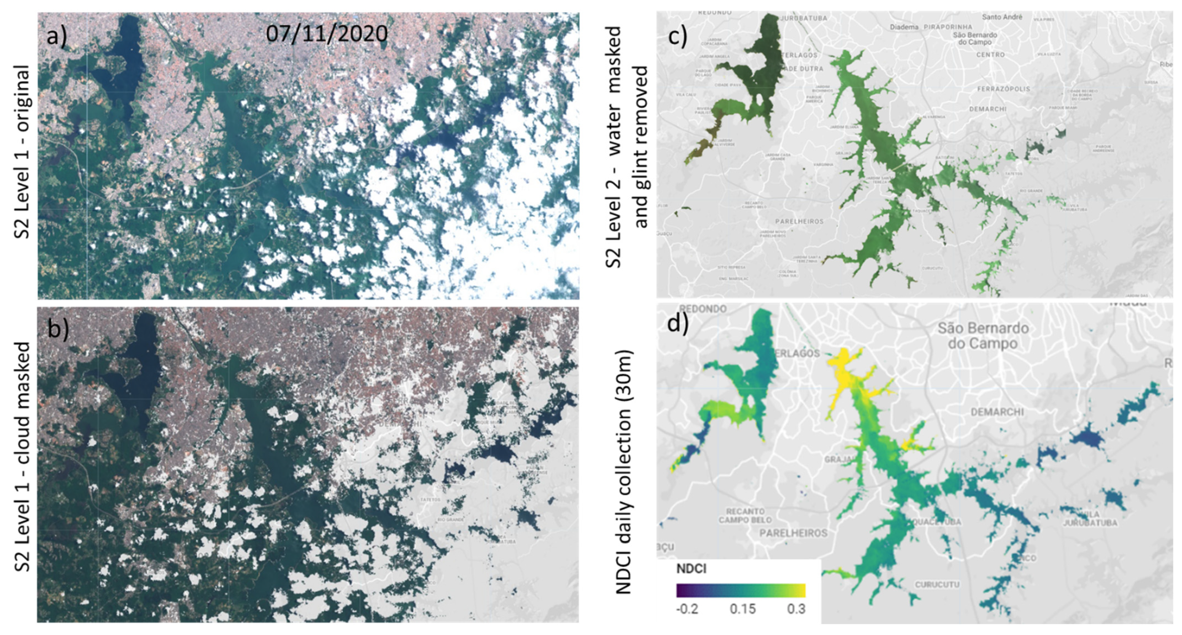
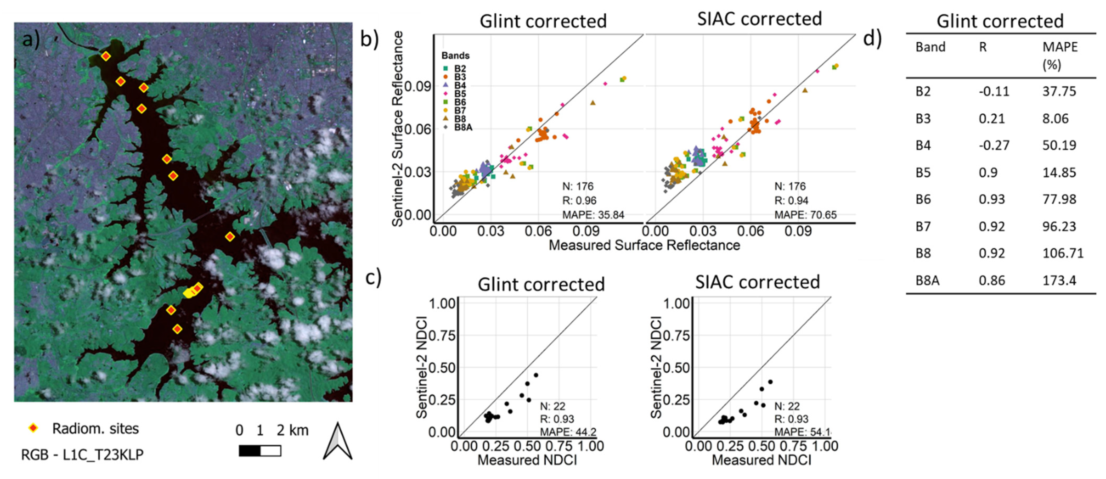
2.2. Sentinel-2 MSI Imagery Processing

The first step of the AB monitoring tool (Figure 2) is the atmospheric correction since water applications demand reliable surface reflectance measurements. To circumvent the lack of Sentinel 2 Level 2 (surface reflectance) for the entire time series (2015 onwards), the best option is to use the SIAC (Satellite Invariant Atmospheric Correction) implemented on GEE. The SIAC method uses coarse-resolution data derived from MODIS (Moderate Resolution Imaging Spectroradiometer) MCD43A3 datasets (at 500 m of spatial resolution) to describe surface anisotropy and CAMS (Copernicus Atmospheric Monitoring Service) to estimate atmospheric parameters. MODIS data is mapped to TOA (Top-of-Atmosphere) to be compared against data with coarser spatial resolution, and CAMS data is used to obtain atmospheric parameters solving an inversion problem. More detailed information about SIAC and its implementation in GEE can be obtained in Yin et al. [25] and in Song et al. [26].
After atmospheric correction, the sun glint effect was corrected by subtracting the B12 (2190 nm) from Bands 2–11 (Figure 2b). This method assumes that the remaining signal (after atmospheric correction) in the SWIR band is related to the air–water interface specular reflectance (sun and sky glint). The water signal in these wavelengths is assumed to be negligible due to the extremely high water absorption [27,28]. This method was previously used for glint correction in Brazilian waters with successful results [29,30,31,32]. In order to evaluate both atmospheric and sun-glint correction of a Sentinel-2 image, in situ radiometric data were collected in November 2020 in the Billings Reservoir. A detailed description of this evaluation can be found in Appendix A.
The next step is to mask out the pixels with clouds by applying the Sentinel-2: Cloud Probability product available on GEE (Figure 2c). This is a product created by using the Sentinel Hub’s cloud detector (s2cloudless python package), which provides automated cloud detection for Sentinel-2 imagery. Only pixels with a cloud probability lower than 10% were included in the following steps.
For the water mask, the Joint Research Centre (JRC) Water Mask product available on GEE was used [33] to include water masses that are permanent all year long to avoid adjacency effects and seasonally flooded wetlands (Figure 2d). After all the pre-processing steps were completed, NDCIsat was calculated (Figure 2e) as follows [9]:
NDCIsat = (SR705 – SR665)/(SR705 + SR665)
For Sentinel-2, the central wavelengths for Surface Reflectance at 705 nm (SR705) and at 665 nm (SR665) correspond to Band 5 (red edge) and Band 4 (red), respectively. The main limitation of using SIAC within GEE is that when the user wants to display the results on the map after SIAC’s correction, GEE reaches its maximum computing capacity. This limitation prevents the user from performing long time-series analysis of large water bodies. To overcome this issue, a new NDCIsat image collection has been created (resampled to 30 m) and uploaded into the GEE user’s asset to be used directly on the GEE platform (Figure 2f). By doing this, the user can perform spatial and temporal analysis of NDCIsat and derived products over large areas and long periods in a few seconds. Figure 2g,h refers to the calibration and validation of Chl-a and TSI algorithms, respectively, described as follows.

2.3. Chl-a In Situ Data

In situ Chlorophyll-a measurements were provided by the São Paulo State Environmental Company (CETESB), which monitors reservoirs bi-monthly at defined sample stations [23]. Considering the limited number of Chlorophyll-a in situ samples available on the same day as the satellite image acquisition, different time windows were tested to gather a larger number of samples (see Appendix B). After testing the algorithm’s output varying time windows from 0 to ±3 days, that with ±2 days has shown to be the best balance between the number of samples, accuracy, and precision for both Chl-a estimation and TSI classification. This time window has been frequently reported in the literature for the application of satellite images in lentic aquatic systems [34].
The two-days window matchups correspond to 130 samples of 25 stations (Figure 1 and Table 1) acquired from August 2015 and November 2020. Those samples are not evenly distributed amongst the in situ stations (IDs) since the frequency of Chl-a measurements varies among them—for example, Billings Reservoir’s stations ID21–25 are more likely to fall within the ±2 days window, having a larger number of samples throughout the study period. In addition, some fieldwork was conducted in the Billings Reservoir (in November 2020) during which six Chl-a concentration samples were incorporated to the calibration/validation dataset used to develop the Chl-a model (summing to a total of 136 pairs of Chl-a and NDCIsat samples, Table 1).

2.4. Calibration and Validation

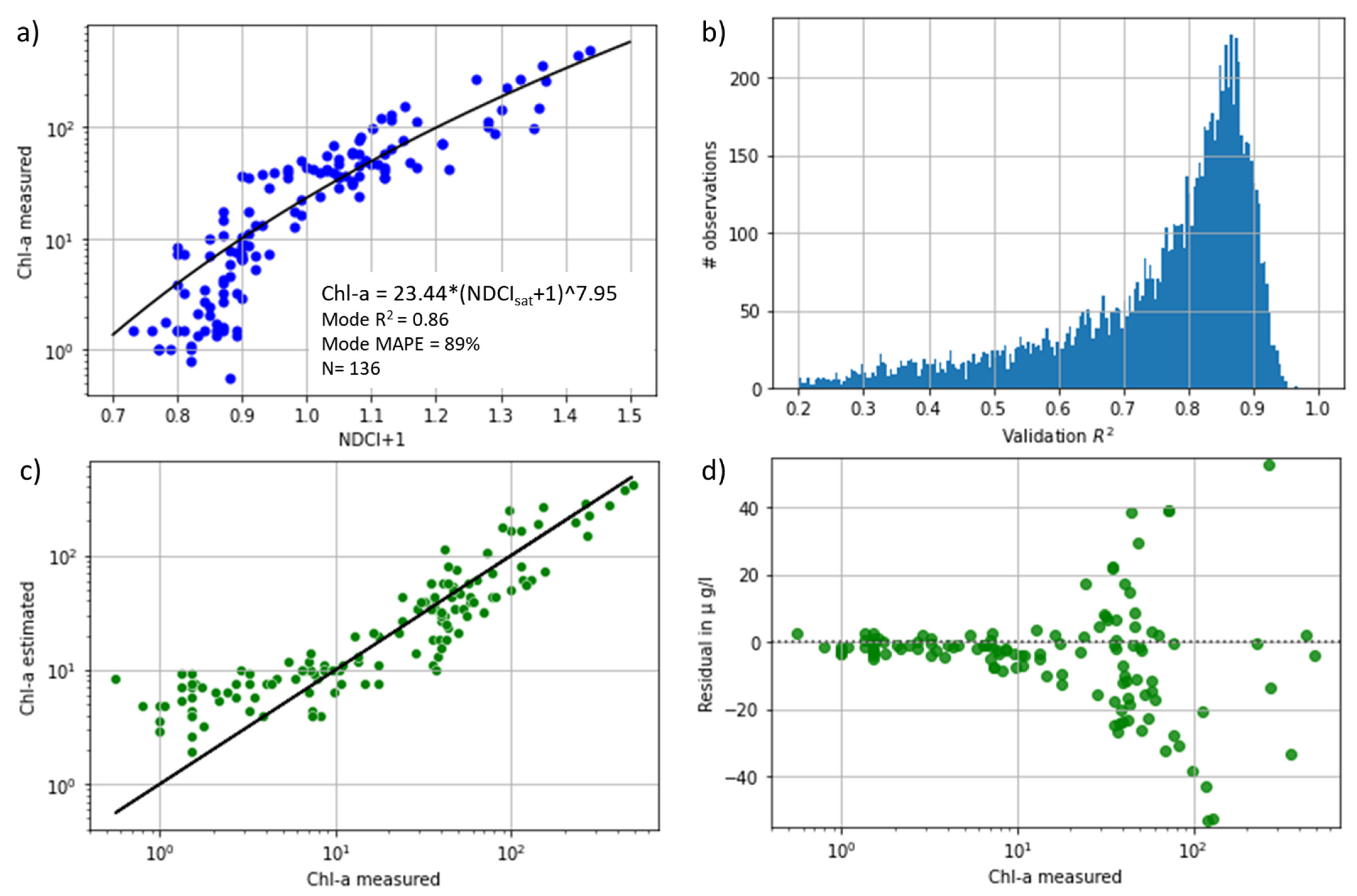
2.4.1. Algorithm for Chl-a

All the match-ups between in situ Chl-a data and NDCIsat (N = 136, for a ± 2 days’ time window) were used to calibrate the Chl-a algorithm by Monte Carlo (MC) cross validation technique, with 10,000 rounds [35]. At each run of Monte Carlo, 70% of the samples were applied for calibration and the remaining for validation (Figure 2g). After testing two non-linear fitting models (Polynomial 2nd order and power-law fitting curves), the power-law function was selected for the Chl-a modeling as the polynomial fitting showed a parabolic trend causing the estimated Chl-a to increase as NDCI decreased (for NDCI lower than −0.2). A total of 10,000 runs were used for Monte Carlo validation and two fitting statistics were computed: Coefficient of Determination, R2, and Mean Absolute Percentage Error, MAPE.
R 2 = 1   ( y i y ^ ) 2 ( y i y ¯ ) 2
MAPE = 100 n i = 1 n | y i y ^ y i |
where n is the number of predictions, y i is the observed value, y ^ is the predicted value, and y ¯ is the mean value of y i . The results for fitting statistics as well as the model parameters for the 10,000 runs were calculated considering the mode of each statistic.

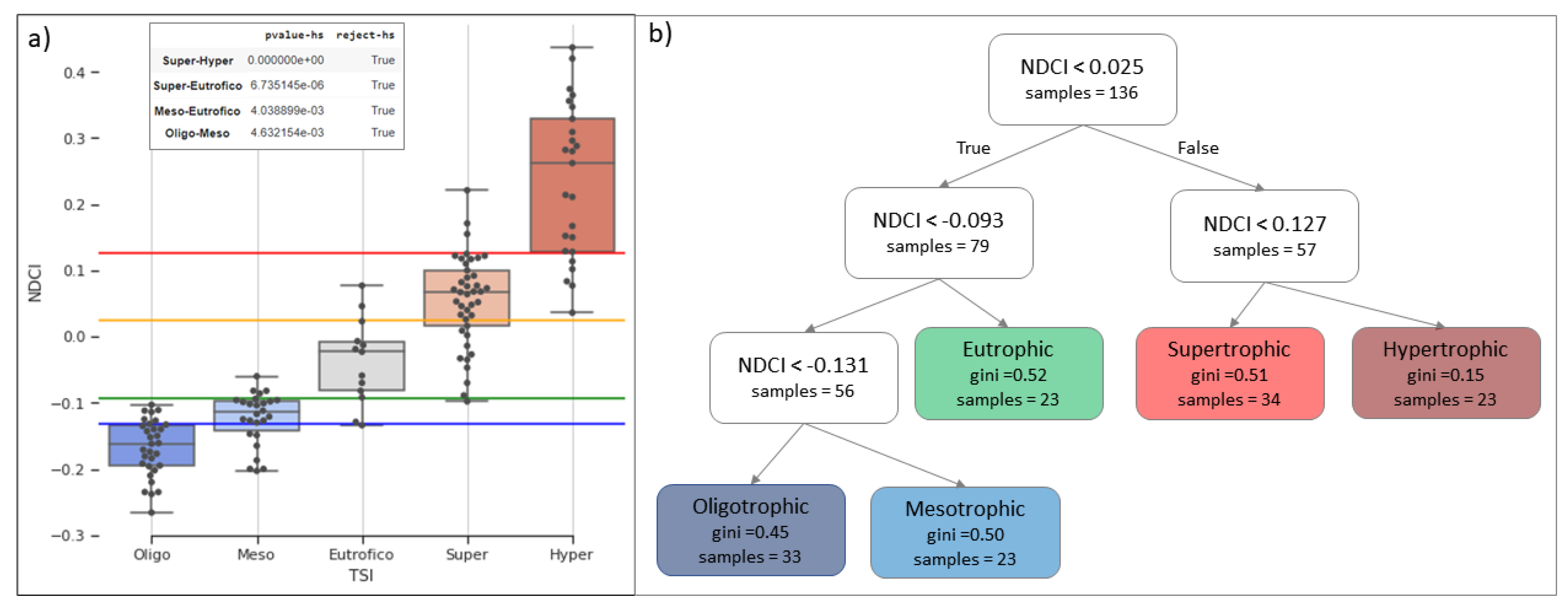
2.4.2. Decision Tree for TSI and Algae Bloom Classification

The Trophic State Index can be classified into six classes according to Chl-a concentration, ranging from Ultra-oligotrophic to Hyper-eutrophic (Table 2). For this study, all the 136 measured Chl-a samples were first categorized into measured TSI levels as ground truth following the thresholds in Table 2. The NDCIsat distribution for each TSI class was submitted to a paired T-Test (p value = 0.05) between the classes, where the null hypothesis is that there is no significant difference between the two classes being tested. The NDCIsat distributions between all classes were statistically different, except for Ultra-oligotrophic (not statistically different from Oligotrophic, p-value > 0.05) which was then reclassified into Oligotrophic. A decision tree based on MC technique was applied to determine the NDCIsat threshold that classifies into five TSI levels (Figure 2h). To detect the algae bloom (AB), the criterion was to consider either Super-eutrophic or Hyper-eutrophic levels (i.e., Chl-a > 30.55 µg/L) as algae bloom condition. The output is binary classification, where NDCIsat is categorized either as non-bloom (Oligo, Meso and Eutrophic levels) or AB condition (Super and Hypereutrophic levels).
For both TSI and AB detection, confusion matrices were used to evaluate the classification performances in terms of accuracy and f1-score. All the calibration and validation processing were conducted in Python 3.6.

2.5. GEE App

The Chl-a algorithm (Section 2.4.1) and TSI decision-tree (Section 2.4.2) were implemented in GEE in order to compute Chl-a, TSI, and AB maps from the stored NDCIsat collection (August 2015 to March 2021). To make these products easily accessible to end-users, a GEE App with interactive functions has been implemented. The user can select the Region of Interest (ROI), date range, and the type of analysis: either single image or temporal analysis. For single image analysis, the user can select an image from a day of the year to visualize RGB, NDCIsat, Chl-a, TSI, and/or AB images. For the temporal analysis, a couple of charts will pop-up when the user defines a geometry on the Map showing Chl-a temporal average and the relative TSI area. In addition, new map layers are added with mean, minimum, maximum maps for Chl-a, TSI, and AB data (Figure 2i).

3. Results

The intermediate outputs of an image processing workflow from Original S2 Level 1 to NDCI images are shown in Figure 3. The original image (Figure 3a) was first cloud masked (Figure 3b) and then submitted to atmospheric and glint correction followed by water mask application (Figure 3c). NDCIsat was calculated and exported to the NDCI-daily collection with a 30 m resolution (Figure 3d). The evaluation of the atmospheric correction method applied in this study is available in Appendix A.
After processing the entire Sentinel-2 imagery database for the Tietê River Basin on a daily basis and adding them into the GEE Asset with 30 m resolution, the NDCI daily collection of more than 1500 images from August 2015 to February 2021 summed up to 10 GB.

3.1. Chl-a Algorithm

As a result of Monte Carlo simulation, the validated power-law fitting curve (N = 30%) assembles the global power-law fitting curve (N = 136) rendering a robust predictive model (Figure 4a).
Chl-a = 23.44 × (NDCIsat +1) ^ 7.95
The final model presented a R2 of 0.86 and MAPE close to 90% (Figure 4a). The low accuracy indicated by MAPE value could be related to the fact that the proposed algorithm presented higher uncertainty for low Chl-a values (<5 µg/L). As Chl-a increases, the algorithm accurately estimates Chl-a for concentration between 10 and 70 µg/L, as observed in Figure 4c. On the other hand, the prediction’s errors increase significantly above 70 µg/L [Chl-a], according to the model’s residual values (Figure 4d). Overall, the algorithm performs satisfactorily well on estimating medium to high Chl-a (>10 µg/L), a concentration range where AB often occurs.

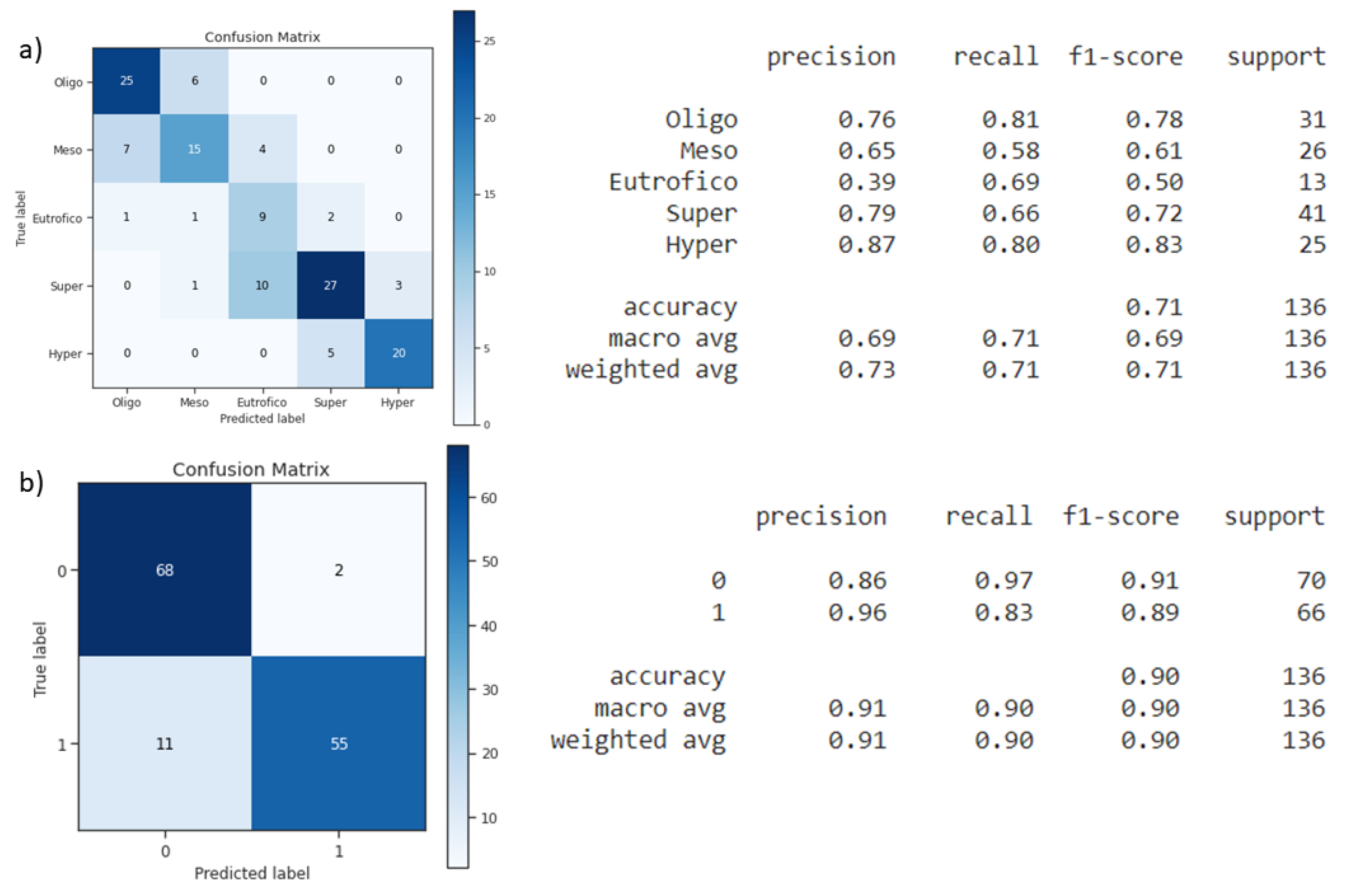
3.2. TSI Classification Tree

The paired T-test confirmed that the NDCIsat distribution is different among each TSI class (Figure 5a). The NDCIsat thresholds (nodes) were based on the decision tree defined after MC iteration (Figure 5b), as follows: <−0.131 (Oligo), <−0.093 (Meso), <0.025 (Eutrophic), and <0.127 (Super). The Gini index indicates high purity for Hypereutrophic class (n = 23). On the other hand, Gini increases for Meso (n = 23), Eutrophic (n = 23), and Super-eutrophic (n = 34) classes showing some overlap amongst them, as displayed in the boxplot.
The weighted overall f1-score, which accounts for both precision and recall, is 0.71 (Figure 6a). Oligo and Hypertrophic classes show a high f1-score (>0.78), indicating that the tree classification performs well on the extremes (very low and very high) of Chl-a concentration range. For the intermediate classes, however, the f1-score decreases to 0.72 for Super-eutrophic, 0.61 for Meso, and 0.50 for Eutrophic class. The Eutrophic class shows a low precision (0.39) due mostly to the underestimation of Super-eutrophic class, i.e., the tree decision classifies some Super-eutrophic samples (n = 10) as Eutrophic, and to the overestimation of Meso-eutrophic samples classified as Eutrophic class (n = 4). Overall, the classifier shows a satisfactory performance allowing the user to detect increasing levels of eutrophication.
For AB (Super and Hyper-eutrophic) vs. non-bloom (Oligo, Meso, and Eutrophic) classification, the overall f1-score is 0.90 (Figure 6b). Most of the errors are due to the misclassification of bloom (true label) as non-bloom (predicted label), which means the under-estimation of bloom condition of around 14%. On the other hand, for the pixels classified as bloom with 96% of precision, only two samples identified as bloom out of 57 were mistaken.

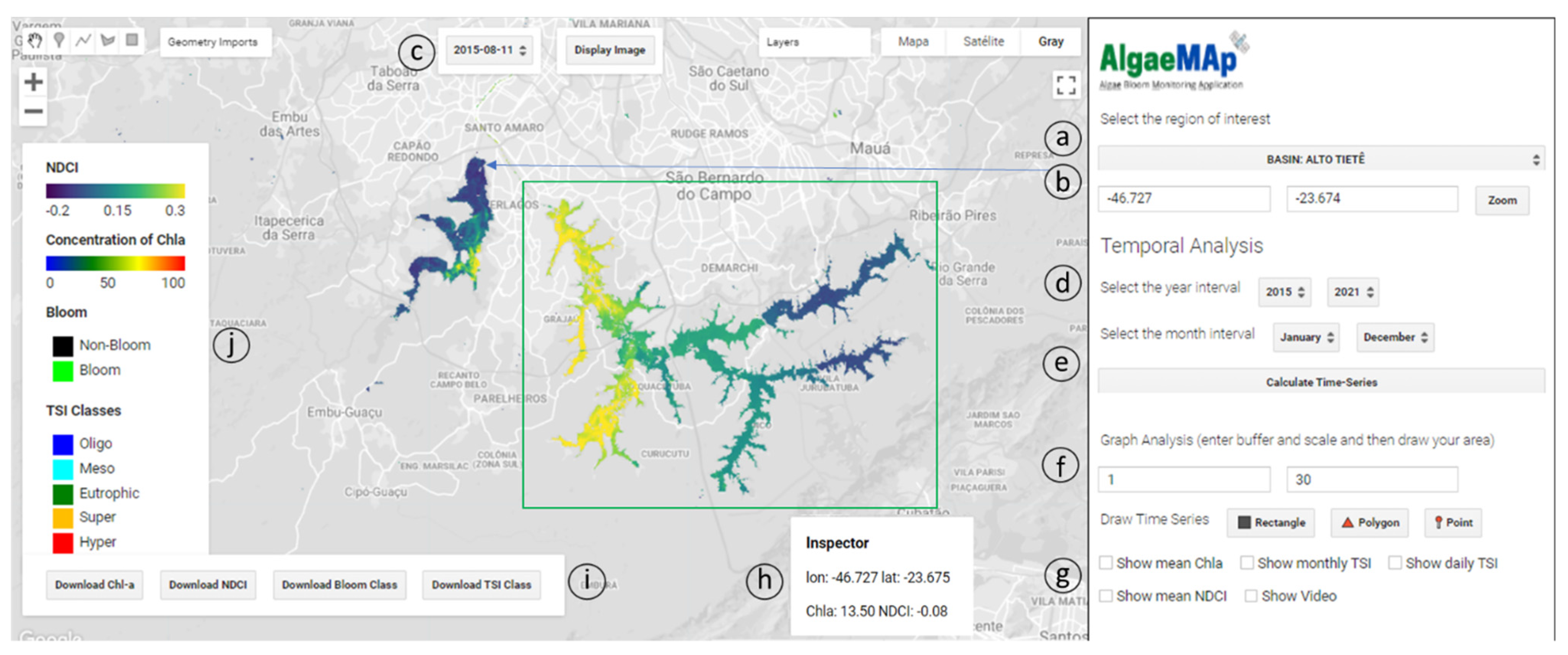
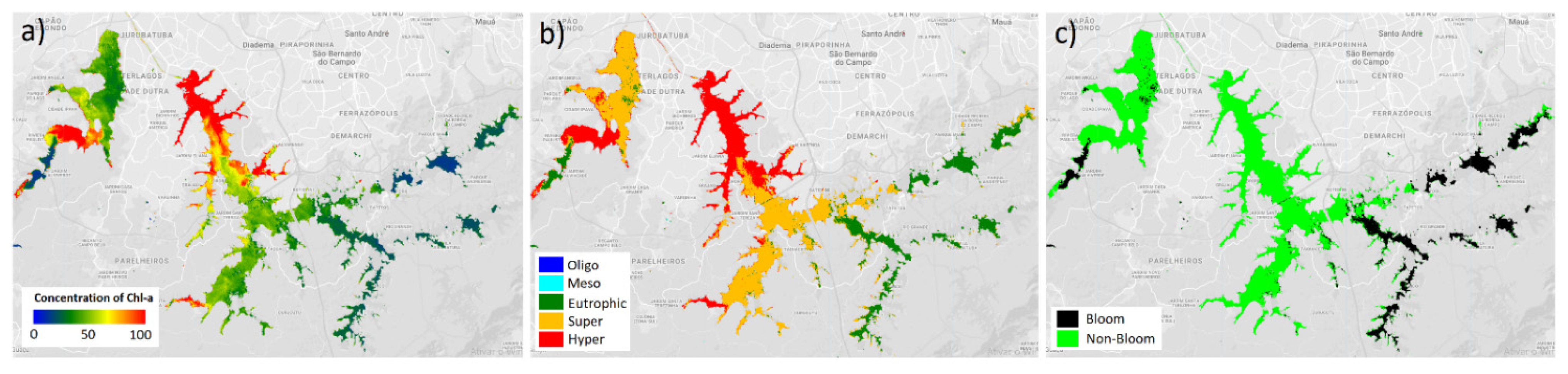
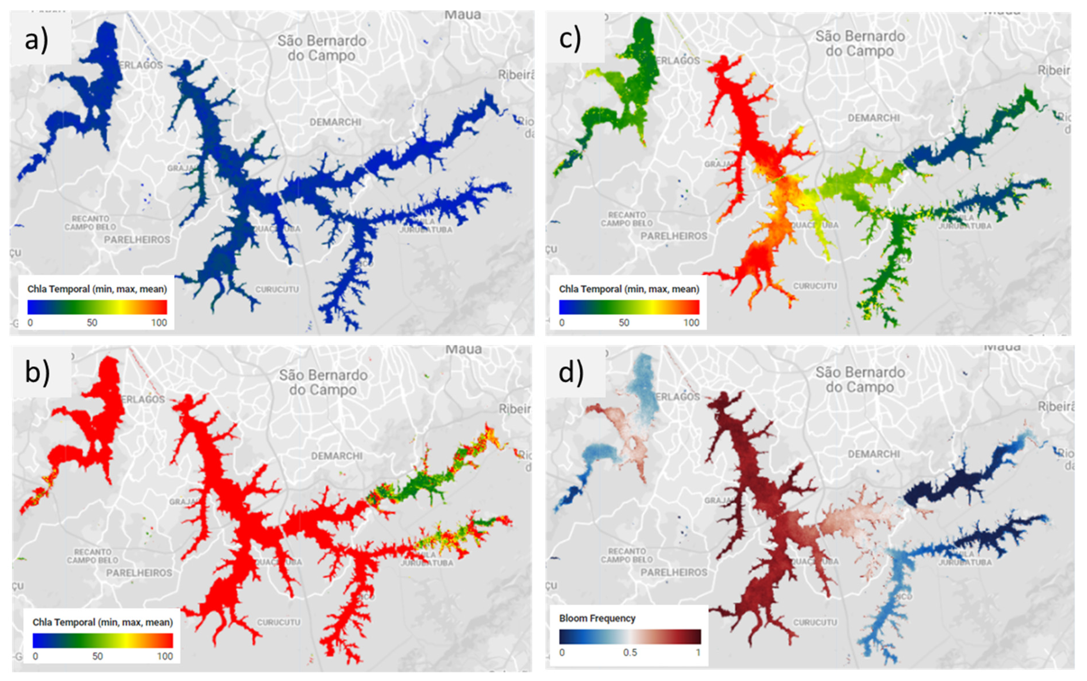
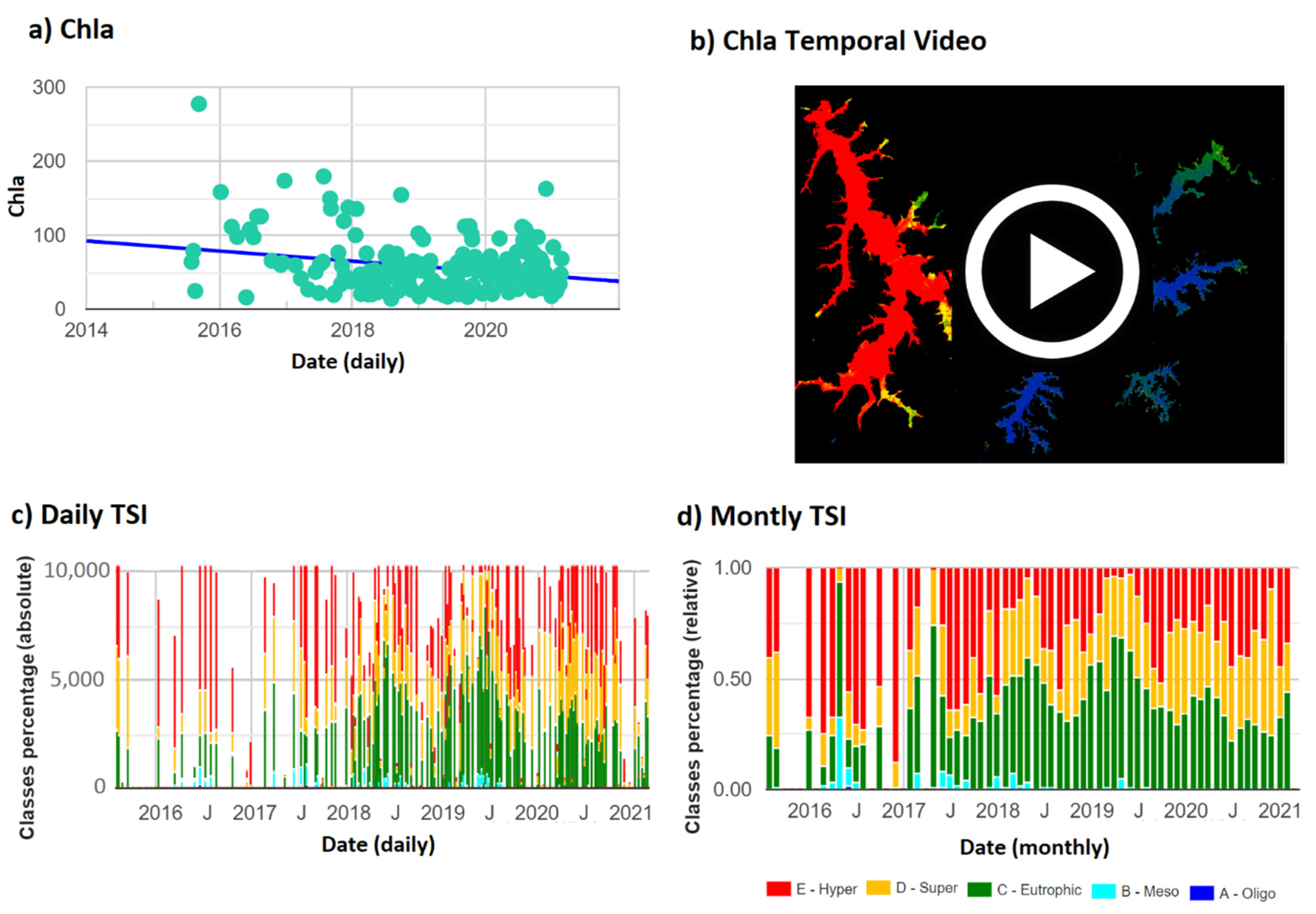
3.3. App Interface and Functionalities

Once the Chl-a and TSI algorithms had been calibrated and validated, they were implemented in GEE as an Earth Engine App (Figure 7), entitled Algae Bloom Monitoring Application (AlgaeMAp). Within the App, the user can pick a region of interest, display maps, create temporal charts, and visualize spatial stats, such as min, max, and mean values for each pixel given a date range.
A few examples extracted from the Tietê River Basin are shown to illustrate the App functionalities by taking the user’s perspective:
Single image analysis—After selecting a ROI (either basins or reservoirs), individual (or single) images can be displayed as RGB and/or derived products (Chl-a, TSI, bloom) by selecting the desired date (Figure 7c). After selecting the date, the user can click on the “Display Image” button (Figure 7c) to show the Chl-a, TSI, and Bloom images (Figure 8). For every date selected, the user can download the displayed layers (NDCIsat, Chl-a, TSI, and AB) as tiff files (Figure 7i). Additionally, the user can click on a given pixel to show the Chl-a, NDCIsat, and geographic location in the Inspector tool (Figure 7h).
Time-series spatial stats—After selecting the ROI, the user can also analyze time changes in variables such as Chl-a and NDCIsat (temporal mean, min, max) and Bloom Frequency (Figure 9). For that, the user must select the date range (year and month) and click on the ‘’Calculate Time-Series button’’ (Figure 7e). This method allows the user to choose a specific t interval and monthly range (to analyze seasonality). These statistical maps are added as new layers into the Map Panel and can be visualized and downloaded separately (Figure 9). Similar to the Single image analysis, clicking on a specific pixel on the map in the Time-series section will display the temporal variables in the Inspector (Figure 7h).
Time-series charts—After selecting the date range, the App can also be used to plot temporal information from an area of interest, which can be a rectangle, polygon, or point (Figure 7f). First, the user must choose one of these three available geometries and draw it on the map. Then the user must click on the desired information, which can be “Show mean Chl-a”, “Show mean NDCI”, “Show monthly TSI”, “Show daily TSI”, and “Show Video”. For the “Show mean Chl-a” and “Show mean NDCI” buttons, the App displays temporal variation of spatial mean Chl-a and NDCI (if the geometry is a rectangle or a polygon). When the user selects a point, the Chl-a and NDCIsat temporal information becomes specific to an individual pixel. As a result, the Chl-a and NDCIsat time series can be analyzed for a given geographic coordinate of interest (decimal longitude and latitude, WGS 84), which is often the case when you have in situ data from a field campaign. For example, Figure 10a shows Chl-a time-series for one of the CETESB’s monitoring sites indicated by the coordinates in Figure 7.
Furthermore, it is possible to identify, within the chart, every date with an image, which can be then displayed (Figure 8c). For TSI, there are two options to visualize the information: relative TSI area aggregated by month (“Show monthly TSI”) or absolute daily TSI area (“Show daily TSI”). Monthly aggregation gives a more general TSI condition with less gaps on the water body over space and time, being more appropriate for long-term and regular monitoring. Alternatively, for a more specific evaluation of TSI, the user can select aggregation by day which shows the absolute number of pixels for a given eutrophication class. Figure 10c,d shows the TSI temporal trend aggregated by day and month within the rectangle presented in Figure 7 (covering the entire Billings reservoir). Additionally, the user can visualize a video of Chl-a maps over time when selecting “Show Video” (Figure 10b).

4. Discussion

The monitoring of Chl-a concentration in inland waters using remote sensing data has been improved in the last years due to the new generation of earth observation sensors [10]. A successful example is the MSI sensor aboard Sentinel-2A-B. This sensor covers the lack of spectral (13 bands), spatial (10–20 m), and temporal (5 days) resolutions required for inland water bodies monitoring [10,13,36,37]. Moreover, the MSI sensor’s spectral resolution allows for Chl-a concentration in those waters to be detected more accurately than in other sensors such as Landsat-8 [38]. This accuracy is likely due to there being more bands in the near-infrared region (705, 740 nm), which allows the detection of the spectral features associated to phytoplankton blooms (e.g., high Surface Reflectance signal at 705 nm). Therefore, these spectral features could be enhanced using indexes such as the NDCI [9]. NDCI is related to Chl-a as it is the normalized difference between the red-edge band (705 nm) and the red band (660 nm) [39]. As Chl-a concentration increases, the signal at 705 nm will increase (reflectance peak), and the signal at 660 nm will decrease due to the high Chl-a absorption at this band [9]. NDCI and band ratios between red-edge and the red band were widely evaluated in literature and presented successful results [9,36,40,41,42,43,44].
In this study, the use of NDCIsat for estimating Chl-a concentration in the Tietê River Basin confirms its applicability for algae blooms monitoring. It was possible to develop a robust power-law function to predict Chl-a based on NDCIsat values obtained from the Sentinel-2 images. The results based on our validation procedure using Monte Carlo simulation demonstrated that the model had good performance for Chl-a retrieval (mode of R2 = 0.86). Further, the NDCIsat separated the trophic state (global accuracy of 0.70) and the bloom occurrence (global accuracy of 0.90). In a previous NDCIsat application on MERIS bands, Mishra [9] used a quadratic function to estimate Chl-a from the NDCIsat (Chl-a < 30 μgL−1), with RMSE of 1.43 μgL−1. In a eutrophic reservoir in Tietê River Basin (Barra Bonita), Watanabe et al. [43] obtained an R2 of 0.80 and a Mean Absolute Error (MAPE) of 39.44% for an NDCI algorithm, using in situ radiometric measurements. In a more global application for a wider range of Chl-a concentrations (0–1000 μgL−1), Pahlevan et al. [37] reported that NDCI obtained from in situ radiometric data estimated Chl-a with errors of approximately 49%. The NDCI was compared with other algorithms and outperformed almost all, apart from a machine-learning algorithm. Using Sentinel-2 imagery, Watanabe et al. [45] observed that NDCI performed better than other algorithms (2-band, 3-band, and slope) for Chl-a retrieval in the Tietê cascade system (Chl-a between ~0 to up to 800 μgL−1), with MAPE values of 48%. The use of NDCI for Chl-a estimates in eutrophic environments (~40 to up to 225 μgL−1) was also demonstrated by Tavares et al. [46] in two Brazilian Lagoons (RMSE = 25.96 μgL−1). Additionally, NDCI has been used for algal bloom monitoring in locations with the absence of in situ data due to the COVID-19 lockdown [12,47], and also to provide near-real-time bloom alerts to environmental and governmental agencies [10,11].
The performance of NDCIsat algorithm for Chl-a retrieval using satellite data is dependent on the atmospheric correction. In Google Earth Engine, bottom of atmosphere (BOA) data was only available using the Sen2Cor method and only after 2019 for the South America region. The Sen2Cor method that generates the BOA data for MSI imagery in GEE also has uncertainties for water applications, as it is designed for land applications [48]. Therefore, atmosphere correction methods suitable for inland water application need evaluation to increase their accuracy over water bodies. The SIAC method evaluated in this study presented a satisfactory performance for Surface Reflectance retrieval (Pearson R = 0.96, MAPE = 48%) when all bands were compared and, specifically, for bands used in the NDCIsat calculation (MAPE = 27.23% and 8.92% for bands 4 and 5, respectively). Similar to other AC methods, SIAC applies the well-known 6SV RT model, a long-term MODIS product, as well as fast processing in the GEE platform. Moreover, the auxiliary products have been tested for atmospheric correction of medium spatial resolution [49,50,51], and the results are promising in terms of quality and reproducibility. In fact, the satisfactory agreement between in situ surface reflectance and satellite reflectance corroborates the use of SIAC for water quality applications, particularly for NDCIsat calculation. The advantage is that SIAC has been implemented into GEE allowing atmospheric correction via cloud computing services, which is extremely fast when compared to traditional personal computing methods.
Furthermore, we observed that glint correction reduced Surface Reflectance data errors (a reduction by, approximately, 30%). The application of glint correction using the SWIR band of Sentinel-2 was also demonstrated by other studies in Brazilian Inland waters [29,31,35]. The comparison between in situ calculated NDCI and NDCIsat also presented likely results (Pearson R = 0.94, MAPE = 47.4%). The higher MAPE values for NDCI could be attributed to uncertain propagation in band-ratio algorithms [52], and a slight offset between in situ measured and NDCIsat. However, as the algorithms were developed using NDCIsat on a wide temporal scale, this difference should not impact the final algorithm. The time delay used in this study was set at ±2 days, which could be a source of uncertainty if a bloom occurs between these two measurements [53,54]. However, other studies pointed out that if the data was carefully checked, the time delay could be extended up to three days [29,35,45,55].
For the TSI, previous studies [29,55] usually estimate trophic levels after deriving Chl-a concentration from satellite imagery, which often propagates the Chl-a algorithm’s uncertainties. Alternatively, we propose the use of NDCIsat, which is independent of any predictive Chl-a algorithm, to derive TSI levels. The proposed decision tree separates extreme classes well, such as Oligotrophic and Hypereutrophic, but some misclassifications were observed within the intermediate levels. It is important to note that both Chl-a and TSI algorithms are results of the first attempt at a regional approach. The plan is to improve these algorithms, having NDCIsat as the predictive index so it can be extended to other relevant regions in Latin America (Figure 11).
Overall, the AlgaeMAp application system has shown to be useful to provide remote sensing water quality algorithms to end-users. The App is easy to use and offers valuable information about the current and historical Chl-a, TSI, and bloom state of a given water body. Different programs have been developing platforms to monitor reservoir Chl-a and trophic state using remote sensing [56,57,58]. The CyanoLakes company, for example, monitors current and historical Chl-a in reservoirs using the Ocean and Land Colour Instrument (OLCI) on Sentinel-3 (with 300 m spatial resolution) and provides the information in a web platform [58]. Similarly, the company EOMap also provides web portals where the user can extract spatial and temporal data of Chl-a, suspended matter, Chl-a, harmful algae bloom, and trophic state classification [56]. In addition to private companies, public agencies are also realizing the great benefit of providing water quality parameters in web platforms. The Brazilian National Water Agency (in Portuguese ANA) has been developing a remote sensing web platform called HidroSat, which provides Chl-a and turbidity information using MODIS TERRA e AQUA [59]. However, the platform provides the historical information in a graph for just one fixed point, a method that prevents spatial analysis. In the same way, the United States Environmental Protection Agency (EPA) has been developing an App that will inform cyanobacteria algal blooms on a national scale throughout the USA using Sentinel 3 information [57].
To the extent of the authors’ knowledge, our developed AlgaeMAp is the first online platform built within the GEE platform to offer high spatial resolution of water quality parameters. As a result, the App benefits from the huge processing capability of the GEE platform that allows any user with internet access to easily extract detailed spatial (30 m) and long temporal Chl-a and TSI information (from August 2015 and with images every five days) over the most important reservoirs in São Paulo. AlgaeMAp uses the GEE platform to access Sentinel 2 images which are uploaded approximately one day after the satellite acquisition date, allowing the App to serve as an alarm system as well. Considering that the São Paulo State Environmental Quality Company currently relies on in situ data to monitor reservoirs in the most important economic region in Brazil, the App satellite information might be a huge advance in water governance if incorporated by water agencies. The AlgaeMAp aims to connect space technology to water decision end-users to improve water management in Latin America.

5. Conclusions

In this article, we demonstrate the development of an algae bloom monitoring system that uses cloud computing (GEE) to process all Sentinel-2 imagery, generate the NDCIsat collection, and provide quick access to the Chl-a and TSI (Trophic State Index) levels for any water body within the study area (Tietê River Basin, Figure 1). More importantly, all this information has been implemented into an Earth Engine App that allows personalized evaluation of a given water mass that can either be chosen from a list or drawn by the user on the map panel. The AlgaeMAp is currently under development and a demonstration version can be accessed from GEE App gallery Available online: https://felipellobo.users.earthengine.app/view/algaemapv10 (accessed on 8 July 2021). The user is able to define date range, ROI (Region of Interest), time-series charts (either NDCI or Chl-a) and TSI area charts (% class area), and save these plots as texts or image formats.
For the project’s following activities, we plan to extend the NDCIsat collection to other important South America regions, such as Uruguay, Argentina, and north-eastern Brazil. However, this extension depends on in situ data for algorithm validation, which could be accomplished with more in situ chlorophyll data provided by the users and collaborators. Finally, this project represents the state-of-art Application of Remote Sensing and Cloud Computing to provide algae bloom alerts in the Latin America regions, helping governments, institutions, and decision-makers to take quick actions to protect and mitigate environmental impacts derived from algae bloom events.

Author Contributions

Conceptualization, F.d.L.L., C.C.F.B. and E.M.L.d.M.N.; methodology and application, F.d.L.L. and G.W.N.; field data validation, D.A.M. and C.C.F.B.; writing—original draft preparation, F.d.L.L., G.W.N. and D.A.M.; writing—review and editing, L.A.S.d.C. and V.S.M.; project administration, F.d.L.L. All authors have read and agreed to the published version of the manuscript.

Funding

This study was financed in part by the Coordenação de Aperfeiçoamento de Pessoal de Nível Superior-Brasil (CAPES)-Finance Code 001, and by the Remote Sensing Program, Graduate Division, National Institute for Space Research (INPE).

Institutional Review Board Statement

Not applicable.

Informed Consent Statement

Not applicable.

Data Availability Statement

Chloropyll-a data are freely available in the INFOAGUAS CETESB website. In situ reflectance data are available from the authors upon reasonable request. Sentinel-2 data are freely available in Google Earth Engine platform.

Acknowledgments

The authors would like to thank CETESB for providing water quality parameters. Authors would also like to than Juan Torres-Batllo (EO Data Science) for crucial help in Google Earth Engine App implementation. Authors are in debt to Felipe Nincao, Rejane Paulino, and Rogério Flores Júnior (INPE’s Postgraduate Course) for help with in situ measurements in Billings Reservoir.

Conflicts of Interest

The authors declare no conflict of interest.

Appendix A

For an evaluation of a Sentinel-2 images after atmospheric and sun glint correction, radiometric data was collected in the Billings Reservoir (November 2020). Three intercalibrated TriOS-RAMES (Hyperspectral Radiance and Irradiance Sensors) spectroradiometers, operating in the 350–950 nm spectral range, were used to collect radiometric data in 22 sample sites (Figure A1a, Chl-a concentration was only determined for six of these sample sites). At each site, the instruments measured, simultaneously, the downwelling irradiance above the water surface, Water-Leaving Radiance, and Sky Radiance to derive Surface Reflectance-SR (full radiometric processing described in [30]). Then SR values were used to simulate MSI/Sentinel-2 spectral bands using their Spectral Response Function [60].
SR ( λ j ) = i = 1 n SR ( λ i )   ×   SRF ( λ i )   i = 1 n SR ( λ i )
where SR ( λ j ) is the simulated band at central wavelength j, SRF (λ) is the spectral response function for each wavelength i, and SR ( λ i ) is the measurement for each wavelength i. The simulated bands were used to calculate NDCI (Equation (1)), named NDCIin situ, which were compared to the NDCIsat derived from Sentinel-2/MSI. In total, 22 radiometric samples were used to evaluate the Sentinel-2 processing of atmospheric correction, glint correction and NDCI of one image acquired on 7 November 2020 (Tile: T23KLP).
The evaluation of the SIAC’s surface reflectance output using in situ surface reflectance as ground truth (Figure A1) shows a high correlation between them (N = 176 considering all bands, R = 0.94, MAPE = 70.65%). Particularly, for Bands 4 and 5, used in NDCI calculation, MAPE was 50.19 and 14.85, respectively. The Pearson’s correlation and MAPE slightly improved after sun-glint correction of Sentinel 2 Surface Reflectance (SR) for this image (All bands, Pearson R = 0.96, MAPE = 45.09).
When in situ measured NDCI (NDCIin situ) is plotted against Sentinel-2 derived NDCI (NDCIsat), a high positive correlation is observed (R = 0.93. N = 22). NDCIsat consistently shows lower values, which is expected, because NDCIsat integrates a larger area (30 m × 30 m) than those measured by in situ radiometers.
Figure A1. (a) Location of the 22 radiometric samples acquired on 7 November 2020 in the Billings Reservoir; (b) Scatter plot between measured and satellite surface reflectance after atmospheric correction (SIAC) and glint correction considering B2 (490 nm), B3 (550 nm), B4 (665 nm), B5 (705 nm), B6 (740 nm), B7 (783 nm), B8 (842 nm), and B8A (865 nm), statistics (Pearson’s R and MAPE) for all bands together; and (c) Scatter plot between NDCIin situ and NDCIsat, statistics for 22 radiometric measurements. (d) Pearson’s R and MAPE for each band after SIAC and glint corrections (n = 22).
Remotesensing 13 02874 g0a1

Appendix B

To define a predictive model with the best balance between the number of samples, accuracy, as well as precision for both Chl-a estimation and TSI classification, several tests were taken by varying time windows from 0 to ±3 days. According to Table A1, the algorithm’s outputs with ±2 days has shown to be more appropriated for this application because it comprises a wide Chl-a interval, large number of samples (n = 136), and yet, high determination coefficient value (R2 = 0.86).
Table A1. Performance of power-law algorithm by varying the time window between satellite and in situ samples from 0 to ± 3 days. a and b refer to the algorithm’s parameters (Chl-a = a ∗ (NDCIsat +1) ^ b). The model chosen for this research is ± 2 days indicated with *.
Days (+ −)# of SamplesChl-a Range (µg/L)R2MAPEab
0270.56–87.60.650.2529.814.54
1910.56–486.10.860.5719.238.68
2 *1360.56–486.10.860.8923.447.95
31750.56–486.10.811.0024.497.48
For the TSI tree decision and AB classification, similar conclusions can be withdrawn. Overall accuracy for TSI classification when using a ± 2 days window is approximately the same as using ±1 day window but with 50% more samples (Table A2). For AB classification, overall accuracy is similar for all tested windows (>0.89). When using only samples taken on the same day (0 day), the paired T-tested amongst the classes did not reject the null hypothesis which is that there is no significant difference between them preventing procession with the tree decision testing.
Table A2. Accuracy performance of Trophic State Index (TSI) and Algae Bloom (AB) classification by varying the time window between satellite and in situ samples from 0 to ± 3 days. Paired T-test between classes rejects the null hypothesis (H0) when there is a statistical difference between them (p-value < 0.05). Nodes correspond to NDCI thresholds depicted in Figure 6. The model chosen for this research is ± 2 days indicated with *.
TSI AB
Days (+ −)# of SamplesChl-a Range (µg/L)T-Test
(reject H0)
AccuracyNode1-MesoNode2-EutroNode3-SuperNode4-HyperAccuracy
0270.56–87.6FALSE
1910.56–486.1TRUE0.714−0.150−0.0600.0250.1240.89
2 *1360.56–486.1TRUE0.705−0.131−0.0930.0250.1270.9
31750.56–486.1TRUE0.640−0.131−0.0990.0250.1270.89

References

  1. Branche, E. The multipurpose water uses of hydropower reservoir: The SHARE concept. C. R. Phys. 2017, 18, 469–478. [Google Scholar] [CrossRef]
  2. Teurlincx, S.; Kuiper, J.J.; Hoevenaar, E.C.M.; Lurling, M.; Brederveld, R.J.; Veraart, A.J.; Janssen, A.B.G.; Mooij, W.M.; de Senerpont Domis, L.N. Towards restoring urban waters: Understanding the main pressures. Curr. Opin. Environ. Sustain. 2019, 36, 49–58. [Google Scholar] [CrossRef]
  3. Kunz, M.J.; Wüest, A.; Wehrli, B.; Landert, J.; Senn, D.B. Impact of a large tropical reservoir on riverine transport of sediment, carbon, and nutrients to downstream wetlands. Water Resour. Res. 2011, 47. [Google Scholar] [CrossRef] [Green Version]
  4. Ho, J.C.; Michalak, A.M.; Pahlevan, N. Widespread global increase in intense lake phytoplankton blooms since the 1980s. Nature 2019, 574, 667–670. [Google Scholar] [CrossRef]
  5. Sanseverino, I.; Conduto, D.; Pozzoli, L.; Dobricic, S.; Lettieri, T. Algal Bloom and Its Economic Impact; Joint Research Center, European Comission (JRC), Institute for Environment and Sustainability: Ispra, Italy, 2016. [Google Scholar]
  6. Hamada, N.; Thorp, J.H.; Rogers, D.C. (Eds.) Thorp and Covich’s Freshwater Invertebrates; Academic Press: Cambridge, MA, USA, 2019; p. ii. ISBN 978-0-12-804223-6. [Google Scholar]
  7. Istvánovics, V. Eutrophication of Lakes and Reservoirs. In Encyclopedia of Inland Waters; Elsevier: Amsterdam, The Netherlands, 2009; pp. 157–165. ISBN 9780123706263. [Google Scholar]
  8. Watanabe, F.; Alcântara, E.; Rodrigues, T.; Rotta, L.; Bernardo, N.; Imai, N.; Sayuri, F.; Watanabe, Y. Remote Sensing of the Chlorophyll-a Based on OLI/Landsat-8 and MSI/Sentinel-2A (Barra Bonita reservoir, Brazil). Acad. Bras. Cienc Annals Braz. Acad. Sci. 2017, 1–14. [Google Scholar] [CrossRef] [Green Version]
  9. Mishra, S.; Mishra, D.R. Normalized difference chlorophyll index: A novel model for remote estimation of chlorophyll-a concentration in turbid productive waters. Remote Sens. Environ. 2012, 117, 394–406. [Google Scholar] [CrossRef]
  10. Caballero, I.; Fernández, R.; Escalante, O.M.; Mamán, L.; Navarro, G. New capabilities of Sentinel-2A/B satellites combined with in situ data for monitoring small harmful algal blooms in complex coastal waters. Sci. Rep. 2020, 10, 8743. [Google Scholar] [CrossRef] [PubMed]
  11. Aubriot, L.; Zabaleta, B.; Bordet, F.; Sienra, D.; Risso, J.; Achkar, M.; Somma, A. Assessing the origin of a massive cyanobacterial bloom in the Río de la Plata (2019): Towards an early warning system. Water Res. 2020, 181, 115944. [Google Scholar] [CrossRef] [PubMed]
  12. Rodríguez-Benito, C.V.; Navarro, G.; Caballero, I. Using Copernicus Sentinel-2 and Sentinel-3 data to monitor harmful algal blooms in Southern Chile during the COVID-19 lockdown. Mar. Pollut. Bull. 2020, 161, 111722. [Google Scholar] [CrossRef]
  13. Arabi, B.; Salama, M.S.; Pitarch, J.; Verhoef, W. Integration of in-situ and multi-sensor satellite observations for long-term water quality monitoring in coastal areas. Remote Sens. Environ. 2020, 239, 111632. [Google Scholar] [CrossRef]
  14. Bonansea, M.; Bazán, R.; Germán, A.; Ferral, A.; Beltramone, G.; Cossavella, A.; Pinotti, L. Assessing land use and land cover change in Los Molinos reservoir watershed and the effect on the reservoir water quality. J. S. Am. Earth Sci. 2021, 108. [Google Scholar] [CrossRef]
  15. Gorelick, N.; Hancher, M.; Dixon, M.; Ilyushchenko, S.; Thau, D.; Moore, R. Google Earth Engine: Planetary-scale geospatial analysis for everyone. Remote Sens. Environ. 2017, 202, 18–27. [Google Scholar] [CrossRef]
  16. Xiong, J.; Thenkabail, P.S.; Gumma, M.K.; Teluguntla, P.; Poehnelt, J.; Congalton, R.G.; Yadav, K.; Thau, D. Automated cropland mapping of continental Africa using Google Earth Engine cloud computing. ISPRS J. Photogramm. Remote Sens. 2017, 126, 225–244. [Google Scholar] [CrossRef] [Green Version]
  17. Hird, J.N.; DeLancey, E.R.; McDermid, G.J.; Kariyeva, J. Google Earth Engine, Open-Access Satellite Data, and Machine Learning in Support of Large-Area Probabilistic Wetland Mapping. Remote Sens. 2017, 9, 1315. [Google Scholar] [CrossRef] [Green Version]
  18. Jia, T.; Zhang, X.; Dong, R. Long-Term Spatial and Temporal Monitoring of Cyanobacteria Blooms Using MODIS on Google Earth Engine: A Case Study in Taihu Lake. Remote Sens. 2019, 11, 2269. [Google Scholar] [CrossRef] [Green Version]
  19. Maeda, E.E.; Lisboa, F.; Kaikkonen, L.; Kallio, K.; Koponen, S.; Brotas, V.; Kuikka, S. Temporal patterns of phytoplankton phenology across high latitude lakes unveiled by long-term time series of satellite data. Remote Sens. Environ. 2019, 221, 609–620. [Google Scholar] [CrossRef]
  20. Zong, J.-M.; Wang, X.-X.; Zhong, Q.-Y.; Xiao, X.-M.; Ma, J.; Zhao, B. Increasing Outbreak of Cyanobacterial Blooms in Large Lakes and Reservoirs under Pressures from Climate Change and Anthropogenic Interferences in the Middle–Lower Yangtze River Basin. Remote Sens. 2019, 11, 1754. [Google Scholar] [CrossRef] [Green Version]
  21. Weber, S.J.; Mishra, D.R.; Wilde, S.B.; Kramer, E. Risks for cyanobacterial harmful algal blooms due to land management and climate interactions. Sci. Total Environ. 2020, 703, 134608. [Google Scholar] [CrossRef]
  22. GEO GEO and Google Earth Engine Announce Funding for 32 Projects to Improve Our Planet. Available online: https://www.earthobservations.org/article.php?id=447 (accessed on 5 May 2021).
  23. CETESB InfoAguas. Available online: https://sistemainfoaguas.cetesb.sp.gov.br/Home (accessed on 6 February 2020).
  24. Cunha, D.G.F.; Sabogal-Paz, L.P.; Dodds, W.K. Land use influence on raw surface water quality and treatment costs for drinking supply in São Paulo State (Brazil). Ecol. Eng. 2016, 94, 516–524. [Google Scholar] [CrossRef]
  25. Yin, F.; Lewis, P.; Gomez-Dans, J.; Wu, Q. A sensor-invariant atmospheric correction method: Application to Sentinel-2/MSI and Landsat 8/OLI. Earth ArXiv 2019, 1–42. [Google Scholar] [CrossRef] [Green Version]
  26. Song, R.; Muller, J.P.; Kharbouche, S.; Yin, F.; Woodgate, W.; Kitchen, M.; Roland, M.; Arriga, N.; Meyer, W.; Koerber, G.; et al. Validation of space-based albedo products from upscaled tower-based measurements over heterogeneous and homogeneous landscapes. Remote Sens. 2020, 12, 833. [Google Scholar] [CrossRef] [Green Version]
  27. Vanhellemont, Q. Adaptation of the dark spectrum fitting atmospheric correction for aquatic applications of the Landsat and Sentinel-2 archives. Remote Sens. Environ. 2019, 225, 175–192. [Google Scholar] [CrossRef]
  28. Wang, M.; Shi, W. The NIR-SWIR combined atmospheric correction approach for MODIS ocean color data processing. Opt. Express 2007, 15, 15722–15733. [Google Scholar] [CrossRef] [PubMed] [Green Version]
  29. Cairo, C.T.; Barbosa, C.; Lobo, F.; Novo, E.; Carlos, F.; Maciel, D.; Jnior, R.F.; Silva, E.; Curtarelli, V. Hybrid chlorophyll-a algorithm for assessing trophic states of a tropical brazilian reservoir based on msi/sentinel-2 data. Remote Sens. 2020, 12, 40. [Google Scholar] [CrossRef] [Green Version]
  30. Curtarelli, V.P.; Barbosa, C.C.F.; Maciel, D.A.; Júnior, R.F.; Carlos, F.M.; Novo, E.M.L.D.M.; Curtarelli, M.; Silva, E.F.F. Diffuse Attenuation of Clear Water Tropical Reservoir: A Remote Sensing Semi-Analytical Approach. Remote Sens. 2020, 12, 2828. [Google Scholar] [CrossRef]
  31. Maciel, D.A.; Barbosa, C.C.F.; Novo, E.M.L.D.M.; Cherukuru, N.; Martins, V.S.; Flores Júnior, R.; Jorge, D.S.; Sander de Carvalho, L.A.; Carlos, F.M. Mapping of diffuse attenuation coefficient in optically complex waters of amazon floodplain lakes. ISPRS J. Photogramm. Remote Sens. 2020, 170, 72–87. [Google Scholar] [CrossRef]
  32. Lobo, F.L.; Costa, M.P.; Novo, E.M. Time-series analysis of Landsat-MSS/TM/OLI images over Amazonian waters impacted by gold mining activities. Remote Sens. Environ. 2015, 157, 170–184. [Google Scholar] [CrossRef]
  33. Pekel, J.F.; Cottam, A.; Gorelick, N.; Belward, A.S. High-resolution mapping of global surface water and its long-term changes. Nature 2016, 540, 418–422. [Google Scholar] [CrossRef] [PubMed]
  34. Cairo, C. Abordagem híbrida aplicada ao monitoramento sistemático do estado trófico da água por sensoriamento remoto em reservatórios: Reservatório da UHE Ibitinga/SP. Ph.D. Thesis, Remote Sensing Grad, National Institute for Space Research (INPE), São José dos Campos, Brazil, 1 April 2020. [Google Scholar]
  35. Maciel, D.A.; Novo, E.; Sander de Carvalho, L.; Barbosa, C.; Flores Júnior, R.; de Lucia Lobo, F.; de Carvalho, L.S.; Barbosa, C.; Júnior, R.F.; Lobo, F.L. Retrieving Total and Inorganic Suspended Sediments in Amazon Floodplain Lakes: A Multisensor Approach. Remote Sens. 2019, 11, 1744. [Google Scholar] [CrossRef] [Green Version]
  36. Buma, W.G.; Lee, S.-I. Evaluation of Sentinel-2 and Landsat 8 Images for Estimating Chlorophyll-a Concentrations in Lake Chad, Africa. Remote Sens. 2020, 12, 2437. [Google Scholar] [CrossRef]
  37. Pahlevan, N.; Smith, B.; Schalles, J.; Binding, C.; Cao, Z.; Ma, R.; Alikas, K.; Kangro, K.; Gurlin, D.; Hà, N.; et al. Seamless retrievals of chlorophyll-a from Sentinel-2 (MSI) and Sentinel-3 (OLCI) in inland and coastal waters: A machine-learning approach. Remote Sens. Environ. 2020, 111604. [Google Scholar] [CrossRef]
  38. Watanabe, F.S.Y.; Alcântara, E.; Rodrigues, T.W.P.; Imai, N.N.; Barbosa, C.C.F.; Rotta, L.H.D.S. Estimation of chlorophyll-a concentration and the trophic state of the barra bonita hydroelectric reservoir using OLI/landsat-8 images. Int. J. Environ. Res. Public Health 2015, 12, 10391–10417. [Google Scholar] [CrossRef] [PubMed]
  39. Gitelson, A.A.; Dall’Olmo, G.; Moses, W.; Rundquist, D.C.; Barrow, T.; Fisher, T.R.; Gurlin, D.; Holz, J. A simple semi-analytical model for remote estimation of chlorophyll-a in turbid waters: Validation. Remote Sens. Environ. 2008, 112, 3582–3593. [Google Scholar] [CrossRef]
  40. Blaustein, J.; Gitelson, A.A.; Blaustein, J.; Gitelson, A.A.; Blaustein, J.; Gitelson, A.A. The peak near 700 nm on radiance spectra of algae and water: Relationships of its magnitude and position with chlorophyll. Int. J. Remote Sens. 1992, 13, 3367–3373. [Google Scholar] [CrossRef]
  41. Dekker, A.G.; Malthus, T.J.; Hoogenboom, H.J. The remote sensing of inland water quality. In Advances in Environmental Remote Sensing; Danson, F.M., Plummer, S.E., Eds.; John Wiley & Sons: New York, NY, USA, 1993; pp. 123–142. [Google Scholar]
  42. Augusto-Silva, P.B.; Ogashawara, I.; Barbosa, C.C.F.; de Carvalho, L.A.S.; Jorge, D.S.F.; Fornari, C.I.; Stech, J.L. Analysis of MERIS reflectance algorithms for estimating chlorophyll-a concentration in a Brazilian reservoir. Remote Sens. 2014, 6, 11689–11707. [Google Scholar] [CrossRef] [Green Version]
  43. Watanabe, F.; Mishra, D.R.; Astuti, I.; Rodrigues, T.W.P.; Alcântara, E.; Imai, N.N.; Barbosa, C.C.F. Parametrization and calibration of a quasi-analytical algorithm for tropical eutrophic waters. ISPRS J. Photogramm. Remote Sens. 2016, 121, 28–47. [Google Scholar] [CrossRef] [Green Version]
  44. Gower, J.F.R.; Brown, L.; Borstad, G.A. Observation of chlorophyll fluorescence in west coast waters of Canada using the MODIS satellite sensor. Can. J. Remote Sens. 2004, 30, 17–25. [Google Scholar] [CrossRef]
  45. Watanabe, F.; Alcântara, E.; Bernardo, N.; de Andrade, C.; Gomes, A.C.; do Carmo, A.; Rodrigues, T.; Rotta, L.H. Mapping the chlorophyll-a horizontal gradient in a cascading reservoirs system using MSI Sentinel-2A images. Adv. Sp. Res. 2019, 64, 581–590. [Google Scholar] [CrossRef]
  46. Tavares, M.H.; Lins, R.C.; Harmel, T.; Fragoso, C.R.; Martínez, J.M.; Motta-Marques, D. Atmospheric and sunglint correction for retrieving chlorophyll-a in a productive tropical estuarine-lagoon system using Sentinel-2 MSI imagery. ISPRS J. Photogramm. Remote Sens. 2021, 174, 215–236. [Google Scholar] [CrossRef]
  47. Muduli, P.R.; Kumar, A.; Kanuri, V.V.; Mishra, D.R.; Acharya, P.; Saha, R.; Biswas, M.K.; Vidyarthi, A.K.; Sudhakar, A. Water quality assessment of the Ganges River during COVID-19 lockdown. Int. J. Environ. Sci. Technol. 2021. [Google Scholar] [CrossRef] [PubMed]
  48. Warren, M.A.; Simis, S.G.H.; Martinez-Vicente, V.; Poser, K.; Bresciani, M.; Alikas, K.; Spyrakos, E.; Giardino, C.; Ansper, A. Assessment of atmospheric correction algorithms for the Sentinel-2A MultiSpectral Imager over coastal and inland waters. Remote Sens. Environ. 2019, 225, 267–289. [Google Scholar] [CrossRef]
  49. Jiménez-Muñoz, J.C.; Sobrino, J.A.; Mattar, C.; Franch, B. Atmospheric correction of optical imagery from MODIS and Reanalysis atmospheric products. Remote Sens. Environ. 2010, 114, 2195–2210. [Google Scholar] [CrossRef]
  50. Ju, J.; Roy, D.P.; Vermote, E.; Masek, J.; Kovalskyy, V. Continental-scale validation of MODIS-based and LEDAPS Landsat ETM+ atmospheric correction methods. Remote Sens. Environ. 2012, 122, 175–184. [Google Scholar] [CrossRef] [Green Version]
  51. Martins, V.S.; Soares, J.V.; Novo, E.M.L.M.; Barbosa, C.C.F.; Pinto, C.T.; Arcanjo, J.S.; Kaleita, A. Continental-scale surface reflectance product from CBERS-4 MUX data: Assessment of atmospheric correction method using coincident Landsat observations. Remote Sens. Environ. 2018, 218, 55–68. [Google Scholar] [CrossRef]
  52. Jorge, D.S.; Barbosa, C.C.; De Carvalho, L.A.; Affonso, A.G.; Lobo, F.D.L.; Novo, E.M.D.M. SNR (signal-to-noise ratio) impact on water constituent retrieval from simulated images of optically complex Amazon lakes. Remote Sens. 2017, 9, 644. [Google Scholar] [CrossRef] [Green Version]
  53. Nguyen, H.Q.; Ha, N.T.; Pham, T.L. Inland harmful cyanobacterial bloom prediction in the eutrophic Tri An Reservoir using satellite band ratio and machine learning approaches. Environ. Sci. Pollut. Res. 2020, 27, 9135–9151. [Google Scholar] [CrossRef]
  54. Barbosa, C.C.F.; Novo, E.M.L.M.; Martinez, J.M. Remote sensing of the water properties of the Amazon floodplain lakes: The time delay effects between in-situ and satellite data acquisition on model accuracy. In Proceedings of the International Symposium on Remote Sensing of Environment: Sustaining the Millennium Development Goals, Stresa, Italy, 4–9 May 2009; Volume 33, pp. 1–4. [Google Scholar]
  55. Rotta, L.; Alcântara, E.; Park, E.; Bernardo, N.; Watanabe, F. A single semi-analytical algorithm to retrieve chlorophyll-a concentration in oligo-to-hypereutrophic waters of a tropical reservoir cascade. Ecol. Indic. 2021, 120, 106913. [Google Scholar] [CrossRef]
  56. EOMAP EO Mapping Services Water Quality Monitoring (WQ). Available online: https://www.eomap.com/services/water-quality/ (accessed on 5 May 2021).
  57. Schaeffer, B.A.; Bailey, S.W.; Conmy, R.N.; Galvin, M.; Ignatius, A.R.; Johnston, J.M.; Keith, D.J.; Lunetta, R.S.; Parmar, R.; Stumpf, R.P.; et al. Mobile device application for monitoring cyanobacteria harmful algal blooms using Sentinel-3 satellite Ocean and Land Colour Instruments. Environ. Model. Softw. 2018, 109, 93–103. [Google Scholar] [CrossRef] [PubMed]
  58. Matthews, M. Satellite technology keeping an eye on South Africa’s dams. Water Wheel 2016, 15, 24–26. [Google Scholar]
  59. ANA Hidrosat. Available online: http://hidrosat.ana.gov.br/ (accessed on 5 May 2021).
  60. ESA Sentinel-2: MultiSpectral Instrument (MSI) Overview. Available online: https://sentinel.esa.int/web/sentinel/technical-guides/sentinel-2-msi/msi-instrument (accessed on 1 June 2021).
Figure 1. (a) Region of Interest is the Paraná River Water Basin; (b) Tietê River Basin with indication of the sample stations (see Table 1), (c) Detail of Guarapiranga and Billings Reservoirs.
Remotesensing 13 02874 g001
Figure 2. Flowchart of the methods including image processing and calibration/validation of algorithms to derive the products implemented in the GEE Application. Steps from (ai) are described in detail along the text.
Remotesensing 13 02874 g002
Figure 3. Example of image pre-processing steps (Billings). (a) RGB true composition Level 1 (7 November 2020); (b) Same image with cloud mask; (c) After atmospheric and glint correction, a water mask is applied; (d) NDCIsat is calculated and a single band is uploaded into the NDCIsat collection (30 m resolution).
Remotesensing 13 02874 g003
Figure 4. Scatter-plot between NDCIsat (added 1 to avoid negative values in Power Law Equation) and measured Chl-a concentration with (a) log scale with indication of the power-law fitting curve and statistics; (b) R2 histogram after MC cross-validation (10,000 runs); (c) Scatter plot between measured and estimated Chl-a; (d) residual-plot with log scale on x axis.
Remotesensing 13 02874 g004
Figure 5. (a) Box-plot of NDCIsat distribution for each TSI class (Paired T-test confirms significant difference of NDCIsat distribution amongst the eutrophic level classes) and (b) respective threshold values defined by the decision tree.
Remotesensing 13 02874 g005
Figure 6. Confusion matrix for (a) TSI classes and (b) for AB detection (1—AB, 0—Non-bloom). Precision, recall, f1-score and overall accuracy are also displayed.
Remotesensing 13 02874 g006
Figure 7. Print-screen of the current version of the experimental GEE App showing an NDCI image from 11 August 2015; (a) Select the ROI (Region of Interest), either Basins or Reservoirs; (b) Indicate geographic coordinates to add a geographical point, in decimal degrees.; (c) Select single images to display RGB (432, Original Level 1), Chl-a, NDCI, TSI, or Bloom product; (d) For temporal analysis, select the year and month interval of interest; (e) Calculate time-series to generate Spatial Stats Maps such as min, max, mean, and bloom occurrence (%); (f) Write a buffer and scale before drawing a geometry to create time-series charts; (g) Select the geometry and draw it on the map and select the Check-boxes to show time-series charts; (h) Inspect the image pixel value; (i) Download the processed images; (j) Legend for image interpretation.
Remotesensing 13 02874 g007
Figure 8. Maps of Chl-a concentration (a), TSI level (b) and bloom condition (c) for 7 November 2020 with respective legends.
Remotesensing 13 02874 g008
Figure 9. Spatial stats for Chl-a considering the whole S2 time-series (August 2015 to March 2021): (a) minimum; (b) maximum; (c) mean (average) values; and (d) bloom frequency during the period.
Remotesensing 13 02874 g009
Figure 10. Time-series charts of: (a) Chl-a concentration for CETESB’s sample point (GUAR00900, ID19 in Figure 1) indicated by the blue arrow in Figure 8; (b) Represents a gif image that shows monthly average Chl-a concentration for a given period; (c) TSI level aggregated by day with absolute values (number of pixel) within a rectangle area of interest (Billings Reservoir—black square in Figure 8); and (d) TSI level aggregated by month with relative values (% area) for the same area (Billings Reservoir).
Remotesensing 13 02874 g010
Figure 11. AlgaeMAp intends to extend to other relevant water bodies, such as Primavera Dam, Itaipu Dam, and coastal lagoons (Mirim and Patos) in the Southern South America. Example of average NDCI for March 2020.
Remotesensing 13 02874 g011
Table 1. Information about the Chl-a concentration range, date range, and number of water samples used in this research for the Chl-a algorithm and TSI decision tree. The dataset is composed of CETESB sample stations from ID1 to ID 25, and samples acquired during field work conducted on 7 November 2020 (ID 26–31). Geographical coordinates in decimal degrees (Datum: WGS/1984).
IDSample StationLatLong# of SamplesMinChl-a MeanMaxDate Range
1TITR02800−51.147−20.66071.13.49.6November 2016 and November 2019
2TITR02100−50.467−21.04841.313.843.4May 2017 and November 2019
3TIPR02990−49.782−21.29733.216.234.7November 2016 and May 2018
4TIPR02400−49.285−21.64055.828.2113.3July 2017 and November 2019
5TIET02600−48.994−21.75930.814.836.8July 2017 and July 2018
6TIBB02700−48.447−22.544328.633.039.8November 2015 and July 2019
7TIBB02100−48.348−22.61347.226.735.8May 2018 and January 2020
8TIBT02500−48.252−22.678613.431.360.6July 2017 and November 2019
9PCBP02500−48.174−22.62952.914.640.1July 2017 and November 2019
10JARI00800−46.424−22.92848.211.517.6July 2017 and July 2019
11JCRE00500−46.401−22.97121.74.57.2July 2017 and July 2019
12CACH00500−46.289−23.0331 7.4 5 July 2016
13JAGJ00900−46.027−23.19331.01.31.5June 2016 and December 2019
14SANT00100−45.795−23.33531.01.31.5June 2016 and December 2019
15INGA00850−45.612−23.36641.01.41.5June 2016 and December 2019
16IUNA00950−45.571−23.41841.01.41.6June 2016 and December 2019
17JQJU00900−46.662−23.34061.85.213.3August 2015 and July 2019
18PEBA00900−46.278−23.57992.15.814.7August 2015 and March 2020
19GUAR00900−46.728−23.674535.840.946.6July 2017 and March 2020
20GUAR00100−46.727−23.754443.286.4128.3Jul 2017 and March 2020
21BILL02030−46.664−23.718922.7103.3265.5August 2015 and July 2019
22BILL02100−46.648−23.7491123.783.4273.3August 2015 and July 2020
23BILL02500−46.598−23.791832.643.957.7August 2015 and March 2020
24BITQ00100−46.656−23.8451035.1113.5435.7August 2015 and July 2020
25RGDE02030−46.416−23.74170.623.142.7August 2015 and March 2020
26Billings_1−46.671−23.7061 486.2 8 November 2020
27Billings_2−46.639−23.7631 155.7 8 November 2020
28Billings_3−46.653−23.7211 270.5 8 November 2020
29Billings_4−46.612−23.7921 120.8 9 November 2020
30Billings_5−46.627−23.8161 98.3 9 November 2020
31Billings_6−46.637−23.8361 81.7 9 November 2020
Table 2. Chl-a concentration thresholds for Trophic State Levels according to CETESB [23]. * In this research, Ultra-oligotrophic class was combined with Oligotrophic because paired T-test indicated no significant difference between them. ** Considered Algae Bloom condition for this research.
Trophic StateChlorophyll-a (µg/L)
Ultra-oligotrophic *Chl-a < 1.17
Oligotrophic1.17 < Chl-a < 3.24
Mesotrophic3.24 < Chl-a < 11.03
Eutrophic11.03 < Chl-a < 30.55
Super-eutrophic **30.55 < Chl-a < 69.05
Hyper-eutrophic **69.05 < Chl-a
Publisher’s Note: MDPI stays neutral with regard to jurisdictional claims in published maps and institutional affiliations.

