Article

Diurnal and Seasonal Mapping of Water Deficit Index and Evapotranspiration by an Unmanned Aerial System: A Case Study for Winter Wheat in Denmark

1
Department of Agroecology, Aarhus University, Nordre Ringgade 1, 8000 Aarhus, Denmark
2
Eastern Yanqihu Campus, Sino-Danish College (SDC), University of Chinese Academy of Sciences, 380 Huaibeizhuang, Huairou, Beijing 101400, China
3
Sandholt ApS, Sankt Nikolaj Vej 8, 2., 1953 Frederiksberg, Denmark
4
National Space Institute Microwaves and Remote Sensing, Technical University of Denmark, Ørsteds Plads 348, 2800 Kgs Lyngby, Denmark
5
Center for Agricultural Resources Research, Institute of Genetics and Developmental Biology, Chinese Academy of Sciences, Shijiazhuang 050021, China
*
Author to whom correspondence should be addressed.
Remote Sens. 2021, 13(15), 2998; https://0-doi-org.brum.beds.ac.uk/10.3390/rs13152998
Submission received: 17 June 2021 / Revised: 16 July 2021 / Accepted: 23 July 2021 / Published: 30 July 2021
(This article belongs to the Special Issue UAV Imagery for Precision Agriculture)

Abstract

:
Precision irrigation is a promising method to mitigate the impacts of drought stress on crop production with the optimal use of water resources. However, the reliable assessment of plant water status has not been adequately demonstrated, and unmanned aerial systems (UAS) offer great potential for spatiotemporal improvements. This study utilized UAS equipped with multispectral and thermal sensors to detect and quantify drought stress in winter wheat (Triticum aestivum L.) using the Water Deficit Index (WDI). Biennial field experiments were conducted on coarse sand soil in Denmark and analyses were performed at both diurnal and seasonal timescales. The WDI was significantly correlated with leaf stomatal conductance (R2 = 0.61–0.73), and the correlation was weaker with leaf water potential (R2 = 0.39–0.56) and topsoil water status (the highest R2 of 0.68). A semi-physical model depicting the relationship between WDI and fraction of transpirable soil water (FTSW) in the root zone was derived with R2 = 0.74. Moreover, WDI estimates were improved using an energy balance model with an iterative scheme to estimate the net radiation and land surface temperature, as well as the dual crop coefficient. The diurnal variation in WDI revealed a pattern of the ratio of actual to potential evapotranspiration, being higher in the morning, decreasing at noon hours and ‘recovering’ in the afternoon. Future work should investigate the temporal upscaling of evapotranspiration, which may be used to develop methods for site-specific irrigation recommendations.

Graphical Abstract

1. Introduction

The aim of precision irrigation is to balance the plant water needs with the water supply [1] in space and time by sustaining transpiration at a desired level near the potential rate and ensuring all irrigation water is utilized by the plant [2]. Despite improvements in water use efficiency by improved varieties and agronomic managements, it remains challenging to assess crop water demand with regard to within-field variation of plant and soil properties, as well as microenvironmental conditions [3,4,5]. The initial crop response to lack of water, i.e., drought, is to save water by decreasing leaf expansion rate while activating a complex stomatal control [6]. Both reactions limit transpiration, but also reduce photosynthesis and growth, which can potentially lead to yield loss depending on the timing and duration of the drought [7,8].
Seasonally, it is important to detect episodic drought early enough to deploy irrigation and alleviate crop drought stress before actual yield losses occur [9]. Drought stress early in the season when the crop is juvenile typically results in reduced leaf area and light interception [10], which also reduces the maximum stomatal conductance (gs) of the newly developed leaves [5,7], leading to reduced photosynthesis. Moreover, recent studies have shown that water, starch-sucrose contents and chlorophyll fluorescence are altered in a diurnal manner under drought stress, suggesting these diurnal alterations as a rather novel indicator to evaluate drought response in crop leaves [11]. In addition, plants may reduce transpiration and photosynthesis during midday under higher temperatures even on irrigated fields [12]. Therefore, there is a need for systemic and physically based investigation of crop water status and transpiration at both the diurnal and seasonal scale to improve the understanding of the water fluxes in the soil-plant-atmosphere continuum.
The number of studies using Unmanned Aerial Systems (UAS) for agricultural applications has rapidly increased in the past several years, especially for optimizing irrigation and nutrient management [13]. The main benefits of UAS are their affordability, rapidity, fewer atmospheric distortions compared to satellites, high spatiotemporal resolution and reduced on-site data collection [2,14,15].
Crop water status can be derived from surface temperature using thermal indices [16,17]. The Crop Water Stress Index (CWSI) [18] is based on the differences between the temperature of an in situ plant (Ts), a fully transpiring plant (Twet) and a non-transpiring (fully stressed) plant (Tdry) [13,17,19,20]. However, a part of the difficulty to quantify Twet and Tdry, pixels on images often consists of ‘mixed surfaces,’ such as sunlit and shaded leaves and various fractions of bare soil, which reduce the quality of the signal and the accuracy of the CWSI-based assessment [1,13,19]. Moran et al. (1994) [21] developed the Water Deficit Index (WDI), which uses fraction of canopy cover alongside land surface temperatures [19]. The surface-air temperature difference (Ts − Ta) and canopy cover fraction are combined to form a vegetation/index temperature (VIT) trapezoid limited by “wet” and “dry” baselines for both vegetated and bare soil surfaces, thus avoiding the mixed pixel problem. Previous remote sensing studies have found responses of the WDI to changes in the leaf area index and aboveground biomass [22], as well as to the yield of winter wheat under various water inputs [23]. Researchers have noted the need to improve integration of remote sensing and field data for the better assessment of crop water status, as well as for the optimal design of spatial and temporal resolution of UAS measurements.
The WDI depicts the relationship between actual (ETa) and potential evapotranspiration (ETp), i.e., WDI = 1 − (ETa/ETp) [21,24]. The FAO’s dual approach for calculating ETa [25,26,27] uses coefficients for crop transpiration and soil evaporation with corrections for drought conditions. The method involves meteorological parameters Ta, solar radiation (Rs), wind speed (u), air pressure (pa) and relative humidity (RH), as well as the fraction of canopy cover (fveg), all of which are either routinely measured or can be estimated. Accurate estimation of ETa remains challenging, despite this flux being essential in the field and regional water balance [28]. Thermal images acquired by UAS at fine spatial resolution provide information for canopy temperature, which may indicate crop water status and drought stress otherwise difficult to measure and detect using conventional field sampling or water balance modelling [17,29,30]. However, a solid link between canopy temperature and crop transpiration has to be established, which necessitates more detailed analysis based on UAS data under different microenvironmental conditions to improve decision-making mechanisms [13], especially at the diurnal timescale.
The aim of this study was to quantify temporally and spatially resolved crop water status on sandy soil under various levels of irrigation using a method with potential for practical on-farm application. The specific objectives were to: (i) Collect UAS thermal data and derive WDI maps for winter wheat on seasonal and diurnal scales, (ii) model the relationship of WDI with crop hydric physiology and root zone soil water status, (iii) validate the ability of WDI to quantify crop drought stress, and (iv) estimate the energy balance and improve the calculations based on ET partitioning between the crop and soil. The test crop was winter wheat, which is particularly interesting due to its long growth season spanning in the northern hemisphere from autumn until the following summer, and large consumption of irrigation water worldwide [31].

2. Materials and Methods

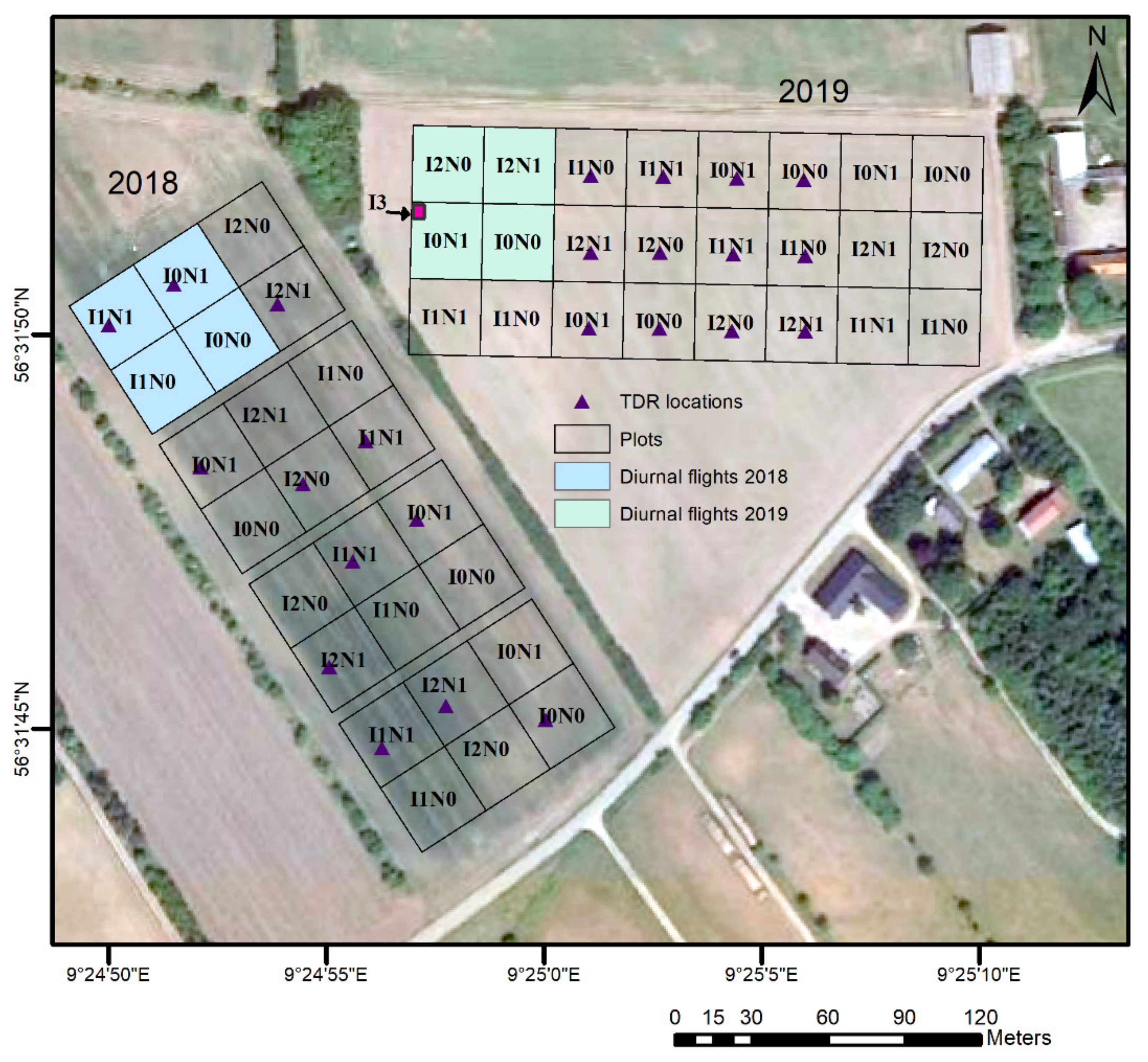
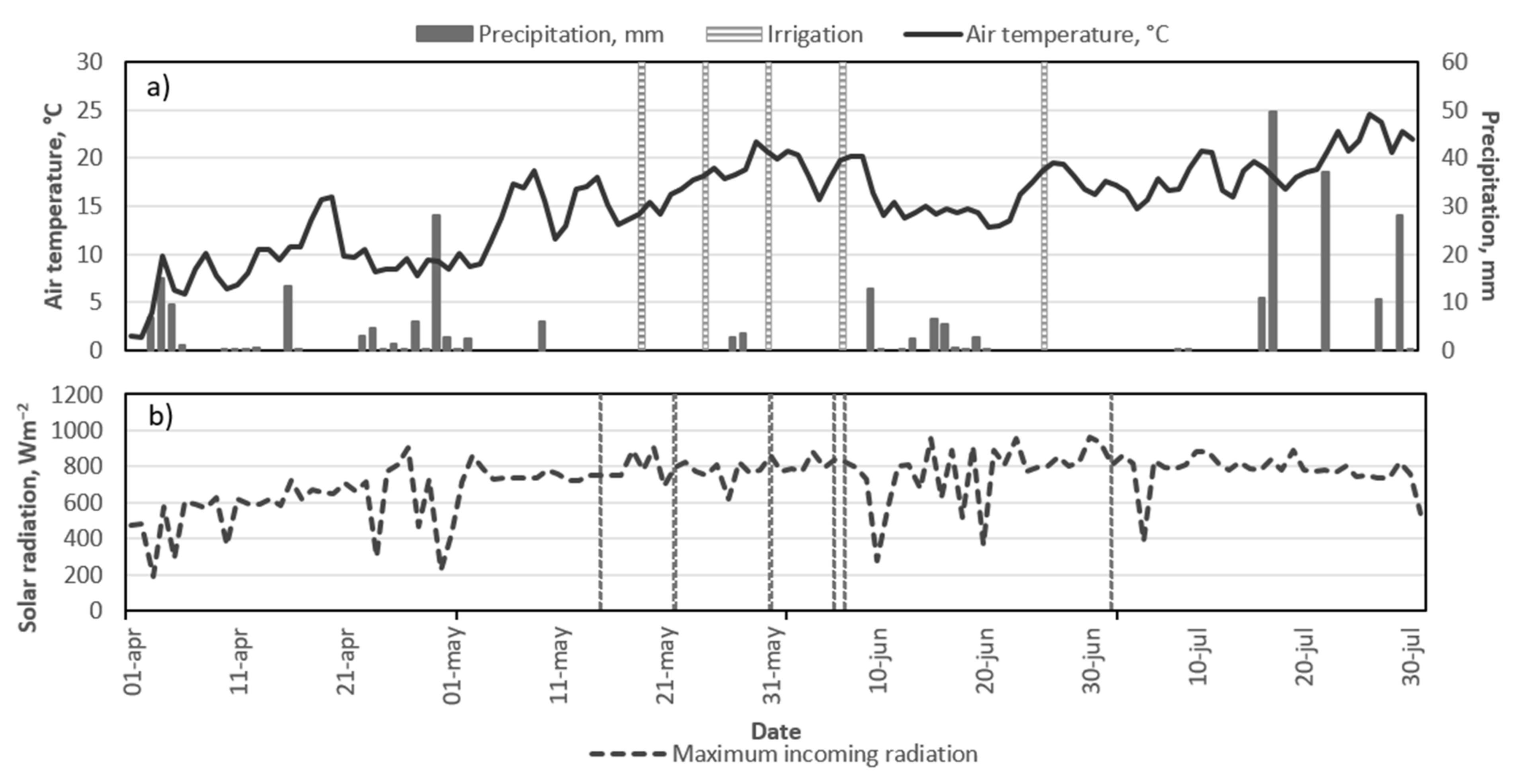
2.1. Experimental Design and Field Measurements

Field experiments with winter wheat (Triticum aestivum L.) were performed in 2018 and 2019 in central Denmark (56°31′59.6″ N 9°24′39.4″ E) on a sand soil (according to the USDA soil textural classification) containing clay, silt, fine and coarse sand of 3.8%, 6%, 32% and 56%, respectively, and organic matter of 2.2% in the topsoil (0–30 cm). The climate is temperate and humid, with cool to cold winters and relatively cool summers. Meteorological variables were measured in 10-min intervals at the nearby station located less than 1 km from the experimental site. Atmospheric conditions at the time of the UAS flight are shown in Table A1 in the Appendix A. The year of 2018 was unusually dry (the 2018 European drought) compared to 2019, which was meteorologically more normal. The winter wheat cv. Hereford was sown on 19 October 2017 and 18 September 2018, and phosphorus (P) and potassium (K) were supplied in early spring according to standard practice. The crop was grown in 30 × 30 m plots, which were replicated four times (Figure A1 in the Appendix A) and arranged in a randomized split-plot design with irrigation as the main plot and nitrogen (N) fertilization as the subplot factor. Irrigation was either minimum (I0), optimum (I1) or full (I2) depending on the measured soil water deficit. However, in 2018, the difference in crop yield between I1 and I2 irrigations was not significant according to the mixed-effects statistical modelling. Further details about the irrigation amounts and dates are shown in Table A2 in the Appendix A. The N fertilization treatment consisted of basic (N0, 90 kg N ha−1) or full (N1, 203 kg N ha−1) irrigation for a target yield of 7 Mg ha−1, split in equal doses in April and May. Crop yields were determined in early August by harvesting four areas of 1.5 × 10 m (15 m2) inside each plot with a Haldrup combiner (Haldrup, Ilshofen, BW, Germany), oven-drying of straw and grain for 48 h at 60 °C and weighing for dry matter (DM) calculation.
Volumetric soil water content during the seasons was measured, covering all treatments by time domain reflectometry (TDR) probes installed vertically to 20 cm, 50 cm and 75 cm depth (Figure A1) [32]. Field capacity (FC) was measured in March after a period with rain and subsequent dry weather for 2–3 days. For the 0–50 cm soil depth, the FC ranged between 66 mm and 100 mm. The plant total available water (TAW) was calculated as the plot-specific value of FC minus a fixed value of unavailable water for the soil type based on Hansen (1976) [33]. The depletion of available water (water deficit) during the season in each plot equipped with TDR was calculated by subtracting the measured soil water content from the TAW. The fraction of transpirable soil water (FTSW) was calculated by dividing the measured soil water content by TAW.
Stomatal conductance (gs) was measured on the youngest fully developed and surface-dry leaf on three plants per replicate with a leaf porometer (Model SC-1, Decagon, Pullman, WA, USA) on both the adaxial and the abaxial surfaces at full sunlight. The LWP was measured after each gs measurement on the same leaf using the pressure chamber method (Soil Moisture Equipment, Santa Barbara, CA, USA) [34].

2.2. Unmanned Aerial System and Acquisition of Multispectral and Thermal Images

The UAS consisted of a Quadrotor DJI Matrice 100 equipped with DJI Zenmuse X3 (12 Mpix true colour RGB), RedEdge multispectral (1.2 Mpix with RGB, red edge and near-infrared bands centered at, 475 nm, 560 nm, 668 nm, 717 nm and 840 nm, respectively) and DRONExpert thermal sensors (640 × 480 pixels). These were used to collect images over the field from May until harvest in August at flight altitude of 50–70 m. The multispectral and the thermal flights were performed separately.

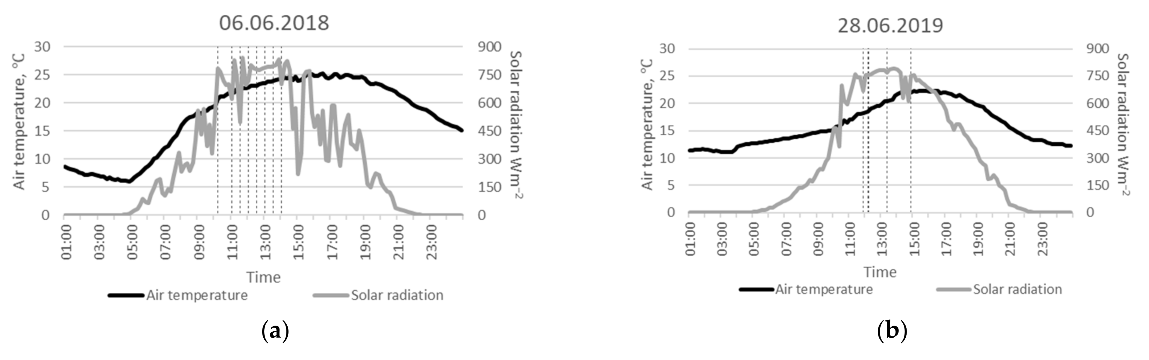
2.2.1. Data Acquisition Times

The seasonal response of winter wheat to treatments was studied in 2018 by engaging the UAS on 5 days, i.e., 15, 22, and 31 May; 7 June; and 2 July. The flights on 31 May and 7 June were conducted during irrigation to assess the reliability of the “wet” threshold of the WDI. The flight on 2 July was conducted closer to the maturity period. In order to study diurnal responses, single-day flights were conducted in June in both years over four plots. In June 2018, six flights were conducted between 10:00 and 14:00 (10:15, 11:00, 11:30, 12:00, 12:30, 13:00, 13:30, 14:00), and in 2019, four flights were conducted between 11:00 and 15:00 (11:49, 12:13, 13:20, 14:49). In both years, the winter wheat was at a comparable growth stage of late flowering/early grain filling (65–75 on the BBCH scale) [35]. The meteorological conditions during the season in 2018, as well as the flight days in 2018 and 2019, are shown in the Appendix A.

2.2.2. Data Processing

The multispectral and the thermal images were processed in Pix4Dmapper software (Pix4D SA, Lausanne, Switzerland) using “Ag Multispectral” and “Thermal camera” mode, respectively. The outputs were high-resolution GeoTIFF images. For all images, radiometric calibration was performed with reference panel for the multispectral data and four reference plates (white, gray, dark gray and black to simulate different temperatures) for the thermal data recorded prior to the flights. For the thermal flights without recorded calibration plates, an equation derived from the previous flight dates was used (y = x*1.428 − 9.193, where x is calibration panel digital number and y is corresponding surface temperature). All images were georeferenced with ground control points fixed in the field, resampled to 10 cm resolution and projected in the same grid and coordinate system (ETRS89/UTM zone 32N, code EPSG:25832).

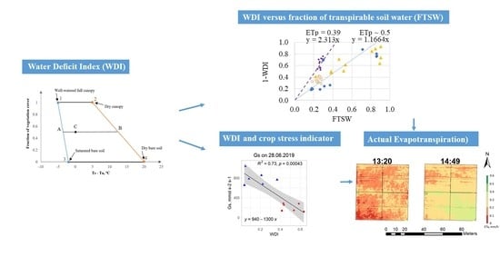
2.3. Calculation of the Water Deficit Index

The VIT trapezoid was used as a reference to distinguish between fully saturated and dry surfaces regarding the fraction of vegetation cover [21]. The method combines the multispectral vegetation index (VI) with the temperature anomaly (surface-air difference) to locate pixels within a trapezoid limited by four baselines points, i.e., (1) well-watered and fully transpiring crop, (2) totally dry and non-transpiring crop, (3) saturated bare soil and (4) dry bare soil. The upper and the lower VI boundaries should be assessed from the maximum and the minimum values of the VI maps. Assuming that surface-air temperature difference (TS − Ta) is a linear function of vegetation cover, the line connecting the well-watered crop to saturated soil forms the “wet” baseline, and the line connecting the non-transpiring crop with dry bare soil forms the “dry” baseline (e.g., Figure 1 with the corresponding values of baseline points in Table 1).
According to Moran et al. (1994), the WDI relates with ETa and ETp according to Equation (Equation (1)):
WDI = 1 ET a ET p = ( T S T A ) min ( T S T A ) mes ( T S T A ) min ( T S T A ) max
where ETa and ETP are actual and potential evapotranspiration rate (mm h−1), respectively; TS and Ta are surface and air temperature (°C_, respectively; and subscripts “min”, “max” and “mes” refer to minimum, maximum and measured, respectively.
For all pixels not fully covered by canopy, the WDI equals to the horizontal distance ratio of a given pixel coordinate (TS − Ta, fc) to the “wet” and “dry” baselines. The equation for the “wet” baseline is x = a + b*y and for “dry” is x = c + d*y, where x is (TS − Ta), y is fc. Thus, it follows for the WDI:
W D I = a + b f c ( T S T a ) m e s c + d f c a + b f c
where fc is fraction of vegetation cover, a and b are slope and intercept of “wet” baseline, and c and d are slope and intercept of the “dry” baseline.
The calculations for points 1 and 2 are identical to those of the CWSI “wet” (Equation (4)) and “dry” (Equation (5)) references, based on determining upper and lower bounds of Ts and implementing the energy balance model shown in Equation (3) [18]:
T s T a = r a R n G ρ C V γ 1 + r c r a Δ + γ 1 + r c r a V P D Δ + γ 1 + r c r a
where ra is aerodynamic resistance (sm−1), Rn is net radiation (Wm−2), G is soil ground heat flux (Wm−2_, Cv is volumetric heat capacity of air (1200 J °C−1), ρ is air density (kg m−3), VPD is vapor pressure deficit (kPa), γ is the psychrometric constant (0.067 kPa °C−1), ∆ is the slope of saturation vapor pressure curve (kPa °C−1) and rc is canopy resistance to vapor transport (s m−1). The equations for these variables are shown in the Appendix B.
For a full covered non-stressed canopy that transpires near to or at potential level and therefore has minimum rc = rcp (VIT point 1), the following Equation applies:
T s T a 1 = r a R n G ρ C V γ 1 + r c p r a   Δ + γ 1 + r c p r a V P D Δ + γ 1 + r c p r a
For a full-covered and stressed, i.e., non-transpiring canopy with maximum rc = rcx (VIT point 2), the temperature anomaly equals:
T s T a 2 = r a R n G ρ C V γ 1 + r c x r a Δ + γ 1 + r c x r a VPD Δ + γ 1 + r c x r a
For saturated bare soil, there is no canopy resistance, i.e., rc, rcp and rcx in Equations (6) and (7), respectively, equal zero (VIT point 3). However, there is resistance to heat transfer in the boundary layer immediately above the soil surface (rs) that should be added to ra [19] according to:
T s T a 3 = ( r a + r S ) R n G ρ C V γ Δ + γ VPD Δ + γ
Finally, dry bare soil conditions (VIT point 4) are represented by Equation (4). Due to the highly variable conditions present for dry soil mixed with fveg, Rn and G should be calculated separately, whereas ρ can be omitted:
T s T a 4 = ( r a + r S ) R n d r y   s o i l G ( d r y   s o i l C V
As a measure of fveg, the Normalized Difference Vegetation Index (NDVI) can be used due to its high correlation with fveg [25].
Net radiation (Rn) is the balance (difference) between incoming solar radiation Rs (global radiation) and outgoing (emitted and reflected) radiation in the shortwave and longwave regions. Rn can be estimated as a fraction of Rs, e.g., 68% for cereal crops [36].
When measured, Rn refers to a vegetated surface well supplied with water. Moran et al. (1993) [21] pointed out the importance of caution when using identical Rn for bare soil. In order to improve calculations for dry bare soil conditions, Rn was calculated by the Stefan-Boltzmann law, iterating the soil temperature:
R n = 1 α R s ε s   σ T S 4 + ε a σ T a 4
where Ts in this equation is soil temperature (°C); α is albedo (~0.12 for dry bare soil derived from UAV images); σ is the Stefan-Boltzmann constant σ = 5.67*10−8 [W⋅m−2⋅K−4]; and εs and εs is the emissivity of soil and air, respectively (see Appendix B).
The energy used for soil heating (G) is positive for warming and negative for cooling, and estimates typically range around 10% of Rn, although this value may be very different for full cover and bare soil conditions. Therefore, in the present study, G was calculated with regard to a fraction of vegetation cover following Kustas and Daughtry (1990) [37]:
G = 0.325 0.208   N D V I   R n
where the NDVI was fixed to 0.9 for full-cover winter wheat and 0.2 for bare soil according to the field image estimates.
Further details on the energy balance parameters calculations are provided in Appendix B.

2.4. Calculation of Seasonal and Diurnal Evapotranspiration

According to Allen et al. (1998) [27], ETp is estimated by ‘correcting’ the reference evapotranspiration (ET0) of a well-managed grass with a coefficient (Kc) that integrates crop and climate characteristics, i.e., ETp = Kc*ET0. In order to find ETa where the crop canopy is not full and drought stress may occur, a dual Kc model can be used by explicitly considering crop transpiration and soil evaporation:
E T a = E T 0   K c b K s + K e
where Kcb is basal crop coefficient, Ks is the drought stress coefficient and Ke is the evaporation coefficient of the bare soil. The units of ETa and ET0 are mm h−1, and the latter was calculated by the Penman-Monteith Equation [27]:
E T 0 = 0.408 Δ R n G + γ 37 T a h r + 273 u 2 e 0 T a h r e a Δ + γ 1 + 0.34 u 2
where Ta(hr) is the mean hourly air temperature (°C), u2 is the wind speed at 2 m height (m s−1), e0Ta(hr) is the saturation vapor pressure at the temperature Ta (kPa) and ea is actual vapor pressure [kPa].
The crop coefficient for winter wheat in Denmark during the mid-season varies from 1.09 to 1.15 depending on the growth conditions [28]. In this study, the mid-season crop coefficient Kcb full (at maximum plant cover and height) was assumed to be 1.1. For the areas without full crop cover, Kcb was calculated by the following formula:
K c b = K c   m i n + K c b   f u l l K c   m i n f c 1 1 + h
where Kc min is minimum Kc for the bare soil assumed to be 0.15, fveg is the fraction of soil surface covered by vegetation [0.01–1] and h is plant height (m).
According to Gutman and Ignatov (1998) [38], fveg can be calculated from the NDVI:
f c = N D V I N D V I m i n N D V I m a x N D V I m i n
where NDVImin and NDVImax are the minimum and maximum NDVI values corresponding to bare soil and full vegetation cover, respectively.
The drought stress coefficient Ks was calculated using the WDI similarly to Tang, Han and Zhang (2019) [25] who used CWSI:
K s = 1 W D I
The evaporation fraction from bare soil (Ke) is highly influenced by the fraction of soil covered by vegetation, i.e., Ke depends on fveg [25] and is highly dependent on soil moisture in the top layer. In the absence of available water, Ke will be close to 0. Thus, it is possible to calculate Ke using the WDI:
K e = 0.25 1 f c 1 W D I
All calculations of the VIT trapezoid and ET were conducted for each flight at a half-hourly timestep at the time of the UAS flight. Further details on the parameter calculations are provided in Appendix B.

2.5. Calculation of Fraction of Transpirable Soil Water

The FTSW is the ratio between available and total transpirable soil water, with the latter being equal to the difference between FC and WP. The relation between the rate of transpiration ETa/ETp (and, correspondingly, 1-WDI) and the FTSW can be conceptualized according to Raes et al., (2009) [39] as a suite of curves differing in the level of ETp [27]. At higher ETp, a larger FTSW is needed for the crop to avoid drought stress, whereas at lower ETp, the crop can thrive at smaller FTSW. Whereas these studies considered daily values of these variables and relations, in the current study, the scheme was adopted to hourly values relevant to the diurnal WDI analysis. Analogous to Raes et al. (2009) [39], Equation (16) was iterated to fit the constant a, allowing the estimation of the FTSW from the WDI and the validation of the WDI:
1 W D I = c + a × E T p E T m i n   × F T S W
where c is the slope of the curve with lowest ETp (ETmin). Equation (18) can be rearranged to isolate FTSW:
F T S W = 1 W D I c + a × E T p E T m i n  
However, caution is needed when using Equations (16) and (17). For instance, dry soil receiving a few millimeters of rain does hold freely available water, allowing a crop to transpire at its potential rate despite FTSW being small for the entire root zone.
Using the approach to estimate FTSW makes it possible to calculate the amount of water needed to reach field capacity, i.e., the Soil Water Deficit (SWD, mm) as:
S W D = F C F T S W T A W

2.6. Statistical Analyses

Linear regression modelling was used to assess the relation between the WDI and soil water content and SWD. The coefficient of determination (R2) was calculated to assess the strength of the relationships at 95% significance level. The daily WDI maps for the 2018 season were also correlated with the measured soil water content and the estimated SWD. For these correlations, mean WDI per plot was used. Furthermore, WDI was validated by comparing measured WDI values to modelled ones according to Equation (16) using FTSW.
The diurnal WDI maps for 6 June 2018 and 28 June 2019 were also correlated with LWP and gs measured during the flights. For these correlations, mean WDI of 1 m2 around the measurement locations was used. All image analysis was conducted in ArcMap (10.6.; ESRI, Redlands, CA, USA), whereas WDI, evapotranspiration maps and statistical evaluation were performed in R (ver. 3.5.1; R Core Team, 2013).

3. Results

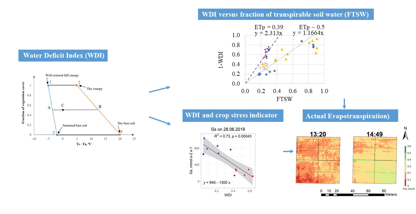
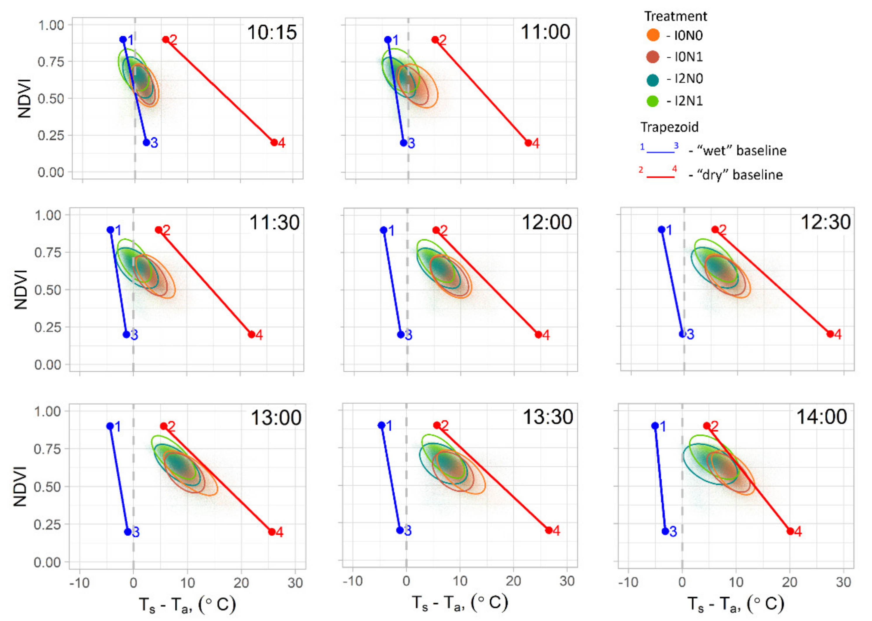
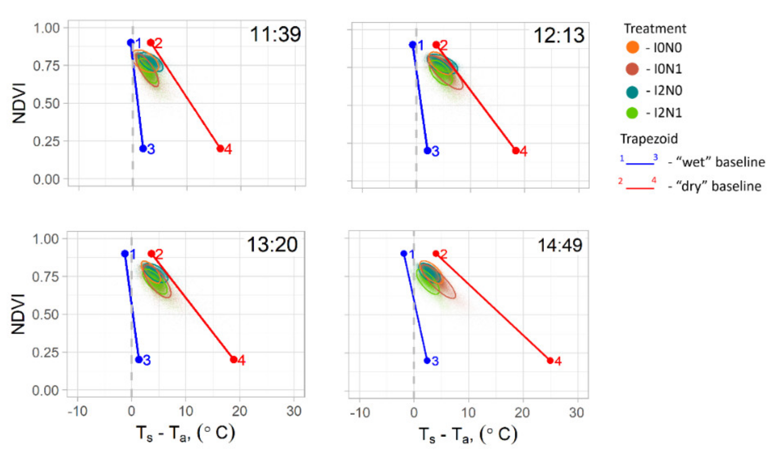
3.1. Vegetation Index/Temperature Trapezoid on Seasonal and Diurnal Scale

Parameterization of the VIT trapezoid for the 2018 season and for the diurnal flights in 2018 and 2019 is shown in Table 1. The mean “wet” reference for the crop-air temperature difference (VIT point 1) in 2018 was around −5 °C, while in 2019, it was close to 0 °C due to higher humidity (more than 60% on 28 June 2019). Lower relative humidity and higher wind speeds results in larger difference between the “wet” and “dry” baselines. The typical “dry” baseline for the crop (VIT point 2) was 4–5 °C higher than Ta (Table 1). The saturated bare soil-surface temperature difference (VIT point 3) was slightly higher due to the higher surface resistance and less transpiration compared to evapotranspiration. The largest variation in the temperature difference was seen for the “dry” soil conditions (VIT point 4) as, in the absence of available water vapor, surface temperature is defined only by accumulated incoming radiation and can be greatly reduced by wind. Therefore, under low wind speed, the aerodynamic resistance ra of soil surface to water vapor and its heat gradually increases and vice versa. The temperatures of 13 °C (on 22 May 2018, Table 1) and 25 °C (on 06 June 2018 at 12:30, Table 1) above Ta correspond to conductions with higher and lower wind speed conditions, respectively. The iteration of Rn for VIT point 4 (Equation (8)) resulted in more reasonable values of T, which were otherwise underestimated, resulting in many measurement points positioned left of the dry boundary outside the trapezoid.

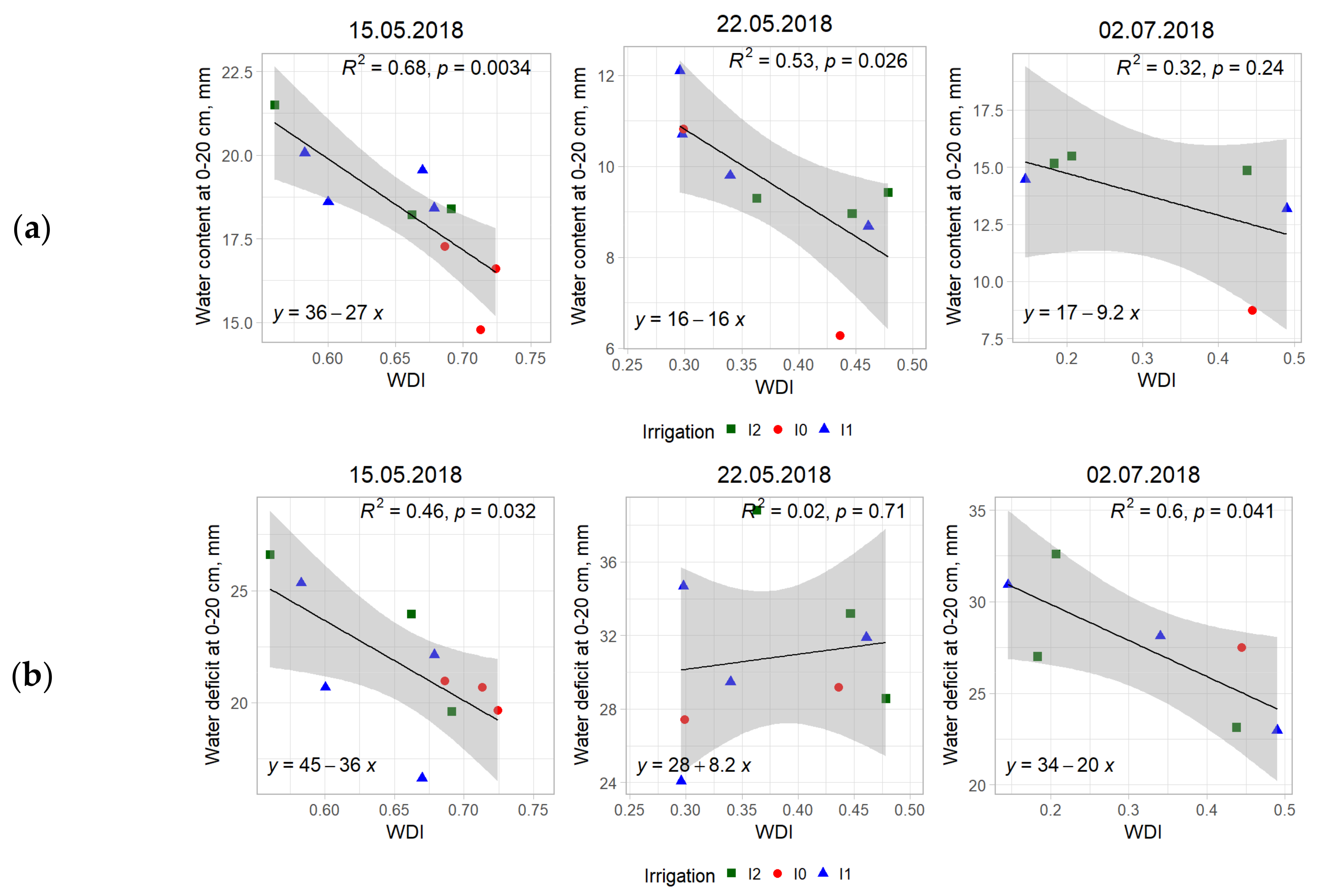
3.2. Water Deficit Index at Seasonal Scale and Correlation to Field Data

The VIT trapezes developed by the seasonal data in 2018 are shown in Figure 1 and the associated NDVI and WDI maps are shown in Figure 2. Due to the high evaporative demand during May and June 2018, it was not possible to follow the planned irrigation schedule. Consequently, treatment I0 was minimally irrigated, while I1 and I2 treatments suffered periodic drought stress despite irrigation (Appendix A, Table A2). The NDVI distribution indicates high variability in fc, i.e., mixed pixels and less distinct differences between treatments, which was expected with the planned irrigation schedule (Figure 2a). The flight on 22 May was conducted after irrigation. Thus, the winter wheat had lower WDI values, and most pixels were located close to the ‘wet’ reference in VIT (Figure 1). However, in mid-May, the winter wheat already showed signs of drought stress, as indicated by the low NDVI and high WDI (Figure 2), due to the prolonged dry spell from the end of April and throughout May, as well as limited irrigation. The grain yield in 2018 was low for all treatments, i.e., only 2.7 Mg ha−1, 3.5 Mg ha−1 and 3.2 Mg ha−1 for I0, I1 and I2 respectively, which is almost half compared to the corresponding 2019 values of 5.9 Mg ha−1, 5.9 Mg ha−1 and 6.0 Mg ha−1.
On 31 May 2018, the flight was conducted when one-third of the field was already irrigated the day prior to the flight (right row) one-third of the field was irrigated the same morning as the flight (left row) and one-third of the field was not irrigated yet (middle row) (Figure 2b). The already irrigated plots transpired below potential level, thus showing early stress symptoms under the prevailing high evaporative demand. On 7 June 2018, the irrigation machine was present in the field during the flight. Taken as a whole, in 2018, insufficient irrigation under drought made treatment differences in yield rather small according to the analysis of variance (results not shown).
There were significant but medium-strength correlations between the WDI and topsoil water status, with mostly stronger correlation to soil water content (SWC) at 0–20 cm compared to the soil water deficit (SWD). The R2 values were 0.68 on 15.05, 0.53 on 22.05 and 0.32 on 02.07 for SWC, and 0.46 on 15.05, 0.02 on 22.05 and 0.6 on 02.07 for SWD (Figure 3).

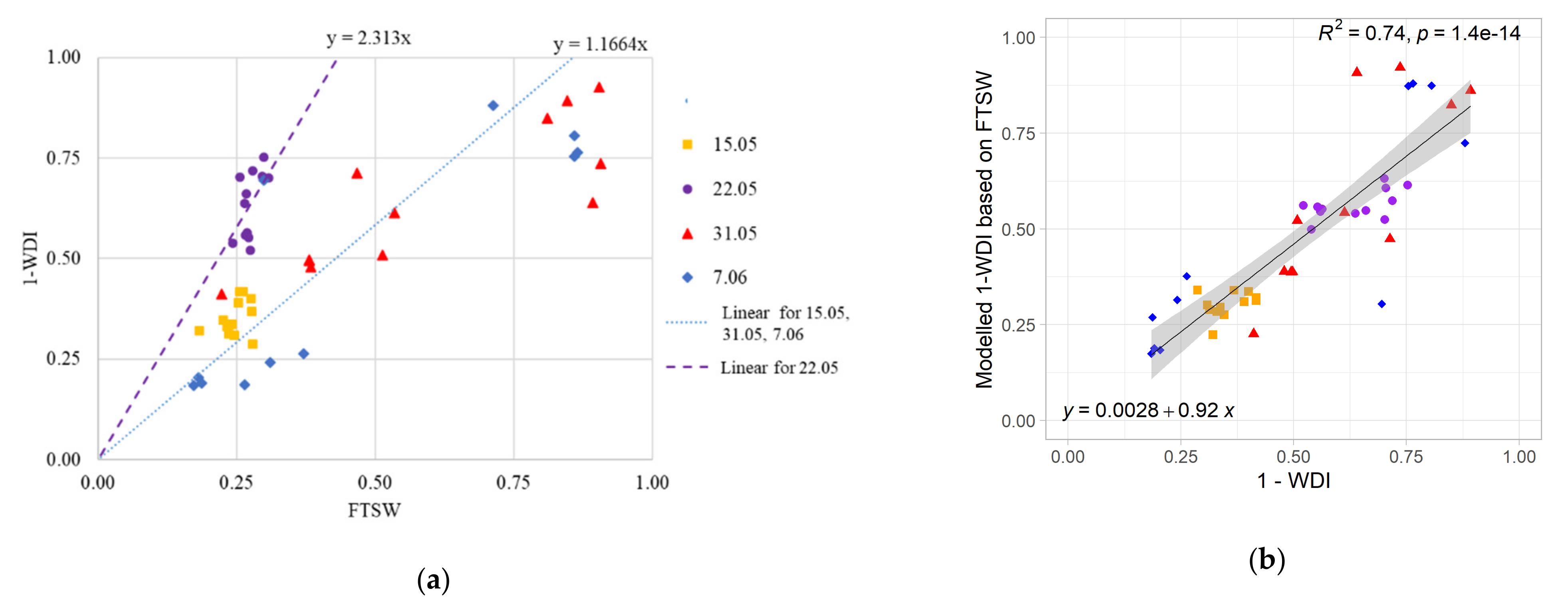
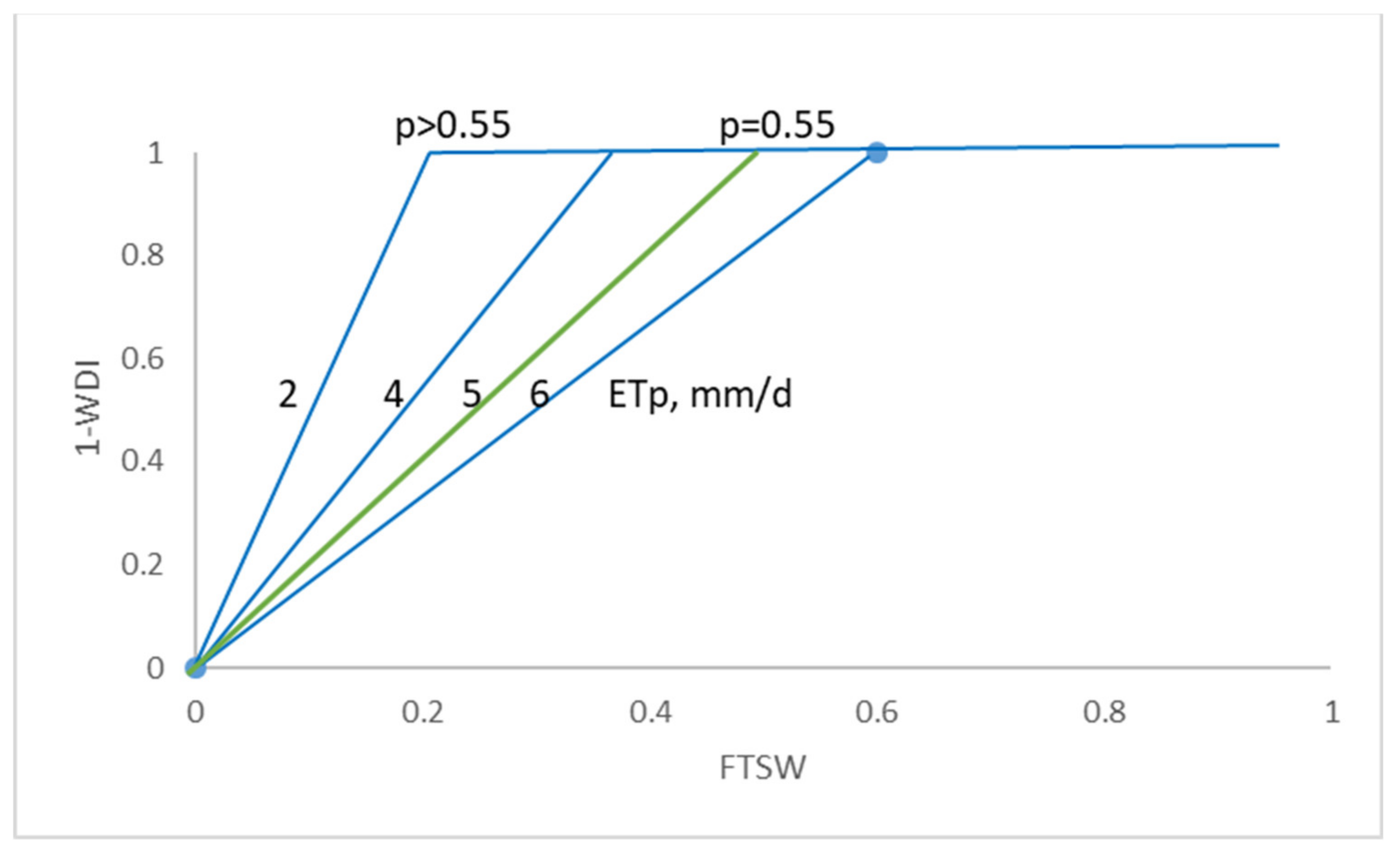
3.3. Relation between the WDI and the Fraction of Transpirable Soil Water and ETp

The relation between relative transpiration rate, i.e., ETa/ETp as predicted by (1-WDI), and FTSW in the 0–50 cm soil depth, which comprises the majority of the root zone, is shown in Figure 4a. It was possible to describe the relationship with one linear equation for the data measured on 15 and 31 May and 7 June 2018, which had similar ETp values of ca. 0.45 mm h−1. However, the data from 22 May 2018 had a larger slope, which is likely related to the lower ETp that day. Based on Figure 4a, the relation for the lowest ETp (ETmin = 0.39 mm h−1 and slope c = 2.31) is shown in Equation (17), whereby an optimal value of a = 3.31 was found by iteration. Using these parameters in Equation (17), the values (1-WDI) were derived from the measured FTSW, which fitted quite well with the average (1-WDI) per plot derived from the thermal imagery (Figure 4b).

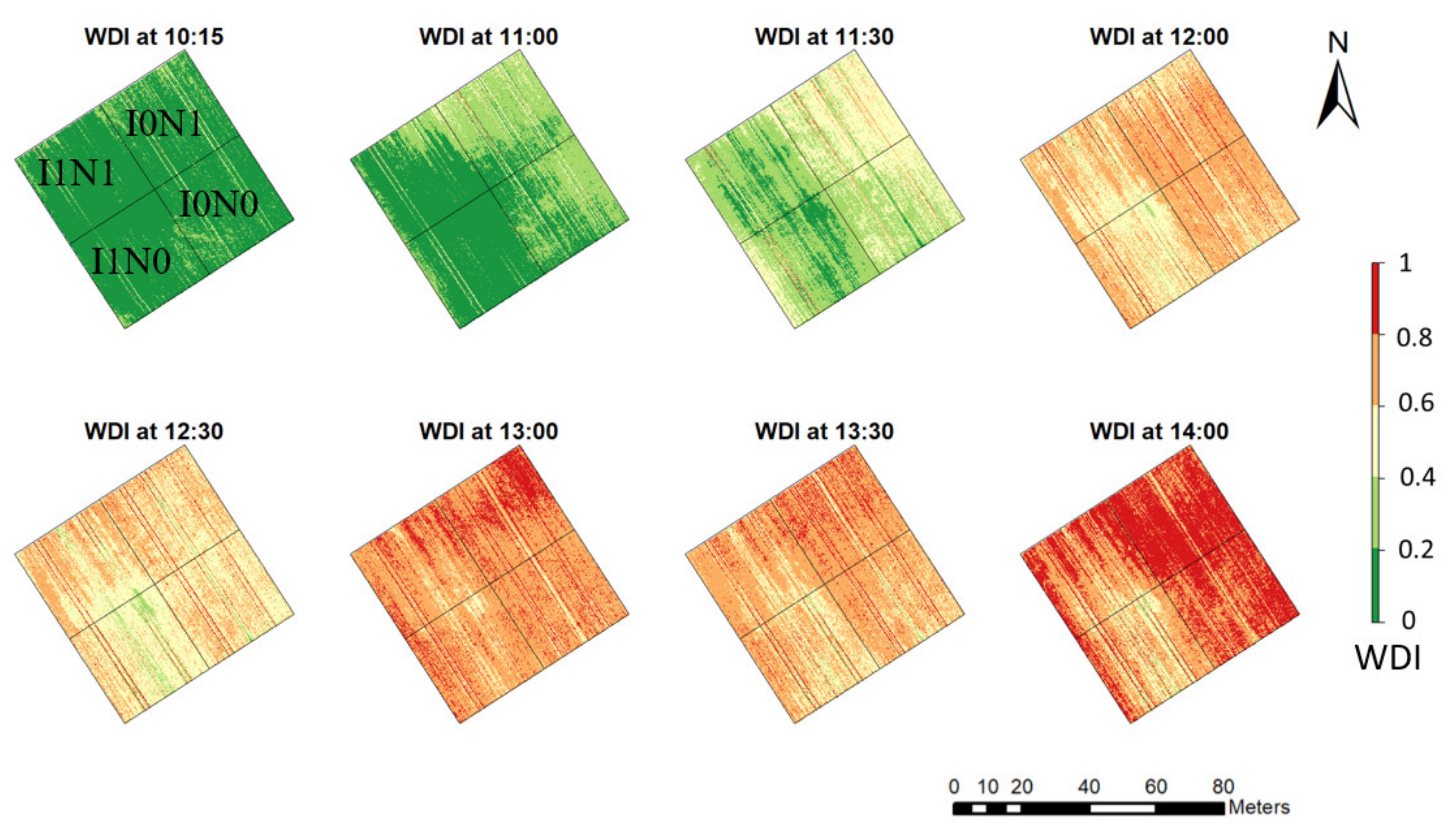
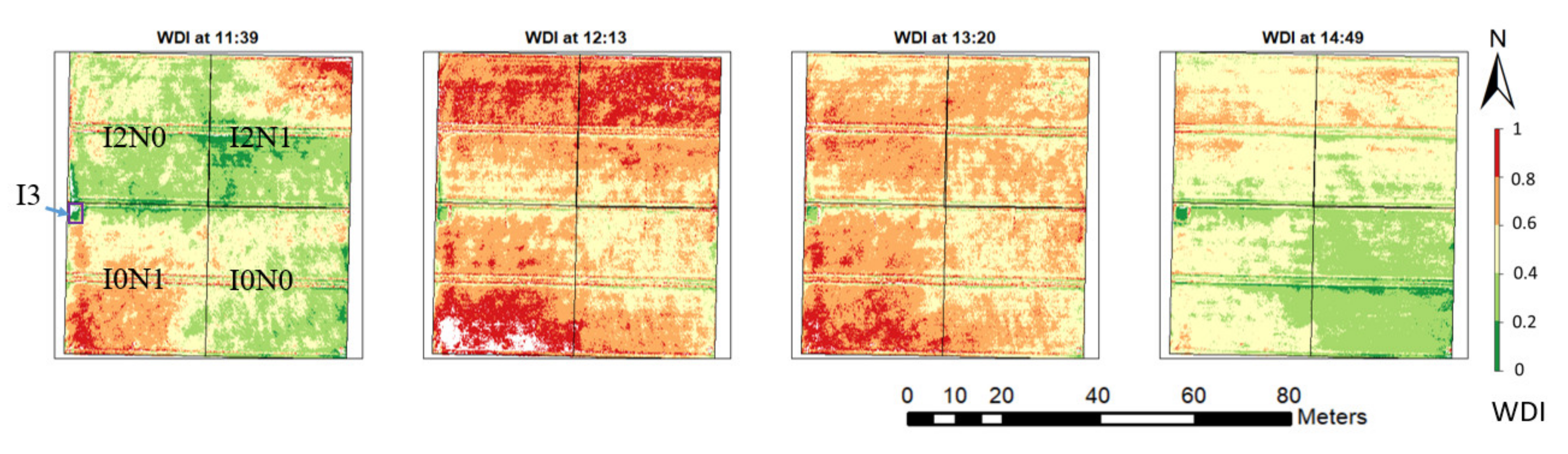
3.4. Modelling Water Deficit Index at Diurnal Scale

The VITs derived by the diurnal data from 2018 and 2019 are shown in Figure 5 and Figure 6, respectively, and detailed WDI maps for these diurnal flights are shown in Figure A5 and Figure A6 in the Appendix C. In 2018, for the morning flight (10:15), certain pixel values were located outside the trapezoid, i.e., being “wetter” than the non-stressed baseline. These differences were likely due to free water present on the leaves as dew formed during the night, which was confirmed by relative humidity of almost 100% according to the meteorological data. As water evaporated, the WDI started to depict the actual plant water status, implying that the thermal data acquisition should not be conducted in the morning to ensure the absence of free water otherwise leading to skewed WDI. Similar trend was observed in 2019 with WDI increasing at noon hours.
In both years, there was no consistent response of LWP and gs to treatment (Figure 7). In 2018, the average LWP was −2.35 and −1.53 MPa for plots under low and higher irrigation, respectively, while the corresponding gs was 101 and 160 mmol m−2 s−1. In 2019, a small plot (3 × 2 m) irrigated separately the day before the flight showed average LWP of −1.11 MPa compared to −1.43 MPa for the non-irrigated plot. The corresponding gs was more distinct, with 559 and 319 mmol m−2 s−1, respectively. The WDI was significantly but weakly to moderately correlated with the measured leaf physiological parameters, with stronger correlation for gs compared to LWP (Figure 7).

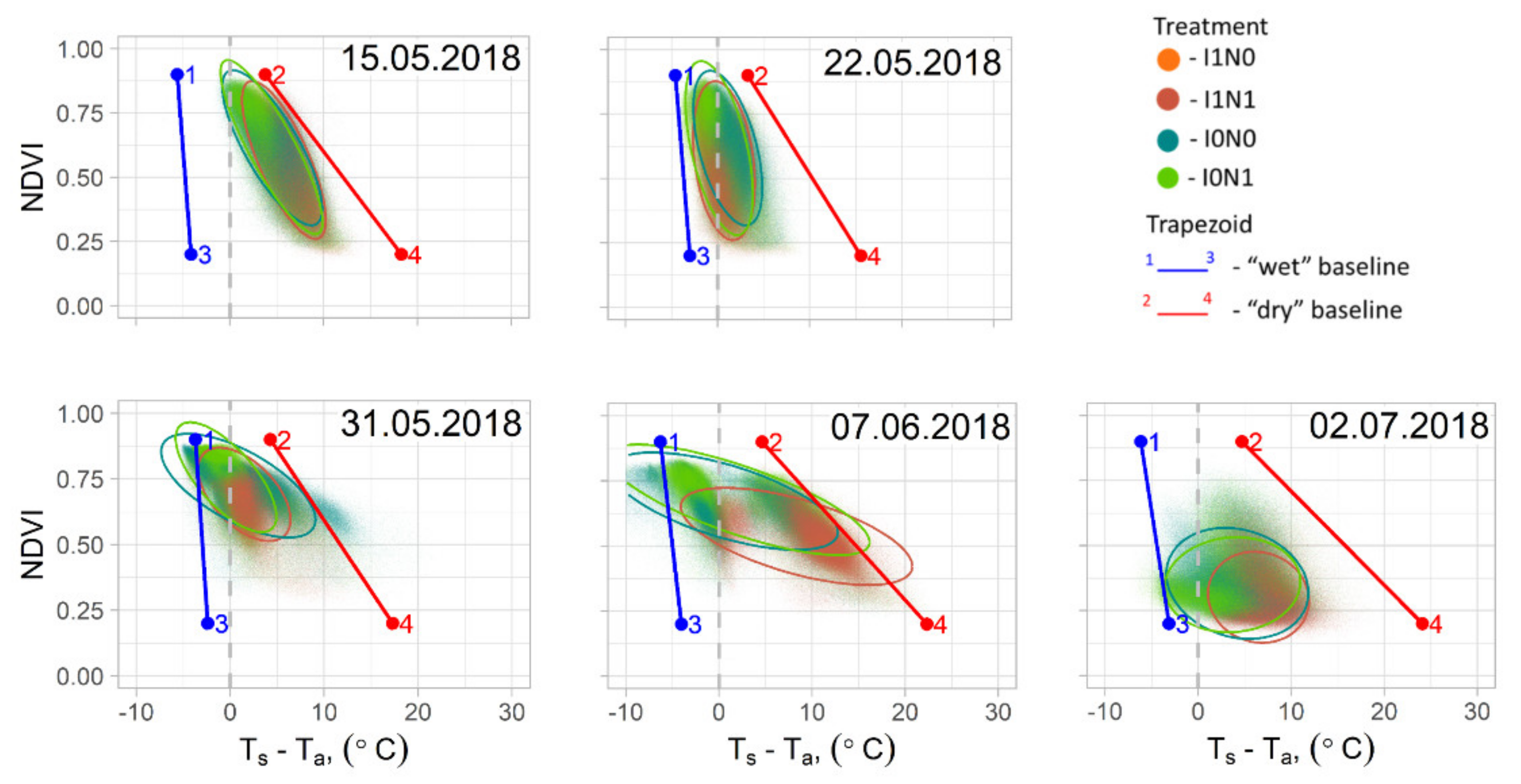
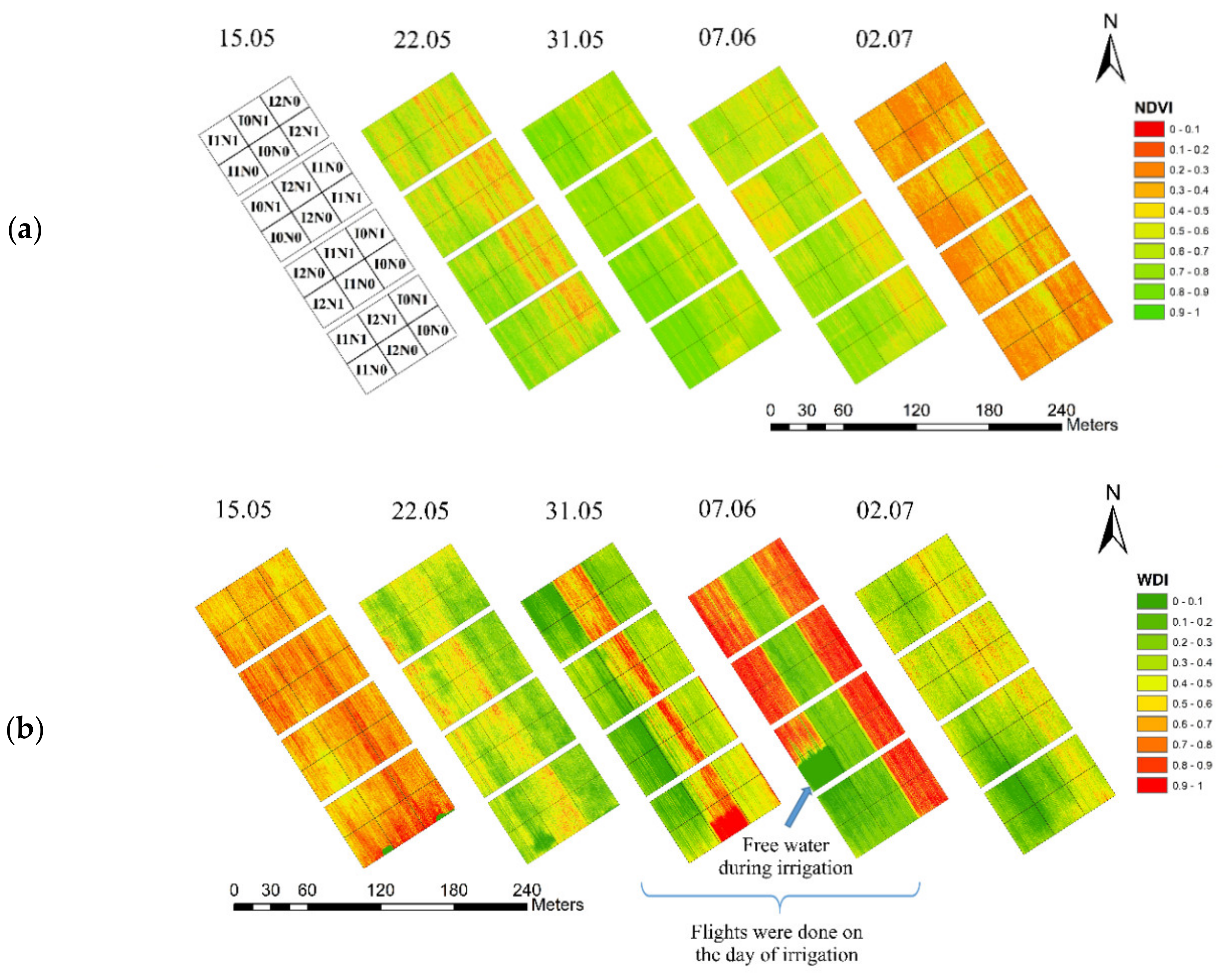
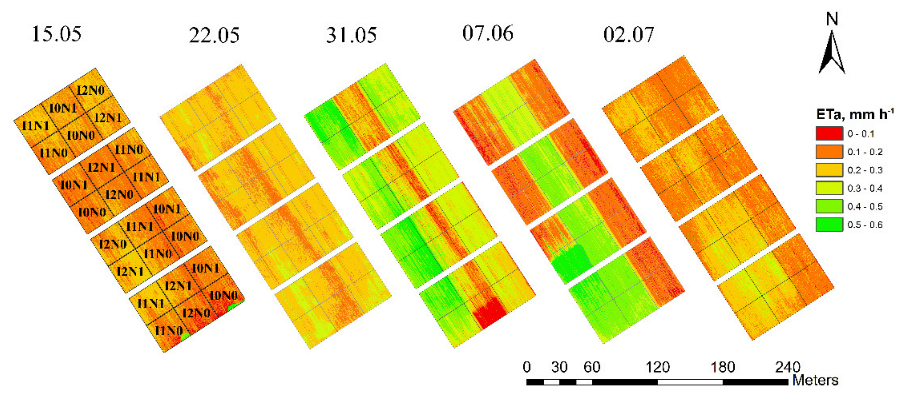
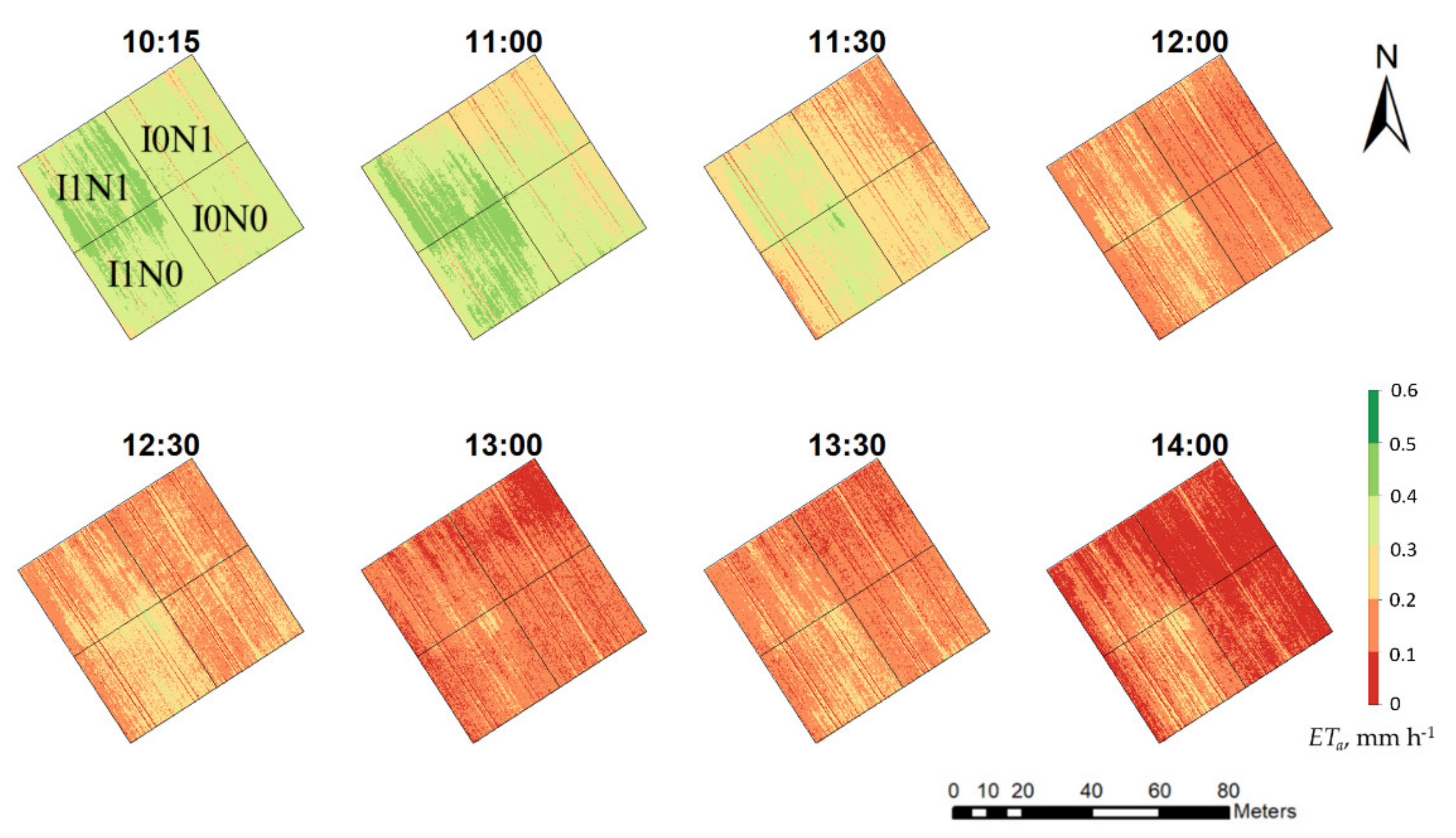
3.5. High-Resolution Mapping of Actual Evapotranspiration at the Seasonal and Diurnal Scale

The spatiotemporal distributions of ETa for the winter wheat using the dual Kc approach (Equations (10)–(15)) and the derived WDI for the 2018 season are shown in Figure 8 and for the diurnal scale in Figure 9 and Figure 10 for 2018 and 2019, respectively. On most days, ET0 at the time of the flight was around 0.5 mm h−1 (Table 1), with the lowest value of 0.35 mm h−1 on 22 May due to the lower incoming radiation at the time of flight. Except for the flights performed during irrigation, ETa did not exceed 0.3 mm h−1, which pointed to low water availability and transpiration even for the full irrigation treatment. Diurnally, ETa decreased with time during the day and certain areas in the plots. Lower soil water deficit indicated a ‘recovery’ in evapotranspiration rate in the afternoon (Figure 9 and Figure 10), suggesting that the ETa rate is not constant during the day and irrigation planning from a single mid-day image may be complicated.

4. Discussion

4.1. Seasonal Dynamics of the Water Deficit Index and Correlation to Soil Water Status

Monitoring and managing drought on time is important to allow crop physiological recovery, whereas delayed response is associated with irreversible damage and yield loss [40]. The spring of 2018 was exceptionally warm and dry, and crop yields were inevitably reduced by almost half (possibly also due to heat stress) despite irrigation during the season in the I1 and I2 treatments. Modelling the relation between the WDI and FTSW in the root zone was conducted to validate the ability of the WDI to estimate the FTSW and describe the rate of ETa (Equations (16) and (17)). The model has potential to be used both ways, either deriving the FTSW using the WDI or vice versa, depending on aim and available measurements. The WDI derived from thermal imagery was significantly correlated to the WDI modelled from the FTSW (R2 = 0.74), and knowing the FTSW along with soil FC and WP allows the assessment of the exact amount of water needed for irrigation (Equation (17)). The FTSW level needed for a crop to transpire at a potential level depends on the ETp. Therefore, future studies may explore larger variations of ETp and soil water contents by conducting UAS flights over longer periods or studying different crop systems. As noted earlier, the FTSW estimation based on WDI measurements can only be assumed to be valid during prolonged drying periods as was the case in this study during 2018. This is because a minor rainfall, which does not bring the FTSW to unity, is expected to bring the WDI to 0 due to the presence of easily available water in the root zone.
It should be mentioned that all calculations were conducted at the time of the flight in 30 min and are expressed at the hourly scale (e.g., ETa in mm h−1), as the typical flight duration was 20 min and mean meteorological conditions for a 30-min timeframe are the most representable. Soil moisture was the sole daily variable either measured with TDR (not exactly overlapping flight time/hour) or calculated by simple soil water balance [33] when TDR readings were done some days apart. It was assumed that WDI and ETa seasonal measurements to represent their values at the time of a flight as reliable upscale was neither possible nor objective of the study.
Under prolonged drought, winter wheat fastens its development, shortens its season, but also reduces ETa [7]. It was possible to distinguish between an irrigation that was done 1 day before the flight and the same-day irrigation (31 May 2018; Figure 2b), as winter wheat irrigated the day before already showed a higher WDI than wheat irrigated on the same day. Similarly, on 7 June 2018, when the flight was performed during irrigation, plots that were irrigated earlier on the same day already showed signs of drought stress. The WDI was higher than 0, hinting that soil at field capacity could not even fulfill the evaporative demand in this hot and dry season on the coarse sand. This has important implications for the use of WDI and it shows its dependence on soil water status (the “wet”-“dry” soil baseline). Colaizzi et al. (2003) and Köksal, (2008) [24,41] also found a relation between WDI and soil moisture. However, the WDI variation within each plot was high, and the mean WDI resulted in medium correlations to the point TDR measurements (Figure 3). Wang et al. (2018) [42] pointed out that, under dense vegetation, canopy temperature is better correlated with root-zone soil moisture than with the surface layer water content. Therefore, WDI areas with less crop cover represent the availability of the water in the topsoil and do not reflect the deeper soil water status. In this study, there was significant correlation only to the topsoil moisture in 2018 with R2= 0.68 on 15 May for water content and R2=0.6 on 2 June for water deficit. Hoffmann et al. (2016) [19] found a similar relation of surface-air temperature difference to soil water content, with R2 values between 0.56 and 0.83. Other soil types and soil water conditions at various depths need to be explored to search for stronger correlation or a proxy for ETa under different conditions.

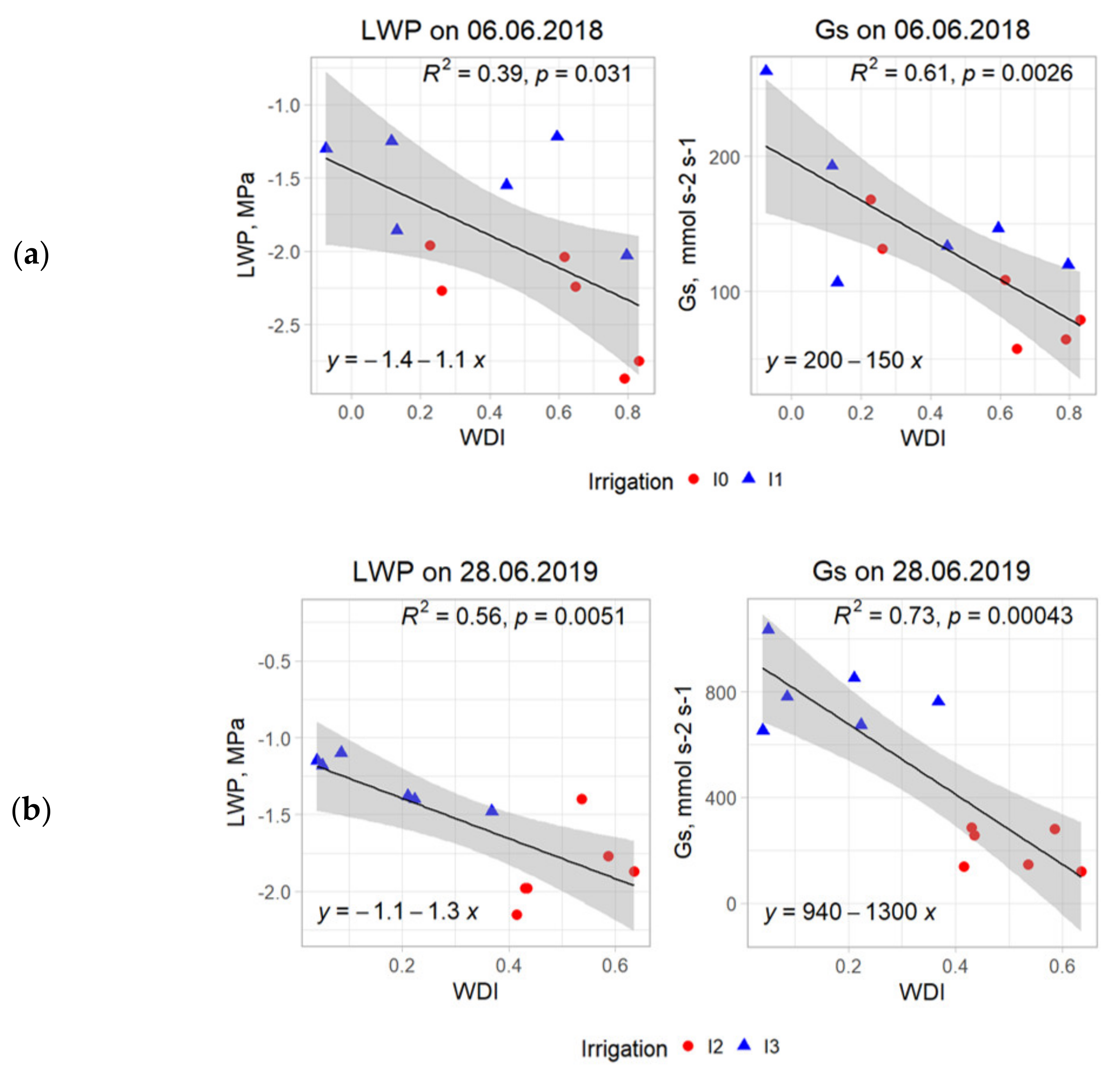
4.2. Water Deficit Index on the Diurnal Scale and Correlation to Leaf Water Status

On 6 June 2018, relative humidity during the night was close to 100%, which led to dew accumulation on the winter wheat leaves and lowered the temperature compared to the VIT estimation (Figure 5). This can also be explained by the ability of the plant to replenish water during the night from the deeper levels of the soil profile. After 11:00, as the surface temperature increased, it gradually moved the pixels of the VIT range toward the “dry” WDI baseline. This led to the conclusion that UAS images should not be acquired too early in the day (e.g., 10:00) because the presence of dew on the surface of the plant may skew the WDI toward less stressed. Areas with winter wheat having more water available for transpiration recovered faster in the afternoon. In contract, plants water-limited areas remained stressed for a longer time (Figure 5 and Figure 6).
The UAS flights are typically performed at or around noon to assess plant transpiration [43]. As shown in Figure 5 and Figure 6, plants demonstrated stress between 12:00 and 13:00, likely due to the high air temperature triggering reduced transpiration to avoid high water loss. In addition, lower wind speed contributed to higher rs − aerodynamic resistance of heat and water vapor from the surface into the air above the canopy, leading to an increase in Tc and vice versa. As the afternoon progressed, plants that are less stressed started to recover, while the others showed high levels of stress as canopy pixels moved in the VIT space from the “dry” toward the “wet” baseline (Figure 5 and Figure 6). The observed “partial afternoon recovery” (decrease of the WDI at 14:50, Figure A5 and Figure A6 in the Appendix C) follows the theory that plants rehydrate during the afternoon and night. Transpiration starts in the morning, leading to lower plant water potentials and, in turn, the partial closure of the stomata. At some stage during the afternoon, soil water uptake exceeds transpiration due to high water potential gradient between plant and soil, leading to the partial recovery of transpiration and hence lower WDI as simulated by Jensen et al. (1993) [13] and shown in Figure 7 for drought-stressed barley. Therefore, afternoon UAS acquisition may be useful to find areas in the field that have higher irrigation demands.
Significant correlation to gs with R2 up to 0.73 demonstrates the ability of the WDI to detect early crop drought stress signals (Figure 7). Stomatal closure due to increased temperature and limited water supply limits ETa and increases Tc. The diurnal changes in Tc are directly caused by plant transpiration [44]. In addition, gs is one of the common plant physiological indicators used to determine crop water status [13]. In 2018 and 2019, all treatments had low gs values of around 200 mmol m−2 s−1 (Figure 7a,b) compared to plot that was irrigated the day before the measurements, with gs values up to 900 mmol m−2 s−1 (Figure 7b) indicating drought stress and limited transpiration in plots with low gs. The gs and crop transpiration may vary between different cultivars of the same species [7]. Therefore, the WDI method should be further investigated as a potential phenotyping tool.
Some studies have suggested the possibility of using Tc and derived thermal indices to distinguish between water status and the predicting index from LWP values [45]. It may be difficult to derive LWP using the WDI due to the different dynamics in LWP diurnal pattern depending on the weather conditions and stress level [46]. In this study, significant but weak correlation of WDI to LWP was found (maximum R2 = 0.56). This can be attributed to the spatial heterogeneity in the crop growth which is commonly seen in the field under same management conditions, i.e., the subtle spatial variation.

4.3. Links between Evapotranspiration and Water Deficit Index

Reference evapotranspiration calculated for full-crop conditions must be adjusted for fc analogous to the WDI (only assuming that the relationship between crop and soil is linear). This was achieved using the dual Kc approach according to Allen et al. (1998) [27], which accounts for both crop transpiration and soil evaporation with regard to canopy cover and stress index. The two-source approach provides high ETa estimation accuracy [47], especially when the canopy is less dense and the soil evaporations has a larger contribution to ETa. As it can be seen from the diurnal responses (Figure 9 and Figure 10), the ratio of ETa to ETp during the day was not constant as the WDI values changed from the morning to the afternoon. The change in the ETa/ETp ratio during the day may add uncertainties to quantifying crop water demand if using a single-shot image. It may complicate the use of the WDI for irrigation scheduling if the time of the flight for drought stress detection is not chosen correctly. On sandy soils and even under ample irrigation, water availability is limited for the noon hours when ETp reaches higher values. Previous studies have upscaled daily ‘single-shot’ images acquired by UAS or satellites in order to derive daily ET products, which may lead to different results depending on the time of day and instantaneous meteorological conditions [48], therefore accounting for the change in ET fraction improved by the upscaling [49]. In this study, the relation of th WDI to the FTSW clearly shows the potential use of WDI in ETa calculations since the FTSW can be used to calculate Ks, as shown by Equation (10) [27]. Future studies should assess the time upscaling issue to improve estimation of crop water demand. Further refinement of the ETa calculations may be possible using nonlinear boundaries for the “wet” and “dry” baselines [50].
On the seasonal timescale, the WDI depicts the daily crop growth and supports identifying areas in the field that are prone early drought stress, prompting irrigation on a particular day. On the diurnal scale, the WDI depicts the crop behavior more precisely, which can provide more insight on the crop status and water need. Studies has revealed a ‘crosstalk’ between the drought stress and diurnal regulation of a range of genes differing in the vegetative and reproductive stage of crop development (e.g., [11]). At high ETp, sandy soils may not be able to fulfill crop demand to resupply water during noon heat wave. It may happen even if there is sufficient amount of irrigation present [12] and may further complicate upscaling of crop stress maps from instantaneous to daily timescales [51]. Although our study indicates solar noon and early afternoon as the best time, on the question remains of when exactly to schedule the UAS flight to capture the most representative pictures that efficiently outline the stressed areas from non-stressed. Another question remains on how the WDI can be applied in cloudy conditions since it does takes into account all atmospheric parameters [19], and whether the ability to distinguish drought-stressed plants and areas is compromised in the absence of high incoming solar radiation. This is important to know in areas where clouds occur frequently during the season. Further improvements would include the calculations of the energy balance, especially components that are changing rapidly and therefore harder to take into account (e.g., aerodynamic resistance for crop and soil surfaces). In addition, there is a need for a precise decision-making system for the irrigation need based on the WDI value thresholds.

5. Conclusions

This study assessed the drought stress of winter wheat grown on sandy soil in Denmark through high-resolution WDI and ETa maps and associated energy-balance and semiphysical modelling. The analysis was conducted on seasonal and diurnal variations with correlations to biophysical variables to increase the reliability and performance of drought management. Additional attention was paid to the separation of Rn and G for crop and soil in order to avoid uncertainties in calculations due to mixed pixels. The conclusions can be summarized as follows.
(i)
The WDI has high potential to accurately depict soil water status. It is sensitive to the topsoil water status. A semiphysical relationship was established between the FTSW in the root zone and the WDI based on ETp, which allows the direct calculation of soil water deficit from the WDI.
(ii)
Significant correlation of the WDI to plant stomatal conductance and leaf water potential indicates the possibility to detect early drought signals. The diurnal variation of WDI and ETa suggests that the ETa/ETp ratio varies during the day, being higher in the morning and lower at noon hours. Additionally, the largest difference between crops was seen later in the afternoon, as healthier plants started to recover faster compared to more stressed plants that demonstrated higher WDI values for a longer period. This can be used in further studies to improve the temporal upscaling of ETa with higher precision for irrigation planning.
(iii)
Since most of the parameters for the calculations of WDI, ETa and FTSW were derived from only a few initial variables routinely measured by the weather station, the WDI-based method allows for rapid calculation of the field energy balance and evaluation of soil and crop water status.
Future studies should assess WDI performance for different pedoclimatic and management (crops, irrigation) conditions. The WDI is based on the assumption that the relation between fveg and Ta − Ts from full-cover to bare soil is linear, whereas possible nonlinearity should also be studied.

Author Contributions

Conceptualization, V.A., I.S. and M.N.A.; methodology, V.A.; validation, V.A.; formal analysis, V.A.; investigation, V.A., K.M., K.K. and R.L.; data curation, V.A., K.M., K.K. and R.L.; writing—original draft preparation, V.A.; writing—review and editing, K.M., K.K., R.L., I.S., X.Z. and M.N.A.; visualization, V.A.; supervision, K.M., K.K., I.S., X.Z. and M.N.A.; project administration, M.N.A.; funding acquisition, I.S. and M.N.A. All authors have read and agreed to the published version of the manuscript.

Funding

The study received funding from Innovation Fund Denmark, contract number: 7049-00004B (Managing and Optimizing Irrigation with Satellite Tools—MOIST).

Data Availability Statement

The data presented in this study are available on request from the corresponding author(s). The data are not publicly available due to the lack of standard, coherent and easily accessible platform for sharing data and metadata.

Acknowledgments

The authors thank the staff at Foulumgård for their skilled technical support and help in the field. Special thanks to Junxiang Peng for help with data collection. In addition, the authors are thankful to anonymous reviewers for their help in improving the manuscript.

Conflicts of Interest

The authors declare no conflict of interest.

Appendix A. Initial Weather Parameters

Table A1. Atmospheric conditions for the season 2018 on half-hour scale at the time of the UAS flights.
DateAcquisition TimeAir Temperature
Ta (°C)
Solar Radiation
Rs (Wm−2)
Relative Humidity
RH (%)
Wind Speed
u [(m s−1)
Air Pressure
pa (mbar)
15 May 201814:3525.04716.1334.141.591059
22 May 201815:3522.14574.5040.811.431060
31 May 201814:2023.81780.6048.072.121019
6 June 201810:1520.45702.3350.510.761018
11:0022.03729.0740.361.111018
11:3022.49678.0038.811.001018
12:0022.96768.2735.661.051018
12:3023.32779.4736.670.851018
13:0023.65791.3037.181.031017
13:3024.09809.8034.910.991017
14:0024.30777.3335.591.581017
7 June 201814:4225.98787.7327.251.291016
2 July 201815:3525.39730.6326.850.941018
28 June 201911:4918.12717.7078.641.871023
12:1318.65756.0374.831.651023
13:2020.16777.0770.091.651023
14:4922.03702.9765.480.811023
Table A2. Total irrigation amounts for different treatments. I0 corresponds to minimum irrigation, I1 is optimum irrigation and I2 is full irrigation. N0 has no additional fertilization, and N1 has additional N fertilization.
TreatmentIrrigation in 2018, mmIrrigation in 2019, mm
19.0525.0531.0506.0626.06Total 201824.0415.0501.07Total 2019
I0201515102585500050
I1204045302516050152085
I22040453025160502535110
Figure A1. Treatment plots of winter wheat experiments in 2018 and 2019 in Denmark. Treatments of irrigation are minimum (I0), optimum (I1) and full (I2) and nitrogen fertilization of basic (N0) and full (N1). Blue are the 4 selected plots for the diurnal flights on 6 June 2018, and green are the 4 selected plots for the diurnal flights on 28 June 2019, where I3 is a small (3 × 2 m) plot that was separately irrigated before the day of the flight.
Remotesensing 13 02998 g0a1
Figure A2. Mean daily temperature, precipitation and irrigation (a), as well as the mean daily solar incoming radiation and flight days (b), for the seasonal field experiments with winter wheat in 2018 in Denmark. Vertical lines indicate the time of the UAS flights. In 2019, only the diurnal field campaign was conducted (see Figure A1).
Remotesensing 13 02998 g0a2
Figure A3. Mean hourly temperature, solar incoming radiation and flight times for the diurnal field experiments with winter wheat in 2018 (a) and 2019 (b) in Denmark. Vertical lines indicate the time of the UAS flights.
Remotesensing 13 02998 g0a3

Appendix B. Energy Balance Components and Calculations

The following equations were used to calculate Equations (2)–(6) using the initial parameters of air temperature Ta, solar radiation Rs, wind speed u, air pressure pa and relative humidity RH collected by the nearby weather station and NDVI from multispectral images.
It is important to account for air density (ρ), especially with regard to the air humidity, when working in the humid climatic conditions due to the lower density of humid air compared to dry air:
ρ = p d R d + T a + p v R v + T a
where ρ is the density of air (kg m−3), pd is the partial pressure of dry air (Pa), Rd is the specific gas constant for dry air and equals 287.05 (J/kgK), pv is the partial pressure of water vapor (Pa), Rv is the specific gas constant for dry air and equals 461.495 (J/kgK), and Ta is air temperature (K).
To calculate the pressure of dry air, the Buck equation can be used:
P v = 0.61121   exp   18.678 T a 234.5 T a 257.14 + T a
where Pv is the vapor pressure (kPa) and Ta is air temperature (°C).
To adjust from pressure to partial pressure in Equation (A2), Pv should be multiplied by relative humidity to obtain pv (Equation (A3)). pd was further obtained by deducing pv from air pressure (Equation (A4)):
p v = P v RH
p d = p a p v
where RH is relative humidity (%), pd is the partial pressure of dry air (Pa) and pa is measured air pressure (Pa).
Aerodynamic resistance determines the transfer of heat and water vapor from the surface into the air above the canopy [27]. If the ‘bulk’ surface resistance is above the vegetation that does not completely cover the soil, then the resistance factor should include the effects of the evaporation from the soil surface (rs). The aerodynamic resistance ra can be calculated by the following equation (Thom and Oliver, 1977):
r a = 4.72 ln z m d z 0 2 1 + 0.54 u
where ra is the aerodynamic resistance (m s−1), zm is the reference height (m) of 2 m, d is the displacement height (m), z0 is the roughness length (m) and u is the wind speed (m s−1).
Following the equation of Kustas and Norman (1999) [52], rs can be calculated as:
r s = 1 a + b u S
where a is the free convective velocity and equals to 0.004 (m s−1) and b is the coefficient for the soil surface roughness and typically equals to 0.012 (unitless).
The terms z0 and d can be represented as functions of crop height, h. By the relationships given by Legg and Long (1975) [53], d and z0 can be calculated as:
d = 2 3 h
z 0 = 0.123 h
The slope of the saturation vapor pressure curve (∆) is the slope of the relationship between the saturation vapor pressure and air temperature Ta. According to Allen (1998) [27], ∆ can be calculated as:
Δ = 4098 0.6108 e x p 17.27   T a T a + 273.3 T a + 273.3 2
The vapor pressure deficit (VPD) is the difference between the potential and actual vapor pressure for given atmospheric conditions [27], as shown below:
V P D = P v 1     R H 100
where VPD is the vapor pressure deficit (kPa) and Pv is the saturation vapor pressure (kPa) (Equation (A14)).
Values of minimum and maximum canopy resistances rcm and rcx were obtained from the stomatal resistance (rs) and leaf area index (LAI):
r c m = r s m L A I
r c x = r s x L A I
where rsm and rsx are the minimum and maximum stomatal resistances (sm−1), respectively. For winter wheat, their values can be assumed to be rsm = 25 s m−1 and rsx = 1500 s m−1 [21].
Actual vapor pressure at hourly scale was calculated by the following equation:
e a =   e 0 T a h r   R H h r 100
where ea is the actual vapor pressure (kPa), e0Ta(hr) is the hourly saturation vapor pressure at the temperature Ta (kPa) and RHhr is the average hourly relative humidity (%). The hourly saturation vapor pressure is:
e 0 T a h r =     0.6108 e x p 17.27 T a T a + 237.3
where e0Ta(hr) is the saturation vapor pressure at the temperature Ta (kPa).
Figure A4. Simplified illustration of the relationship between the fraction of transpirable soil water and relative actual evapotranspiration (1-WDI) depending on the level of potential evapotranspiration (ETp) and fraction of available soil water that can be depleted before drought stress occurs (p). WDI is the Water Deficit Index calculated according to Equation (1) (see Section 2.3).
Remotesensing 13 02998 g0a4

Appendix C

Figure A5. Spatiotemporal dynamics the WDI for winter wheat fields on the diurnal scale on 6 June 2018 in Denmark. I0 and I1 are minimum and optimum irrigation, respectively.
Remotesensing 13 02998 g0a5
Figure A6. Spatiotemporal distribution of the WDI of winter wheat on the diurnal scale on 28 June 2019 in Denmark. I0 and I1 are minimum and full irrigation, respectively, and I3 is a small (3 × 2 m) plot that was separately irrigated before the day of the flight on 28 June 2019.
Remotesensing 13 02998 g0a6

References

  1. Jones, H.G. Imaging for precision agriculture—The mixed pixel problem with special reference to thermal imagery. In Proceedings of the 9th Conference of the Asian Federation for Information Technology in Agriculture, Peth, Australia, 29 September–2 October 2014. [Google Scholar]
  2. Matese, A.; Baraldi, R.; Berton, A.; Cesaraccio, C.; Di Gennaro, S.F.; Duce, P.; Facini, O.; Mameli, M.G.; Piga, A.; Zaldei, A. Estimation of water stress in grapevines using proximal and remote sensing methods. Remote Sens. 2018, 10, 114. [Google Scholar] [CrossRef] [Green Version]
  3. Franch, B.; Vermote, E.F.; Skakun, S.; Roger, J.C.; Becker-Reshef, I.; Murphy, E.; Justice, C. Remote sensing based yield monitoring: Application to winter wheat in United States and Ukraine. Int. J. Appl. Earth Obs. Geoinf. 2019, 76, 112–127. [Google Scholar] [CrossRef]
  4. Burton, I.; Lim, B. Achieving adequate adaptation in agriculture. In Increasing Climate Variability and Change; Springer: Berlin/Heidelberg, Germany, 2005; pp. 191–200. [Google Scholar]
  5. Liu, F.; Jensen, C.R.; Andersen, M.N. A review of drought adaptation in crop plants: Changes in vegetative and reproductive physiology induced by ABA-based chemical signals. Aust. J. Agric. Res. 2005, 56, 1245–1252. [Google Scholar] [CrossRef]
  6. Jones, H.G. Drought and other abiotic stresses. In Plants and Microclimate; Cambridge University Press: Cambridge, UK, 2014; pp. 255–289. [Google Scholar]
  7. Li, Y.; Li, H.; Li, Y.; Zhang, S. Improving water-use efficiency by decreasing stomatal conductance and transpiration rate to maintain higher ear photosynthetic rate in drought-resistant wheat. Crop J. 2017, 5, 231–239. [Google Scholar] [CrossRef]
  8. Kulkarni, M.; Soolanayakanahally, R.; Ogawa, S.; Uga, Y. Drought response in wheat: Key genes and regulatory mechanisms controlling root system architecture and transpiration efficiency. Front. Chem. 2017, 5, 1–13. [Google Scholar] [CrossRef] [Green Version]
  9. Krishna, G.; Sahoo, R.N.; Singh, P.; Patra, H.; Bajpai, V.; Das, B.; Kumar, S.; Dhandapani, R.; Vishwakarma, C.; Pal, M.; et al. Application of thermal imaging and hyperspectral remote sensing for crop water deficit stress monitoring. Geocarto Int. 2021, 36, 481–498. [Google Scholar] [CrossRef]
  10. Legg, B.J.; Day, W.; Lawlor, D.W.; Parkinson, K.J. The effects of drought on barley growth: Models and measurements showing the relative importance of leaf area and photosynthetic rate. J. Agric. Sci. 1979, 92, 703–716. [Google Scholar] [CrossRef]
  11. Kim, S.W.; Lee, S.K.; Jeong, H.J.; An, G.; Jeon, J.S.; Jung, K.H. Crosstalk between diurnal rhythm and water stress reveals an altered primary carbon flux into soluble sugars in drought-treated rice leaves. Sci. Rep. 2017, 7, 1–18. [Google Scholar] [CrossRef] [Green Version]
  12. Wang, J.; Yu, Q.; Li, J.; Li, L.H.; Li, X.G.; Yu, G.R.; Sun, X.M. Simulation of diurnal variations of CO2, water and heat fluxes over winter wheat with a model coupled photosynthesis and transpiration. Agric. For. Meteorol. 2006, 137, 194–219. [Google Scholar] [CrossRef]
  13. Messina, G.; Modica, G. Applications of UAV thermal imagery in precision agriculture: State of the art and future research outlook. Remote Sens. 2020, 12, 1491. [Google Scholar] [CrossRef]
  14. Maes, W.; Huete, A.; Steppe, K. Optimizing the processing of UAV-based thermal imagery. Remote Sens. 2017, 9, 476. [Google Scholar] [CrossRef] [Green Version]
  15. Santesteban, L.G.; Di Gennaro, S.F.; Herrero-Langreo, A.; Miranda, C.; Royo, J.B.; Matese, A. High-resolution UAV-based thermal imaging to estimate the instantaneous and seasonal variability of plant water status within a vineyard. Agric. Water Manag. 2017, 183, 49–59. [Google Scholar] [CrossRef]
  16. Sagan, V.; Maimaitijiang, M.; Sidike, P.; Eblimit, K.; Peterson, K.; Hartling, S.; Esposito, F.; Khanal, K.; Newcomb, M.; Pauli, D.; et al. UAV-based high resolution thermal imaging for vegetation monitoring, and plant phenotyping using ICI 8640 P, FLIR Vue Pro R 640, and thermo map cameras. Remote Sens. 2019, 11, 330. [Google Scholar] [CrossRef] [Green Version]
  17. Gago, J.; Douthe, C.; Coopman, R.E.; Gallego, P.P.; Ribas-Carbo, M.; Flexas, J.; Escalona, J.; Medrano, H. UAVs challenge to assess water stress for sustainable agriculture. Agric. Water Manag. 2015, 153, 9–19. [Google Scholar] [CrossRef]
  18. Jackson, R.D.; Kustas, W.P.; Choudhury, B.J. A reexamination of the crop water stress index. Irrig. Sci. 1988, 9, 309–317. [Google Scholar] [CrossRef]
  19. Hoffmann, H.; Jensen, R.; Thomsen, A.; Nieto, H.; Rasmussen, J.; Friborg, T. Crop water stress maps for an entire growing season from visible and thermal UAV imagery. Biogeosciences 2016, 13, 6545–6563. [Google Scholar] [CrossRef] [Green Version]
  20. Gonzalez-Dugo, V.; Zarco-Tejada, P.; Nicolás, E.; Nortes, P.A.; Alarcón, J.J.; Intrigliolo, D.S.; Fereres, E. Using high resolution UAV thermal imagery to assess the variability in the water status of five fruit tree species within a commercial orchard. Precis. Agric. 2013, 14, 660–678. [Google Scholar] [CrossRef]
  21. Moran, M.S.; Clarke, T.R.; Inoue, Y.; Vidal, A. Estimating crop water deficit using the relation between surface-air temperature and spectral vegetation index. Remote Sens. Environ. 1994, 49, 246–263. [Google Scholar] [CrossRef]
  22. Mzid, N.; Cantore, V.; De Mastro, G.; Albrizio, R.; Sellami, M.H.; Todorovic, M. The application of ground-based and satellite remote sensing for estimation of bio-physiological parameters of wheat grown under different water regimes. Water 2020, 12, 2095. [Google Scholar] [CrossRef]
  23. El-Shirbeny, M.A.; Ali, A.M.; Rashash, A.; Badr, M.A. Wheat yield response to water deficit under central pivot irrigation system using remote sensing techniques. World J. Eng. Technol. 2015, 3, 65–72. [Google Scholar] [CrossRef] [Green Version]
  24. Köksal, E.S. Irrigation water management with water deficit index calculated based on oblique viewed surface temperature. Irrig. Sci. 2008, 27, 41–56. [Google Scholar] [CrossRef]
  25. Tang, J.; Han, W.; Zhang, L. UAV multispectral imagery combined with the FAO-56 dual approach for maize evapotranspiration mapping in the north china plain. Remote Sens. 2019, 11, 2519. [Google Scholar] [CrossRef] [Green Version]
  26. De Bruin, H.; Trigo, I. A new method to estimate reference crop evapotranspiration from geostationary satellite imagery: Practical considerations. Water 2019, 11, 382. [Google Scholar] [CrossRef] [Green Version]
  27. Allen, R.G.; Pereira, L.S.; Raes, D.; Smith, M. Crop Evapotranspiration—Guidelines for Computing Crop Water Requirements; FAO: Quebec City, QC, Canada, 1998. [Google Scholar]
  28. Kjaersgaard, J.H.; Plauborg, F.; Mollerup, M.; Petersen, C.T.; Hansen, S. Crop coefficients for winter wheat in a sub-humid climate regime. Agric. Water Manag. 2008, 95, 918–924. [Google Scholar] [CrossRef]
  29. González-Dugo, M.P.; Moran, M.S.; Mateos, L.; Bryant, R. Canopy temperature variability as an indicator of crop water stress severity. Irrig. Sci. 2006, 24, 233–240. [Google Scholar] [CrossRef]
  30. Gerhards, M.; Schlerf, M.; Mallick, K.; Udelhoven, T. Challenges and future perspectives of multi-/hyperspectral thermal infrared remote sensing for crop water-stress detection: A review. Remote Sens. 2019, 11, 1240. [Google Scholar] [CrossRef] [Green Version]
  31. Wang, X.; Müller, C.; Elliot, J.; Mueller, N.D.; Ciais, P.; Jägermeyr, J.; Gerber, J.; Dumas, P.; Wang, C.; Yang, H.; et al. Global irrigation contribution to wheat and maize yield. Nat. Commun. 2021, 12, 1–8. [Google Scholar] [CrossRef]
  32. Jacobsen, O.H.; Schjønning, P. A laboratory calibration of time domain reflectometry for soil water measurement including effects of bulk density and texture. J. Hydrol. 1993, 151, 147–157. [Google Scholar] [CrossRef]
  33. Hansen, L. Soil types at the Danish State experimental stations. Tidsskr. Planteavl 1976, 80, 742–758. [Google Scholar]
  34. Turner, N.C. Measurement of plant water status by the pressure chamber technique. Irrig. Sci. 1988, 9, 289–308. [Google Scholar] [CrossRef]
  35. Hack, H.; Bleiholder, H.; Buhr, L.; Meier, U.; Schnock-Fricke, U.; Weber, E.; Witzenberger, A. Einheitliche Codierung der phänologischen Entwicklungsstadien mono- und Allgemein. Nachrichtenbl. Deut. Pflanzenschutzd. 1992, 44, 256–270. [Google Scholar]
  36. Jensen, C.R.; Svendsen, H.; Andersen, M.N.; Lösch, R. Use of the root contact concept, an empirical leaf conductance model and pressure-volume curves in simulating crop water relations. Plant Soil 1993, 149, 1–26. [Google Scholar] [CrossRef]
  37. Kustas, W.P.; Daughtry, C.S. Estimation of the soil heat flux/net radiation ratio from spectral data. Agric. For. Meteorol. 1990, 49, 205–223. [Google Scholar] [CrossRef]
  38. Gutman, G.; Ignatov, A. The derivation of the green vegetation fraction from NOAA/AVHRR data for use in numerical weather prediction models. Int. J. Remote Sens. 1998, 19, 1533–1543. [Google Scholar] [CrossRef]
  39. Raes, D.; Steduto, P.; Hsiao, T.C.; Fereres, E. AquaCrop—The FAO crop model to simulate yield response to water: II. main algorithms and software description. Agron. J. 2009, 101, 438–447. [Google Scholar] [CrossRef] [Green Version]
  40. Sagan, V.; Maimaitijiang, M.; Sidike, P.; Maimaitiyiming, M.; Erkbol, H.; Hartling, S.; Peterson, K.T.; Peterson, J.; Burken, J.; Fritschi, F. UAV/satellite multiscale data fusion for crop monitoring and early stress detection. In Proceedings of the International Archives of the Photogrammetry, Remote Sensing and Spatial Information Sciences, Enschede, The Netherlands, 10–14 June 2019. [Google Scholar]
  41. Colaizzi, P.D.; Barnes, E.M.; Clarke, T.R.; Choi, C.Y.; Waller, P.M.; Haberland, J.; Kostrzewski, M. Water stress detection under high frequency sprinkler irrigation with water deficit index. J. Irrig. Drain. Eng. 2003, 9437. [Google Scholar] [CrossRef] [Green Version]
  42. Wang, S.; Garcia, M.; Ibrom, A.; Jakobsen, J.; Köppl, C.J.; Mallick, K.; Looms, M.C.; Bauer-Gottwein, P. Mapping root-zone soil moisture using a temperature-vegetation triangle approach with an unmanned aerial system: Incorporating surface roughness from structure from motion. Remote Sens. 2018, 10, 1978. [Google Scholar] [CrossRef] [Green Version]
  43. Barbedo, J.G.A. A review on the use of unmanned aerial vehicles and imaging sensors for monitoring and assessing plant stresses. Drones 2019, 3, 40. [Google Scholar] [CrossRef] [Green Version]
  44. Gerhards, M.; Schlerf, M.; Rascher, U.; Udelhoven, T.; Juszczak, R.; Alberti, G.; Miglietta, F.; Inoue, Y. Analysis of airborne optical and thermal imagery for detection of water stress symptoms. Remote Sens. 2018, 10, 1139. [Google Scholar] [CrossRef] [Green Version]
  45. Cohen, Y.; Alchanatis, V.; Meron, M.; Saranga, Y.; Tsipris, J. Estimation of leaf water potential by thermal imagery and spatial analysis. J. Exp. Bot. 2005, 56, 1843–1852. [Google Scholar] [CrossRef] [PubMed] [Green Version]
  46. Tian, T.; Schreiner, R.P. Appropriate time to measure leaf and stem water potential in North-South Oriented, vertically shoot-positioned vineyards. Am. J. Enol. Vitic. 2021, 72, 64–72. [Google Scholar] [CrossRef]
  47. Wang, X.G.; Kang, Q.; Chen, X.H.; Wang, W.; Fu, Q.H. Wind speed-independent two-source energy balance model based on a theoretical trapezoidal relationship between land surface temperature and fractional vegetation cover for evapotranspiration estimation. Adv. Meteorol. 2020, 2020. [Google Scholar] [CrossRef]
  48. Foster, T.; Mieno, T.; Brozović, N. Satellite-based monitoring of irrigation water use: Assessing measurement errors and their implications for agricultural water management policy. Water Resour. Res. 2020, 56. [Google Scholar] [CrossRef]
  49. Wang, S.; Garcia, M.; Ibrom, A.; Bauer-Gottwein, P. Temporal interpolation of land surface fluxes derived from remote sensing—Results with an unmanned aerial system. Hydrol. Earth Syst. Sci. 2020, 24, 3643–3661. [Google Scholar] [CrossRef]
  50. Hu, X.; Shi, L.; Lin, L.; Zha, Y. Nonlinear boundaries of land surface temperature–vegetation index space to estimate water deficit index and evaporation fraction. Agric. For. Meteorol. 2019, 279, 107736. [Google Scholar] [CrossRef]
  51. Cammalleri, C.; Anderson, M.C.; Kustas, W.P. Upscaling of evapotranspiration fluxes from instantaneous to daytime scales for thermal remote sensing applications. Hydrol. Earth Syst. Sci. 2014, 18, 1885–1894. [Google Scholar] [CrossRef] [Green Version]
  52. Kustas, W.P.; Norman, J.M. Evaluation of soil and vegetation heat flux predictions using a simple two-source model with radiometric temperatures for partial canopy cover. Agric. For. Meteorol. 1999, 94, 13–29. [Google Scholar] [CrossRef]
  53. Legg, B.J.; Long, I.F. Turbulent diffusion within a wheat canopy: II. Results and interpretation. Q. J. R. Meteorol. Soc. 1975, 101, 611–628. [Google Scholar] [CrossRef]
Figure 1. Vegetation index/temperature trapezoids developed from the UAS and meteorological data during the winter wheat season in 2018 in Denmark. I0, I1 and I2 denote minimum, optimum and full irrigation, respectively (see Table A2 in the Appendix A for irrigation time and amount).
Remotesensing 13 02998 g001
Figure 2. Spatiotemporal distribution of the Normalized Difference Vegetation Index (NDVI; (a)) and Water Deficit Index (WDI; (b)) for the winter wheat season in 2018 in Denmark. I0; I1 and I2 denote minimum, optimum and full irrigation, respectively. and N0 and N1 are basic and full treatments (see Table A2 in the Appendix A for irrigation time and amount).
Remotesensing 13 02998 g002
Figure 3. Correlation of the Water Deficit Index (WDI; mean per plot) with the topsoil water content (a) and deficit (b) for the winter wheat season in 2018 in Denmark. I0, I1 and I2 are minimum, optimum and full irrigation, respectively.
Remotesensing 13 02998 g003
Figure 4. (a) Relationship between the Transpirable Soil Water Fraction (FTSW) and transpiration rate (1-WDI; WDI is the Water Deficit Index from images acquired during solar noon) for the winter wheat season in 2018 in Denmark. ETp = 0.49–0.54 mm h−1 on 15 and 31 May and 7 June and ETp = 0.39 mm h−1 on 22 May; (b) fit between transpiration rate derived from FTSW (Equation (16)) and thermal imagery for the winter wheat season in 2018 in Denmark.
Remotesensing 13 02998 g004
Figure 5. Vegetation index/temperature trapezoids for the winter wheat fields in Denmark on 6 June 2018. I0, I1 and I2 are minimum, optimum and full irrigation, respectively. N0 and N1 are without and with additional fertilization.
Remotesensing 13 02998 g005
Figure 6. Vegetation index/temperature trapezoids for the winter wheat fields in Denmark on 28 June 2019. I0, I1 and I2 are minimum, optimum and full irrigation, respectively. N0 and N1 are without and with additional fertilization.
Remotesensing 13 02998 g006
Figure 7. Correlation of the Water Deficit Index (WDI) with winter wheat leaf water potential (LWP) and stomatal conductance (gs) on (a) 6 June 2018 and (b) 28 June 2019. I0 and I1 are minimum and optimum irrigation, respectively. I3 is a small (3 × 2 m) plot that was separately irrigated before the day of the flight on 28 June 2019.
Remotesensing 13 02998 g007
Figure 8. Spatiotemporal dynamics of actual evapotranspiration for winter wheat season in 2018 in Denmark. ETa is the actual evapotranspiration from the surface at the time of the flight in mm h−1. I0, I1 and I2 are minimum, optimum and full irrigation, respectively. N0 and N1 are without and with additional fertilization.
Remotesensing 13 02998 g008
Figure 9. Spatiotemporal dynamics of actual evapotranspiration (ETa) for winter wheat fields on half-hour steps on 6 June 2018 in Denmark. I0, I1 and I2 are minimum, optimum and full irrigation, respectively. N0 and N1 are without and with additional fertilization.
Remotesensing 13 02998 g009
Figure 10. Diurnal spatiotemporal distribution of actual evapotranspiration (ETa) of winter wheat on 28 June 2019 in Denmark. I0, I1 and I2 are minimum, optimum and full irrigation, respectively. N0 and N1 are without and with additional fertilization. I3 is a small plot (3 × 2 m) additionally irrigated the day prior the flight on 28 June 2019.
Remotesensing 13 02998 g010
Table 1. Vegetation index/temperature trapezoid parameters depicting the four baseline points: (1) Well-watered and fully transpiring crop canopy, (2) dry and non-transpiring crop canopy, (3) saturated bare soil, (4) dry bare soil. Values were developed from meteorological data of May–July 2018 and June 2019 at the times of the UAS flights. Reference evapotranspiration (ET0) was calculated with the Penman-Monteith equation at the hourly timescale.
DateAcquisition TimeAir Temperature Ta (°C)ET0
(mm h−1)
Trapezoid x-Points (°C)
1234
15 May 201814:3525.040.45−5.653.76−4.1515.17
22 May 201815:3522.140.36−4.593.26−3.0313.05
31 May 201814:2023.810.49−3.734.27−2.4213.90
6 June 201810:1520.450.42−2.325.812.1524.58
11:0022.030.44−3.905.09−0.9120.32
11:3022.490.41−4.304.73−1.3020.22
12:0022.960.46−4.485.35−1.2622.31
12:3023.320.48−4.295.78−0.3225.77
13:0023.650.48−4.395.56−1.0723.36
13:3024.090.50−4.685.68−1.2224.46
14:0024.300.48−5.054.56−3.1717.23
7 June 201814:4225.980.49−6.304.63−4.0520.18
2 July 201815:3525.390.45−6.184.69−3.1522.98
28 June 201911:4918.120.44−0.393.291.9212.27
12:1318.650.46−0.663.632.0614.23
13:2020.160.48−1.263.631.3314.72
14:4922.030.44−1.853.992.4221.82
Publisher’s Note: MDPI stays neutral with regard to jurisdictional claims in published maps and institutional affiliations.

