
Unsupervised Reconstruction of Sea Surface Currents from AIS Maritime Traffic Data Using Trainable Variational Models


Abstract
:1. Introduction
- Drawing inspiration from a 4D-Var data assimilation formulation [7], we cast the estimation of sea surface current from AIS data streams as a minimization problem that involves a physics-informed observation term coupled with a trainable ordinary differential equation (ODE) prior. This formulation relates to variational auto-encoders (VAEs) and exploits external data to regularize the considered ill-posed inverse problem.
- The proposed learning scheme applies directly to AIS data streams with no requirement for a groundtruthed dataset for sea surface currents. As such, it is regarded as a non-supervised approach.
- Being implemented with a deep learning framework, namely Pytorch, we benefit from GPU acceleration to process AIS data streams, which is critical for scaling up to global AIS datasets.
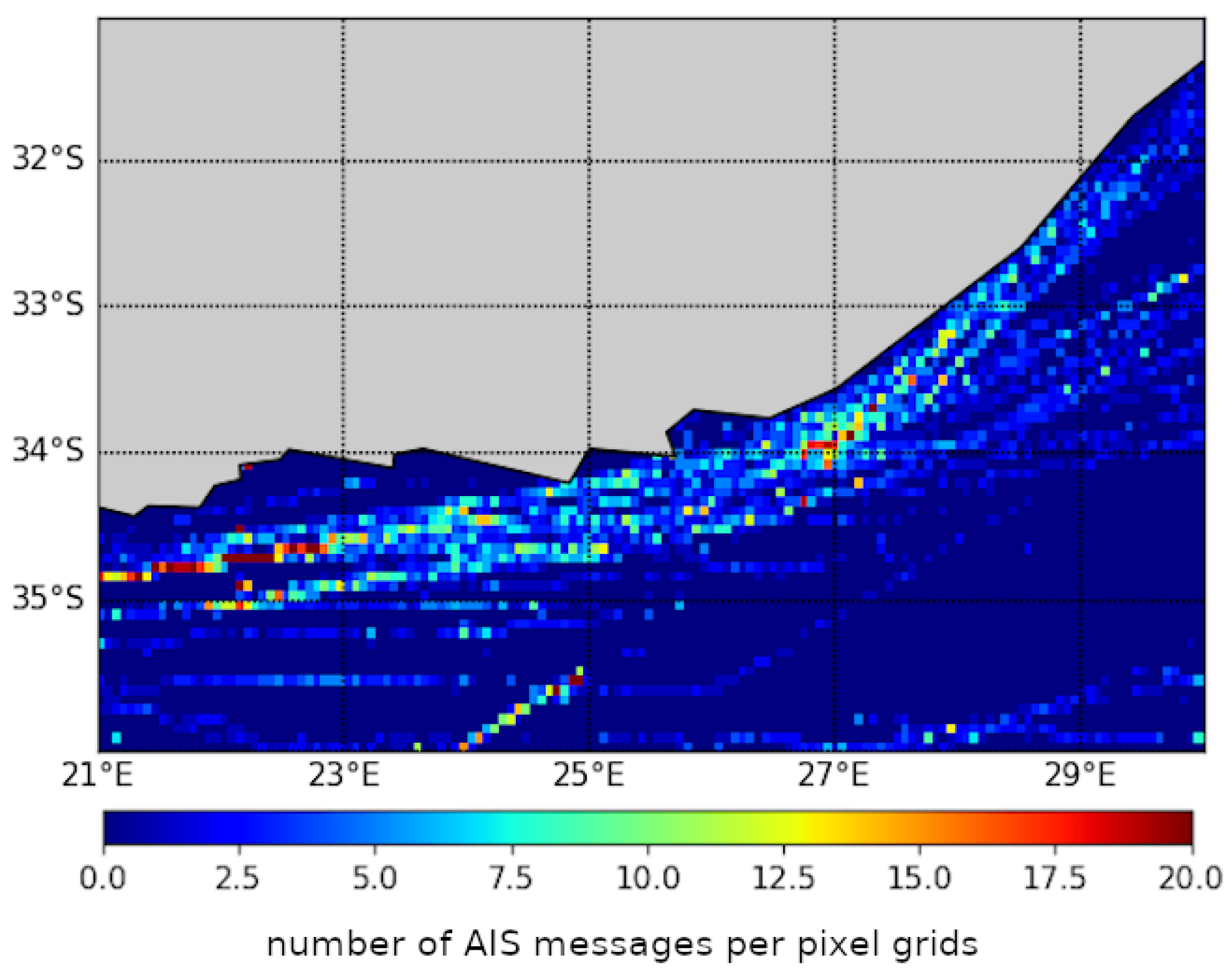
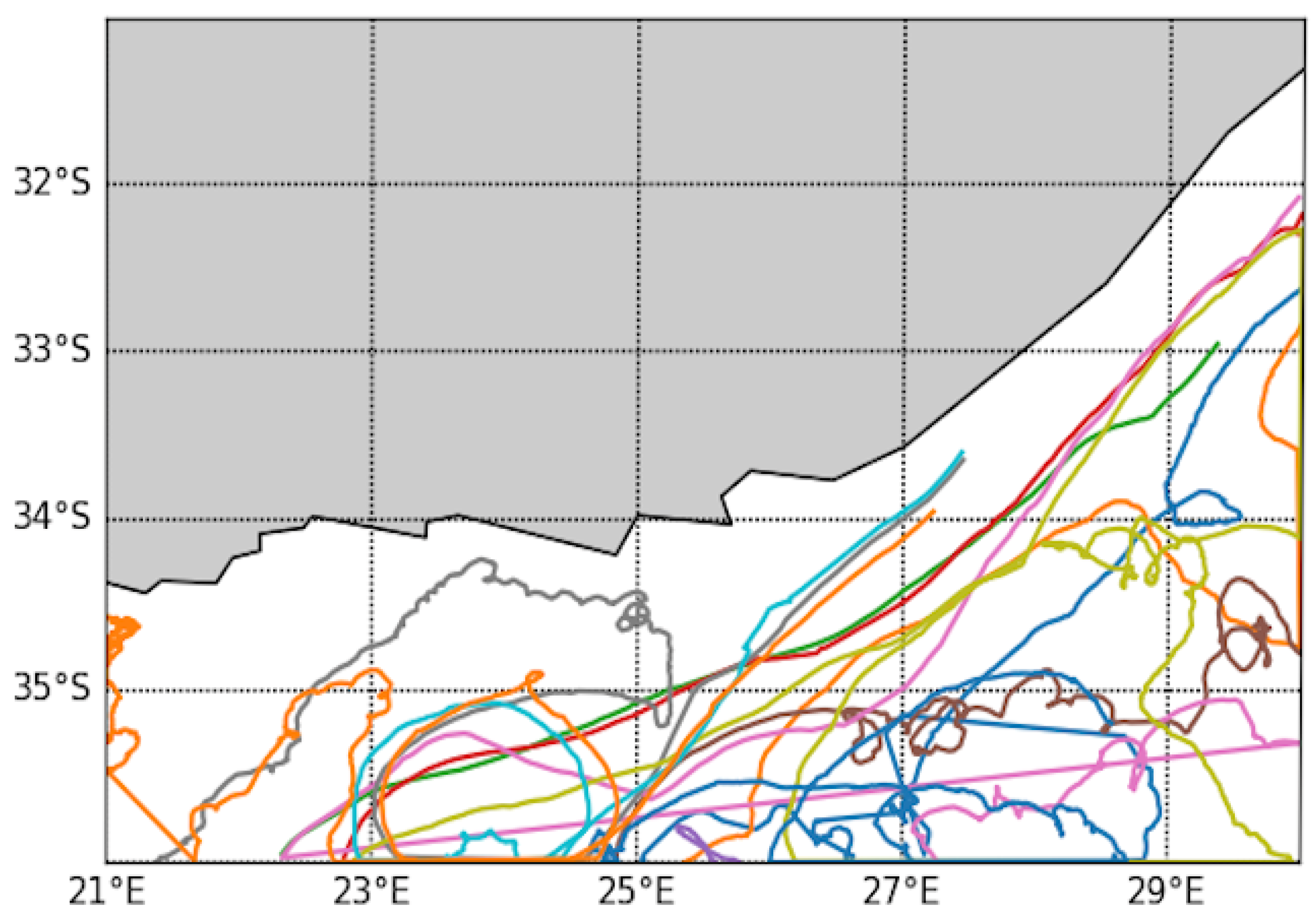
- Numerical experiments for a real dataset demonstrate the relevance of the proposed approach with respect to state-of-the-art approaches. As case-study region, we focus on the Aghulas current off South Africa. This region involves challenging and complex sea surface dynamics for altimetry products. We report significant improvements up to 40% w.r.t. state-of-the-art altimetry-derived assimilation-based products [8,9].
2. Problem Statement and Related Work
2.1. Related Work
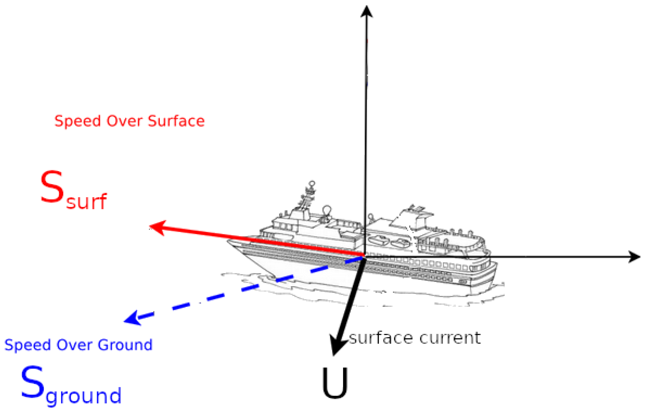
2.2. Observational Model
2.3. Problem Statement
3. Proposed Approach
- Y the available set of AIS messages over a time period ;
- U the spatio-temporal sea surface current field we aim to reconstruct;
- V an external dataset of sea surface current fields that we consider realistic such as reanalysis product or numerical simulations.
3.1. Observation Term J
3.2. Space–Time Dynamical Prior
3.3. Trainable Regulatization Terms
3.4. Training and Evaluation Phase
4. Application to a Real AIS Dataset
4.1. Experimental Setting
- a summer period from 1 January to 20 March;
- a transition period from 9 April to 28 June;
- a winter period from 29 June to 16 September.
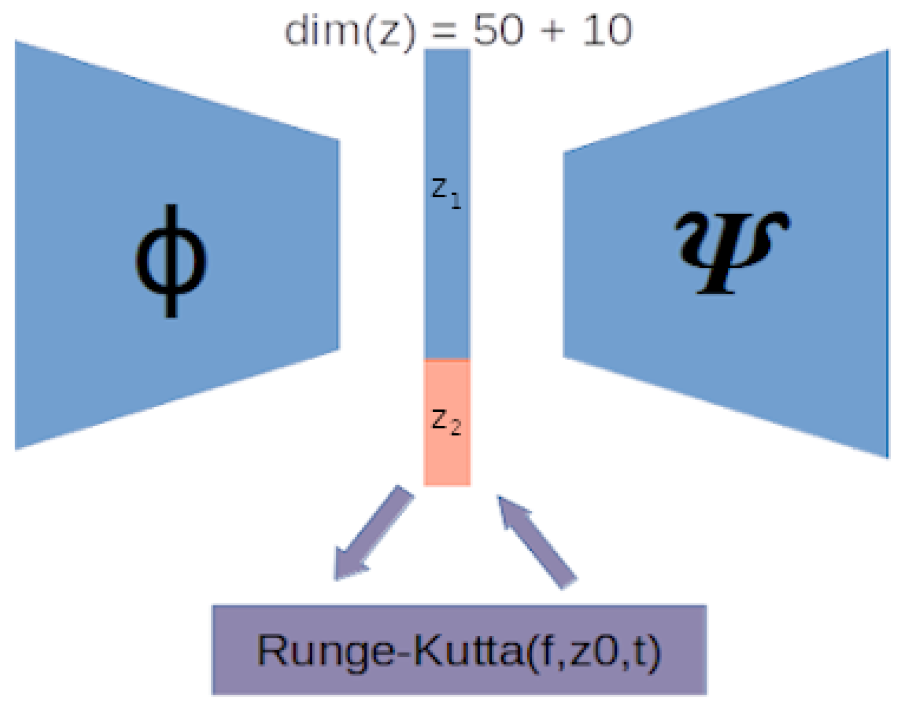
4.2. Neural Network Architecture
- Encoder applies a succession of four convolution layers with ReLU activations, followed by three dense layers with ReLU activation;
- ODE operator f is parametrized by five dense layers with Soft ReLU activation, which guarantees f to be Lipschitz;
- Decoder exploits only the component of the latent variable Z. It involves a four-layer ConvTranspose network with ReLU activation. The output is stated as where denotes the value of the last ConvTranspose output. For all the experiments, we set .
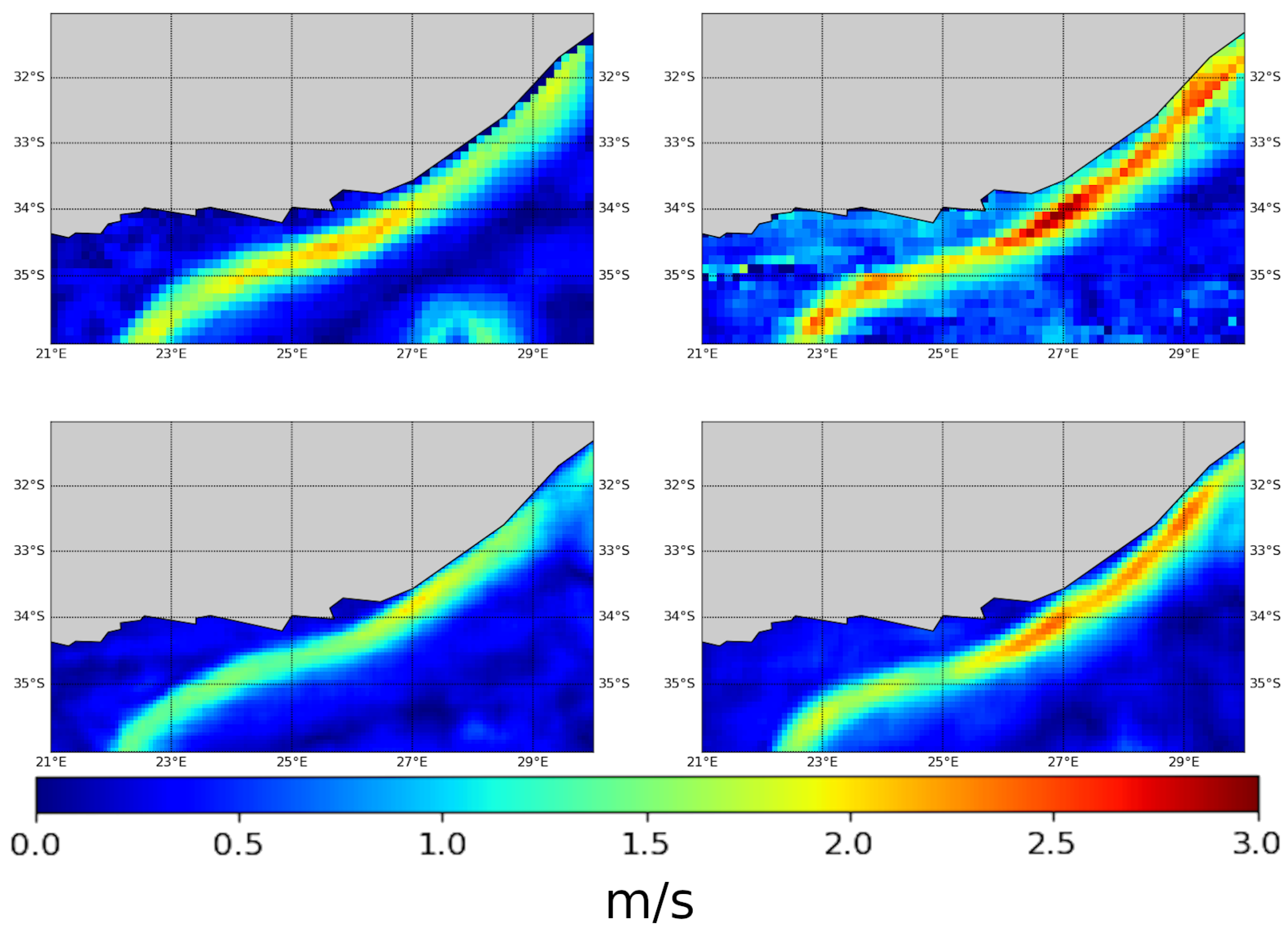
4.3. Results
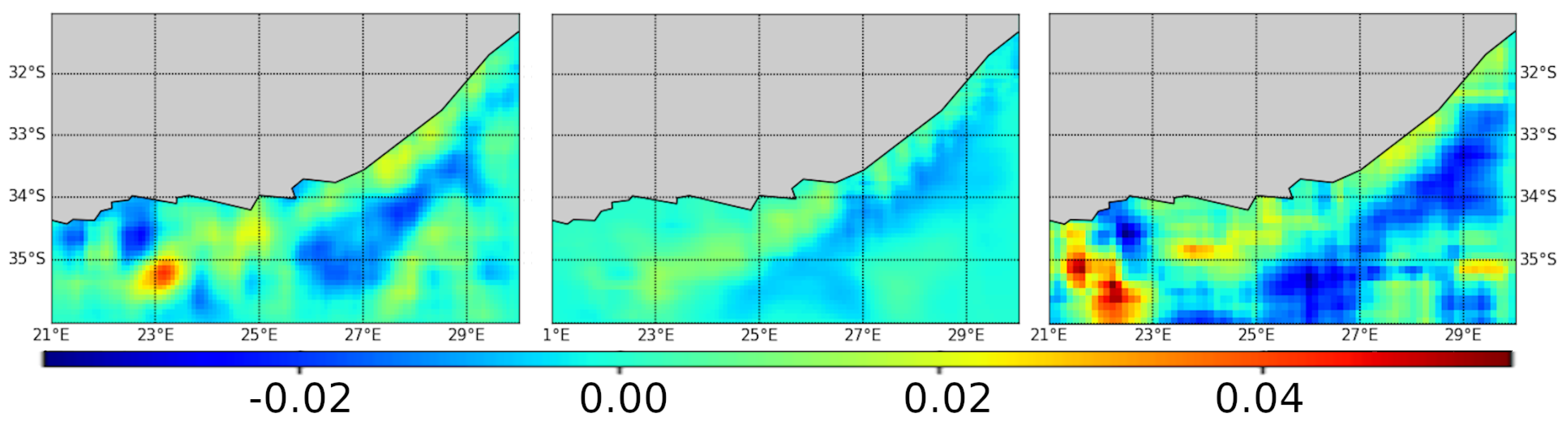
4.4. Ageostrophy
4.5. Generalization Capacity
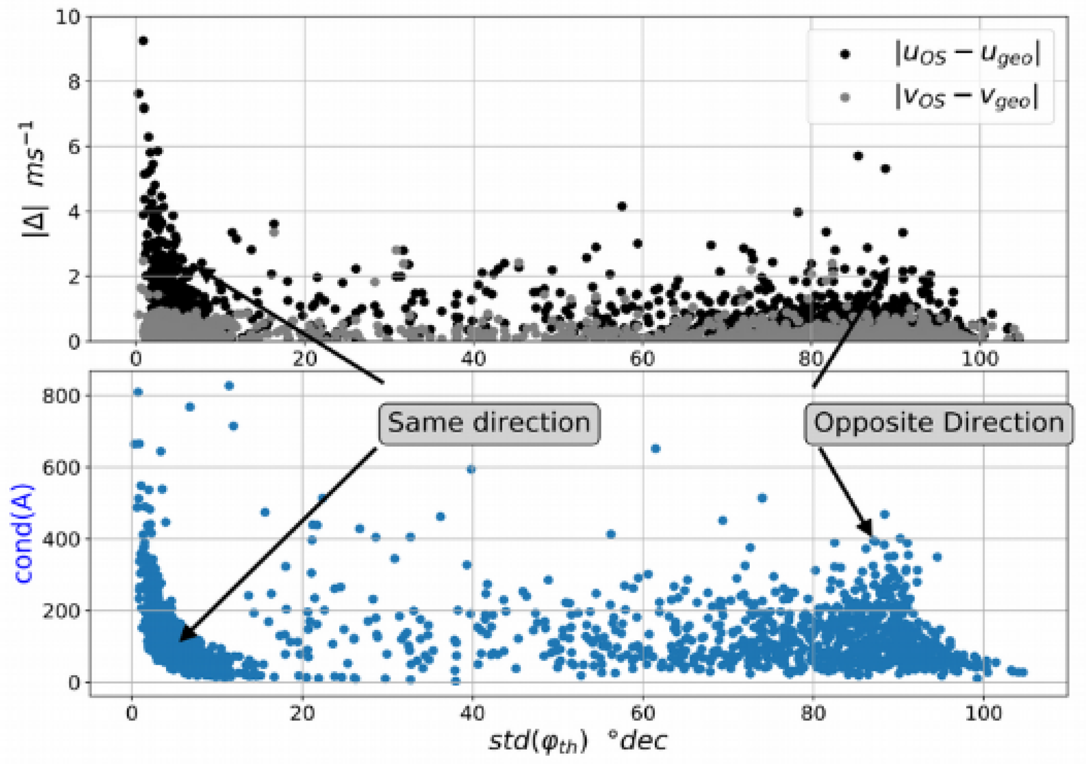
4.6. Sensitivity Analysis
5. Discussion
Author Contributions
Funding
Institutional Review Board Statement
Informed Consent Statement
Data Availability Statement
Acknowledgments
Conflicts of Interest
References
- MarineTraffic—A Day in Numbers. Section: AIS—Essential Knowledge. 2016. Available online: https://www.marinetraffic.com/blog/a-day-in-numbers/ (accessed on 6 May 2021).
- Guichoux, Y.; Lennon, N.T.M. Sea Surface Current Calculation Using Vessel Tracking Datas. In Maritime Knowledge Discovery and Anomaly Detection Workshop; e-Odyn: Plouzané, France, 2015. [Google Scholar]
- Inazu, D.; Ikeya, T.; Waseda, T.; Hibiya, T.; Shigihara, Y. Measuring offshore tsunami currents using ship navigation records. Prog. Earth Planet. Sci. 2018, 5, 38. [Google Scholar] [CrossRef] [Green Version]
- Richardson, P.L.; McKee, T.K. Average Seasonal Variation of the Atlantic Equatorial Currents from Historical Ship Drifts. J. Phys. Oceanogr. 1984, 14, 1226–1238. [Google Scholar] [CrossRef] [Green Version]
- Richardson, P.L.; Reverdin, G. Seasonal cycle of velocity in the Atlantic North Equatorial Countercurrent as measured by surface drifters, current meters, and ship drifts. J. Geophys. Res. 1987, 92, 3691. [Google Scholar] [CrossRef]
- Matthews, J.; Fox, A.; Prandle, D. Radar observation of an along-front jet and transverse flow convergence associated with a North Sea front. Cont. Shelf Res. 1993, 13, 109–130. [Google Scholar] [CrossRef]
- Talagrand, O.; Courtier, P. Variational Assimilation of Meteorological Observations With the Adjoint Vorticity Equation. I: Theory. Q. J. R. Meteorol. Soc. 1987, 113, 1311–1328. [Google Scholar] [CrossRef]
- Taburet, G.; Sanchez-Roman, A.; Ballarotta, M.; Pujol, M.I.; Legeais, F.; Fournier, F.; Faugere, Y.; Dibarboure, G. DUACS DT2018: 25 years of reprocessed sea level altimetry products. Ocean Sci. 2019, 15, 1207–1224. [Google Scholar] [CrossRef] [Green Version]
- Ferry, N.; Parent, L.; Garric, G.; Barnier, B.; Jourdain, N. Mercator Global Eddy Permitting Ocean Reanalysis GLORYS1V1: Description and Results. Mercat.-Ocean Q. Newsl. 2010, 36, 15–27. [Google Scholar]
- Zhang, T.; Zhang, X.; Shi, J.; Wei, S. HyperLi-Net: A hyper-light deep learning network for high-accurate and high-speed ship detection from synthetic aperture radar imagery. ISPRS J. Photogramm. Remote Sens. 2020, 167, 123–153. [Google Scholar] [CrossRef]
- Zhang, T.; Zhang, X.; Ke, X.; Zhan, X.; Shi, J.; Wei, S.; Pan, D.; Li, J.; Su, H.; Zhou, Y.; et al. LS-SSDD-v1.0: A Deep Learning Dataset Dedicated to Small Ship Detection from Large-Scale Sentinel-1 SAR Images. Remote Sens. 2020, 12, 2997. [Google Scholar] [CrossRef]
- Mazzarella, F.; Arguedas, V.F.; Vespe, M. Knowledge-based vessel position prediction using historical AIS data. In Proceedings of the 2015 Sensor Data Fusion: Trends, Solutions, Applications (SDF), Bonn, Germany, 6–8 October 2015; pp. 1–6. [Google Scholar] [CrossRef]
- Nguyen, D.; Vadaine, R.; Hajduch, G.; Garello, R.; Fablet, R. A Multi-task Deep Learning Architecture for Maritime Surveillance using AIS Data Streams. In Proceedings of the 2018 IEEE 5th International Conference on Data Science and Advanced Analytics (DSAA), Turin, Italy, 1–3 October 2018; pp. 331–340. [Google Scholar] [CrossRef] [Green Version]
- Goff, C.L.; Boussidi, B.; Mironov, A.; Guichoux, Y.; Zhen, Y.; Tandeo, P.; Gueguen, S.; Chapron, B. Monitoring the Greater Agulhas Current with AIS Data Information. J. Geophys. Res. Oceans 2021, 126, e2021JC017228. [Google Scholar]
- Carrassi, A.; Bocquet, M.; Bertino, L.; Evensen, G. Data assimilation in the geosciences: An overview of methods, issues, and perspectives. WIREs Clim. Chang. 2018, 9, e535. [Google Scholar] [CrossRef] [Green Version]
- Held, I.M.; Pierrehumbert, R.T.; Garner, S.T.; Swanson, K.L. Surface quasi-geostrophic dynamics. J. Fluid Mech. 1995, 282, 1–20. [Google Scholar] [CrossRef]
- Traon, P.Y.L.; Nadal, F.; Ducet, N. An Improved Mapping Method of Multisatellite Altimeter Data. J. Atmos. Ocean. Technol. 1998, 15, 522–534. [Google Scholar] [CrossRef]
- Cressman, G.P. An operational objective analysis system. Mon. Weather Rev. 1959, 87, 367–374. [Google Scholar] [CrossRef]
- Cressie, N.; Wikle, C. Statistics for Spatio-Temporal Data; John Wiley & Sons: Hoboken, NJ, USA, 2015. [Google Scholar]
- Lindgren, F.; Lindström, J.; Rue, H. An Explicit Link between Gaussian Fields and Gaussian Markov Random Fields: The SPDE Approach; Mathematical Statistics, Centre for Mathematical Sciences, Faculty of Engineering, Lund University: Lund, Sweden, 2010. [Google Scholar]
- Lguensat, R.; Tandeo, P.; Ailliot, P.; Pulido, M.; Fablet, R. The Analog Data Assimilation. Mon. Weather Rev. 2017, 145, 4093–4107. [Google Scholar] [CrossRef] [Green Version]
- Fablet, R.; Drumetz, L.; Rousseau, F. Joint learning of variational representations and solvers for inverse problems with partially-observed data. arXiv 2020, arXiv:2006.03653. [Google Scholar]
- Beckers, J.M.; Rixen, M. EOF Calculations and Data Filling from Incomplete Oceanographic Datasets. J. Atmos. Ocean. Technol. 2003, 20, 1839–1856. [Google Scholar] [CrossRef]
- Fablet, R.; Chapron, B.; Drumetz, L.; Memin, E.; Pannekoucke, O.; Rousseau, F. Learning Variational Data Assimilation Models and Solvers. arXiv 2020, arXiv:2007.12941. [Google Scholar]
- Kobler, E.; Effland, A.; Kunisch, K.; Pock, T. Total Deep Variation for Linear Inverse Problems. arXiv 2020, arXiv:2001.05005. [Google Scholar]
- Kontopoulos, I.; Spiliopoulos, G.; Zissis, D.; Chatzikokolakis, K.; Artikis, A. Countering Real-Time Stream Poisoning: An Architecture for Detecting Vessel Spoofing in Streams of AIS Data. In Proceedings of the 2018 IEEE 16th Intl Conf on Dependable, Autonomic and Secure Computing, 16th Intl Conf on Pervasive Intelligence and Computing, 4th Intl Conf on Big Data Intelligence and Computing and Cyber Science and Technology, Athens, Greece, 12–15 August 2018; pp. 981–986. [Google Scholar] [CrossRef]
- Tran, L.; Yin, X.; Liu, X. Disentangled Representation Learning GAN for Pose-Invariant Face Recognition. In Proceedings of the 2017 IEEE Conference on Computer Vision and Pattern Recognition (CVPR), Honolulu, HI, USA, 21–26 July 2017; pp. 1283–1292. [Google Scholar] [CrossRef]
- Ouala, S.; Nguyen, D.; Drumetz, L.; Chapron, B.; Pascual, A.; Collard, F.; Gaultier, L.; Fablet, R. Learning Latent Dynamics for Partially-Observed Chaotic Systems. arXiv 2019, arXiv:1907.02452. [Google Scholar] [CrossRef] [PubMed]
- Chen, R.T.Q.; Rubanova, Y.; Bettencourt, J.; Duvenaud, D. Neural Ordinary Differential Equations. arXiv 2019, arXiv:1806.07366. [Google Scholar]
- Fablet, R.; Ouala, S.; Herzet, C. Bilinear residual Neural Network for the identification and forecasting of dynamical systems. In Proceedings of the 2018 26th European Signal Processing Conference (EUSIPCO), Rome, Italy, 3–7 September 2018; pp. 1–5. [Google Scholar]
- LeCun, Y.; Bengio, Y.; Hinton, G. Deep learning. Nature 2015, 521, 436–444. [Google Scholar] [CrossRef]
- Kingma, D.P.; Welling, M. Auto-Encoding Variational Bayes. arXiv 2014, arXiv:1312.6114. [Google Scholar]
- Angles, T.; Mallat, S. Generative networks as inverse problems with Scattering transforms. arXiv 2018, arXiv:1805.06621. [Google Scholar]
- Backeberg, B.C.; Johannessen, J.A.; Bertino, L.; Reason, C. The greater Agulhas Current system: An integrated study of its mesoscale variability. J. Oper. Oceanogr. 2008, 1, 29–44. [Google Scholar] [CrossRef] [Green Version]
- Sudre, J.; Maes, C.; Garcon, V. On the global estimates of geostrophic and Ekman surface currents. Limnol. Oceanogr. Fluids Environ. 2013, 3, 1–20. [Google Scholar] [CrossRef] [Green Version]
- Lutjeharms, J.; Cooper, J.; Roberts, M. Upwelling at the inshore edge of the Agulhas Current. Cont. Shelf Res. 2000, 20, 737–761. [Google Scholar] [CrossRef]
- Cao, Y.; Zhu, J.; Navon, I.M.; Luo, Z. A reduced-order approach to four-dimensional variational data assimilation using proper orthogonal decomposition. Int. J. Numer. Methods Fluids 2007, 53, 1571–1583. [Google Scholar] [CrossRef]


| Data | Method | Summer (MSE) | Autumn (MSE) | Winter (MSE) |
|---|---|---|---|---|
| SLA | AVISO | 0.1154 | 0.0802 | 0.0377 |
| SLA +SST | GLORYS | 0.0687 | 0.0816 | 0.0422 |
| AIS | OI | 0.0855 | 0.1330 | 0.1885 |
| AIS | VAE-NODE | 0.1401 | 0.1458 | 0.1563 |
| AIS + OI | VAE-NODE | 0.4001 | 0.1809 | 0.2176 |
| AIS + AVISO | VAE-NODE | 0.1469 | 0.1222 | 0.1127 |
| AIS + GLORYS | VAE-NODE | 0.0498 | 0.0738 | 0.0378 |
| Method | Summer (MSE) | Autumn (MSE) | Winter (MSE) |
|---|---|---|---|
| summer | 0.0498 | 0.1104 | 0.0760 |
| autumn | 0.1101 | 0.0738 | 0.0367 |
| winter | 0.1275 | 0.1210 | 0.0378 |
| Latent Space Dim | MSE |
|---|---|
| 50 + 0 | 0.0779 |
| 50 + 10 | 0.0498 |
| 50 + 20 | 0.0491 |
| 50 + 50 | 0.0620 |
| 10 + 10 | 0.0805 |
| 250 + 10 | 0.0621 |
| T | MSE |
|---|---|
| 4 days | 0.0625 |
| 8 days | 0.0498 |
| 16 days | 0.1231 |
Publisher’s Note: MDPI stays neutral with regard to jurisdictional claims in published maps and institutional affiliations. |
© 2021 by the authors. Licensee MDPI, Basel, Switzerland. This article is an open access article distributed under the terms and conditions of the Creative Commons Attribution (CC BY) license (https://creativecommons.org/licenses/by/4.0/).
Share and Cite
Benaïchouche, S.; Legoff, C.; Guichoux, Y.; Rousseau, F.; Fablet, R. Unsupervised Reconstruction of Sea Surface Currents from AIS Maritime Traffic Data Using Trainable Variational Models. Remote Sens. 2021, 13, 3162. https://0-doi-org.brum.beds.ac.uk/10.3390/rs13163162
Benaïchouche S, Legoff C, Guichoux Y, Rousseau F, Fablet R. Unsupervised Reconstruction of Sea Surface Currents from AIS Maritime Traffic Data Using Trainable Variational Models. Remote Sensing. 2021; 13(16):3162. https://0-doi-org.brum.beds.ac.uk/10.3390/rs13163162
Chicago/Turabian StyleBenaïchouche, Simon, Clément Legoff, Yann Guichoux, François Rousseau, and Ronan Fablet. 2021. "Unsupervised Reconstruction of Sea Surface Currents from AIS Maritime Traffic Data Using Trainable Variational Models" Remote Sensing 13, no. 16: 3162. https://0-doi-org.brum.beds.ac.uk/10.3390/rs13163162