Rice Yield Estimation Based on Vegetation Index and Florescence Spectral Information from UAV Hyperspectral Remote Sensing

Abstract

Rice floret number per unit area as one of the key yield structure parameters is directly related to the final yield of rice. Previous studies paid little attention to the effect of the variations in vegetation indices (VIs) caused by rice flowering on rice yield estimation. Unmanned aerial vehicles (UAV) equipped with hyperspectral cameras can provide high spatial and temporal resolution remote sensing data about the rice canopy, providing possibilities for flowering monitoring. In this study, two consecutive years of rice field experiments were conducted to explore the performance of florescence spectral information in improving the accuracy of VIs-based models for yield estimates. First, the florescence ratio reflectance and florescence difference reflectance, as well as their first derivative reflectance, were defined and then their correlations with rice yield were evaluated. It was found that the florescence spectral information at the seventh day of rice flowering showed the highest correlation with the yield. The sensitive bands to yield were centered at 590 nm, 690 nm and 736 nm–748 nm, 760 nm–768 nm for the first derivative florescence difference reflectance, and 704 nm–760 nm for the first derivative florescence ratio reflectance. The florescence ratio index (FRI) and florescence difference index (FDI) were developed and their abilities to improve the estimation accuracy of models basing on vegetation indices at single-, two- and three-growth stages were tested. With the introduction of florescence spectral information, the single-growth VI-based model produced the most obvious improvement in estimation accuracy, with the coefficient of determination (R²) increasing from 0.748 to 0.799, and the mean absolute percentage error (MAPE) and the root mean squared error (RMSE) decreasing by 11.8% and 10.7%, respectively. Optimized by flowering information, the two-growth stage VIs-based model gave the best performance (R² = 0.869, MAPE = 3.98%, RMSE = 396.02 kg/ha). These results showed that introducing florescence spectral information at the flowering stage into conventional VIs-based yield estimation models is helpful in improving rice yield estimation accuracy. The usefulness of florescence spectral information for yield estimation provides a new idea for the further development and improvement of the crop yield estimation method.

1. Introduction

Timely monitoring of agricultural production and accurate prediction of crop yield are crucial due to the severe economic and social consequences of food shortages [1,2]. Especially, agricultural products have to be increased by 70% by 2050, when the world population is expected to reach 9 billion people [3]. Rice (Oryza sativa L.) is one of the main food crops and the primary staple food for about half the people of the world [4]. The production is related to the national economy and people’s livelihoods, so timely and non-destructive assessments of rice yield information is of great significance to the development of grain procurement, storage, allocation, and foreign trade [5]. Since remote sensing technology has the advantages of a large-area and dynamic monitoring, it is widely used for regional and global crop yield estimation, including rice [6,7,8].

There are three types of crop yield estimation methods based on remote sensing data; (1) common empirical models based on vegetation indices (VIs) [9,10,11,12,13], (2) crop yield estimation by mechanistic models combined with remote sensing data [14,15,16,17,18], and (3) semi-empirical production estimation models based on Gross Primary Production (GPP) or Net primary production (NPP) [19,20]. Among them, empirical models based on VIs are the most widely used method for crop yield estimation due to their simplicity and ease of use [21,22]. This method generally uses the vegetation index at a single growth stage or the combined vegetation indices from multiple growth stages to build univariate or multivariate models for yield estimation [23]. For those statistical rice yield estimation models that are constructed by spectral indices from multiple growth stages such as the tillering stage, jointing stage, booting stage, heading stage, filling stage and maturity stage [24], spectral information at the flowering stage is rarely used, because vegetation indices directly developed by spectral information at the flowering stage is interfered with by white florets, which may result in the error for yield estimates.

However, the spectrum at the flowering stage contains the information of rice floret number per unit area, which is the most important factor relating to yield [25,26,27,28], making the spectral information at the flowering stage crucial for rice yield estimation. To date, the spectral features at the flowering stage has not been considered in rice yield estimation, although some researchers have observed that the presence of flowers can cause canopy spectral changes in certain bands [29,30]. At present, research on remote sensing monitoring of flowering can be categorized into three types: (1) the extraction of floret amount information (flower coverage ratio and flower number) basing on remote sensing data. Thorpa et al. [31] estimated the floret number of leskelaole rape by flower coverage proportion. Carl et al. [32] extracted the proportion of flower area and estimated the florets amount of acacia using unmanned aerial vehicle (UAVs) images. (2) The effects of flowering information on estimation of such vegetation parameters as biomass, coverage and LAI. Shen et al. [33] found that it was difficult to estimate biomass using NDVI and EVI that contain flowering information, but they could estimate biomass more accurately after the removal of flowering information. Fang et al. [34] tested the effects of flowering information on the estimation of rape vegetation coverage at the flowering stage, and proposed a florescence index to improve estimation accuracy. (3) The application of remote sensing-based flowering information. As flowering spectral information is varied with plant types and fruits, it can be used to classify vegetation types [35] or to extract information related to fruits or yield [36].

Since the green part of rice canopy structure is becoming stable at the flowering stage, the ongoing flowering can be regarded as a process in which white florets information is gradually added into the green background. If the canopy spectrum before flowering and the spectral information during flowering could be obtained, it is possible to use the difference of spectral characteristics before and after flowering to optimize the estimation model and improve the accuracy of yield estimation.

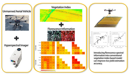
Monitoring spectral changes during the flowering stage requires remote sensing data with high temporal and spatial resolution, which is difficult to meet by current satellite data. Unmanned Aerial Vehicles (UAV) are capable of obtaining the required data as demanded. In this study, UAV equipped with hyperspectral imaging sensors are used to obtain hyperspectral images that cover the whole flowering stage of rice, and new florescence spectral indices were proposed based on spectral characteristics before and after flowering, and then the capabilities of these florescence spectral indices in improving the performance of VIs-based yield estimation models were tested. The objectives of this study were: (1) to determine the characteristic date of the flowering stage and sensitive bands for rice yield estimates by analyzing spectral information of the flowering stage; (2) to propose florescence spectral indices that can express spectral changes during the flowering stage; (3) to optimize traditional multi-growth VIs-based estimation models by combining spectral information at the flowering stage and traditional vegetation indices, so as to verify the performance of florescence spectral index in improving the estimation accuracy of rice yield.

2. Materials and Methods

2.1. Study Area

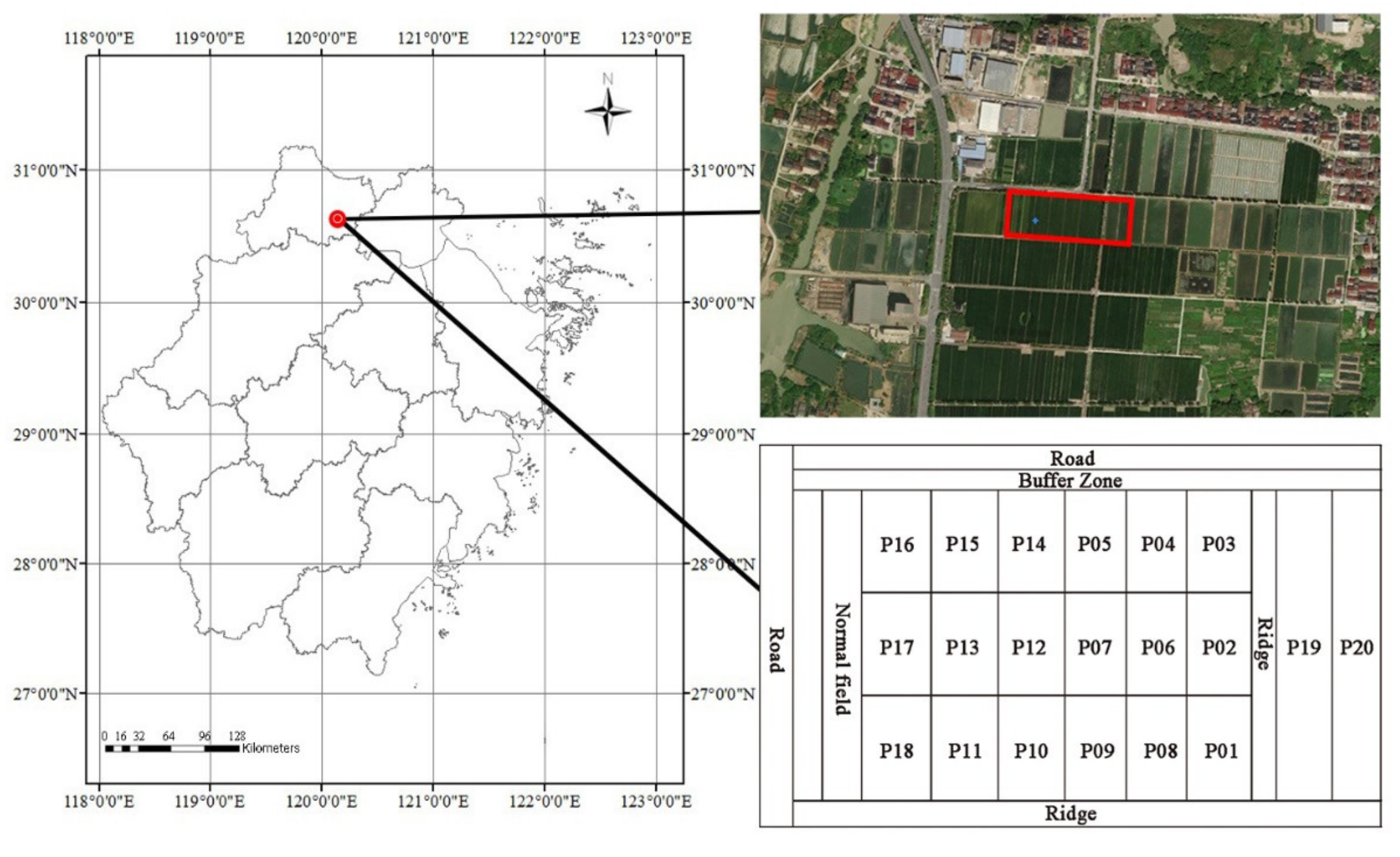
The study area (Figure 1) is located in a grain production functional area of Xiashe Village, Deqing County, Zhejiang Province (120°10′49.34″E, 30°34′21.21″N). It covers about 8200 square meters, with an average annual precipitation of 1379 mm and an average annual temperature of 15 °C. The field experiment was conducted from May to November in 2018 and 2019. Two rice varieties were adopted each year, i.e., Zhejing 99 and Jia 67 in 2018, and Nanjing 9108 and Nanjing 46 in 2019. Five different nitrogen fertilizer levels were set, including N0 (no fertilization), N1 (half of normal fertilization), N2 (normal fertilization), N3 (1.5 times normal fertilization) and N4 (double the normal fertilization), and phosphate and potassium fertilization were consistent with local farming management. The purpose of different nitrogen fertilization levels was not used to analyze the effect of different nitrogen levels on yield, but to increase the variation range of rice yield, so as to make developed models more robust.

The experimental field was set with two varieties, five nitrogen levels and two replicates. Therefore, the experimental field was divided into 20 plots, numbered as P01–P20 (Figure 1).

2.2. Data Collection and Processing

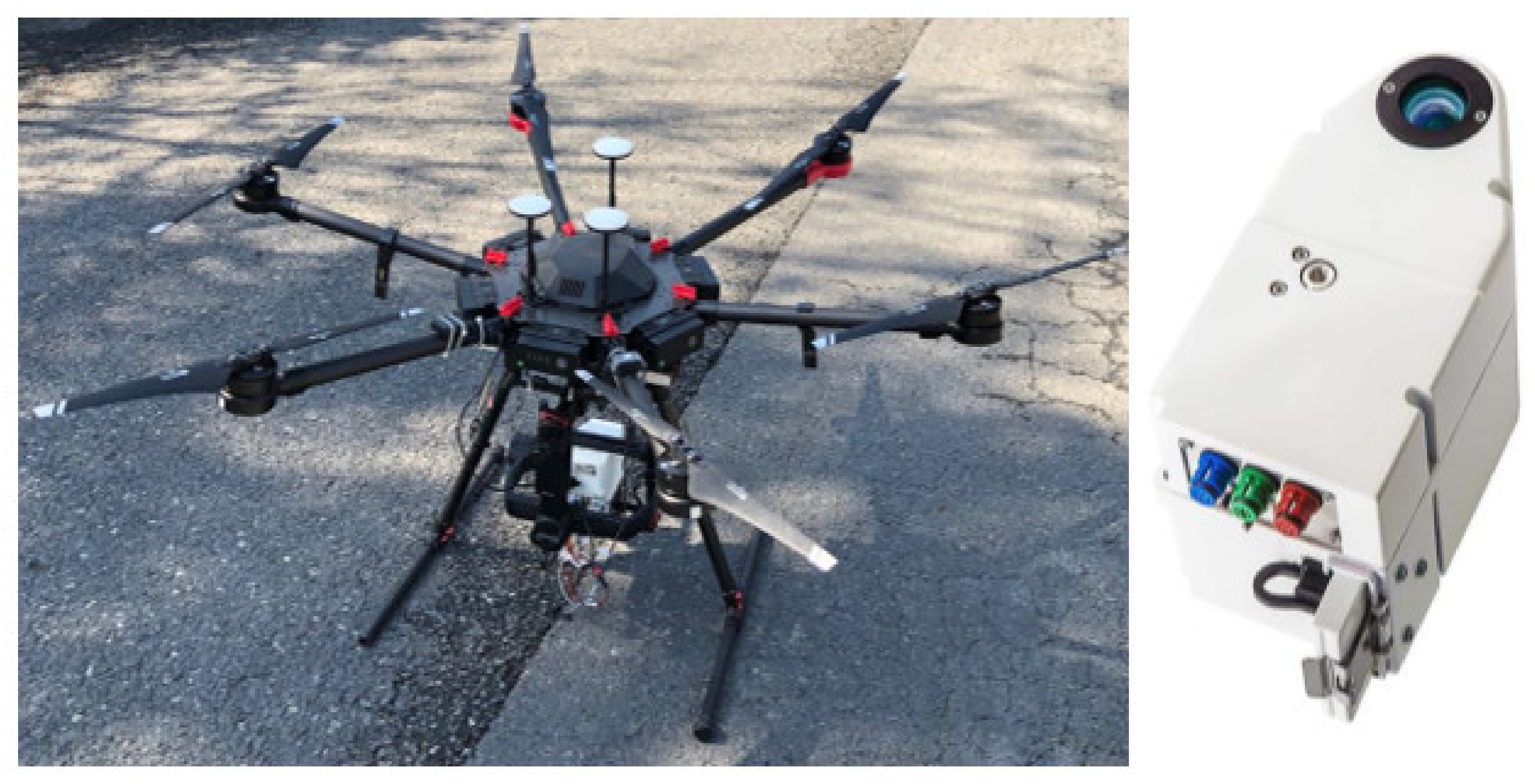
In this study, the DJI M600 Pro UAV equipped with a Rikola hyperspectral imager (Rikola Ltd., Oulu, Finland) (Figure 2) was used to acquire hyperspectral images of rice. The wavelength range of the imager is 500–900 nm, with 62 bands. The imager ’s default band range is 500–900 nm, and the number of bands that can be set is 0–380. In this study, the number of bands was set to 62, and the center wavelength and full width at half maxima of these bands were as shown in

Table 1. Wavelength (WL, nm) and full Width at Half Maxima (FWHM, nm) of all the bands of Rikola.

WL	FWHM	WL	FWHM	WL	FWHM	WL	FWHM	WL	FWHM
504	8.18	592	7.24	680	9.80	733	6.39	816	9.10
512	8.18	596	7.72	685	5.82	736	6.68	824	7.69
520	8.51	600	7.76	688	6.06	740	6.14	832	13.62
528	7.58	604	7.26	692	6.50	744	6.23	840	14.49
536	8.55	608	9.24	696	7.45	748	5.87	848	13.53
544	7.63	616	10.21	700	6.99	752	6.59	856	13.61
552	7.77	624	9.20	704	5.89	760	5.96	864	12.42
560	7.98	632	8.93	709	6.00	768	6.09	872	12.75
568	7.27	635	9.29	712	6.44	776	8.71	880	12.83
576	8.30	650	8.36	716	6.91	784	7.38	888	10.51
580	8.16	656	9.37	720	6.86	792	8.51
584	7.24	664	8.75	724	6.22	800	8.72
588	6.51	672	9.43	728	5.81	808	8.16

Note: green band (WL = 504–560 nm), yellow band (WL = 568–616 nm), red band (WL = 624–680 nm), red-edge band (WL = 685–760 nm), NIR band (WL = 768–888 nm).

[37].

The flight time of UAV was around 11:00 to 12:00 at noon (Beijing local time), when the weather condition was relatively clear and sunny, wind-free and cloud-free. The flight altitude was 200 m, with spatial resolution of hyperspectral image of 13 cm. Hyperspectral images with 1010 by 1010 pixels were obtained at the booting stage, heading stage, filling stage and ripening stage. In order to obtain hyperspectral data before and after flowering, intensive data collection campaigns were carried out from the late booting stage to the end of the flowering stage, with frequency of once every one to two days to ensure the complete time series data before and during the rice flowering stage.

All hyperspectral images were processed with vignetting correction, lens distortion correction, and black level calibration by using the corresponding module functions in a Rikola Hyperspectral Imager V2.1.4 (Rikola Ltd., Oulu, Finland) software to solve the problems of image chromatic aberration, geometric deformation, and temperature-sensing dark current effects. DN values of raw images were transformed to radiance values [38]. Reflectance calculations were carried out using ENVI 5.1 software (Harris Geospatial Solutions, Inc., Boulder, CO, USA) by choosing the gray cloth (diffuse reflection area) in the processing image as the standard reference board and calculating the reflectance of each pixel (Formula (1)), and then obtaining the average reflectance curve of each plot through the Statistics for All ROIs function of ENVI.

$${Ref}_{img}=\frac{Ra{d}_{img}\times Re{f}_{grey}}{Ra{d}_{grey}}$$

(1)

where Rad_grey is the radiation of the reference board, Rad_img is the radiation of image, and Ref_grey is the reflectivity of the reference board.

2.3. Calculation of Vegetation Indices

The normalized vegetation index (NDVI), ratio vegetation index (RVI) and difference vegetation index (DVI) have been widely used in different crops’ growth monitoring [39] and yield estimation [40]. In the study, NDVI, DVI and RVI were calculated using the following equations.

$${NDVI}_{i,j}=\frac{NI{R}_i+RE{D}_j}{NI{R}_i-RE{D}_j}$$

(2)

$${RVI}_{i,j}=\frac{NI{R}_i}{RE{D}_j}$$

(3)

$${DVI}_{i,j}=NI{R}_i-RE{D}_j$$

(4)

where NIR_i is the reflectance of band i in the NIR spectral region (760 nm–900 nm), and RED_j is the reflectance of band j in the red spectral region (620 nm–760 nm).

Since the Rikola hyperspectral camera had 62 bands, it was necessary to determine which band combination was best suitable for yield estimation at different growth stages. Therefore, in this study, all possible two-band combinations between red and near-infrared in types of NDVI, RVI, DVI at four growth stages were calculated. The correlation between these VIs and grain yield were analyzed, and VIs at each growth stages with the highest Pearson correlation coefficient were selected as the optimal vegetation index for rice yield estimation.

2.4. Description of Florescence Spectral Information

2.4.1. Florescence Ratio Reflectance, Difference Reflectance and Their First Derivative Reflectance

The leaves of rice plants grow completely before flowering, making the leaf area index (LAI) basically stable for about two weeks. This means that the green structure of the rice canopy can remain stable during flowering. From the start of flowering, white florets were constantly adding to the unchangeable green background until the full flowering stage, and then diminished till the end of flowering. It could be presumed that the change of canopy reflectance before and after flowering was mainly caused by the change of florets. Therefore, if canopy reflectance before flowering (green background reflectance) and during the flowering stage (florets + green background reflectance) could be obtained, the rice flowering information can be characterized by comparing the difference of canopy reflectance before and after flowering. Based on this mechanism, the idea of florescence ratio reflectance, difference reflectance and their first derivative transformations were proposed in the study. They were expected to enhance the difference in canopy reflectance between before and after flowering. The florescence ratio reflectance (R_{r_Fl(i)}) and florescence difference reflectance (R_{d_Fl(i)}) were calculated as:

$$R_{r\_Fl\left(i\right)}=\frac{R_{Fl\left(i\right)}}{R_{0\_Fl \left(i\right)}}$$

(5)

$$R_{d\_Fl\left(i\right)}=R_{Fl\left(i\right)}-R_{0\_Fl \left(i\right)}$$

(6)

where R_Fl(i) is the canopy spectral reflectance at wavelength i during the flowering stage, and R_{0_Fl(i)} is the canopy spectral reflectance of the exact day before flowering at wavelength i.

Derivative spectral transformation can effectively eliminate the interference of background to target reflectance [41]. Here, the first derivative florescence ratio reflectance (R′_{r_Fl(i)}) and the first derivative florescence difference reflectance (R′_{d_Fl(i)}) were calculated using florescence ratio reflectance and difference reflectance. They were expressed as:

$$R_{r\_Fl\left(i\right)}^{\prime }=\frac{R_{r\_Fl(i+1)}{ -R}_{r\_Fl(i-1)}}{\Delta \gamma }$$

(7)

$$R_{d\_Fl\left(i\right)}^{\prime }=\frac{R_{d\_Fl(i+1)}{ -R}_{d\_Fl(i-1)}}{\Delta \gamma }$$

(8)

where R_{r_Fl(i+1)} and R_{r_Fl(i−1)} are the florescence ratio reflectance at wavelength i + 1 and i − 1. R_{d_Fl(i+1)} and R_{d_Fl(i−1)} are the florescence difference reflectance at wavelength i + 1 and i – 1. Δγ is wavelength difference between wavelength i + 1 and wavelength i − 1.

2.4.2. Formulation of Florescence Indices

Florescence difference index (FDI) and florescence ratio index (FRI) were proposed to enhance the spectral characteristic of florets, while weakening the background signals of the green canopy (

Table 2. Florescence indices tested in this study.

Index	Equation	Index	Equation
FRIa	$\frac{R_{r\_Fl(i)}-R_{r\_Fl(j)}}{R_{r\_Fl(i)}+R_{r\_Fl(j)}}$	FDIa	$\frac{R_{d\_Fl(i)}-R_{d\_Fl(j)}}{R_{d\_Fl(i)}+R_{d\_Fl(j)}}$
FRIb	$\frac{R_{r\_Fl(i)}}{R_{r\_Fl(j)}}$	FDIb	$\frac{R_{d\_Fl(i)}}{R_{d\_Fl(j)}}$
FRIc	$R_{r\_Fl(i)}-R_{r\_Fl(j)}$	FDIc	$R_{d\_Fl(i)}-R_{d\_Fl(j)}$
FRId	$\frac{R_{r\_Fl(i)}^{\prime }-R_{r\_Fl(j)}^{\prime }}{R_{r\_Fl(i)}^{\prime }+R_{r\_Fl(j)}^{\prime }}$	FDId	$\frac{R_{d\_Fl(i)}^{\prime }-R_{d\_Fl(j)}^{\prime }}{R_{d\_Fl(i)}^{\prime }+R_{d\_Fl(j)}^{\prime }}$
FRIe	$\frac{R_{r\_Fl(i)}^{\prime }}{R_{r\_Fl(j)}^{\prime }}$	FDIe	$\frac{R_{d\_Fl(i)}^{\prime }}{R_{d\_Fl(j)}^{\prime }}$
FRIf	$R_{r\_Fl(i)}^{\prime }-R_{r\_Fl(j)}^{\prime }$	FDIf	$R_{d\_Fl(i)}^{\prime }-R_{d\_Fl(j)}^{\prime }$

Note: i and j refers to the specific wavelength of these indices.

).

The aim of constructing the florescence spectral index was to enhance the changes of spectral characteristics caused by rice florets. The spectral transformation methods such as difference, ratio and normalization were used to enhance the spectral contrast, which will help reduce the influence of solar height angle and canopy background when extracting flowering information. Therefore, in this study, florescence ratio reflectance, florescence difference reflectance, first derivative florescence ratio reflectance and first derivative florescence difference reflectance from 500–900 nm of 62 bands were to construct florescence spectral indices in three types of all two-band combinations, and the correlation between these indices and yield were explored. The indices with high correlation coefficients were identified as the optimal florescence spectral indices suitable for yield estimation.

2.5. Model Construction and Evaluation

Multiple linear regression was used to construct rice yield estimation models. Yield was the dependent variable, and spectral information, including all types of vegetation indices, florescence difference or ratio reflectance as well as first derivative florescence reflectance were independent variables.

The parameters adopted to assess the performance of models were the coefficient of determination (R²), average absolute percentage error (MAPE), and root mean square error (RMSE). R² reflected the fitting degree of estimated and measured yield. The higher R² was, the higher the reliability of the yield estimation model was. MAPE and RMSE reflected the error between estimated and measured yield, with lower values indicating higher accuracy. They were defined as:

$${\mathrm{R}}^2=1-\frac{{\displaystyle \sum _i{\left(y-y\prime \right)}^2}}{{\displaystyle \sum _i{\left(y-\overline{y}\right)}^2}}$$

(9)

$$MAPE=\frac{{\displaystyle \sum _{i=1}^n\left|\frac{y-y^{\prime }}{y}\right|}}{n}\times 100\%$$

(10)

$$RMSE=\sqrt{\frac{{\displaystyle \sum _{i=1}^n{\left(y-y^{\prime }\right)}^2}}{\mathrm{n}}}$$

(11)

where y is the measured yield, y′ is the modeled yield, $\overline{y}$ is the average value of the measured yield, and n is the sample size.

The yields in 2018 ranged from 5497.27 to 9494.92kg/ha with their average of 7404.85 kg/ha, while the yields in 2019 ranged from 4413.38 to 8803.24 kg/ha with their average of 7271.62 kg/ha. Due to the differences in rice varieties and fertilization levels in the two years, all samples of two years were ranked by yield from lowest to highest, and were evenly divided into three groups, with 2/3 as the modeling dataset and 1/3 as the validation dataset.

3. Results

3.1. Yield Estimation Basing on VIs

In general, the accuracy of rice yield estimation models increases with a greater number of key growth stages involving in models, but introducing too many growth stages in models will not only make models more complex, but also weaken the interannual robustness of models [38]. Considering that rice spectral information at early growth stages is more easily affected by environmental factors such as water surface and soil background, it is better to estimate rice yield from the booting stage when rice leaves have basically covered the background [42]. Therefore, in this present study, the booting stage and the following three critical growth stages, i.e., the heading, filling, and ripening stages, were tested for yield estimation. The band locations for all selected VIs were shown in

Table 3. Band locations of vegetation indices best suitable for yield estimation.

Sensitive Bands		Booting	Heading	Filling	Ripening
NDVI	band 1	740	733	752	748
	band 2	768	832	880	792
Correlation coefficient		0.872	0.873	0.826	0.663
RVI	band 1	740	748	752	748
	band 2	768	832	880	792
Correlation coefficient		0.871	0.872	0.824	0.662
DVI	band 1	748	748	752	748
	band 2	800	840	864	816
Correlation coefficient		0.817	0.867	0.804	0.681

Note: band 1 is red and band 2 is NIR.

.

As seen, band 1 from all types of vegetation indexes occurred in the red-edge region from 733 nm and 752 nm, but NIR bands were different at different growth stages. For NDVI and RVI at the booting stage, the NIR band was 768 nm; for NDVI at the ripening stage, the NIR band was 792 nm. The NIR bands of the best vegetation indices at other growth stages were located between 800 nm and 880 nm.

3.2. Correlation Analysis between Florescence Ratio Reflectance, Florescence Difference Reflectance and Rice Yield

Taking the data of the P01 plot in 2019 as an example, the florescence difference reflectance and florescence ratio reflectance showed different spectral characteristics, but their variation trends were consistent (Figure 3). Most reflectance of florescence difference reflectance were positive, with the variation ranging from −0.05 to 0.15. The maximum value appeared near 850 nm, and the minimum value occurred near 680 nm. The reflectance of florescence ratio reflectance fluctuated around 1, with most of them greater than 1. The maximum and minimum values appeared around 800 nm and 680 nm, respectively.

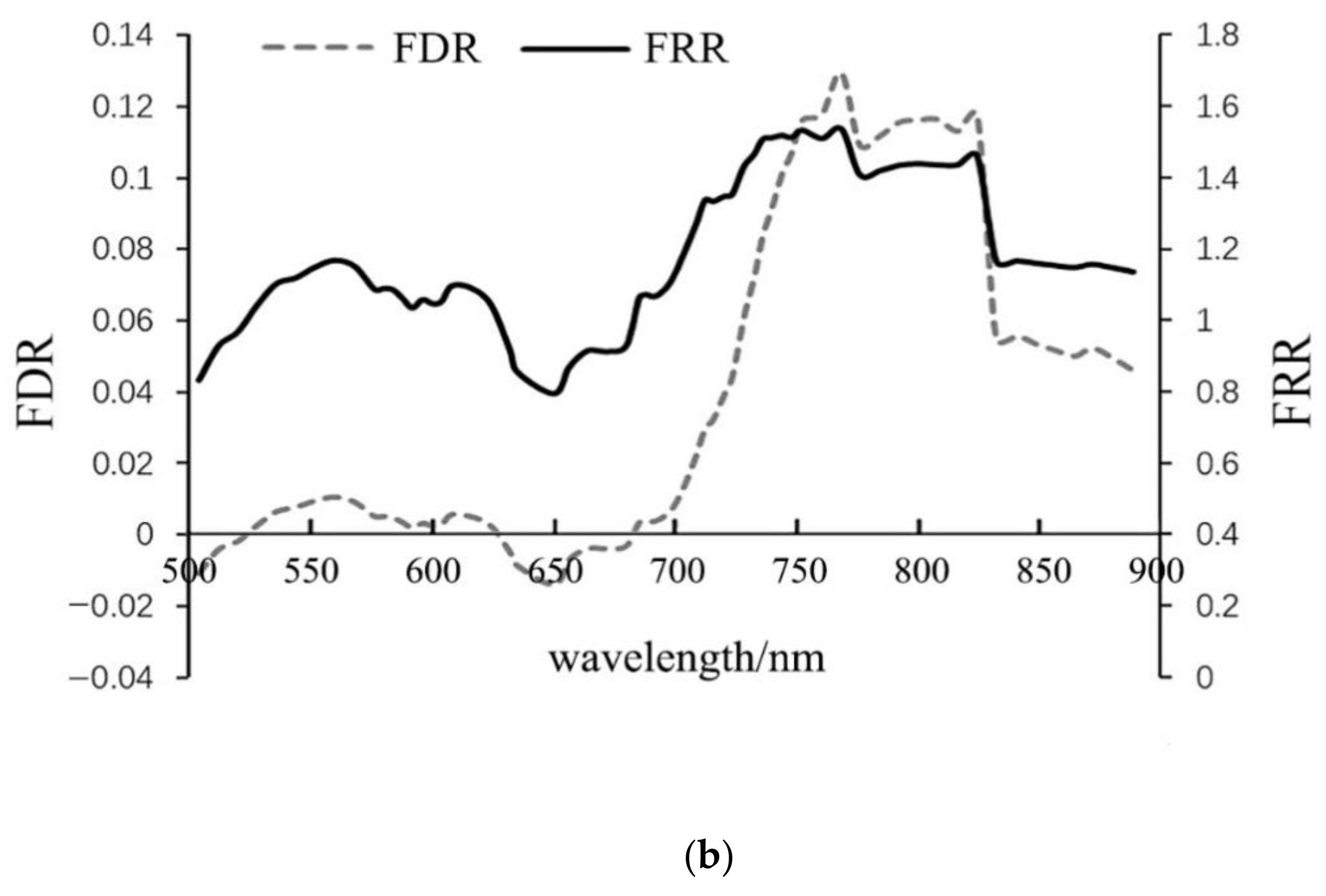
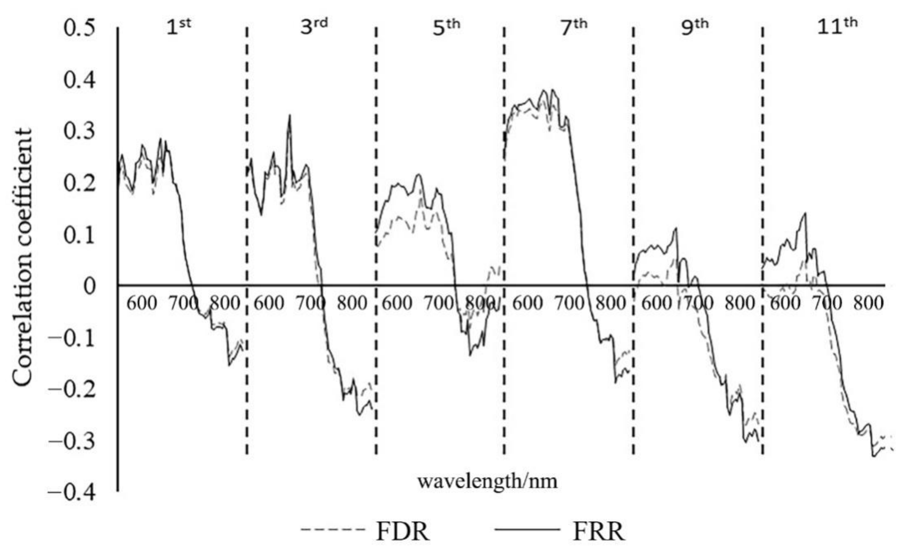
It could be seen that the variation characteristics of the correlation coefficient curved between the florescence ratio reflectance, florescence difference reflectance and yield in the whole flowering stage were basically similar (Figure 4), with the peaks and troughs of the daily correlation coefficient curve highly coincident. The performance of florescence ratio reflectance was better than that of florescence difference reflectance. From the beginning of the flowering stage to the end of the flowering stage, the correlation coefficients increased at first and then decreased, and the best correlationship occurred around the seventh day of the flowering stage, at which showed the biggest correlation coefficient and stable band location. At the early flowering stage, the sensitive bands were mainly concentrated around yellow and red bands of 635 nm and 650 nm, and gradually extended to the red edge spectral region till the full flowering stage, and then completely moved to the near-infrared bands of 830–880 nm at the late stage of flowering.

Since the florescence ratio and difference reflectance at the seventh day of the flowering stage had the highest correlation with the yield, it was considered as the best date for rice yield estimation basing on spectral information at the flowering stage. At the seventh day of the flowering stage, florescence ratio and difference reflectance from 520 nm to 704 nm were best correlated to rice yield, with the biggest correlation coefficient for florescence difference reflectance at 624 nm, and 664 nm for florescence ratio reflectance.

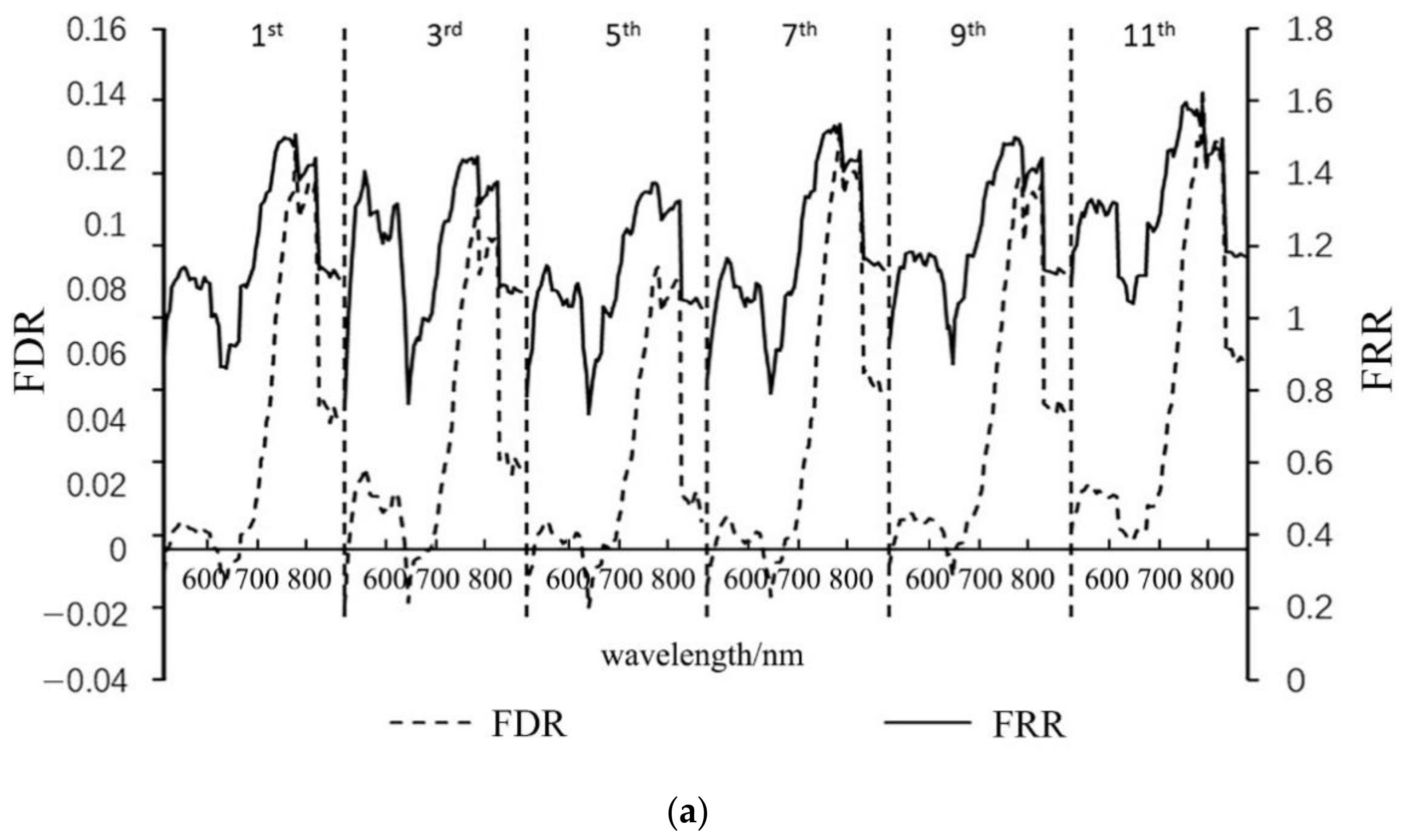
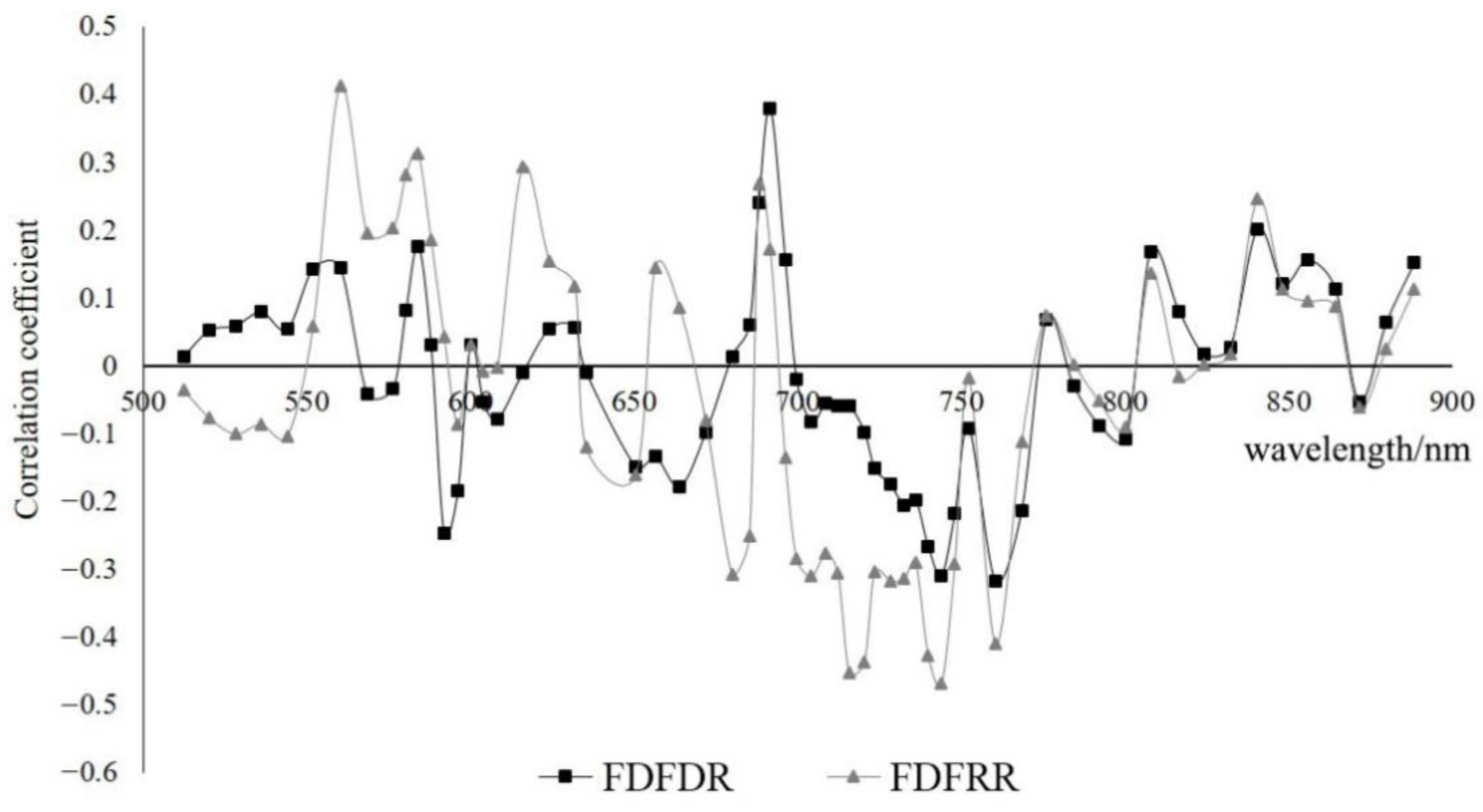
The first derivative ratio reflectance (Figure 5) at 560 nm, 720 nm and 740 nm showed good correlation with yield, and they were 590 nm, 690 nm, 740 nm and 760 nm for the first derivative difference reflectance. Obviously, the first derivative reflectance were better correlated with yield than the difference reflectance or the ratio reflectance.

The results showed that for the first derivative ratio reflectance, the sensitive bands were around green bands 560 nm–568 nm, yellow bands 576 nm–588 nm, red-edge bands 680 nm–760 nm and NIR bands around 840 nm; the highly sensitive bands (top 50% of sensitive bands) were located at 704–760 nm. For the first derivative difference reflectance, sensitive bands were centered at yellow bands 580 nm–596 nm, red bands 664 nm, red-edge bands 688 nm–696 nm, 724 nm–768 nm, and the NIR region 840 nm–864 nm; the highly sensitive bands (top 50% of sensitive bands) were more spread out than the ratio derivative reflectance, mainly centering at 590 nm, 690 nm, 736 nm–748 nm, and 760 nm–768 nm.

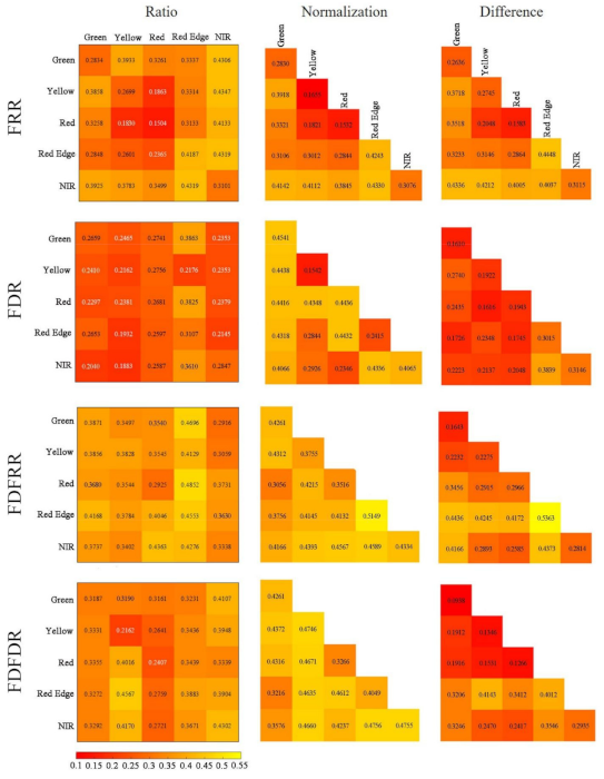
3.3. Development of Florescence Difference Index (FDI) and Florescence Ratio Index (FRI)

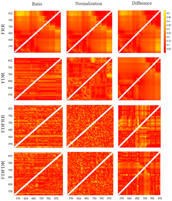
In this study, florescence ratio reflectance, florescence difference reflectance, first derivative florescence ratio reflectance and first derivative florescence difference reflectance from 500–900 nm of 62 bands constructed florescence spectral indices in three types of all two-band combinations, and the correlation between these indices and yield were as in Figure 6. The indices with high correlation coefficients were identified as the florescence spectral indices more suitable for yield estimation.

In general, the first derivative florescence ratio reflectance and the first derivative florescence difference reflectance were better related to yield than the raw florescence ratio and difference reflectance. Additionally, the first derivative florescence ratio reflectance performed better than the first derivative florescence difference reflectance.

For the first derivative florescence ratio reflectance, the types of band combinations with larger correlation coefficients were very diverse, including ratio, normalized and difference combinations: ratio combination of red-edge and red bands, ratio combination of red-edge and green bands, normalized combination of red-edge and red-edge bands, difference combination of red-edge and red-edge bands, difference combination of NIR and red-edge bands. For the first derivative florescence difference reflectance, the larger correlation coefficients were obtained by normalized combinations, including the normalization combinations of NIR and red-edge bands, NIR and NIR bands, NIR and yellow bands, red and yellow bands, and yellow and yellow bands (Figure 7). Compared with the second part of the study, it was found that the denominators in the ratio combination of the first derivative ratio reflectance were always within the sensitive band range, but numerators were not. Most of the bands in the ratio combination and difference combination were within the range of sensitive bands. Additionally, the two bands in a normalization combination of the first derivative difference reflectance basically consisted of a highly sensitive band and a less sensitive (at least generally sensitive) band. The combination of a highly sensitive band and a less sensitive band, such as FRI3 and FRI4, gave the best results. On the basis of band combination analysis, five combinations of the ratio derivative reflectance and of the difference derivative reflectance highly correlated with yield were selected as the florescence difference index (FDI) and florescence ratio index (FRI) for yield estimation. (

Table 4. The expressions of florescence difference index (FDI) and florescence ratio index (FRI) with high correlation with rice yield.

Index	Equation	CC	Index	Equation	CC
FRI1	$\frac{{\rho }_{r\_Fl7th(624)}^{\prime }}{{\rho }_{r\_Fl7th(716)}^{\prime }}$	−0.4852	FDI1	$\frac{{\rho }_{d\_Fl7th(576)}^{\prime }-{\rho }_{d\_Fl7th(664)}^{\prime }}{{\rho }_{d\_Fl7th(576)}^{\prime }+{\rho }_{d\_Fl7th(664)}^{\prime }}$	−0.4671
FRI2	$\frac{{\rho }_{r\_Fl7th(560)}^{\prime }}{{\rho }_{r\_Fl7th(748)}^{\prime }}$	−0.4696	FDI2	$\frac{{\rho }_{d\_Fl7th(596)}^{\prime }-{\rho }_{d\_Fl7th(784)}^{\prime }}{{\rho }_{d\_Fl7th(596)}^{\prime }+{\rho }_{d\_Fl7th(784)}^{\prime }}$	–0.4660
FRI3	$\frac{{\rho }_{r\_Fl7th(696)}^{\prime }-{\rho }_{r\_Fl7th(716)}^{\prime }}{{\rho }_{r\_Fl7th(696)}^{\prime }+{\rho }_{r\_Fl7th(716)}^{\prime }}$	0.5149	FDI3	$\frac{{\rho }_{d\_Fl7th(709)}^{\prime }-{\rho }_{d\_Fl7th(768)}^{\prime }}{{\rho }_{d\_Fl7th(709)}^{\prime }+{\rho }_{d\_Fl7th(768)}^{\prime }}$	0.4756
FRI4	${\rho }_{r\_Fl7th(692)}^{\prime }-{\rho }_{r\_Fl7th(720)}^{\prime }$	0.5363	FDI4	$\frac{{\rho }_{d\_Fl7th(848)}^{\prime }-{\rho }_{d\_Fl7th(872)}^{\prime }}{{\rho }_{d\_Fl7th(848)}^{\prime }+{\rho }_{d\_Fl7th(872)}^{\prime }}$	–0.4755
FRI5	$\frac{{\rho }_{r\_Fl7th(716)}^{\prime }-{\rho }_{r\_Fl7th(800)}^{\prime }}{{\rho }_{r\_Fl7th(716)}^{\prime }+{\rho }_{r\_Fl7th(800)}^{\prime }}$	0.4589	FDI5	$\frac{{\rho }_{d\_Fl7th(576)}^{\prime }-{\rho }_{d\_Fl7th(608)}^{\prime }}{{\rho }_{d\_Fl7th(576)}^{\prime }+{\rho }_{d\_Fl7th(608)}^{\prime }}$	0.4746

Note: CC means coefficient correlation.

).

3.4. Yield Estimation Model

In this study, vegetation indices at different growth stages and florescence spectral indices were used as independent variables, and rice yield was used as the dependent variable. Yield estimation models were established based on both vegetation indices and florescence spectral information. They were compared with the yield estimation models using vegetation indices alone, and the potential of spectral information at the flowering stage in improving yield estimation was analyzed. The yield estimation models are presented in

Table 5. The expressions for the optimization model with single, two and three growth stages involved.

Growth Stage	Model Expression
Single-growth stage	Y = 29882.803 × NDVI(740,768) (Booting)−3.017 × FDI1−78.851 × FDI2-7.921 × FDI4 + 2331.725
Two-growth stage	Y = 24173.141 × NDVI(740,768) (Booting) + 33292.36 × DVI(752,864) (Filling) + 24.836 × FRI1 + 43897.073 × FRI4 + 15.488 × FDI5−32.097
Three-growth stage	Y = 30193.832 × NDVI(740,768) (Booting) − 15773.406 × RVI(748,832) (Heading) + 73832.326 × DVI(752,864) (Filling) + 41129.09 × FRI4−5.211 × FDI4 + 16010.301

:

As seen in

Table 6. Comparisons of the yield estimation models with and without considering florescence spectral information for the modeling dataset.

Growth Stage Combination	Florescence Information	Assessment
		R2	MAPE (%)	RMSE (kg/ha)
Single-growth stage	No	0.748	5.74	548.61
	Yes	0.799	5.06	489.91
Two-growth stage	No	0.833	4.74	446.45
	Yes	0.869	3.98	396.02
Three-growth stage	No	0.838	4.7	439.7
	Yes	0.861	4.33	419.58

, the best single-growth stage model was constructed by NDVI_{(740,768)(Booting)} at the booting stage, with R² of 0.748. The introduction of FDI1(_576,664), FDI2_(596,784) and FDI4_(848,872) into this model effectively improved the model performance, with R² increasing from 0.748 to 0.799, increasing by 6.8%, and MAPE and RMSE decreasing by 11.8% and 10.7%, respectively. For the two-growth stage model, the involved vegetation indices were NDVI_{(740,768) (Booting)} at the booting stage and DVI(_{752,864)(Filling)} at the filling stage. After introducing florescence spectral indices FRI1_(624,716), FRI4_(692,720) and FDI5_{(576, 608)}, the model R² increased by 4.1%, MAPE and RMSE decreased by 16.0% and 11.3%, respectively. For the three-growth stage model, RVI_{(748,832)(Heading)} at the heading stage was added on the basis of the two-growth stage model and the introduction of FRI8_{(692, 720]} and FDI4_(848,872) at the flowering stage increased R² by 2.7%, and decreased MAPE and RMSE by 7.8% and 4.6%, respectively. It could be seen that the performance of estimation models using vegetation indices alone were improved when two or three florescence spectral indices were included. Among the involved florescence spectral indices, FDI4_(848,872) was used in the single-growth stage model and three-growth stage model, and FRI4_(692,720) was introduced in the two-growth stage model and three-growth stage model.

The estimation accuracy of models using vegetation indices alone was improved when more growth stages were involved. With the introduction of florescence spectral indices in these models, estimation accuracy was further improved, especially for the single-growth stage model and two-growth stage model, which showed the most obvious improvements. The obvious increase in estimation accuracy for these two models was partly because of their relatively low accuracy, making them have a greater potential for improvement, while the accuracy of the three-growth stage model was already high and the room for optimization was limited. It could be concluded that spectral information at the flowering stage was very useful in improving the performance of yield estimation models using vegetation indices alone. Taking florets as interference information, weakening the efficiency of spectral information was actually a waste of useful information at the flowering stage.

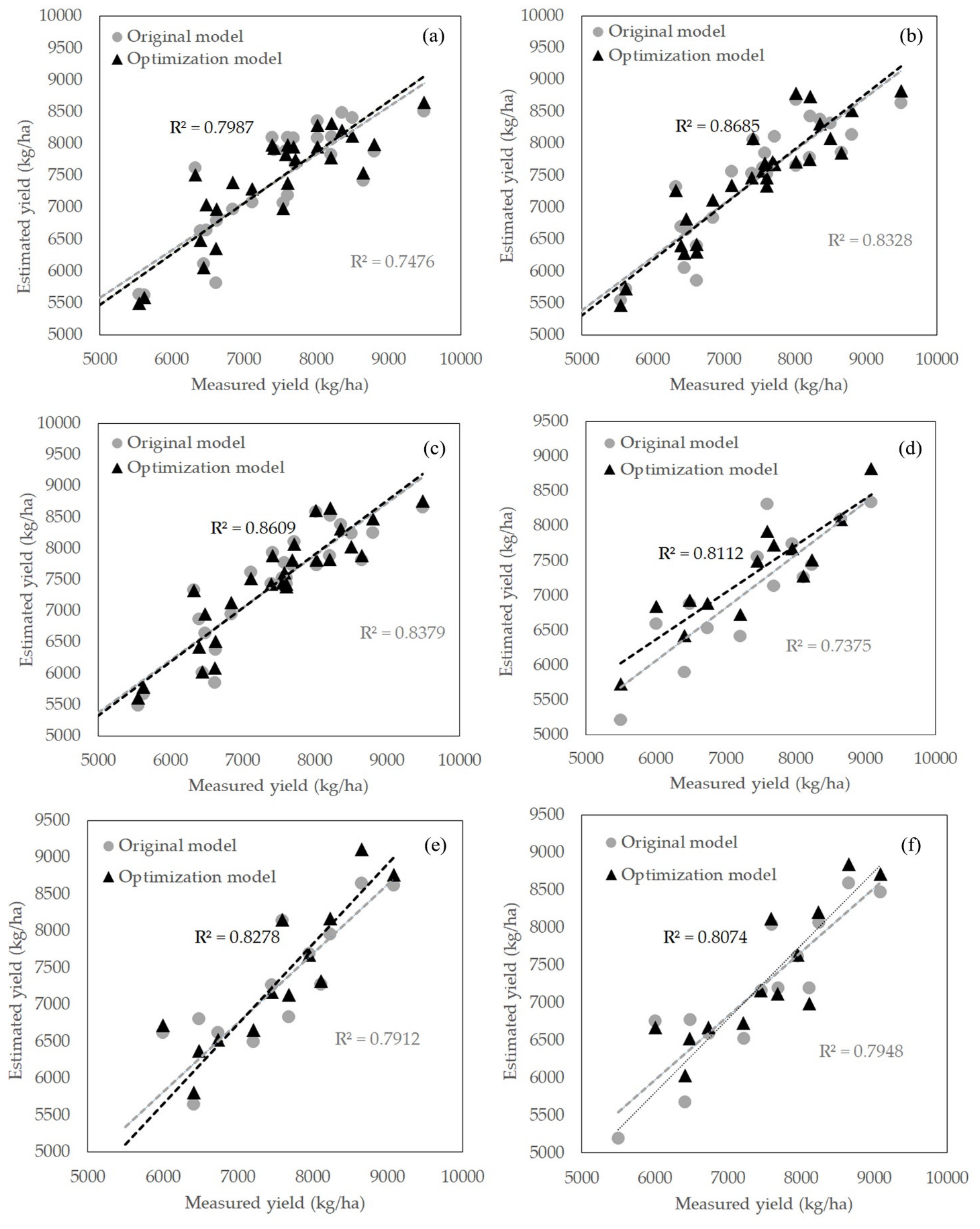
3.5. Validation of Yield Estimation Models

In this section, the established models were evaluated by validation datasets. It was found that the overall test results were similar to these obtained by the calibration dataset, demonstrating the usefulness of florescence spectral information in improving R², MAPE and RMSE of yield estimation models using vegetation indices alone (

Table 7. Comparisons of the yield estimation models with and without considering florescence spectral information for the validation dataset.

Growth Stage Combination	Florescence Information	Assessment
		R2	MAPE (%)	RMSE (kg/ha)
Single-growth stage	No	0.738	7.04	405.92
	Yes	0.811	5.12	328.10
Two-growth stage	No	0.791	6.83	391.68
	Yes	0.828	6.04	376.16
Three-growth stage	No	0.795	6.17	360.54
	Yes	0.807	6.06	373.31

). Moreover, the fitting line of measured and estimated yields of models with flowering information were closer to the 1:1 line (Figure 7). R² of the single-growth stage model, two-growth stage model and three-growth stage model increased by 0.073, 0.037 and 0.012, respectively, with the largest increase obtained by the single growth stage model, whose MAPE and RMSE decreased by 27.3% and 19.2%, respectively.

Additionally, it could be found that yield estimation accuracy of the single-growth stage model based on vegetation index and florescence spectral indices was equivalent to the two-growth stage model using vegetation indices alone, and the same held true for the comparison between the two-growth stage model basing on vegetation indices and florescence spectral information and the three-growth stage model basing on vegetation indices alone. This indicated that the introduction of florescence spectral information into models using spectral indices alone not only helped reduce the number of remote sensing data acquisition, but also realized the accurate rice yield estimation at an earlier time. Compared to the three-growth stage models using vegetation indices alone, the two-growth stage model using vegetation indices and florescence spectral indices was more likely to be a preferred model for rice yield estimation (Figure 8).

4. Discussion

4.1. The Mechanism of Spectral Information at Flowering Stage on Improving Yield Estimation Accuracy

The traditional agronomic methods for rice yield estimation mainly use rice yield components to calculate rice yield per unit area, which is also known as theoretical yield. This theoretical yield has a high correlation with actual yield [43]. Generally, rice yield per unit area can be calculated by the following four yield components [28]:

Yield per unit area = Total grain number per unit area × Seed setting rate × 1000-grain weight

Since the total number of grains per unit area is grossly equal to the number of florets per unit area, the agronomic yield can also be expressed as:

Yield per unit area = Floret number per unit area × Seed setting rate × 1000-grain weight

The contribution rates of these three yield components to yield from high to low are as follows: floret number per unit area > seed setting rate > 1000-grain weight. It can be seen that floret number per unit area plays a major role in the formation of the final yield regardless of types and yield levels of rice. Therefore, the monitoring of the rice canopy at the flowering stage by remote sensing implies the monitoring of florets per unit area, which is the most important component of rice yield. Compared to the traditional empirical models which indirectly estimate rice yield by monitoring rice biomass, leaf area index and other growth parameters [44], this method is essentially a direct monitoring of yield component, that is floret number per unit area. Therefore, introducing spectral information at the flowering stage into traditional VIs-based models can improve the estimation accuracy of rice yields.

However, rice florets are white and small, and it is difficult to obtain pure information about florets. The signals of rice florets received by sensors are weaker than rice canopies, indicating the vulnerability of these signals to environmental factors [45]. Therefore, in our study, the method of constructing florescence difference or ratio reflectance using canopy spectral data at the very day before flowering and these days during the flowering stage are proposed to characterize the florescence spectral information, and further to express the direct monitoring of floret number per unit area.

4.2. Comparisons between This Study and Previous Studies

In this study, the booting stage was shown to be the optimal stage for rice yield estimation with vegetation indices at a single stage. This was because leaf area index reached its maximum at the booting stage. Some studies also found that the booting stage was the most important stage for yield estimation [23,38]. As for the spectral bands for the three types of vegetation indexes, bands in red-edge and near-infrared regions were identified to be the optimal combinations for rice yield estimation. This result was consistent with that of Zhou et al. [23]. Although the effects of rice florets on canopy spectra were seldom studied before, there were a few studies on the effects of rice panicles on rice spectra. For example, He et al. [46] also found that a vegetation index constructed by a combination of red-edge and near-infrared bands could best predict panicles-affected LAI, which proved effectiveness of red-edge and near-infrared bands for monitoring of rice florescence spectral information.

From the aspect of rice yield estimation based on UAV Remote Sensing, Zhou et al. [23] found the best estimation of rice yield was obtained at the booting and heading stages and the corresponding RMSE was 926.46 kg/ha; Wang et al. [47] combined vegetation indices and textural information from UAV hyperspectral images to estimate rice yield, and a RMSE of 521 kg/ha was obtained. In this study, after some florescence spectral indices were introduced, the relatively smaller RMSE values were obtained. For the two-growth stage and three-growth stage models the RMSE values were 376.16 kg/ha and 373.31 kg/ha, respectively. This showed the importance of florescence information in yield estimation.

4.3. Shortcomings of the Study

Since the florets of a panicle bloom from the top first, then to the bottom, with florets at the top opening first, this makes the flowering duration of different panicles not always same. The flowering durations of different rice plants are different even for those in the same field. However, full flowering is generally reached at the seventh day of the flowering stage. Therefore, the seventh day of the flowering stage is likely to be the most suitable date for monitoring florescence spectral information. In this present study, due to the unfavorable weather conditions, the spectral information at the flowering stage was not obtained on a daily basis, making the conclusion that the seventh day of the flowering stage ass the characteristic date questionable. However, it is sure that the characteristic date should be within the sixth to eighth day of the flowering stage. Taking into account that rice flowering is a cumulative process, the future study can try describing rice flowering information in the form of integral or other functions to solve the problem.

5. Conclusions

This study fully used the direct relationship between florescence spectral information and rice yield, analyzed the sensitive spectral bands to rice yield, and optimized multi-stage VIs-based yield estimation models. The following conclusions can be drawn:

(1)

For the first derivative florescence ratio reflectance, the sensitive bands to yield were centered at green bands 560 nm–568 nm, yellow bands 576 nm–588 nm, red-edge bands 680 nm–760 nm and NIR bands around 840 nm; the highly sensitive bands (top 50% of the sensitive bands) were located at 704 nm–760 nm (red-edge). For the first derivative florescence difference reflectance, the sensitive bands were yellow bands 580 nm–596 nm, red bands 664 nm, red-edge bands 688 nm–696 nm, 724 nm–768 nm, the NIR region 840 nm–864 nm, and the highly sensitive bands (top 50% of the sensitive bands) were 590 nm (yellow), 690 nm and 736 nm–748 nm, and 760 nm–768 nm.

(2)

The useful florescence spectral indices, FDI and FRI, were mainly constructed with NIR bands, red-edge bands and yellow bands as denominators and bands from those that closely relate to the yield as numerators.

(3)

The best date for monitoring the spectral information of rice flowering was at around the seventh day of the flowering stage.

(4)

The introduction of florescence information into VIs-based models could not only improve the accuracy of yield estimation, but is also helpful in realizing rice yield estimations at an earlier stage.

In addition, this study was carried out using the data of a two-year experiment with specific rice varieties, so data of more years and about more rice varieties are needed to verify the effectiveness of models proposed in the study. The monitoring of spectral changes at the flowering stage requires remote sensing data with temporal resolution at a day level, which is difficult to be met by satellite data at present. Besides, the proposed method is waiting to be tested using other crop species and other remotely-sensed data. In the future, with the development of high spatial–temporal resolution technology of satellites, this method is expected to realize the application of large-scale yield estimation based on satellite data.