Systematic Approach for Tunnel Deformation Monitoring with Terrestrial Laser Scanning

Abstract

The use of terrestrial laser scanning (TLS) point clouds for tunnel deformation measurement has elicited much interest. However, general methods of point-cloud processing in tunnels are still under investigation, given the high accuracy and efficiency requirements in this area. This study discusses a systematic method of analyzing tunnel deformation. Point clouds from different stations need to be registered rapidly and with high accuracy before point-cloud processing. An orientation method of TLS in tunnels that uses a positioning base made in the laboratory is proposed for fast point-cloud registration. The calibration methods of the positioning base are demonstrated herein. In addition, an improved moving least-squares method is proposed as a way to reconstruct the centerline of a tunnel from unorganized point clouds. Then, the normal planes of the centerline are calculated and are used to serve as the reference plane for point-cloud projection. The convergence of the tunnel cross-section is analyzed, based on each point cloud slice, to determine the safety status of the tunnel. Furthermore, the results of the deformation analysis of a particular shield tunnel site are briefly discussed.

1. Introduction

Tunnel construction has boomed in several metropolises because the inclusion of a tunnel makes traffic movement efficient and convenient. Tunnel deformation after the completion of a tunnel project is one of the major phenomena that affect the safety status of a tunnel under service. It is also the reason for ambient stress changes that also affect the safety state of a tunnel. Therefore, tunnel deformation must be monitored. If the deformation exceeds certain values, which are typically a few centimeters, then the safety condition of the tunnel is comparatively severe. Conventionally, deformation monitoring is mainly conducted based on sparsely sampled points that are surveyed using high-accuracy devices, such as total stations and geodetic theodolites, but these are time-consuming and labor-intensive. With a conventional method, the local deformation state of a tunnel is reflected by the results from the comparison of different time series data using the point-wise method of total stations or georobots at specific locations. The apparent drawbacks of the conventional approach include the following: only the deformation in a very limited set of points can be measured, and obtaining a complete surface model of the tunnel wall is impossible [1]. Therefore, the real structural health status of the tunnel, especially a shield tunnel, cannot be thoroughly reflected using the conventional method, which pays more attention to the convergence deformation of shield segments. Moreover, once a tunnel is in service, the time allowed for deformation monitoring work is limited. Consequently, the detailed and accurate measurement of tunnel elements with conventional instruments is generally unavailable. Another existing tunnel deformation monitoring method is based on photogrammetry theory and integrates a camera with a laser rangefinder [2]. Image-based approaches have a significant impact on the aspects of operational efficiency and cost-saving. However, these approaches are influenced by the lighting environment. In addition, the automatic processing of extensive metadata is difficult to achieve.

The emergence of the terrestrial laser scanning (TLS) technique in recent years has opened up new perspectives on the recording and 3D reconstruction of tunnel walls at various stages of construction [3], particularly the daily monitoring of tunnels. Compared with conventional methods, TLS is a powerful technique that can acquire the spatial data of objects with effectiveness and integrity. The images can also be stored simultaneously during the course of laser scanning. Hence, TLS is the most suitable method for tunnel structure health diagnosis. Many studies have tested the capability of TLS to analyze tunnel deformation, and several developments have been achieved [4,5,6,7,8,9,10]. However, the systematic, theoretical, and extensive aspects of the technique are still under research. As is well known in the field, shield tunnel deformation monitoring has a higher accuracy requirement in terms of segment deformation analysis. Therefore, this study focuses on the aspects of accuracy and efficiency in the course of data collection and processing.

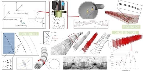
For the critical step of multi-view data registration in tunnels, a fast point cloud registration method is presented in this paper to solve the problem of error propagation. Generally, the iterative closest point (ICP) algorithm is used to register point clouds from different scans. However, when confronted with millions of points, ICP is time-consuming when the initial attitude is unknown. Despite the prevalence of feature-based registration methods in data transformation, whether these approaches can adequately satisfy the accuracy requirement of tunnel deformation analysis remains unclear. The present study aims to develop a systematic method for tunnel deformation monitoring with accurate point-cloud data. According to the procedures shown in Figure 1, the proposed method consists of three main stages. First, an orientation method of TLS (OMTLS) is proposed for point-cloud registration from different scan stations. At this stage, a positioning base (PB) is designed for the precise orientation of the terrestrial laser scanner to the reference coordinate. With the help of the PB, the point clouds from individual scan stations are directly transformed into the reference system without further transformation. Second, the moving least-squares (MLS) method is adopted to thin the scattered point clouds and obtain the centerline of the tunnel from the point clouds. In this process, the point clouds acquired from TLS are projected onto an appropriate plane and then converted to a planar image for data compression and extraction. The centerline is constructed through the MLS method and serves as the normal vector of the reference plane for tunnel cross-section extraction. Lastly, the convergence of the tunnel profile is analyzed, based on each point cloud cross-section, to determine the safety status of the tunnel. In this study, the point clouds may represent a simple, smooth curve without self-intersection, and the research target is mainly the shield tunnel.

The rest of this paper is organized as follows. Section 2 discusses the theoretical background of point cloud processing. Section 2.1 lists related research, Section 2.2 introduces the principle of OMTLS, and Section 2.3 describes the calibration method of the PB. Section 3 introduces the MLS technique and describes several difficulties associated with this approach. Section 3.1 presents an improved version of MLS, Section 3.2 shows the construction of the centerline with a smooth curve, and Section 3.3 discusses tunnel profile generation. Section 4 presents a concrete application of tunnel deformation analysis, that is, the convergence analysis of a tunnel wall. The paper ends with our research conclusions.

2. List of Methods

2.1. Related Work

Point-cloud registration plays an important role in 3D model reconstruction. A popular method of aligning two separate point clouds is the ICP algorithm [11,12]. ICP starts with two point clouds and an estimate of the aligning rigid-body transform. Then, it iteratively refines the transform by alternating between choosing the corresponding points across the point clouds and finding the best rotation and translation that minimize the error metric, based on the distance between the corresponding points [13]. Several improved versions of ICP, such as those in [14,15,16,17,18,19], have been proposed in recent years. However, ICP adopts only a local search algorithm to recover the correspondence between two point clouds and minimizes the sum of square distances between possible corresponding points. It sometimes converges slowly and tends to fall into local minima. Furthermore, tunnels have a tubular shape with extensively scattered point clouds; thus, directly using ICP to register point clouds is time-consuming and easily causes error propagation. In this study, a method based on the PB is proposed to conduct the data registration of tunnels, which aims to cope with the inaccuracy of current registration methods in tunnels. The detailed procedure is discussed in the following section.

Conventional deformation analysis studies are based on displacement data, obtained through geodetic surveying and geotechnical techniques. However, in tunnel deformation monitoring, the change in tunnel lining segment convergence is an important item in structural analysis. Usually, a total station is utilized to obtain the points on the profile for tunnel convergence analysis. However, when data are obtained through the TLS technique, the crucial issue is extracting the centerline from the point clouds to generate the cross-sections for convergence deformation analysis. Thus, curve reconstruction from unorganized point clouds has become a key problem. The MLS method, which uses the local best approximation of scattered point clouds, was first developed by McLain [20,21]. Since then, many improvements have been proposed to develop the algorithm and used it to thin point clouds in terms of efficiency [22,23], rendering [24], stability [25], and other aspects. For instance, Lee [26] presented an algorithm based on MLS to construct the medial axis from point clouds. In his research, the Euclidean minimum spanning tree, region expansion, and refining iteration were used separately to reconstruct a smooth curve. The selection of an appropriate adjustment parameter ($h$) was also discussed using the correlation concept, which is instrumental in the current research. Alexa et al. [27] provided a definition of a smooth manifold surface from a set of points close to the original surface. They divided the MLS projection procedure into three steps and presented an efficient MLS solution. In this paper, a method for centerline generation from point clouds is presented. The improvement provided by MLS for thinning point clouds is discussed in the subsequent section.

2.2. Principle of OMTLS

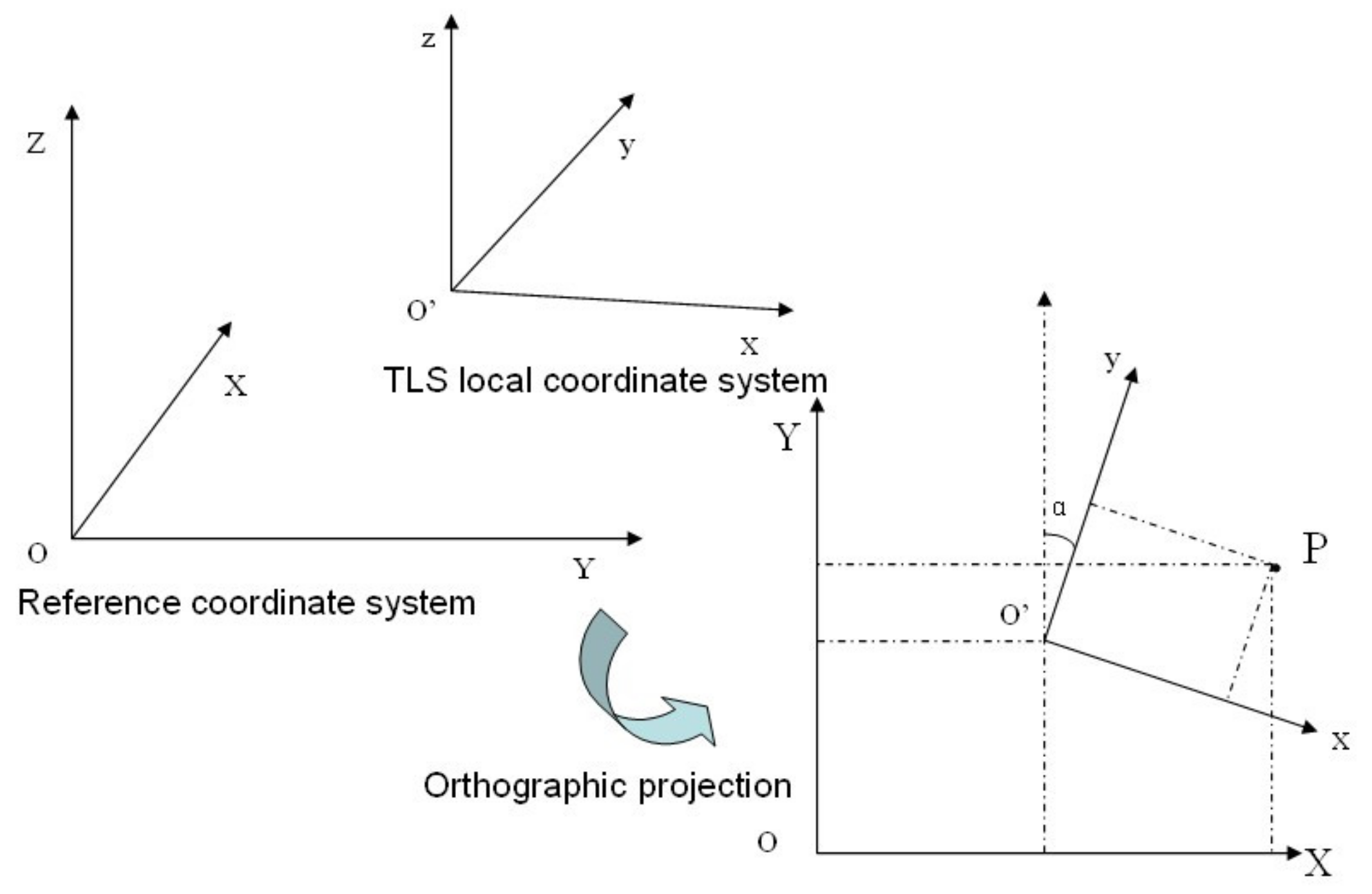
Owing to the technical characteristic of TLS, point clouds acquired from TLS have to be transformed into a common coordinate system to represent the entire object. In practice, conventional methods are prone to error propagation during data registration. Moreover, as the volume of data increases, data registration becomes more and more memory-intensive and time-consuming. Therefore, the critical aspect of tunnel data registration is to improve accuracy and efficiency. For this purpose, OMTLS is proposed as a method to rapidly and precisely transform point clouds into a common reference system. The principle of OMTLS is shown in Figure 2.

In Figure 2, $O-XYZ$ is the reference coordinate system, and $O^{\prime }-xyz$ denotes the TLS local coordinate system. The vertical directions ($Z$) in the two coordinate systems are parallel to each other, after leveling in the tunnel monitoring system. Thus, to transform point clouds in the local system into the reference system, the following two parameters must be determined initially:

(i).

$O^{\prime }$$(X_0,Y_0,Z_0)$, which is the origin of the local system in the reference system;

(ii).

Points $p$$(X_p,Y_p,Z_p)$ and $p^{\prime }$$(x_p,y_p,z_p)$ in the reference and local systems, respectively.

If the two factors mentioned above are known, then the rotation angle $\alpha$ can be computed, based on the following formula:

$$\left\{\begin{array}{l}{X}_p=X_0+x_p\cos \alpha -y_p\sin \alpha \\ Y_p=Y_0+x_p\sin \alpha +y_p\cos \alpha \end{array}\right.$$

(1)

Equation (1) can be rewritten as:

$$\left(\begin{array}{l}{X}_p\\ Y_p\end{array}\right)=\left(\begin{array}{l}{X}_0\\ Y_0\end{array}\right)+\left(\begin{array}{cc}{x}_p& -y_p\\ x_p& y_p\end{array}\right)\left(\begin{array}{l}\cos \alpha \\ \sin \alpha \end{array}\right)$$

(2)

Equation (2) can be expressed as:

$$\left(\begin{array}{l}\cos \alpha \\ \sin \alpha \end{array}\right)=\frac{1}{x_p^2+y_p^2}\left(\begin{array}{c}{x}_p(X_p-X_0)+y_p(Y_p-Y_0)\\ -y_p(X_p-X_0)+x_p(Y_p-Y_0)\end{array}\right)$$

(3)

The rotation angle $\alpha$ is thus defined as:

$$\tan \alpha =\frac{-y_p^{}(X_p-X_0)+x_p^{}(Y_P-Y_0)}{x_p^{}(X_p-X_0)+y_p^{}(Y_P-Y_0)}$$

(4)

Given that the local system is a right-hand system, and the reference system is a left-hand system, a rotation of $\pm {180}^{\circ }$ is required, with the azimuth quadrant being known in advance. Thus, the final rotation angle ($\alpha$) can be obtained using Equation (4). In addition, given rotation angle $\alpha$, the local system can be transformed into the reference system by using Equation (5) directly:

$$\left[\begin{array}{l}{X}_p\\ Y_p\\ Z_p\end{array}\right]=\left[\begin{array}{l}{X}_0\\ Y_0\\ Z_0\end{array}\right]+\left[\begin{array}{ccc}\cos \alpha & -\sin \alpha & 0\\ \sin \alpha & \cos \alpha & 0\\ 0& 0& 1\end{array}\right]\cdot \left[\begin{array}{l}{x}_p\\ y_p\\ z_p\end{array}\right]$$

(5)

2.3. Design and Calibration Method of PB

As mentioned above, determining $O^{\prime }$$(X_0,Y_0,Z_0)$ in the reference system is an important step. For this purpose, a PB model has been designed in the laboratory to obtain the origin $O^{\prime }$. Figure 3 shows the PB design model and its physical features.

Origin $O^{\prime }$ is determined as follows. As illustrated in Figure 3a, the PB model has two arms, the landmarks of which are made of reflector plates, namely, $T_1$ and $T_2$. $T_1$ and $T_2$ have equal vertical and horizontal distances from the origin $O^{\prime }$ (the center of the terrestrial laser scanner). These were added on the same vertical plane during production. In practice, the reference coordinates of $T_1$ and $T_2$ can be acquired by a total station or a GPS receiver. Given that the reference coordinates of $T_1$ and $T_2$ are known as $(X_1,Y_1,Z_1)$ and $(X_2,Y_2,Z_2)$, respectively, the coordinates $(X_{T_0},Y_{T_0},Z_{T_0})$ of the symcenter $T_0$ between $T_1$ and $T_2$ can be computed as:

$$\left\{\begin{array}{l}{X}_{T_0}=(X_1+X_2)/2\\ Y_{T_0}=(Y_2+Y_2)/2\\ Z_{T_0}=(Z_1+Z_2)/2\end{array}\right.$$

(6)

Given that the origin $O^{\prime }$ and symcenter $T_0$ are on the same vertical plane, the coordinates of origin $O^{\prime }$ in the reference system can be defined as:

$$\left\{\begin{array}{l}{X}_0=X_{T_0}\\ Y_0=Y_{T_0}\\ Z_0=Z_{T_0}+\delta Z\end{array}\right.$$

(7)

Under this guarantee of production accuracy, the coordinates of origin $O^{\prime }$ in the reference system with the PB can be obtained.

However, an unknown value $\delta Z$ still needs to be precisely ascertained, and it is a key factor that exerts an important impact on the accuracy of the orientation, to be confirmed in the course of calibration. This study adopts the rigid transformation method to obtain $\delta Z$. Figure 4 shows the rigorous calibration field established for coordinate conversion. Twenty-four planar targets and their layouts comply with the rules of the control survey principle. Meanwhile, 24 pair targets serve as corresponding points, and their coordinates can be accurately obtained with a high-accuracy total station and a terrestrial laser scanner. The rigid transformation formula is illustrated as follows:

$$\left(\begin{array}{c}X\\ Y\\ Z\end{array}\right)=R\left(\mathsf{\Phi },\mathsf{\Omega },\mathrm{K}\right)\left(\begin{array}{c}x\\ y\\ z\end{array}\right)+\left(\begin{array}{c}\mathsf{\Delta }X\\ \mathsf{\Delta }Y\\ \mathsf{\Delta }Z\end{array}\right)$$

(8)

where $R\left(\mathsf{\Phi },\mathsf{\Omega },\mathrm{K}\right)$ is the rotation matrix, vector ${(\mathsf{\Delta }X,\mathsf{\Delta }Y,\mathsf{\Delta }Z)}^T$ denotes the translation factor, vector ${(x,y,z)}^T$ pertains to the coordinates under the local system, and vector ${(X,Y,Z)}^T$ denotes the coordinates in the reference system.

After acquiring point clouds in the rigorous calibration field, the rotation and translation parameters can be calculated with 24 corresponding points. Then, the reference coordinates of $O^{\prime }$ can be obtained with Equation (8). The value of $\delta Z$ can be computed as:

$$\delta Z=Z_0-Z_{T_0}$$

(9)

Thus, the value of $\delta Z$ can be accurately ascertained with the calibration method.

3. MLS Method

To obtain the centerline from point clouds, MLS is employed to fit the scattered data as thinly as possible with respect to the density and shape of the point set. The basic idea of the MLS method has been described in [28]. Generally, MLS is a local best approximation. This simple method works well in many cases to reduce a point set to a thin cloud. However, the pure MLS method does not work well in several cases.

(i).

Every point needs two local least squares computations. If the number of data points is large, then the computing process will be time-consuming.

(ii).

If the adjustment parameter $h$ is too small, then the local regressions will not reflect the thickness of the point clouds. Thus, the resulting points will be scattered. Increasing the value of $h$ may help create thinner point clouds. However, if $h$ is large, then local regression may include unwanted points, which may cause the algorithm to fail.

3.1. Improvement

To improve the efficiency of the computation process, a method based on point-cloud projection has been adopted to obtain the point sections parallel to the centerline. As shown in Figure 5, a set of reference planes parallel to the $xoy$ plane is established, and point clouds are simultaneously projected onto the plane to generate point sections. Obviously, the projected point sections are parallel to the centerline. Therefore, the middle section is extracted as primitive data to represent the profile of the centerline. The candidate section consists of two parts (Figure 5), and one can be selected randomly as the input of the fitting algorithm.

After extracting the projected section, the data are already reduced to a relatively small scale. Then, the MLS method is employed to thin the reduced points to a curve-like shape. The experimental results show that high efficiency can be achieved by reducing the number of points, and the accuracy of the medial axis is not affected at the same time.

During the implementation of MLS, the size of $h$ must be carefully ascertained to reflect the thickness of point clouds. This study employs the correlation method developed using probability theory to compute an appropriate $h$. The detailed procedure for this has been presented elsewhere in [26].

3.2. Centerline Construction

Once the MLS method generates sufficiently thin point data, those points with a smooth curve can be approximated by extracting the feature points in the data set. Here, the voxel cell method is adopted to extract feature points. First, an appropriate grid on the reference plane is defined, and the thin point clouds are projected onto it directly. Pixels that include one or more points are filled with black to create a binary image. Then, black cells that contain points are extracted to generate the feature points. Figure 6a–c shows the procedure for feature point generation. Taking the gravity center of points in the cell as the feature point, the coordinates of the feature point in each cell can be computed as follows:

$$\begin{array}{c}\overline{x_i}={\displaystyle \sum \frac{x_i}{n}}\\ {\overline{y}}_i={\displaystyle \sum \frac{y_i}{n}}\end{array}$$

(10)

where $n$ is the number of points in the black cell.

The conventional curve approximation method [29] is then applied to the obtained feature points. Figure 6d shows an example of curve approximation for thin point clouds with 58 control points, generated using the MLS technique.

3.3. Generation of Tunnel Cross-Section

After obtaining the centerline from the point clouds, the normal planes of the centerline can be calculated and can serve as the reference plane for point cloud projection. As illustrated in Figure 7, the tunnel cross-section is generated, based on the centerline.

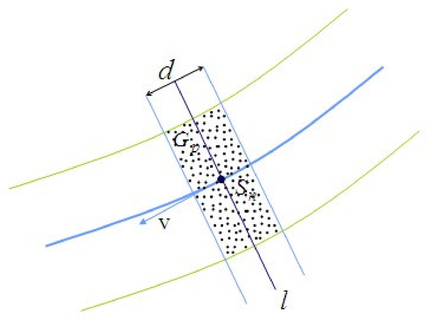
The cross-section $l$ is estimated from point $S_n$, perpendicular to the normal vector $S_{n}V$. Here, $S_{n}V$ is the vector of the normal plane at point $S_n$ in the centerline. To generate the cross-section, point group $G_p$ is extracted from two planes that are parallel to plane $l$ at distance $d$. Then, by projecting point group $G_p$ onto plane $l$, the final cross-section, consisting of a series of points, can be obtained (Figure 8).

4. Experiment

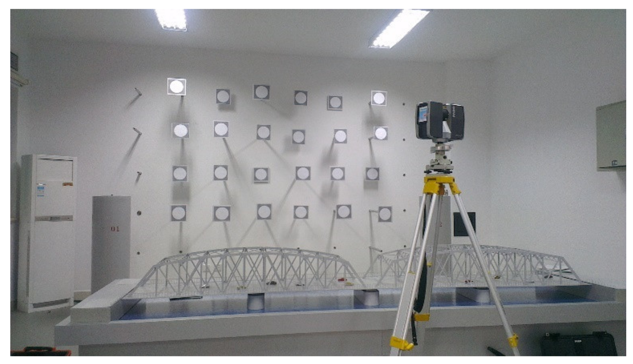
The proposed method is applied to a real shield tunnel. The scanner used in the experiment is a FARO Focus3D150s, and the accuracy (single measurement) is 2 mm@25 m. For comparison, the tunnel is surveyed again with a total station (TS) of SOKA SET1130R3 (±1′). The test tunnel site is illustrated in Figure 9. This section has a total length of 170 m and 6 scanning stations.

The OMTLS method is used in the tunnel to rapidly register the point clouds from the multi-view. Figure 10a illustrates the implementation of OMTLS. First, an accurate and reliable control network is laid in the tunnel to control the error propagation, and the coordinate of each control point in the control network is obtained before scanning. As for the practice of the control network layout, which is according to the requirements of second-class precision measurement, the edges and corners of the connecting traverse are observed to conduct a coordinate computation of unknown control points (Figure 10b). Second, the target ball, which serves as the tie point, is set above the control point. Thus, the coordinate of the target ball is equal to the control point lying beneath it. In practice, the target ball should be arranged within the range of laser scanning, and the optical distance from the laser scanner should be less than 10 m.

Before scanning, with the help of the total station, $T_1$ and $T_2$ (Figure 2) are directly measured to compute the coordinates of $O^{\prime }$. With the OMTLS method, the point clouds obtained in each scan can be directly transformed into the reference system, to constitute the tunnel point clouds. Moreover, the cell box compression method can be implemented immediately to reduce the point clouds to an appropriate level for further use.

The number of points is reduced to (100,870) after data compression. The improved MLS technique is further adopted to thin the point clouds with h = 1 and two iterations. To thin the point clouds, the voxel cell method [30] is used to reduce the point set to 164 points. Then, the points are approximated with a quadratic B-spline curve with 58 control points (Figure 6c) by using the chord-length parameterization scheme.

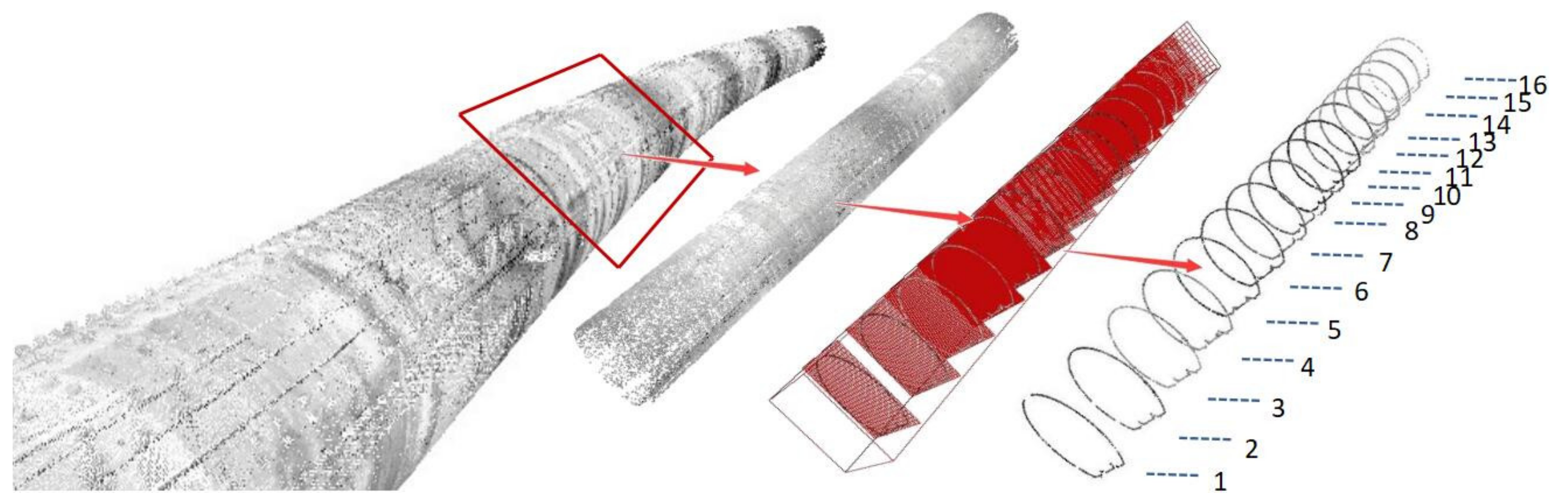
Cross-sections are generated using the proposed method, as illustrated in Figure 7. Figure 11 presents the generation of the cross-sections. To meet the accuracy requirement, the distance $d$ selected here is 20 cm, which can achieve a good result. In general, the selection of distance $d$ should be associated with the curvature of the centerline. If $d$ is too large, an inaccurate cross-section will be generated. If $d$ is too small, the computation time will increase, thereby making the process inefficient.

The least-squares method is utilized to fit the points in the cross-section to a circle and compute the convergence of the cross-section. Tunnel deformation can be directly reflected by comparing the change in the radius with the reference value. For the reference value, by using a total station, each cross-section was surveyed by observing 11 points at ${20}^{\circ }$ intervals from ${-10}^{\circ }$ to ${190}^{\circ }$ at each station. The initial cross-section must be marked with target planes, and it can serve as a correspondence to the initial attitude of the cross-section, generated from the point clouds. Part of the cross-sections is selected for comparison with the data from the total station and the design values.

Table 1. Comparison of values obtained by different methods with the same design values.

Cross-Section ID	Number of Points		Radius of the Circle (m)		Δ(Dev) (m)
	TLS	TS	TLS	TS	TLS	TS
1	3224	11	2.7432	2.7450	−0.0068	−0.0050
2	3524	11	2.7451	2.7460	−0.0049	−0.0040
3	3328	11	2.7417	2.7430	−0.0083	−0.0070
4	3494	11	2.7462	2.7450	−0.0038	−0.0050
5	3501	11	2.7467	2.7490	−0.0033	−0.0010
6	3568	11	2.7451	2.7470	−0.0049	−0.0030
7	3329	11	2.7417	2.7430	−0.0083	−0.0070
8	3493	11	2.7471	2.7450	−0.0029	−0.0050
9	3506	11	2.7514	2.7490	0.0014	−0.0010
10	3602	11	2.7528	2.7520	0.0028	0.0020
11	3492	11	2.7540	2.7520	0.0040	0.0020
12	3549	11	2.7451	2.7470	−0.0049	−0.0030
13	3521	11	2.7472	2.7480	−0.0028	−0.0020
14	3411	11	2.7524	2.7510	0.0024	0.0010
15	3379	11	2.7483	2.7490	−0.0017	−0.0010
16	3318	11	2.7456	2.7470	−0.0044	−0.0030
RMSE					0.0047	0.0038

shows the comparison of different methods.

For comparison, 16 cross-sections (as shown in Figure 11) are selected as analysis targets. After obtaining the points of the cross-sections, the least-squares method is implemented to fit the points and produce an optimal circle. Table 1 shows that the final cross-sections from the proposed method include more points than those taken from the total stations. This result indicates that the proposed method provides a more detailed description of the tunnel profile. Meanwhile, the proposed method can obtain a more reliable result during the least-squares iteration. To reveal the convergence changes, the radius is compared with the design value. Here, the design radius of the shield tunnel is 2.75 m. After fitting an optimal circle, the cross-sections estimated by the proposed method and the total station are compared in Table 1. The RMSE of the TLS method is estimated as 0.0047 m, and the corresponding value of the total station is estimated as 0.0038 m. The accuracy of the TLS method is slightly lower than that of the total station, but TLS is more efficient than the total station with respect to data acquisition and processing. At the same time, the data from the total station are mainly dependent on artificial selection and are therefore easily influenced by poor inner tunnel conditions.

Figure 12 shows the analysis of deviation. The red line signifies the discrepancy from the total station, and the blue line indicates the Dev from TLS. The two lines exhibit the same trend in this section. The main change for TLS occurs in IDs 3 and 7, which is consistent with the trend of the total station. The segments from IDs 7 to 11 have the largest relative changes, indicating that these parts have severe deformation. This deviation phenomenon can be clearly reflected by the two methods.

The data collection and processing times are summarized in

Table 2. Consumption times.

Categories	TLS		Total Station
	Activities	Times (min)	Activities	Times (min)
Data surveying	Control network layout	30	Instrument installation	102 (= 3 * 34 stations)
	PB parameter acquisition	24 (= 4 * 6 stations)	Cross-section surveying	170 (= 5 * 34 stations)
	Inside scanning	24 (= 4 * 6 stations)
Data processing	Data transform	<1	Data fitting	<2
	Medial axis generation	<3	Results	2
	Final cross-section generation	<2
	Results	2
Total		86		276

. Most of the time is spent on data collection, whereas data processing consumes less time. The data acquisition of TLS involves three main items, and the total time taken is about 78 min. In contrast with TLS, the total station involves two activities, which appear to be more time-consuming (238 min) than those of TLS. The overall time cost of the proposed method is estimated to be less than one-third of that of the total station survey. The gap is expected to widen when the number of cross-sections is increased. The item in the present method that has the largest time cost is the control network layout, which is a conventional task in tunnel monitoring. The scanning time is expected to decrease greatly with the development of new hardware.

5. Conclusions

Although TLS has been widely utilized in engineering surveying projects, wider application in the fields of deformation monitoring, especially in the tunnel-monitoring arena, still faces many obstacles, such as extensive metadata processing and low-accuracy data analysis. This paper presents a systematic method for tunnel deformation analysis based on point clouds. The results of the proposed method were compared with the conventional method. In this study, OMTLS was proposed for the fast registration of point clouds, and a PB model was designed for the acquisition of transformation parameters. Meanwhile, an improved MLS was introduced as a way to thin point clouds and obtain the centerline of a tunnel. Cross-sections were rapidly produced, based on the centerline. The proposed method was then applied to a real shield tunnel in practice. The results proved that TLS is appropriate for use in tunnel monitoring. Moreover, the cross-sections generated from the point clouds were described in detail. The proposed method was determined to be highly efficient in terms of data acquisition and processing times. Overall, the results confirmed that the proposed method is efficient and can meet the accuracy requirements of tunnel monitoring.

In the future, the possibility of applying the proposed method to other tunnel types, such as excavation and irregular tunnels, will be explored. The images obtained using TLS were not discussed in this study, but they could play an important role in the inspection of cracks and water seepage during tunnel monitoring. This subject could also be a key direction for future research.

References

- Mukupa, W.; Roberts, G.W.; Hancock, C.M.; Al-Manasir, K. A review of the use of terrestrial laser scanning application for change detection and deformation monitoring of structures. Surv. Rev. 2016, 49, 99–116. [Google Scholar] [CrossRef]
- Wang, T.-T.; Jaw, J.-J.; Hsu, C.-H.; Jeng, F.-S. Profile-image method for measuring tunnel profile—Improvements and procedures. Tunn. Undergr. Space Technol. Inc. Trenchless Technol. Res. 2010, 25, 78–90. [Google Scholar] [CrossRef]
- Gikas, V. Three-Dimensional Laser Scanning for Geometry Documentation and Construction Management of Highway Tunnels during Excavation. Sensors 2012, 12, 11249–11270. [Google Scholar] [CrossRef] [PubMed] [Green Version]
- Kang, Z.; Zhang, L.; Tuo, L.; Wang, B.; Chen, J. Continuous Extraction of Subway Tunnel Cross Sections Based on Terrestrial Point Clouds. Remote. Sens. 2014, 6, 857–879. [Google Scholar] [CrossRef] [Green Version]
- Lague, D.; Brodu, N.; Leroux, J. Accurate 3D comparison of complex topography with terrestrial laser scanner: Application to the Rangitikei canyon (N-Z). Isprs J. Photogramm. Remote. Sens. 2013, 82, 10–26. [Google Scholar] [CrossRef] [Green Version]
- Fekete, S.; Diederichs, M.; Lato, M. Geotechnical and operational applications for 3-dimensional laser scanning in drill and blast tunnels. Tunn. Undergr. Space Technol. Inc. Trenchless Technol. Res. 2010, 25, 614–628. [Google Scholar] [CrossRef]
- Xu, X.; Yang, H.; Neumann, I. Time-efficient filtering method for three-dimensional point clouds data of tunnel structures. Adv. Mech. Eng. 2018, 10, 168781401877315. [Google Scholar] [CrossRef] [Green Version]
- Han, J.Y.; Guo, J.; Jiang, Y.S. Monitoring tunnel profile by means of multi-epoch dispersed 3-D LiDAR point clouds. Tunn. Undergr. Space Technol. Inc. Trenchless Technol. Res. 2013, 33, 186–192. [Google Scholar] [CrossRef]
- Lam, S. Application of terrestrial laser scanning methodology in geometric tolerances analysis of tunnel structures. Tunn. Undergr. Space Technol. Inc. Trenchless Technol. Res. 2006, 21, 410. [Google Scholar] [CrossRef]
- Huang, S.; Chen, M.; Lu, S.; Chen, S.; Zha, Y. A novel algorithm: Fitting a spatial arc to noisy point clouds with high accuracy and reproducibility. Meas. Sci. Technol. 2021, 32, 085004. [Google Scholar] [CrossRef]
- Besl, P.J. A method for registration of 3d shapes. IEEE Trans. PAMI 1992, 14, 239–256. [Google Scholar] [CrossRef]
- Yang, C.; Medioni, G. Object modeling by registration of multiple range images. Image Vis. Comput. 2002, 10, 145–155. [Google Scholar]
- Mitra, N.J.; Gelfand, N.; Pottmann, H.; Guibas, L. Registration of Point Cloud Data from a Geometric Optimization Perspective. In Proceedings of the 2004 Eurographics Symposium on Geometry Processing, Nice, France, 8–10 July 2004. [Google Scholar]
- Gelfand, N.; Ikemoto, L.; Rusinkiewicz, S.; Levoy, M. Geometrically Stable Sampling for the ICP Algorithm. In Proceedings of the Fourth International Conference on 3-D Digital Imaging and Modeling, Banff, AB, Canada, 6–10 October 2003. [Google Scholar]
- Fitzgibbon, A.W. Robust registration of 2D and 3D point sets. Image Vis. Comput. 2001, 21, 1145–1153. [Google Scholar] [CrossRef]
- Jost, T.; Hugli, H. A multi-resolution ICP with heuristic closest point search for fast and robust 3D registration of range images. In Proceedings of the Fourth International Conference on 3-D Digital Imaging and Modeling, Banff, AB, Canada, 6–10 October 2003. [Google Scholar]
- Higuchi, K.; Hebert, M.; Ikeuchi, K. Building 3-D Models from Unregistered Range Images. Graph. Models Image Process. 1995, 57, 315–333. [Google Scholar] [CrossRef] [Green Version]
- Robotique, P.; Epidaure, P.; Feldmar, J. Locally Affine Registration of Free-Form Surfaces. In Proceedings of the IEEE Conference on Computer Vision and Pattern Recognition, Seattle, WA, USA, 21–23 June 1994. [Google Scholar] [CrossRef]
- Wyngaerd, J.V.; Van Gool, L.; Koch, R.; Proesmans, M. Invariant-based registration of surface patches. In Proceedings of the Seventh IEEE International Conference on Computer Vision, Kerkyra, Greece, 20–27 September 1999. [Google Scholar]
- Mclain, D.H. Drawing Contours from Arbitrary Data Points. Comput. J. 1974, 17, 318–324. [Google Scholar] [CrossRef]
- Mclain, H. Two Dimensional Interpolation from Random Data. Comput. J. 1976, 19, 178–181. [Google Scholar] [CrossRef] [Green Version]
- Amenta, N.; Kil, Y.J. The Domain of a Point Set Surfaces. Eurographics Symposium on Point-based Graphics. 2004. Available online: https://escholarship.org/uc/item/94s9d3x6 (accessed on 29 July 2021).
- Shen, C.; O’Brien, J.F.; Shewchuk, J.R. Interpolating and approximating implicit surfaces from polygon soup. ACM Transactions on Graphics 2004, 896–904. [Google Scholar] [CrossRef] [Green Version]
- Guennebaud, G.; Germann, M.; Gross, M. Dynamic Sampling and Rendering of Algebraic Point Set Surfaces; John Wiley & Sons, Ltd.: Hoboken, NJ, USA, 2010; pp. 653–662. [Google Scholar]
- Guennebaud, G.; Gross, M. Algebraic Point Set Surfaces. ACM Trans. Graph. 2007, 26, 23-es. [Google Scholar] [CrossRef]
- In-Kwon, L. Curve reconstruction from unorganized points. Computer Aided Geometric Design 2000, 17, 161–177. [Google Scholar]
- Alexa, M.; Behr, J.; Cohenor-Or, D.; Fleishman, S.; Levin, D.; Silva, C.T. Point set surfaces. In Proceedings of the IEEE Visualization, San Diego, CA, USA, 21–26 October 2001. [Google Scholar]
- Levin, D. Mesh-Independent Surface Interpolation; Springer: Berlin/Heidelberg, Germany, 2004. [Google Scholar]
- Hoschek, J.; Lasser, D. Fundamentals of Computer Aided Geometric Design. Math. Comput. 1996. [Google Scholar] [CrossRef]
- Yang, Z.; Ruess, M.; Kollmannsberger, S.; Düster, A.; Rank, E. An efficient integration technique for the voxel-based finite cell method. Int. J. Numer. Methods Eng. 2012, 91, 457–471. [Google Scholar] [CrossRef] [Green Version]
Figure 1.
Flow diagram of the proposed method.