Article

Towards High-Resolution Land-Cover Classification of Greenland: A Case Study Covering Kobbefjord, Disko and Zackenberg

by
Daniel Alexander Rudd
1,2,
Mojtaba Karami
3 and
Rasmus Fensholt
1,*
1
Department of Geosciences and Natural Resource Management, University of Copenhagen, 1350 Copenhagen, Denmark
2
Department of Bioscience, Aarhus University, 4000 Roskilde, Denmark
3
BASF Digital Farming GmbH, Im Zollhafen 24, 50678 Cologne, Germany
*
Author to whom correspondence should be addressed.
Remote Sens. 2021, 13(18), 3559; https://0-doi-org.brum.beds.ac.uk/10.3390/rs13183559
Submission received: 12 August 2021 / Revised: 31 August 2021 / Accepted: 2 September 2021 / Published: 7 September 2021
(This article belongs to the Special Issue Advances in Terrestrial Remote Sensing of Arctic Environments)

Abstract

:
Mapping of the Arctic region is increasingly important in light of global warming as land cover maps can provide the foundation for upscaling of ecosystem properties and processes. To this end, satellite images provide an invaluable source of Earth observations to monitor land cover in areas that are otherwise difficult to access. With the continuous development of new satellites, it is important to optimize the existing maps for further monitoring of Arctic ecosystems. This study presents a scalable classification framework, producing novel 10 m resolution land cover maps for Kobbefjord, Disko, and Zackenberg in Greenland. Based on Sentinel-2, a digital elevation model, and Google Earth Engine (GEE), this framework classifies the areas into nine classes. A vegetation land cover classification for 2019 is achieved through a multi-temporal analysis based on 41 layers comprising phenology, spectral indices, and topographical features. Reference data (1164 field observations) were used to train a random forest classifier, achieving a cross-validation accuracy of 91.8%. The red-edge bands of Sentinel-2 data proved to be particularly well suited for mapping the fen vegetation class. The study presents land cover mapping in the three study areas with an unprecedented spatial resolution and can be extended via GEE for further ecological monitoring in Greenland.

Graphical Abstract

1. Introduction

Arctic studies are increasingly relevant in the scope of climate change as the region’s seasonal variables provide important information on the global climate system [1]. Despite their importance, the vast landscapes are sparsely populated and difficult to reach; hence, large-scale comparative studies of landscape elements are limited. Mapping of the biophysical cover of Arctic surfaces is fundamental for monitoring purposes and form an important basis for studies of various ecosystem processes and states such as greenhouse gas exchange [2,3,4], surface energy balance [5,6], and permafrost [7,8]. These interactions are often measured on a local scale, but to interpret their influence in a regional context, it is essential to identify the physical extent of the land cover. This is where improved technology of satellite images provides an easily accessible tool to map the Arctic land cover from above.
Working with land-cover classification based on large amounts of data with high dimensionality increases the need for processing power [9,10,11]. To assist the remote sensing community with the necessary processing power, the use of cloud computing platforms such as Google Earth Engine (GEE) is an extremely valuable tool. GEE is a cloud-based platform consisting of a large data catalog from different satellite sources and spatial analysis tools. It is operated through a web-based application programming interface (API) [12]. With no need for manual download of satellite images or a powerful desktop at the user end, this platform provides the user with the necessary tools for processing large amounts of data relatively quickly. The rapid response to changes in the analysis gives the user the ability to evaluate the output more easily. This geospatial analysis platform is free to use, and it is considered to be state-of-the-art for remote sensing analysis [9,10,12,13,14].
Maps of vegetation characteristics exist for Greenland as part of circumpolar arctic vegetation classification efforts [15,16,17] based on a blend of information, including also satellite imagery and the Circumpolar Arctic Vegetation Map (CAVM) [16], and is provided in a 1 km spatial resolution. Karami et al. [18] produced a spatially more detailed vegetation land-cover map for all of the ice-free parts of Greenland, utilizing data from the Landsat 8 OLI satellite, representing current state-of-the-art in land-cover mapping of Greenland. Their rationale behind surface classes for their land-cover classification was similar to previous upscaling applications in Greenland, and the map should, therefore, be suitable for such use [18]. Their work relied on time-series analysis of 2015 Landsat data, producing per-pixel vegetation phenology metrics, Normalized Difference Moisture Index (NDMI), and topography features combined with a Random Forest (RF) classifier. With more than 4000 Landsat 8 images, this work was a very time-consuming process [18]. Their complete regional land-cover map of the ecosystems in Greenland in a 30 m resolution is to the author’s knowledge the only of its sort in such a high resolution.
With the rapid technological development and an increase in available data sources, the remote sensing community is provided with an increasing number of opportunities to further improve their research. On this basis, this article aims to optimize the work of Karami et al. [18] by utilizing imagery from newer satellites in combination with cloud computing.
While Sentinel-2 and Landsat 8 are relatively similar regarding spectral resolution, there is one region of the electromagnetic spectrum that is further collected by the Sentinel-2 satellites; the red-edge. This spectral region is located between the red and the NIR wavelengths and vegetation is spectrally characterized by a sharp increase in this spectral region [19]. The use of information gained from the red-edge has shown to be important for vegetation discrimination due to its sensitivity to e.g., the vegetation’s structural characteristics [20].
The study of vegetation phenology based on remote-sensed optical imagery commonly relies on vegetation indices (VI). One of the most used VI is the Normalized Difference Vegetation Index (NDVI), which relies on the relative difference between the red and near-infrared (NIR) wavelengths. This index has been shown to correlate with several vegetation characteristics such as biomass, leaf area index, and carbon fluxes [21,22]. Time-series of NDVI values are commonly used to describe the vegetation phenology, thereby extracting metrics related to the growing season [23]. While it might be possible to partly distinguish types of vegetation solely on phenology timing and peak NDVI, studies have shown that including topography information and other spectral indices, such as the NDMI, increases classification accuracy [18,24]. With the timing of green-up and senescence derived from the phenology analysis, it is possible to examine the vegetation’s spectral signature within its growing season.
Classification based solely on optical images has caused problems when different land covers have had similar spectral signatures. One problem of such observation is the spectral similarity of water and shadows [25,26]. The solar reflectance of these areas is close to zero, which makes them difficult to distinguish from each other. To overcome this problem some studies have proposed water indices that increase the small spectral differences [27,28], while others have strived to incorporate information about the topography in combination with the illumination conditions at the time of observation [25,26]. While there is no comprehensive solution to this challenge, the methodological approach should depend on the conditions in the area of interest.
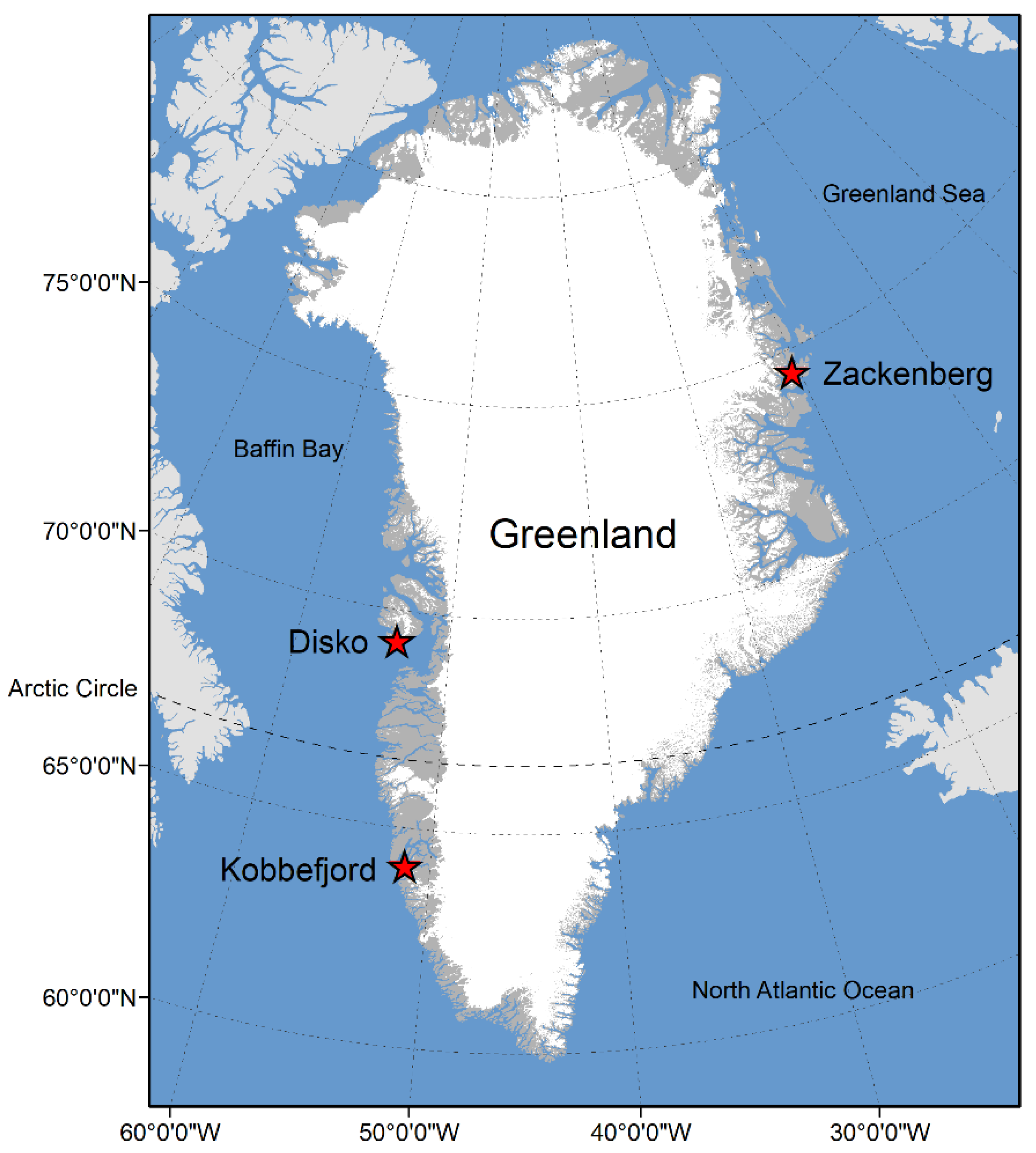
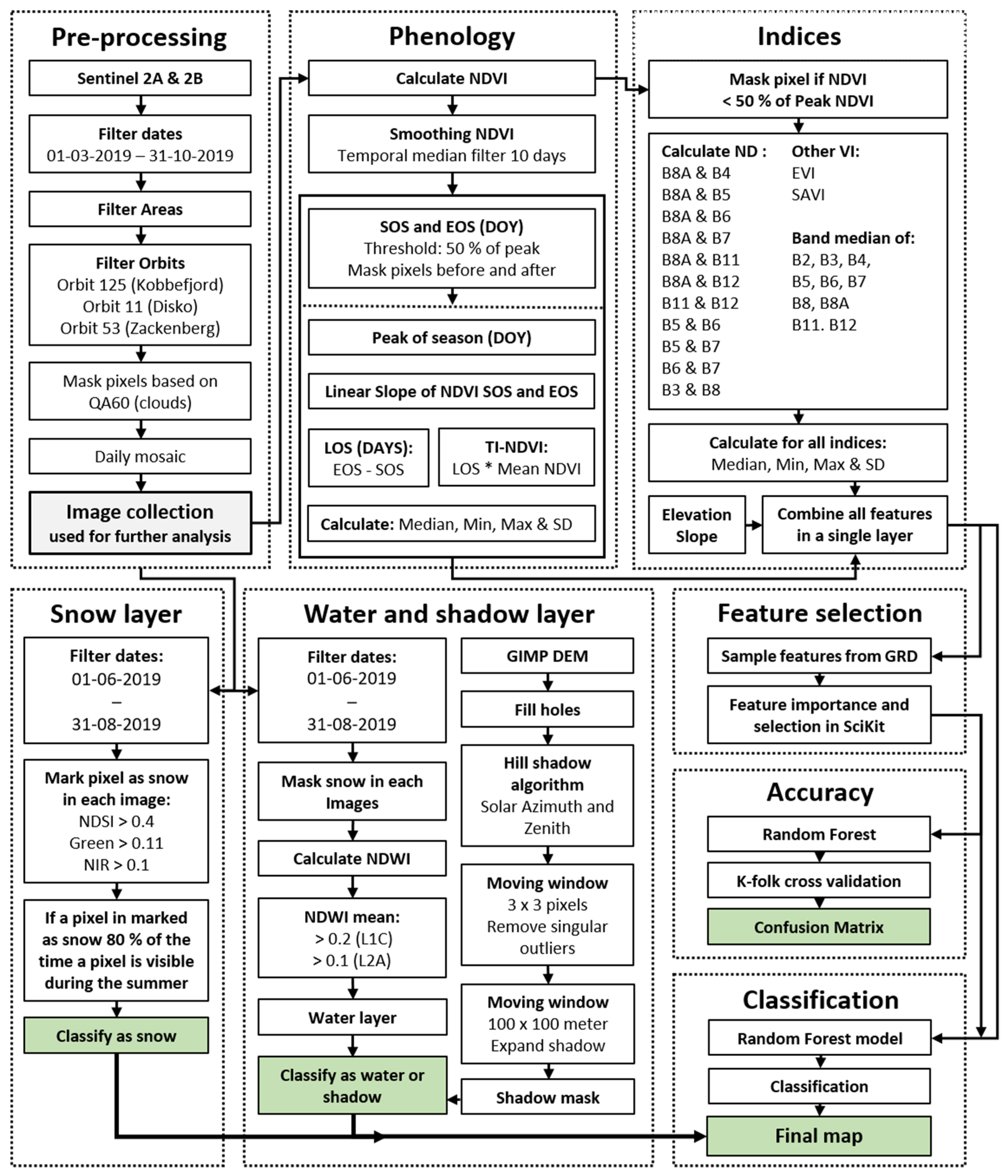
This study seeks to produce high-resolution land-cover maps for selected parts of Greenland using multi-temporal images from the Sentinel-2 satellites. The study provides the basis for further improving the classification scheme presented by Karami et al. [18]. The new classification is based on phenological metrics from NDVI time-series, wetness estimation based on NDMI; indices including information obtained from the red-edge bands, topographical features, and in situ observations are included to train the Random Forest classifier [29]. The extracted features are analyzed for their importance related to the classifier and their ability to separate vegetation land-cover classes. A water detection workflow, based on water indices in combination with a hill shadow algorithm, is built to automatically map water-covered areas. This whole framework for land cover classification is coded in GEE.
This study, thereby, aims to provide a methodology to produce high-resolution land-cover maps that could be utilized for further Arctic research.

2. Materials and Methods

2.1. Study Sites

Greenland stretches 2500 km from 60°N to 82°N, and a large ice sheet covers approximately 80% of the terrestrial surface. The remaining 20% or 425,000 km2 ice-free land along the coast of Greenland is mostly covered by tundra vegetation, inland water bodies, and barren surfaces [18]. The study sites are located in three ice-free areas of Greenland; Kobbefjord, Disko, and Zackenberg, as illustrated in Figure 1.
While all three study sites are located within the Arctic climate zone, they differ in their locations which influence the climatic conditions in each site (Table 1). Kobbefjord, located in the Low Arctic climate zone, is characterized by a mean annual temperature of −0.9 °C, annual precipitation of 782 mm, and no permafrost. Secondly, also located on the West coast of Greenland is Disko; this study site has a lower mean annual temperature, lower annual precipitation, and experiences discontinuous permafrost. Its climate zone is therefore defined as somewhat in-between the Low and High Arctic. The third study site, Zackenberg, is located on the East coast within the High Arctic climate zone. Here, the mean annual temperature and total annual precipitation are the lowest of the three sites, and the site exhibits continuous permafrost [30].
Temperature and precipitation are key elements for plant growth [31], and the variation between the three sites consequently results in different land covers [18,32]. Following Table 1 it is therefore assumed that the High Arctic would have less favorable conditions for vegetation growth than the Low Arctic.
The rationale for choosing these three sites lies in their participation in the Greenland Ecosystem Monitoring (GEM) programme, and research has thus been conducted in the three study sites for many years. This has consequently enabled access to in-situ observations and high-resolution drone images of these areas which in turn has increased the validity of the ground reference data (GRD). Based on Karami et al. [18] these are the three areas with the most GRD, while still being located in different climate zones. This makes the areas appropriate as study areas to examine the potential of creating a scalable classification framework with the ability to classify the three areas simultaneously under the same premises.

2.2. Data

2.2.1. Sentinel-2

The optical satellite images are collected by the two identical Sentinel-2 satellites, which are part of the Copernicus program. The first satellite, Sentinel-2A, was set in orbit around the Earth in June 2015, while the second one, Sentinel-2B, was launched in March 2017. These satellites are put in sun-synchronous orbits and are operating simultaneously phased at 180 degrees to one another. Each satellite has a revisiting time of 10 days at the equator and including both results in a temporal resolution of 5 days [33]. Both satellites are mounted with a Multi-Spectral Instrument (MSI), which is an optical sensor working passively by collecting the reflection of sunlight from the Earth at 13 different spectral bands. The spatial and spectral resolution of the 13 bands can be seen in Table S1.
The images used for the image classification were the L1C product, which provides top-of-atmosphere reflectance. Before being released as an L1C product, the raw images go through several processing steps, e.g., conversion to top-of-atmosphere reflectance and a geometric correction [33]. Although the Bottom of Atmosphere (L2A) product is available in GEE, it has, unfortunately, been shown to have incorrect reflectance values for a certain number of pixels in the Arctic. These errors alter the NDVI, making them problematic to include in an automated phenology analysis (Figure S1).

2.2.2. Digital Elevation Model

The DEM used for both the vegetation classification and the water/shadow algorithm was obtained from the Greenland Mapping Project (GIMP). The GIMP DEM is constructed on a combination of three different sources; ASTER, SPOT-5, and AVHRR photoclinometry. It covers all of Greenland, including both the ice sheet and ice-free areas, with a spatial resolution of 30 m [34].

2.2.3. Ground Reference Data

The GRD used as input for the vegetation classification is based on the GRD used in Karami et al. [18], intersecting with the three areas of interest (Figure 1). Some points were obtained during the field campaigns of Karami et al. [18] in 2015, while others were interpretations of the two vegetation transects located in Kobbefjord and Zackenberg. Moreover, points were further created by exploring high-resolution satellite and drone images [18]. An additional 129 GRD points, based on inspection of high-resolution drone imagery available through the Greenland Ecosystem Monitoring database, have been added to the dataset. The GRD consists of six different classes (Table 2; examples of the six surface classes are illustrated in Figure S2).
A spatial analysis was conducted to make sure no points were within 15 m of each other as they could potentially fall within the same pixel. An overview of GRD points per class and case area is given in Table 3 (the spatial distribution can be seen in Figure S3).

2.3. Classification Workflow

2.3.1. Preprocessing and Masking for Snow, Water and Shadows

The chosen period includes 560 Sentinel-2 images acquired between early March 2019 and end of October 2019 (Figure 2; pre-processing). To include as much useful information as possible, each image was passed through a cloud masking algorithm instead of being excluded based on the total cloud cover. The cloud masking algorithm was built upon the quality assessment band (QA60), which detects pixels of low quality due to the presence of either dense or cirrus clouds [33].
Snow cover was identified similarly to the automated snow detecting algorithm used in the MODIS global snow cover product [35]. This algorithm consists of three different thresholds and a pixel has to meet all three criteria to be classified as snow-covered (Figure 2; snow layer) [35]. If a pixel is classified as snow-covered in >80 % of the instances during the summer period June–August, it is classified as snow in the final map. The Normalized Difference Water Index (NDWI) was used to detect possible water pixels [36]. For a pixel to be considered water-covered, it must pass two NDWI based thresholds (Figure 2; water layer). For this part of the analysis, the L2A product was found to be a benefit to include due to the initial reductions of misclassified shadow areas by the topographical correction. These thresholds are based on the mean NDWI value throughout the chosen period. These thresholds were found by trial-and-error, where different thresholds were examined through visual inspection in areas where high-resolution satellite images were available. Although the inclusion of the L2A, in this part, did reduce the misclassification of shadow areas as water, it did not exclude all of them. Therefore, a GEE built-in algorithm called Hillshadow was used to create a layer of possible shadow areas based on a DEM, solar zenith angle, solar azimuth angle, and a neighborhood size (Figure 2; shadow layer). The algorithm projects light rays over a DEM based on the input illumination conditions, thereby analyzing every pixel for light occlusion in a straight line towards the sun. Only the pixels which are classified as both potential water and potential shadow are assigned to the shadow class, while the remaining potential water areas are classified as water in the final classification.

2.3.2. Phenology Metric Extraction

Studying phenology based on multi-temporal satellite imagery typically relies on a temporal analysis of a vegetation index such as NDVI [23]. In order to remove residual noise from inaccuracies in the cloud QA band, a smoothing algorithm was applied based on a non-parametric median filter function. This algorithm iterates through the image collection on a pixel-by-pixel basis and calculates the median of 10 days (Figure 2; phenology). A relative threshold level of 50% of the peak NDVI was used to indicate both the start of season (SOS) and end of season (EOS). Based on these two dates, the algorithm masks out all pixels taken before SOS and after EOS, for that specific pixel. The length of the growing season (LOS) is defined as the difference between SOS and EOS. A simplified time-integrated NDVI (TI-NDVI) is calculated based on the mean NDVI of all the smoothed NDVI values within the defined growing season, multiplied with the LOS. The peak of the season was defined as the mean day of year (DOY), where the smoothed NDVI was above 90% of the peak. The growing rate at the beginning of the season was linearly defined as the daily NDVI change rate from the first point of SOS until the first observation above 90% of the peak. Likewise, the slope at the end of the season was defined as the daily change rate from the last observation in the peak season until the last observation of the growing season. Within the growing season, the median, minimum (min), maximum (max), and standard deviation (SD) of NDVI were calculated, creating a set of 13 phenology metrics.

2.3.3. Spectral Indices and Topography Derivate

The number of observations to include in the calculation of spectral indices (Figure 2; Indices) also relied on the phenology (2.3.2). In addition to masking out all observations before and after the growing season, the algorithm masks out all observations with a NDVI value below the relative threshold. This assists in removing sudden drops below the threshold during the growing season that are most likely caused by clouds or cloud shadows not identified by the cloud mask. The number of observations within the defined growing season for the three case areas (Figure S4) showed that surfaces covered with vegetation predominantly result in 11–25 observations within the growing season. This indicates that a sufficient number of high-quality observations was obtained after the removal of erroneous values [from each pixel time series] using this approach.
The computed indices include the classical ones such as EVI, SAVI, NBR, NBR2, and NDWI. Moreover, we included multiple indices based on the three red-edge bands. First, a set of indices where the red band, which is originally used in NDVI, was replaced with the red-edge bands. This creates three new VI’s which are based on sequences of the narrow NIR band and each of the red-edge bands (Table 4). Additionally, normalized differences of the red edge bands were calculated in three combinations. All of the indices were calculated for each pixel in all scenes throughout the defined growing season, following statistical feature extraction such as median, minimum, maximum, and standard deviation. Each index, therefore, results in four features, for a total of 52 features. Furthermore, extraction of the median reflectance value during the growing season was performed for bands 2–8A, 11, and 12.
The elevation (from the GIMP DEM) was used as a feature itself, and also used to calculate the slope of the terrain at three different scales; one where the original elevation was used, and two others where the original elevation had been passed through a moving window of 100 m and 200 m, respectively, before calculating the slope. This moving window assigns a new elevation to each pixel, based on the mean elevation of the surrounding pixels. The subsequently calculated slopes would, therefore, be a more smoothed and general description of the topography.

2.3.4. Vegetation Classification and Validation

All of the above-described features were calculated and stacked together in a single data file comprising of 79 different layers representing each feature (Table S2) covering the three study areas to be able to build a single model covering all three areas.
The vegetation classification was performed with an RF classifier [29], being amongst the built-in classifiers in GEE. RF is a non-parametric supervised ensemble classifier which is based on the same fundamental principles as Classification And Regression Trees (CART) and the bootstrapping aggregation approach (Bagging) [43]. The RF classification approach builds a large collection of binary decision trees, where each tree is trained using a randomly selected subset from the full training data set [44]. These subsets usually consist of 2/3 of the full training set, while the remaining 1/3 is utilized as an internal validation, known as the out-of-bag error (OOB error). The number of trees (Ntree) was set to 500, as it has been demonstrated to be a sufficient number of trees to flatten out the OOB error curve, and increasing this number beyond 500 showed minor changes in the accuracy [43]. It is also the suggested value to use for remotely sensed data [44]. The number of the randomly selected features per node split (Mtry) was set to the default of the square root of total features. Each tree was grown to full depth.
All the GRD were uploaded to GEE, and each point was used to sample the features (Figure 2; Feature selection). These sampled values were then exported from GEE and imported into the Scikit-learn phyton package for an examination of the individual feature importance. The 1164 GRD points utilized to sample the 79 features from phenology, indices, band medians, and topography produced 91,956 sampled values used for the feature analysis. The procedure in this feature selection package relies on the recursive feature elimination principle combined with cross-validation (RFECV) to search for the optimal combination of features yielding the highest overall accuracy (OA). To examine the effect of the red-edge bands in the classification, the RFECV was performed on two sets of features: (i) A RFECV analysis where all the 79 features were available; and (ii) a RFECV analysis where all features that include any red-edge bands were excluded, which generated a subset of 53 features.
A k-fold cross-validation was employed to assess the accuracy of the RF classifier and validate the results of the land-cover classification (Figure 2; Accuracy). K-fold CV is a resampling algorithm that randomly resamples all the reference data into equally sized stratified subsets (folds) [43] and for each round of cross-validation, one fold is kept out and subsequently used as validation, while the remaining folds are used for training. This cross-validation was repeated ten times, withholding a different fold for each repetition, thus allowing all reference data to be used for both training and validation.
The classification accuracy was estimated using contingency (confusion) matrices. We calculated the area-weighted overall, producer, and user’s accuracies for each class. We also calculated error-adjusted area estimates and the proportion of each class based on the results of accuracy assessments following state-of-the-art accuracy assessment recommendations [45,46]. A non-parametric McNemar’s test with continuity correction was used to determine if statistically significant differences in the performance of classifications (p = 0.05) based on different models (i.e., with or without red-edge bands) were obtained [47,48].

3. Results

3.1. Feature Importance

Analyzing the relationship between the number of features included in the RF classifier and the changes in CV scores demonstrates that the majority of the information can be found in the most important features (Figure 3). It is observed that relatively high accuracies are reached when including only the three most important features. When including more than 20 features, the accuracy curve flattens, and only small changes in the accuracy are achieved from this point. Nevertheless, the RFECV analysis found that the highest OA was reached when including 41 features, indicating that the 38 features with the lowest importance could be excluded without any loss in OA.
The feature importance analysis (Figure 4) revealed that 9 of the 13 features from the phenology analysis were part of the 41 features. The TI-NDVI was the feature of the highest importance, while NDVI median and NDVI max were part of the ten most important features. The second most important feature was the maximum value from the VI RE2, which is based on the Narrow NIR (865 nm) and the second red-edge band (740 nm). The analysis reveals that five out of the ten most important features include information gained from the second (740 nm) and third (783 nm) red-edge bands. Such an observation indicates the effectiveness of including features based on the red-edge bands in relation to vegetation classification in an Arctic setting. Fourteen features that contain the red-edge bands were part of the top 41.
The median values of the three visual bands and the two SWIR bands, were part of the top 41, with the blue band being part of the top 10 most important features. For the topographical features, the elevation, slope100, and slope200 were found to be of some importance for the classification, with elevation being the most important of the three. As GEE allocates ample processing power, it was chosen to build the RF classifier on the optimal combination of 41 features.

3.2. Image Classification and Validation

The final classified land-cover maps were constructed by stacking the three classified layers; snow, water/shadow, and vegetation (Figure 5) (maps can be seen in a full-page format in Figures S5–S7). Of general observations across all three extents is the decrease in vegetation cover with higher altitudes. Zooming in on each of the three key areas, it is demonstrated how the high spatial resolution of the classified maps has been able to classify the land covers without a considerable salt-and-pepper effect. It further shows how the three sites differ in types of land cover, where Kobbefjord and Disko have substantially more areas of wet heath and copse/tall shrubs, compared to Zackenberg where these two land cover classes are absent.
The analysis revealed that the percentage of the ground being barren increased from Kobbefjord to Disko to Zackenberg, which indicates a decrease in vegetation cover towards the higher latitudes (Table 5). The analysis further showed a decrease in areas covered by the two classes of wet heath and dry heath/grassland towards northern latitudes. Copse and tall shrubs were consistently the land cover class with the least prevalence, followed by the fen class. The distribution of land cover is in line with expectations when considering the climatic differences between the three areas.
The 10-fold CV showed that the RF classifier achieved an OA of 91.8 % (Table 6). The accuracy assessment further showed that the producer’s accuracies (PA) after proportion adjustment were >80% for five of the six classes, and the user’s accuracies (UA) were all >80%. The observed misclassifications are mostly seen between land covers that are located close to each other concerning vegetation structure and functioning. The boundary between these land covers is often not clear, and sub-pixel mixing of vegetation types would occur. This could, to some extent, explain the inaccuracy of class separations.
To assess the value of the red-edge bands, another RFECV analysis was performed excluding all the features which include information obtained from the red-edge bands, resulting in a total of 53 features being available. The RFECV analysis showed that the optimal combination, in this case, was to include 34 of 53 features (output of the RFECV, analysis and the confusion matrix of the optimal combination of features is provided in Figures S8 and S9 and Table S3). Without the red-edge features, the RF classifier reached an area-weighted OA of 91.0%, which is relatively similar to the area-weighted OA of the optimal feature combination when the red-edge features are included. However, comparing the two confusion matrices with McNemar’s test reveals that the RF classifier with the red-edge features performed significantly (p < 0.05) better than the one without.
A further comparison of the PA, with and without red-edge features, exposed that some of the individual classes are influenced more than what the OA demonstrates (Figure 6). The highest increase in the PA is observed for the fen class with an increase of 15.4 percentage points.

4. Discussion

4.1. Data Preprocessing and Masking

The coding facility offered by the GEE API was found to be a very valuable tool in classifying Arctic land cover from Sentinel-2 imagery. The processing power of the cloud-based platform facilitated the construction of a framework with rapid prototyping and relatively quick visualization of the outcomes. This experience supports the claim of GEE being state-of-the-art and an exceptionally efficient platform for RS analysis [9,10,13,14].
The accuracy of the water and shadow masks relied on a visual inspection where areas classified as water was compared with either high-resolution drone images or the background satellite images from Google Earth. Other studies have examined the capability of working with thresholds for water indices and found that the best results would be achieved using an area-specific threshold [49,50,51]. While fine-tuning the thresholds for a single location could provide better results, it was intended to provide a framework that could be extrapolated and work in a more general matter for the conditions in Greenland. The temporal differences of sea ice and shadow conditions made the use of a single image undesirable due to the different timing of events, e.g., sea ice thaws later in the season, and the shadows are shorter at the beginning of the season. Using a time series of images made it possible to reduce the time-specific influence of such events.

4.2. Phenology Metric Extraction

For this study, it was chosen to use a non-parametric smoothing algorithm as compared to the common use of parametric methods based on harmonics [52,53,54] for smoothing of the NDVI time-series. We opted for the non-parametric smoothing yielding the best results when working with a single year of data. Moreover, at high latitudes, fewer images are available throughout the winter months due to polar nights. The case area of Zackenberg is e.g., not covered by Sentinel-2 images from the end of October to the beginning of March, causing problems for harmonic fitting, as no full cycle is available.
Applying the threshold of 50% of the peak NDVI has illustrated that a sufficient number of observations of vegetated areas were included, while simultaneously ensuring that all pixels had at least one observation. It further revealed good results as a secondary cloud masking for negatively biased outliers not caught by the QA60 cloud mask. Karami et al. [18], who similarly defined the growing season relative to the peak NDVI, analyzed how tuning the SOS and EOS thresholds changed the OA accuracy. For their study, it was found that the SOS and EOS thresholds within the interval of 40 to 60% relative to the peak affected the OA accuracy < 1%.

4.3. Feature Importance

The feature selection analysis revealed that a relatively high OA of >85% could be reached using a rather small subset of features. While ranking the features illustrates the importance of the individual features relative to other features in the classification scheme, it does not indicate how it would affect the OA. A similar OA might be reached by excluding a single feature with high importance given the combination of the other features’ ability to separate between classes. This is further demonstrated by the comparison of the two accuracy assessments, with and without red-edge, where the OA decreased by 0.8 percentage points when the red-edge features were excluded before the RFECV analysis, even though they showed a high importance score. However, multicollinearity between selected features should not affect the predictions of land cover as the RF classifier has a good ability to handle multi-collinearity features [44]. This study proved that the inclusion of the red-edge bands in the RF classifier was able to increase the PA for four of the six classes. The highest increase was seen for the fen class, which indicates that the red-edge bands contained information about this class that was not found in the remaining features. Observing an increase in accuracy solely from the inclusion of features based on the red-edge bands corresponds well with other studies [55,56]. The findings in this study thereby reinforce the advantages of including the red-edge wavelengths when performing vegetation classification, which was one of the arguments for including these bands in the Sentinel-2 satellites [57].
An interesting finding in this study is the high importance of the VI RE2 feature, based on the narrow NIR and second red-edge band. The VI RE2 maximum and median values were the second and fourth most important features, respectively, in classifying land cover of the case areas. The VI RE2 feature demonstrated a remarkable ability to separate the fen class from the other classes (Figure 7a) showing that the lower quartile of the 203 GRD points of the fen class is higher than the upper quartile of all the remaining classes. The spatial distribution of VI RE2 and the more commonly used NDMI is shown for an area within Kobbefjord (Figure 7b). VI RE2 features a consistently higher value within the fen site as compared to the surroundings indicating that this index is sensitive to leaf structure, rather than moisture content, which NDMI is known to be sensitive to [39]. Through further investigations (not shown) we found that VI RE2 worked remarkably well for the detection of fen areas, also for Disko and Zackenberg, and for images of 2017 and 2018 confirming the usefulness of the VI RE2 for fen classification in Greenland. To the authors’ knowledge, no studies have explored these wavelengths as an index for fen detection and further research on the ability of VI RE2 for mapping fen areas would be worthwhile.

4.4. Overall Classification Performance

This study shows how the increased spectral and spatial resolution of the Sentinel-2 satellites can be used for mapping Arctic land cover, based on an automatized classification framework in GEE, with success. The results obtained here were compared with the classification made by Karami et al. [18] representing the current state-of-the-art of land cover mapping of the area based on Landsat imagery using the similar GRD as used here. To make the accuracy of the two studies comparable, the results from Karami et al. [18] were going through the same steps of area-weighted accuracies, using only the same three case areas. After the correction, the study of Karami et al. [18], which is based on Landsat 30 m resolution data, reached an area-weighted OA of 91.6%, while the classification framework presented here reached a similar OA of 91.8% mapped with a 10 m resolution. A comparison of the PA of the two classification frameworks reveals the individual classifiers’ ability to correctly classify the six different land cover classes (Figure 8). While both studies showed relatively good results across all classes, they did, however, show some differences in their performance. The accuracy of the RF classifier used in this study showed an improved ability to correctly classify the two classes; Fen and Dry heath/Grassland, where the fen class increased 26.4 percentage points compared to Karami et al. [18]. This can be explained by the fact that the Landsat 8 satellite, used in Karami et al. [18], does not have red-edge bands, which in the present study, was found to improve especially the classification of the fen class. Barren ground and wet heath showed slightly lower (<2 percentage points) PA in the current study, while abrasion surfaces and Copse/Tall shrubs were 10 and 8 percentage points lower, respectively.
Although the OA of the two studies was shown to be alike, the increased spatial and spectral resolution provided by the Sentinel-2 compared to Landsat 8 secures a classification output which is considered an improvement over previous work. A common challenge of performing image classification on high spatial resolution data in areas of high spatial heterogeneity, is the introduction of isolated pixels with high local spatial heterogeneity between neighboring pixels in the classification result (salt-and-pepper effects) [58]. The crisp representation of the heterogeneous land cover in the case areas studied here (Figures S5–S7), however, shows that this effect is not pronounced in these arctic biomes when changing from imageries of 30 m to 10 m spatial resolution.

5. Conclusions

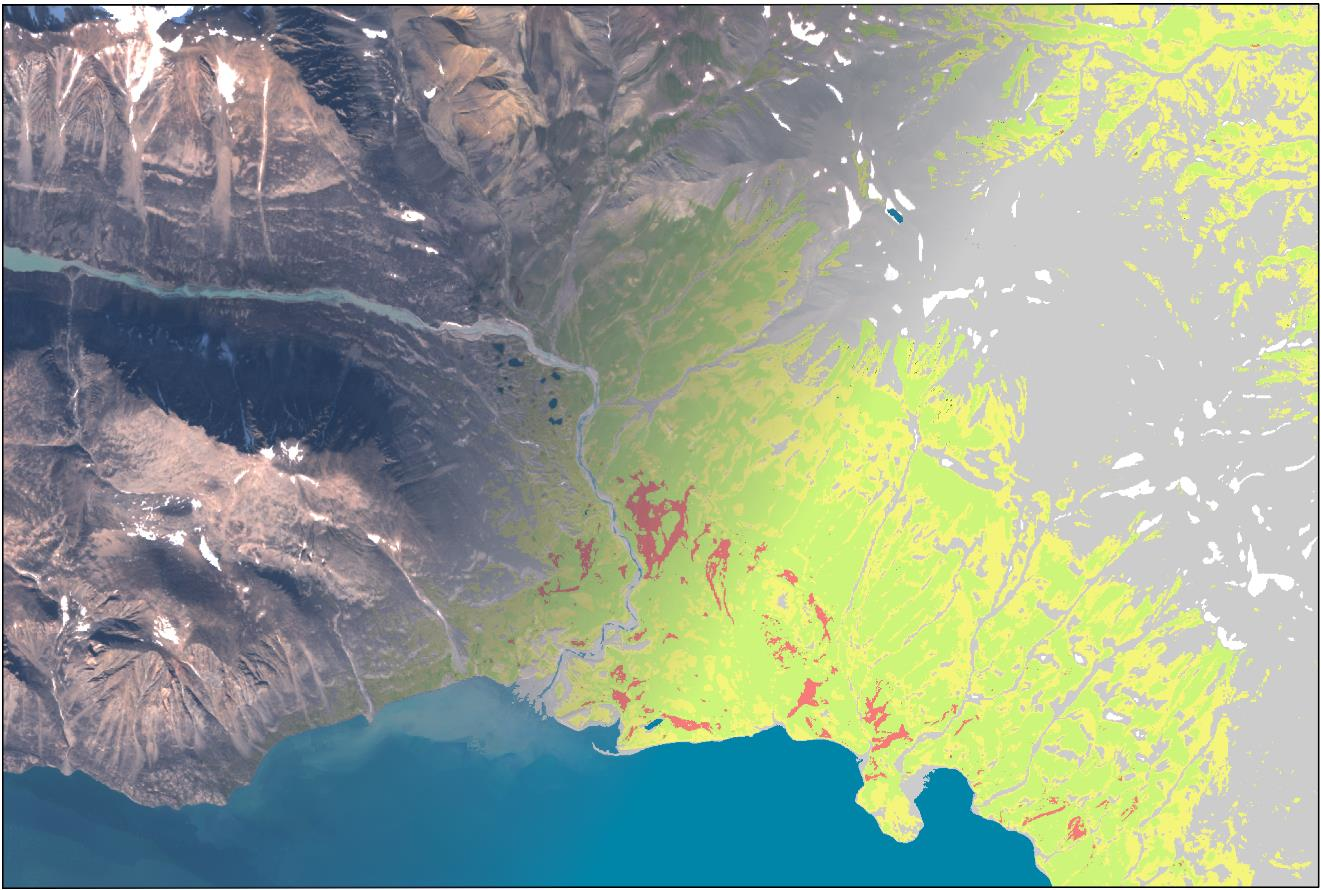
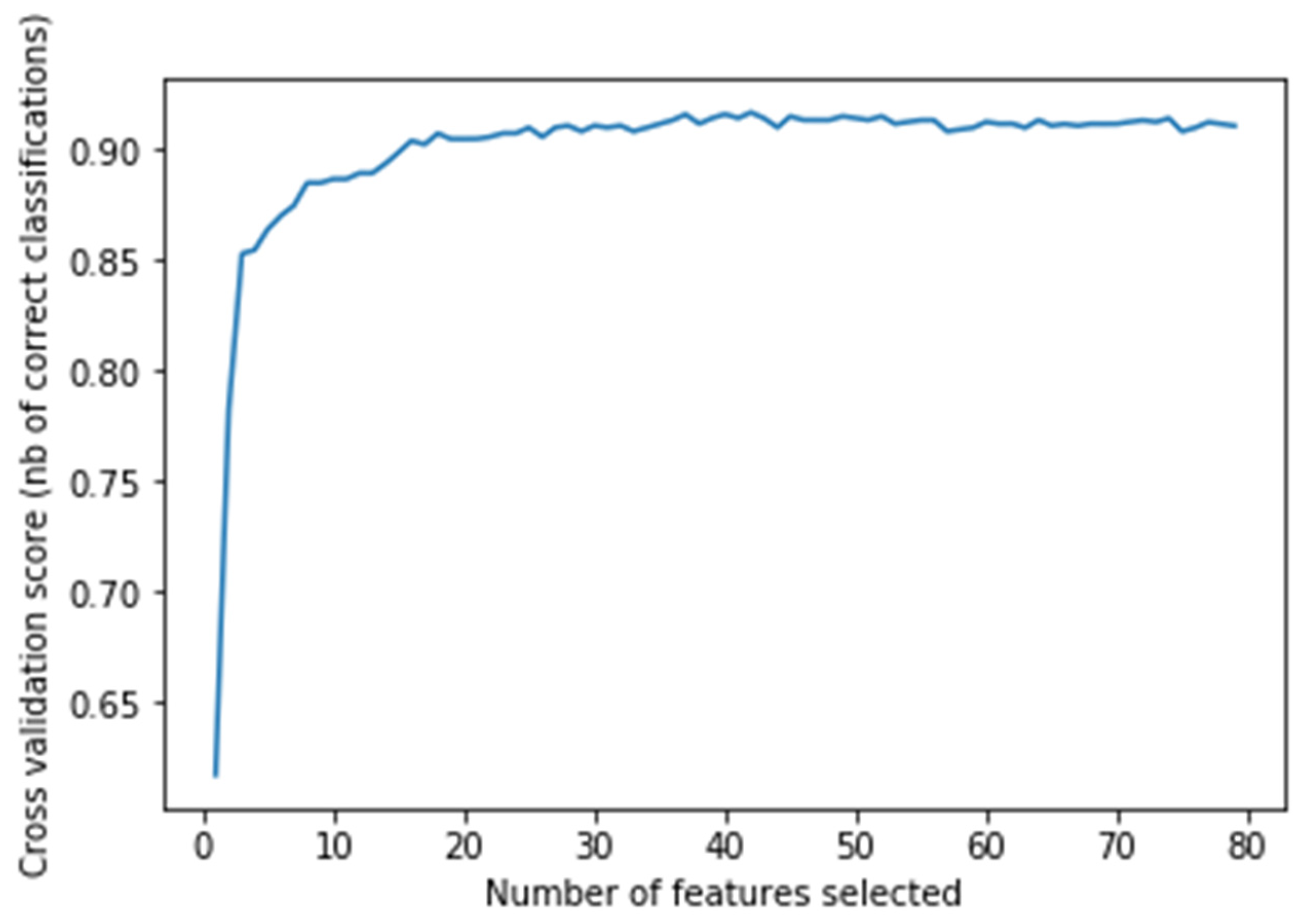
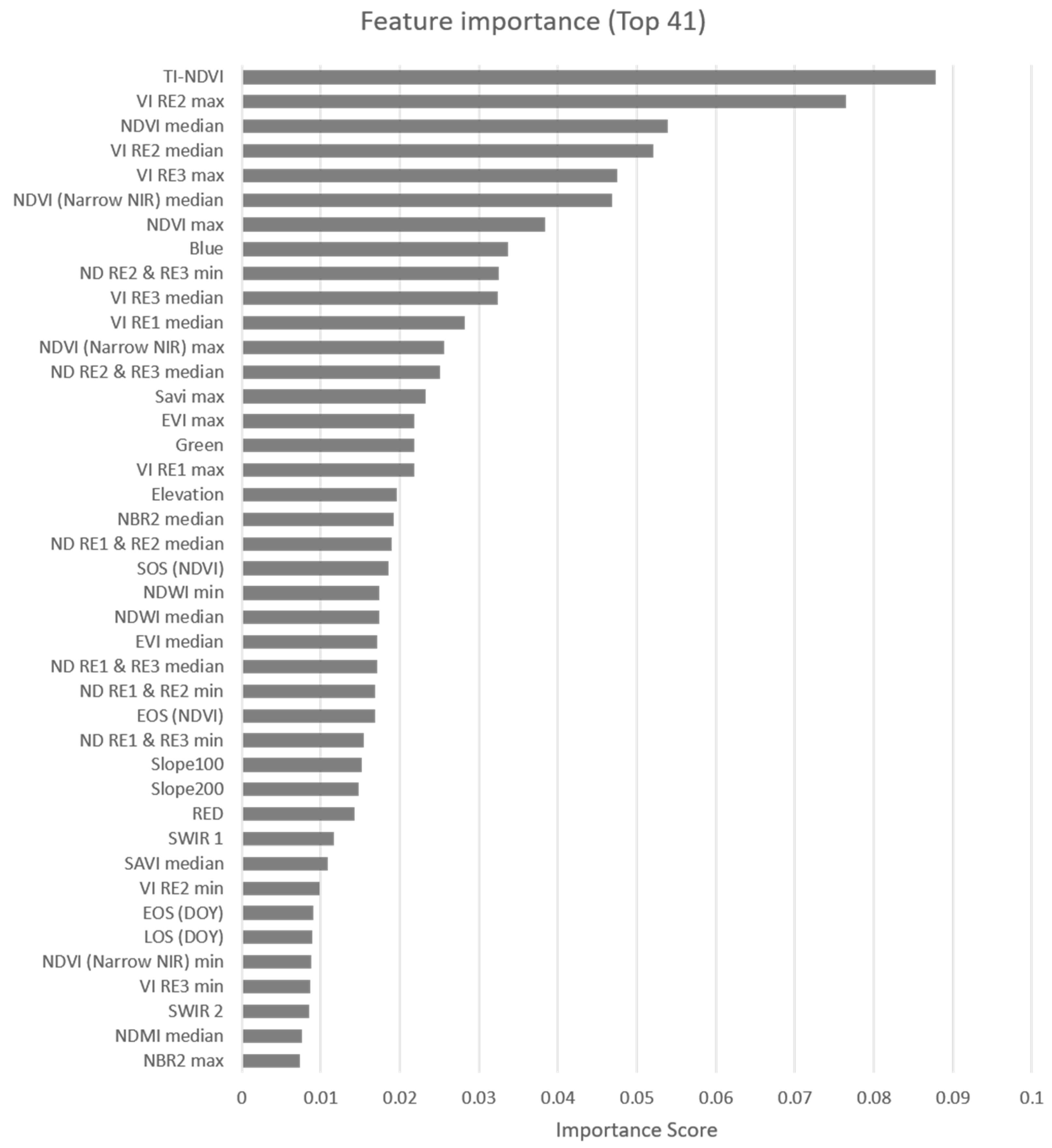
Accurate and precise (i.e., high spatial detail) land-cover mapping is pivotal for improved ecosystem modeling and GHG-related research in the highly heterogeneous Arctic region. The classification framework developed in Google Earth Engine was able to produce high-resolution land cover maps (10 m resolution) covering different climatic and phenological conditions in Greenland. Based on 41 extracted features (vegetation indices, spectral reflectance, and phenology metrics) derived from Sentinel-2 data during 2019 and a DEM, the RF classifier was able to reach a high level of accuracy (OA of 91.8%) when compared against a total of 1164 GRD points. The use of vegetation phenology features derived from Sentinel-2 data, as a means to restrict observations for which features are extracted, was found to be a suitable way to standardize the multi-temporal dataset used. This made the classification framework able to deal with the challenge of area-specific differences in phenology and image availability.
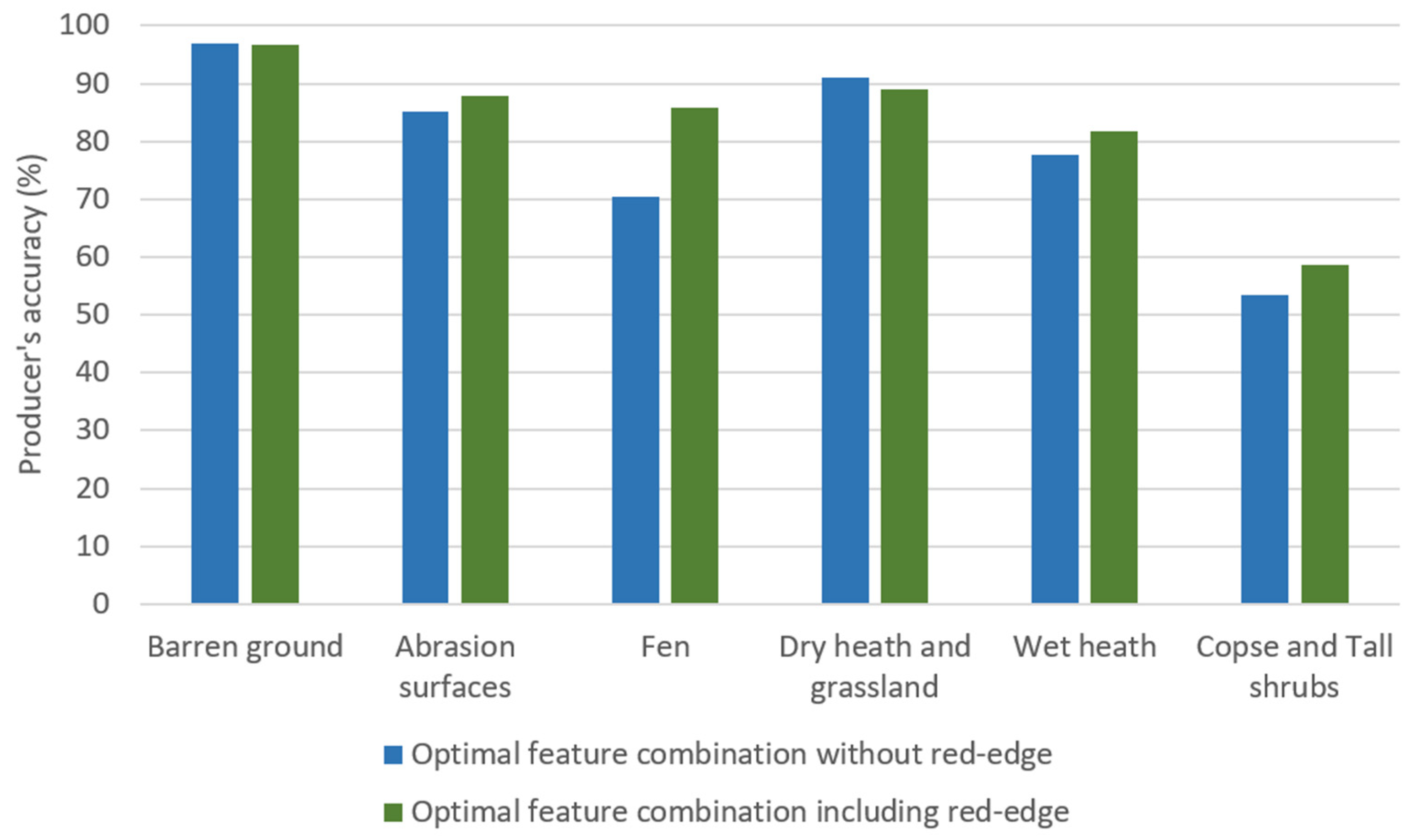
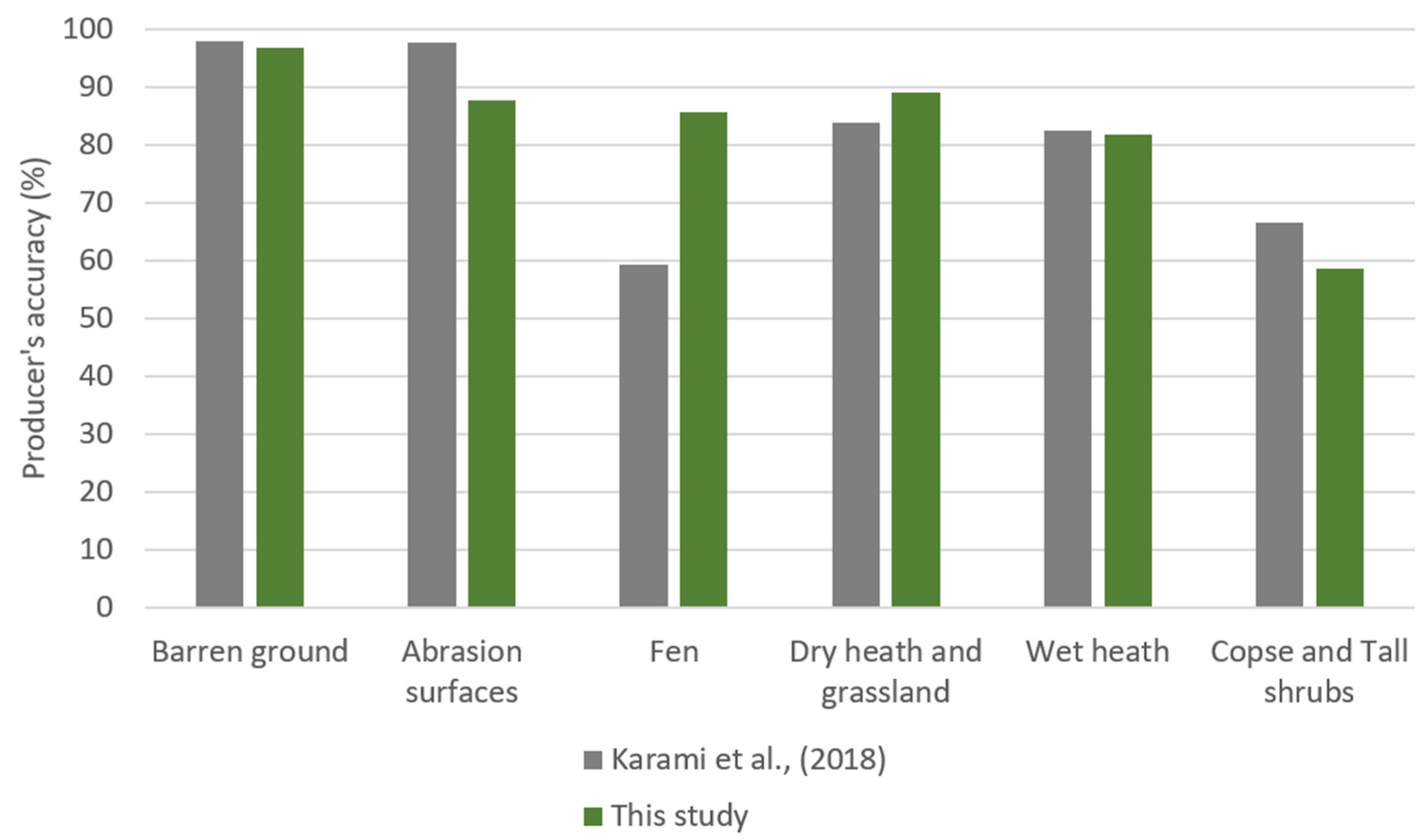
Both phenology and red-edge features derived from Sentinel-2 imagery were found to be of high importance for the classification of land cover in Greenland and increased classification performance was especially observed for the fen class as compared to previous studies based on Landsat data. The overall accuracy of the current classification was found to be at the same level as compared to state-of-the-art mapping of the region, yet the improved spatial resolution (of almost one order of magnitude) of the current study offers considerable advantages for future applications within up-scaling of ground-based climate change ecosystem research.
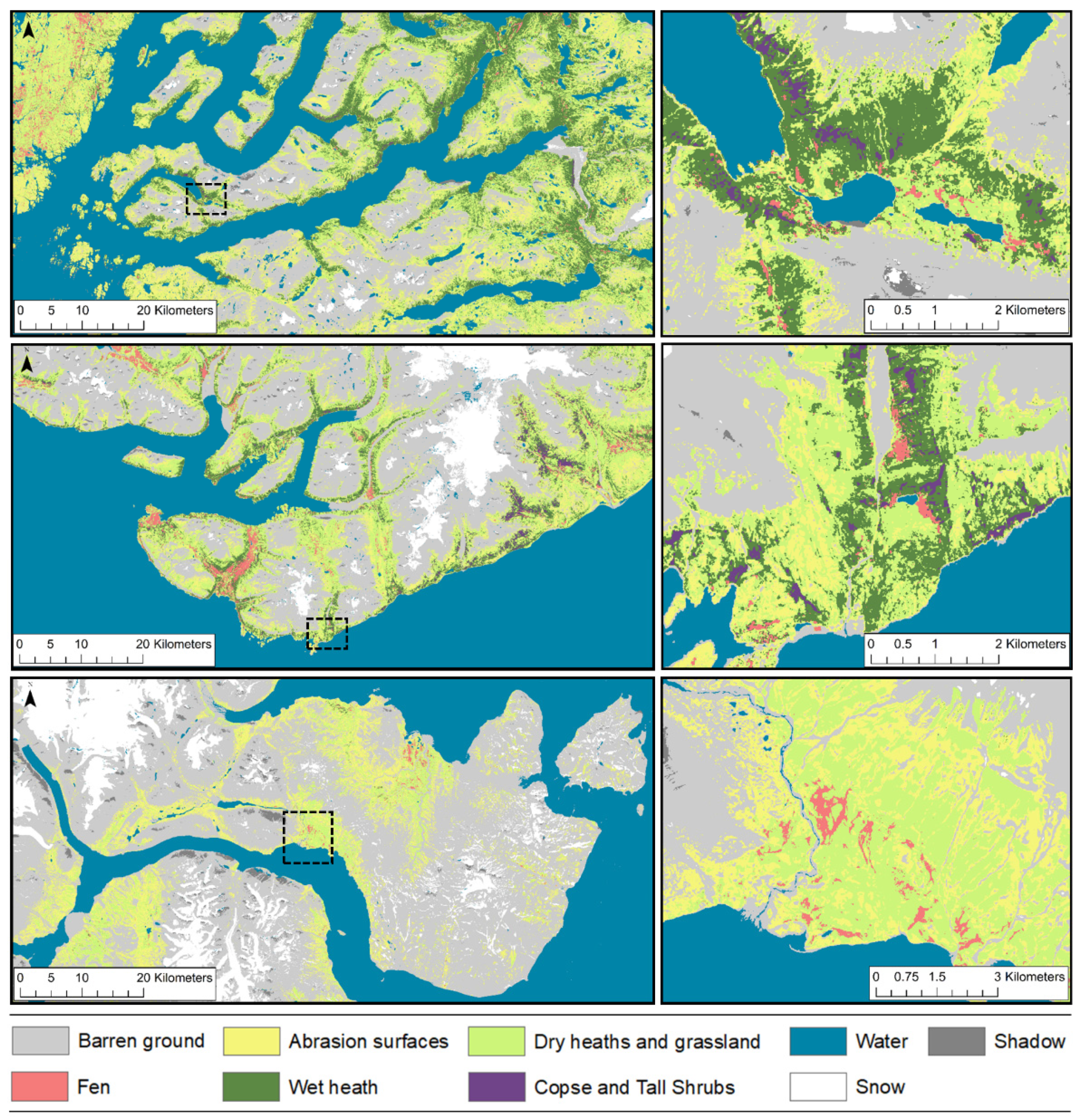
The final classified maps revealed a different distribution of land cover classes across the three case areas. Given the variability in climate and thereby vegetation structure and functioning between the three case areas, it is expected that the proposed framework can be used in extrapolating to other Arctic areas than the ones covered in the present study. The cloud-based framework is scalable and can be easily adapted to classify larger parts (potentially full coverage) of Greenland with a spatial resolution of 10 m. For a wall-to-wall classification of the entire ice-free Greenland, it is, however, important to consider to what extent the land cover classes operated (as defined by the training data set) represent the remaining land cover in Greenland.

Supplementary Materials

The following are available online at https://0-www-mdpi-com.brum.beds.ac.uk/article/10.3390/rs13183559/s1, Figures S1–S9 and Tables S1–S3.

Author Contributions

D.A.R. conceived, designed and performed the analyses. D.A.R. and M.K. were responsible for the collection and curation of GRD. D.A.R. and R.F. wrote the paper. All authors have read and agreed to the published version of the manuscript.

Funding

R.F. acknowledge support by the Villum Foundation through the project ‘Deep Learning and Remote Sensing for Unlocking Global Ecosystem Resource Dynamics’ (DeReEco).

Data Availability Statement

Not applicable.

Acknowledgments

Some parts of the ground reference data and drone images used in this study has been obtained as part of the Greenland Ecosystem Monitoring (https://g-e-m.dk/, accessed on 20 April 2021), for which the authors would like to express their gratitude.

Conflicts of Interest

The authors declare no conflict of interest.

References

  1. Shukla, P.; Skea, J.; Calvo Buendia, E.; Masson-Delmotte, V.; Pörtner, H.; Roberts, D.; Zhai, P.; Slade, R.; Connors, S.; Van Diemen, R. IPCC, 2019: Climate Change and Land: An IPCC Special Report on Climate Change, Desertification, Land Degradation, Sustainable Land Management, Food Security, and Greenhouse Gas Fluxes in Terrestrial Ecosystems; IPCC: Geneva, Switzerland, 2019. [Google Scholar]
  2. Christensen, T.R.; Friborg, T.; Sommerkorn, M.; Kaplan, J.; Illeris, L.; Soegaard, H.; Nordstroem, C.; Jonasson, S. Trace gas exchange in a high-Arctic valley: 1. Variationsin CO2 and CH4 Flux between tundra vegetation types. Glob. Biogeochem. Cycles 2000, 14, 701–713. [Google Scholar] [CrossRef]
  3. D’Imperio, L.; Nielsen, C.S.; Westergaard-Nielsen, A.; Michelsen, A.; Elberling, B. Methane oxidation in contrasting soil types: Responses to experimental warming with implication for landscape-integrated CH4 budget. Glob. Chang. Biol. 2017, 23, 966–976. [Google Scholar] [CrossRef] [Green Version]
  4. Juncher Jørgensen, C.; Lund Johansen, K.M.; Westergaard-Nielsen, A.; Elberling, B. Net regional methane sink in High Arctic soils of northeast Greenland. Nat. Geosci. 2014, 8, 20–23. [Google Scholar] [CrossRef]
  5. Blok, D.; Heijmans, M.M.P.D.; Schaepman-Strub, G.; Kononov, A.V.; Maximov, T.C.; Berendse, F. Shrub expansion may reduce summer permafrost thaw in Siberian tundra. Glob. Chang. Biol. 2010, 16, 1296–1305. [Google Scholar] [CrossRef]
  6. Juszak, I.; Erb, A.M.; Maximov, T.C.; Schaepman-Strub, G. Arctic shrub effects on NDVI, summer albedo and soil shading. Remote Sens. Environ. 2014, 153, 79–89. [Google Scholar] [CrossRef] [Green Version]
  7. Bartsch, A.; Höfler, A.; Kroisleitner, C.; Trofaier, A. Land cover mapping in northern high latitude permafrost regions with satellite data: Achievements and remaining challenges. Remote Sens. 2016, 8, 979. [Google Scholar] [CrossRef] [Green Version]
  8. Westermann, S.; Elberling, B.; Højlund Pedersen, S.; Stendel, M.; Hansen, B.U.; Liston, G.E. Future permafrost conditions along environmental gradients in Zackenberg, Greenland. Cryosphere 2015, 9, 719–735. [Google Scholar] [CrossRef] [Green Version]
  9. Azzari, G.; Lobell, D.B. Landsat-based classification in the cloud: An opportunity for a paradigm shift in land cover monitoring. Remote Sens. Environ. 2017, 202, 64–74. [Google Scholar] [CrossRef]
  10. Kumar, L.; Mutanga, O. Google Earth Engine applications since inception: Usage, trends, and potential. Remote Sens. 2018, 10, 1509. [Google Scholar] [CrossRef] [Green Version]
  11. Pekel, J.F.; Cottam, A.; Gorelick, N.; Belward, A.S. High-resolution mapping of global surface water and its long-term changes. Nature 2016, 540, 418–422. [Google Scholar] [CrossRef]
  12. Gorelick, N.; Hancher, M.; Dixon, M.; Ilyushchenko, S.; Thau, D.; Moore, R. Google Earth Engine: Planetary-scale geospatial analysis for everyone. Remote Sens. Environ. 2017, 202, 18–27. [Google Scholar] [CrossRef]
  13. Carrasco, L.; O’Neil, A.; Morton, R.; Rowland, C. Evaluating combinations of temporally aggregated Sentinel-1, Sentinel-2 and Landsat 8 for land cover mapping with Google Earth Engine. Remote Sens. 2019, 11, 288. [Google Scholar] [CrossRef] [Green Version]
  14. Poortinga, A.; Clinton, N.; Saah, D.; Cutter, P.; Chishtie, F.; Markert, K.; Anderson, E.; Troy, A.; Fenn, M.; Tran, L.; et al. An operational Before-After-Control-Impact (BACI) designed platform for vegetation monitoring at planetary scale. Remote Sens. 2018, 10, 760. [Google Scholar] [CrossRef] [Green Version]
  15. Fred, J.A.D. Vegetation classification in Greenland. J. Veg. Sci. 1994, 5, 781–790. [Google Scholar] [CrossRef]
  16. Raynolds, M.K.; Walker, D.A.; Balser, A.; Bay, C.; Campbell, M.; Cherosov, M.M.; Daniëls, F.J.A.; Eidesen, P.B.; Ermokhina, K.A.; Frost, G.V.; et al. A raster version of the Circumpolar Arctic Vegetation Map (CAVM). Remote Sens. Environ. 2019, 232, 111297. [Google Scholar] [CrossRef]
  17. Walker, D.A.; Daniëls, F.J.A.; Matveyeva, N.V.; Šibík, J.; Walker, M.D.; Breen, A.L.; Druckenmiller, L.A.; Raynolds, M.K.; Bültmann, H.; Hennekens, S.; et al. Circumpolar Arctic vegetation classification. Phytocoenologia 2018, 48, 181–201. [Google Scholar] [CrossRef]
  18. Karami, M.; Westergaard-Nielsen, A.; Normand, S.; Treier, U.A.; Elberling, B.; Hansen, B.U. A phenology-based approach to the classification of Arctic tundra ecosystems in Greenland. ISPRS J. Photogramm. Remote Sens. 2018, 146, 518–529. [Google Scholar] [CrossRef]
  19. Jensen, J.R. Remote Sensing of the Environment: An Earth Resource Perspective, 2nd ed.; Pearson Education: Delhi, India, 2009. [Google Scholar]
  20. Hennessy, A.; Clarke, K.; Lewis, M. Hyperspectral classification of plants: A review of waveband selection generalisability. Remote Sens. 2020, 12, 113. [Google Scholar] [CrossRef] [Green Version]
  21. Raynolds, M.K.; Walker, D.A.; Epstein, H.E.; Pinzon, J.E.; Tucker, C.J. A new estimate of tundra-biome phytomass from trans-Arctic field data and AVHRR NDVI. Remote Sens. Lett. 2011, 3, 403–411. [Google Scholar] [CrossRef]
  22. Stow, D.A.; Hope, A.; McGuire, D.; Verbyla, D.; Gamon, J.; Huemmrich, F.; Houston, S.; Racine, C.; Sturm, M.; Tape, K.; et al. Remote sensing of vegetation and land-cover change in Arctic Tundra Ecosystems. Remote Sens. Environ. 2004, 89, 281–308. [Google Scholar] [CrossRef] [Green Version]
  23. Eklundh, L.; Jönsson, P. TIMESAT: A software package for time-series processing and assessment of vegetation dynamics. In Remote Sensing Time Series; Springer: Cham, Switzerland, 2015; pp. 141–158. [Google Scholar]
  24. Khatami, R.; Mountrakis, G.; Stehman, S.V. A meta-analysis of remote sensing research on supervised pixel-based land-cover image classification processes: General guidelines for practitioners and future research. Remote Sens. Environ. 2016, 177, 89–100. [Google Scholar] [CrossRef] [Green Version]
  25. Feng, M.; Sexton, J.O.; Channan, S.; Townshend, J.R. A global, high-resolution (30-m) inland water body dataset for 2000: First results of a topographic–spectral classification algorithm. Int. J. Digit. Earth 2015, 9, 113–133. [Google Scholar] [CrossRef] [Green Version]
  26. Verpoorter, C.; Kutser, T.; Tranvik, L. Automated mapping of water bodies using Landsat multispectral data. Limnol. Oceanogr. Methods 2012, 10, 1037–1050. [Google Scholar] [CrossRef]
  27. Feyisa, G.L.; Meilby, H.; Fensholt, R.; Proud, S.R. Automated water extraction index: A new technique for surface water mapping using Landsat imagery. Remote Sens. Environ. 2014, 140, 23–35. [Google Scholar] [CrossRef]
  28. Fisher, A.; Flood, N.; Danaher, T. Comparing Landsat water index methods for automated water classification in eastern Australia. Remote Sens. Environ. 2016, 175, 167–182. [Google Scholar] [CrossRef]
  29. Breiman, L. Random forests. Mach. Learn. 2001, 45, 5–32. [Google Scholar] [CrossRef] [Green Version]
  30. Christensen, T.R.; Topp-Jørgensen, E. Greenland Ecosystem Monitoring Strategy 2017–2021; DCE—Danish Centre for Environment and Energy, Aarhus University: Aarhus, Denmark, 2016; p. 44. [Google Scholar]
  31. Elberling, B.; Tamstorf, M.P.; Michelsen, A.; Arndal, M.F.; Sigsgaard, C.; Illeris, L.; Bay, C.; Hansen, B.U.; Christensen, T.R.; Hansen, E.S.; et al. Soil and plant community-characteristics and dynamics at Zackenberg. Adv. Ecol. Res. 2008, 40, 223–248. [Google Scholar]
  32. Karami, M.; Hansen, B.U.; Westergaard-Nielsen, A.; Abermann, J.; Lund, M.; Schmidt, N.M.; Elberling, B. Vegetation phenology gradients along the west and east coasts of Greenland from 2001 to 2015. Ambio 2017, 46, 94–105. [Google Scholar] [CrossRef] [Green Version]
  33. Drusch, M.; Del Bello, U.; Carlier, S.; Colin, O.; Fernandez, V.; Gascon, F.; Hoersch, B.; Isola, C.; Laberinti, P.; Martimort, P.; et al. Sentinel-2: ESA’s optical high-resolution mission for GMES operational services. Remote Sens. Environ. 2012, 120, 25–36. [Google Scholar] [CrossRef]
  34. Howat, I.M.; Negrete, A.; Smith, B.E. The Greenland Ice Mapping Project (GIMP) land classification and surface elevation data sets. Cryosphere 2014, 8, 1509–1518. [Google Scholar] [CrossRef] [Green Version]
  35. Hall, D.K.; Riggs, G.A.; Salomonson, V.V.; Barton, J.; Casey, K.; Chien, J.; DiGirolamo, N.; Klein, A.; Powell, H.; Tait, A. Algorithm Theoretical Basis Document (ATBD) for the MODIS Snow and Sea Ice-Mapping Algorithms. Nasa GSFC. 2001; p. 45. Available online: https://eospso.gsfc.nasa.gov/sites/default/files/atbd/atbd_mod10.pdf (accessed on 20 April 2021).
  36. McFeeters, S.K. The use of the normalized difference water index (NDWI) in the delineation of open water features. Int. J. Remote. Sens. 1996, 17, 1425–1432. [Google Scholar] [CrossRef]
  37. Rouse, J.W.; Haas, R.H.; Schell, J.A.; Deering, D.W.; Harlan, J.C. Monitoring the Vernal Advancement and Retrogradation (Green Wave Effect) of Natural Vegetation. NASA/GSFC Type III Final Report, Greenbelt, Md. 1974, p. 371. Available online: https://core.ac.uk/download/pdf/42887948.pdf (accessed on 23 April 2021).
  38. Fernández-Manso, A.; Fernández-Manso, O.; Quintano, C. SENTINEL-2A red-edge spectral indices suitability for discriminating burn severity. Int. J. Appl.Earth Obs. Geoinf. 2016, 50, 170–175. [Google Scholar] [CrossRef]
  39. Ji, L.; Zhang, L.; Wylie, B.K.; Rover, J. On the terminology of the spectral vegetation index (NIR − SWIR)/(NIR + SWIR). Int. J. Remote Sens. 2011, 32, 6901–6909. [Google Scholar] [CrossRef]
  40. Key, C.H.; Benson, N.C. Measuring and remote sensing of burn severity. In Proceedings of the Joint Fire Science Conference and Workshop, Boise, ID, USA, 15–17 June 1999; p. 284. [Google Scholar]
  41. Huete, A.; Didan, K.; van Leeuwen, W.; Vermote, E. Global-scale analysis of vegetation indices for moderate resolution monitoring of terrestrial vegetation. In Remote Sensing for Earth Science, Ocean, and Sea Ice Applications, Proceedings of the Remote Sensing, Florence, Italy, 20–24 September 1999; SPIE: Bellingham, WA, USA, 1999; Volume 3868, pp. 141–151. [Google Scholar] [CrossRef]
  42. Huete, A.R. A soil-adjusted vegetation index (SAVI). Remote Sens. Environ. 1988, 25, 295–309. [Google Scholar] [CrossRef]
  43. Boehmke, B.; Greenwell, B.M. Hands-on Machine Learning with R; CRC Press: Boca Raton, FL, USA, 2019. [Google Scholar]
  44. Belgiu, M.; Drăguţ, L. Random forest in remote sensing: A review of applications and future directions. ISPRS J. Photogramm. Remote Sens. 2016, 114, 24–31. [Google Scholar] [CrossRef]
  45. Olofsson, P.; Foody, G.M.; Herold, M.; Stehman, S.V.; Woodcock, C.E.; Wulder, M.A. Good practices for estimating area and assessing accuracy of land change. Remote Sens. Environ. 2014, 148, 42–57. [Google Scholar] [CrossRef]
  46. Olofsson, P.; Foody, G.M.; Stehman, S.V.; Woodcock, C.E. Making better use of accuracy data in land change studies: Estimating accuracy and area and quantifying uncertainty using stratified estimation. Remote Sens. Environ. 2013, 129, 122–131. [Google Scholar] [CrossRef]
  47. Foody, G.M. Thematic map comparison: Evaluating the statistical significance of differences in classification accuracy. Photogramm. Eng. Remote Sens. 2004, 70, 627–633. [Google Scholar] [CrossRef]
  48. Prishchepov, A.V.; Radeloff, V.C.; Dubinin, M.; Alcantara, C. The effect of Landsat ETM/ETM plus image acquisition dates on the detection of agricultural land abandonment in Eastern Europe. Remote Sensi. Environ. 2012, 126, 195–209. [Google Scholar] [CrossRef]
  49. Acharya, T.D.; Subedi, A.; Lee, D.H. Evaluation of water indices for surface water extraction in a Landsat 8 scene of Nepal. Sensors 2018, 18, 2580. [Google Scholar] [CrossRef] [Green Version]
  50. Donchyts, G.; van de Giesen, N.; Gorelick, N. Reconstruction of reservoir and lake surface area dynamics from optical and SAR satellite imagery. In Proceedings of the International Workshop on the Analysis of Multitemporal Remote Sensing Images, Bruges, Belgium, 27–29 June 2017. [Google Scholar]
  51. Ji, L.; Zhang, L.; Wylie, B. Analysis of dynamic thresholds for the normalized difference water index. Photogramm. Eng. Remote Sens. 2009, 75, 1307–1317. [Google Scholar] [CrossRef]
  52. Jönsson, P.; Eklundh, L. TIMESAT—A program for analyzing time-series of satellite sensor data. Comput. Geosci. 2004, 30, 833–845. [Google Scholar] [CrossRef] [Green Version]
  53. Jung, M.; Chang, E. NDVI-based land-cover change detection using harmonic analysis. Int. J. Remote Sens. 2015, 36, 1097–1113. [Google Scholar] [CrossRef]
  54. Yan, E.; Wang, G.; Lin, H.; Xia, C.; Sun, H. Phenology-based classification of vegetation cover types in Northeast China using MODIS NDVI and EVI time series. Int. J. Remote Sens. 2015, 36, 489–512. [Google Scholar] [CrossRef]
  55. Forkuor, G.; Dimobe, K.; Serme, I.; Tondoh, J.E. Landsat-8 vs. Sentinel-2: Examining the added value of sentinel-2’s red-edge bands to land-use and land-cover mapping in Burkina Faso. GISci. Remote Sens. 2017, 55, 331–354. [Google Scholar] [CrossRef]
  56. Sun, L.; Chen, J.; Guo, S.; Deng, X.; Han, Y. Integration of time series Sentinel-1 and Sentinel-2 imagery for crop type mapping over oasis agricultural areas. Remote Sens. 2020, 12, 158. [Google Scholar] [CrossRef] [Green Version]
  57. Fletcher, K. SENTINEL 2: ESA’s Optical High-Resolution Mission for GMES Operational Services; European Space Agency: Paris, France, 2012. [Google Scholar]
  58. Hirayama, H.; Sharma, R.C.; Tomita, M.; Hara, K. Evaluating multiple classifier system for the reduction of salt-and-pepper noise in the classification of very-high-resolution satellite images. Int. J. Remote Sens. 2019, 40, 2542–2557. [Google Scholar] [CrossRef]
Figure 1. Location of the three study sites.
Remotesensing 13 03559 g001
Figure 2. Overview of the workflow from pre-processing to land-cover classification. The green boxes illustrate the final results.
Remotesensing 13 03559 g002
Figure 3. Cross validation (CV) scores in relation to the number of features included in the RF classifier.
Remotesensing 13 03559 g003
Figure 4. The ranking and importance score of the top 41 features used in the RF classifier.
Remotesensing 13 03559 g004
Figure 5. Final classified land-cover maps, Kobbefjord (upper), Disko (middle), and Zackenberg (lower). The right part of the map is a zoom-in of the dashed square in the full extent map.
Remotesensing 13 03559 g005
Figure 6. Comparison of the producer’s accuracy, after proportion adjustment, for the two subsets of optimal feature combination, with and without red-edge.
Remotesensing 13 03559 g006
Figure 7. (a) Boxplot of the extracted maximum values of VI RE2 throughout the growing season 2019, based on the 1164 GRD points. Number of GRD for each class is shown next to each class in the legend. (b) Median values of VI RE2 (left) and NDMI (right) for the 2019 growing season in a subset from Kobbefjord. Middle: Drone image from Kobbefjord. The image subset includes all six land cover classes included in the RF classifier to demonstrate the feature values in a heterogeneous area. The polygon illustrates the Kobbefjord Fen site, where methane measurements are conducted seasonally.
Remotesensing 13 03559 g007
Figure 8. Comparison of producer’s accuracy, after proportion adjustment, in this study as compared to Karami et al. [18].
Remotesensing 13 03559 g008
Table 1. Key climatic parameters for Kobbefjord, Disko, and Zackenberg [30].
SiteKobbefjordDiskoZackenberg
Climate zoneLow ArcticLow/High ArcticHigh Arctic
Mean annual temperature (°C)−0.9−3.2−9.2
Total annual precipitation (mm)782436200
Sea iceYesYesYes
PermafrostNoneDiscontinuousContinuous
Table 2. Description of surface classes according to Karami et al. [18].
Surface ClassCharacteristics
1.Barren groundNot covered by vegetation during the growing season; Mostly rocks or wind-blown surfaces in high elevations
2.Abrasion surfacesReceives low amount of snow in the winter; dry with very low vegetation activity during the growing season; Very sparse dryas and/or grasses
3.FenWater logged areas located in landscape depressions; covered with grasses and mosses
4.Dry heath and grasslandsBetula and Vaccinum; Almost no Salix; Relatively low amount of snow during winter, and therefore receive low amount of melt water in the growing season
5.Wet heathA mix of Betula, Vaccinum, Salix, and Empetrum; Receive relatively more amount of snow in the winter compared with dry heath and are therefore more wet in the growing season; Not higher than 40 cm in height
6.Copse and Tall shrubsMostly Salix and Betula. Taller than 40 cm; Receive fair amount of snow during winter and are wet during the growing season
Table 3. Number of ground reference data points for each of the three study sites.
KobbefjordDiskoZackenbergTotal GRD
Barren ground7081116267
Abrasion surfaces392380142
Fen839111203
Dry heaths and grasslands5944143246
Wet heath163315199
Copse and Tall Shrubs57482107
Total GRD4712364571164
Table 4. Overview of indices used.
Spectral IndexFormulationReference
NDVI (Narrow NIR) ( B 8 A     B 4 )   /   ( B 8 A + B 4 ) [37]
VI RE1 ( B 8 A     B 5 )   /   ( B 8 A + B 5 ) [38]
VI RE2 ( B 8 A     B 6 )   /   ( B 8 A + B 6 ) [38]
VI RE3 ( B 8 A     B 7 )   /   ( B 8 A + B 7 ) [38]
NDMI ( B 8 A     B 11 )   /   ( B 8 A + B 11 ) [39]
NBR ( B 8 A     B 12 )   /   ( B 8 A + B 12 ) [40]
NBR2 ( B 11     B 12 )   /   ( B 11 + B 12 ) [40]
ND RE1 & RE2 ( B 5     B 6 )   /   ( B 5 + B 6 ) [38]
ND RE1 & RE3 ( B 5     B 7 )   /   ( B 5 + B 7 ) [38]
ND RE2 & RE3 ( B 6     B 7 )   /   ( B 6 + B 7 ) [38]
EVI ( B 8     B 4 ) / ( B 8 + 6     B 4     7.5     B 2 ) [41]
SAVI 1.5     ( ( B 8     B 4 ) / ( B 8 + B 4 + 0.5 ) [42]
NDWI ( B 3     B 8 ) / ( B 3 + B 8 ) [36]
Table 5. Distribution (error adjusted estimates) of the terrestrial land-cover classes for the case areas, with a 95% confidence interval.
Kobbefjord (%)Disko (%)Zackenberg (%)
Barren ground31.7 (±1.2)50.6 (±1.2)75.0 (±1.7)
Abrasion surfaces19.3 (±1.6)11.8 (±1.3)15.0 (±1.7)
Fen2.1 (±0.4)3.1 (±0.3)0.4 (±0.1)
Dry heaths and grassland29.2 (±1.6)23.8 (±1.2)8.6 (±1.0)
Wet heath16.7 (±1.2)9.0 (±0.9)0.9 (±0.4)
Copse and Tall Shrubs0.9 (±0.5)1.7 (±0.3)<0.1 (±0.1)
Table 6. Confusion matrix and accuracy assessment of vegetation classification based on a 10-fold cross-validation.
Reference
Barren groundAbrasion surfacesFenDry heaths and grasslandWet heathCopse and Tall ShrubsTotalProd. acc. after proportion adjustment (%)User’s acc. after proportion adjustment (%)
PredictedBarren ground2516010025896.897.3
Abrasion surfaces151270133015887.880.4
Fen1019914120685.896.6
Dry heaths and grassland08221515224289.088.8
Wet heath01215171419381.888.6
Copse and Tall Shrubs0001610010758.693.5
Total2671422032461991071164
Area-weighted OA 91.8
Publisher’s Note: MDPI stays neutral with regard to jurisdictional claims in published maps and institutional affiliations.

