
Horizon Picking from SBP Images Using Physicals-Combined Deep Learning


1
School of Geodesy and Geomatics, Wuhan University, Wuhan 430079, China
2
Institute of Marine Science and Technology, Wuhan University, Wuhan 430079, China
*
Author to whom correspondence should be addressed.
Remote Sens. 2021, 13(18), 3565; https://0-doi-org.brum.beds.ac.uk/10.3390/rs13183565
Submission received: 8 July 2021
/
Revised: 25 August 2021
/
Accepted: 31 August 2021
/
Published: 8 September 2021
(This article belongs to the Special Issue Deep Learning for Radar and Sonar Image Processing)
Abstract
:Horizon picking from sub-bottom profiler (SBP) images has great significance in marine shallow strata studies. However, the mainstream automatic picking methods cannot handle multiples well, and there is a need to set a group of parameters manually. Considering the constant increase in the amount of SBP data and the high efficiency of deep learning (DL), we proposed a physicals-combined DL method to pick the horizons from SBP images. We adopted the DeeplabV3+ net to extract the horizons and multiples from SBP images. We generated a training dataset from the Jiaozhou Bay survey (Shandong, China) and the Zhujiang estuary survey (Guangzhou, China) to increase the applicability of the trained model. After the DL processing, we proposed a simulated Radon transform method to eliminate the surface-related multiples from the prediction by combining the designed pseudo-Radon transform and correlation analysis. We verified the proposed method using actual data (not involved in the training dataset) from Jiaozhou Bay and Zhujiang estuary. The positions of picked horizons are accurate, and multiples are suppressed.
1. Introduction
Obtaining sub-bottom structures using acoustic equipment is one of the main components of marine shallow strata study [1]. It plays a significant role in marine mineral discovery, marine oil/gas exploration [2,3] and marine infrastructure construction [4], and so on. As a prevalent acoustic means of obtaining sub-bottom structure, the sub-bottom profiler (SBP) provides fundamental information for sub-bottom exploration and mining operations.
SBP is a type of sonar system that is designed to produce 2-dimensional stratigraphic cross-sectional images called SBP images [5]. Generally, the transducer of an SBP system converts the control signals to acoustic pulses (100 Hz–10 kHz) and emits the pulses towards the seafloor. After the pulse encounters the sediment, acoustic energy reflected from the horizons is received by the transducer and recorded as a time series called “ping”. Finally, the ping is converted to a series of gray values, and all the adjacent pings compose an SBP image. Therefore, SBP has the advantage of displaying different horizons and collecting information about acoustic sound propagation at low frequencies. The extracted horizons on SBP images allow the interpreter to identify and correlate lithologic interfaces and sequence stratigraphic boundaries [6,7,8]. Horizon picking is thus a key step directly affecting the accuracy of sediment classification and geological structure determination.
Many researchers have made their efforts in the field of horizon picking. From Bondár et al. [9] to Maroni et al. [10], traditional image processing methods were employed in horizon picking, like the edge detection method and multi-resolution analysis method. These methods provide a set of means to obtain horizons automatically and significantly reduce the manual workload. However, these methods all need to set intensity-related threshold parameters manually. Because the acoustic wave attenuates with the propagating distance increasing, lateral variations of overlying layer thickness produce gradual lateral changes in the intensities of reflections below this layer. The methods mentioned above may suffer challenges when the reflectors’ intensities change since a single intensity threshold cannot extract the horizons of a whole surveying line. In addition, faced with a complex distribution of geological structure, continuous horizons are always difficult to obtain when employing these methods [11].
To reduce the influence of changing intensities on reflections, multi-scale rotated Haar-like feature filtering was used by Fakiris et al. [12]. Thus, it is helpful in picking reflections with low intensities. Dossi et al. [13] and Forte et al. [14] applied an attribute-based auto-picking algorithm, which uses the cosine phase to enhance seismic reflections and obtain continuous horizons. Zhao et al. [15] introduced the concept of cosine phase and local phase into SBP horizon picking. Phase information is helpful for continuous horizon extraction since the phase can ignore the change in intensity of reflections and highlight all the reflections. Li et al. [16] modified the traditional Frangi filtering method and took the line-like and no-vertical structures of reflectors into consideration. Since line-like characteristics are independent of intensities, to some degree, continuous horizons can be obtained using this method. Although these methods can deal with intensity changes and obtain continuous horizons, a set of parameters should be set appropriately, such as the intensity threshold parameters and scale parameters. The performance of these methods depends on properly setting the parameters. In addition, these methods may fail when multiples exist. The essence of multiples is that the multiple reflections of the real horizon are superimposed on the wrong position of SBP images [17,18,19]. Most characteristics of multiples and horizons are the same [20,21]. Thus, multiples are usually removed before extracting the horizons. Predictive deconvolution is the most prevalent method of multiple suppression for SBP images [22]. The effects of this method, however, depend on its predictive step. An inappropriate step will lead to incomplete multiples elimination, which will directly bring errors to the next extraction for the horizons.
Considering the constant increase in the amount of SBP data and the shortcomings of the existed automatic picking methods, we propose a deep-learning (DL) based methodology to support interpreters in the horizon picking from SBP images. DL-based methods have been prevalently adopted to solve similar problems in other domains, such as image classification [23,24,25]. As a popular method of DL, a convolutional neural network (CNN) can learn abstract features from images and deal with various complex scenes [26,27]. Due to this ability, CNN has been successfully applied to recognize the targets from a complex image [27,28,29]. Therefore, we propose to utilize a kind of CNN, the DeeplabV3+ net [30], to realize horizon picking from an SBP image.
Because the morphological characteristics of horizons and multiples are similar in the CNN, it is difficult to distinguish the two. To solve this problem, we propose a multiple suppression method to eliminate the surface-related multiples from the CNN prediction. The multiple suppression method refers to the Radon transform in the multi-channel seismic investigation. Since the SBP survey belongs to one-channel investigations, we used a combination of the proposed pseudo-Radon transform and correlation analysis to achieve the same effect of the Radon transform. After horizons and multiples are distinguished, to avoid detail information loss, we conduct high-pass filtering at the multiples region and superimpose the filtered image and the image that only contains horizons.
The feasibility and efficiency of the proposed method are verified by two field surveys, Jiaozhou Bay survey (Shandong, China) and Zhujiang estuary survey (Guangzhou, China). We generated the training dataset from two regions to increase the applicability of the trained model. To evaluate the ability to suppress multiples, we compared the identified horizons and the effect on acoustic signals by the DL-based method and predictive deconvolution. The comparison indicates that our proposed method not only traces horizons accurately but also retains the details.
The structure of this paper is organized as follows. In the Methodology section, we describe the methodology, including SBP data preprocessing, training dataset generation, network architecture, training process, and multiple suppression. Next, we apply the method to datasets obtained from Jiaozhou Bay survey and Zhujiang estuary survey (see experiments and results). In the Discussion and Conclusions section, we discuss and summarize the results.
2. Materials and Methods
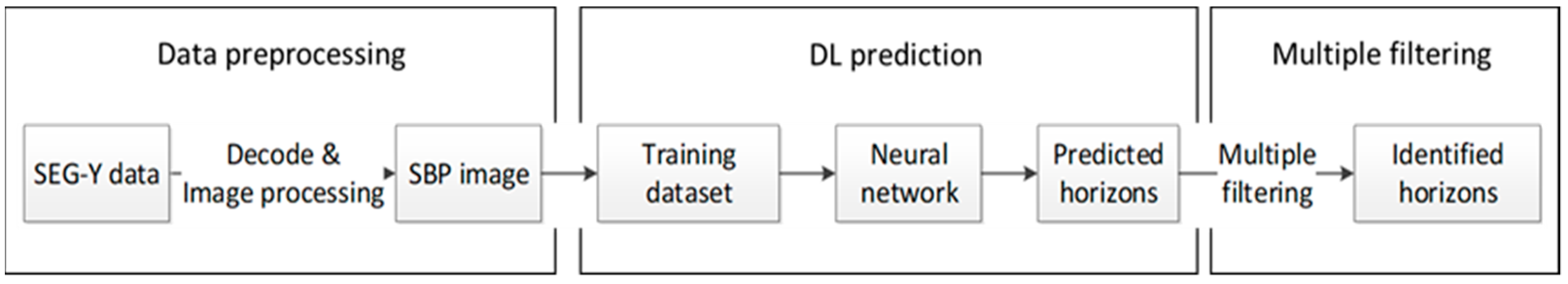
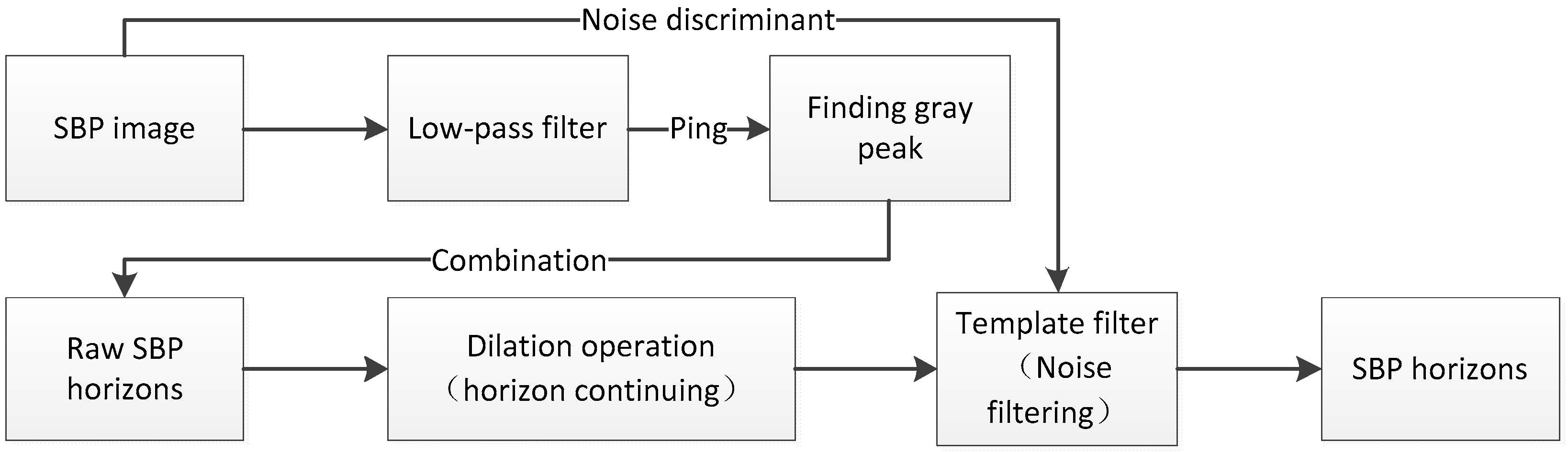
Different from existing methods, we extract the horizons and multiples first and then eliminate the multiples from the extractive. The workflow of the proposed horizon picking method is shown in Figure 1. The method is summarized by three major steps:
- Data preprocessing: convert SEG-Y data to SBP images;
- DL prediction: picking horizons (a crude result) from SBP images using the DL method;
- Multiple filtering: eliminate multiples from the picked horizons to obtain final horizons (a refined result). These three steps are elaborated below.
2.1. SBP Data Preprocessing
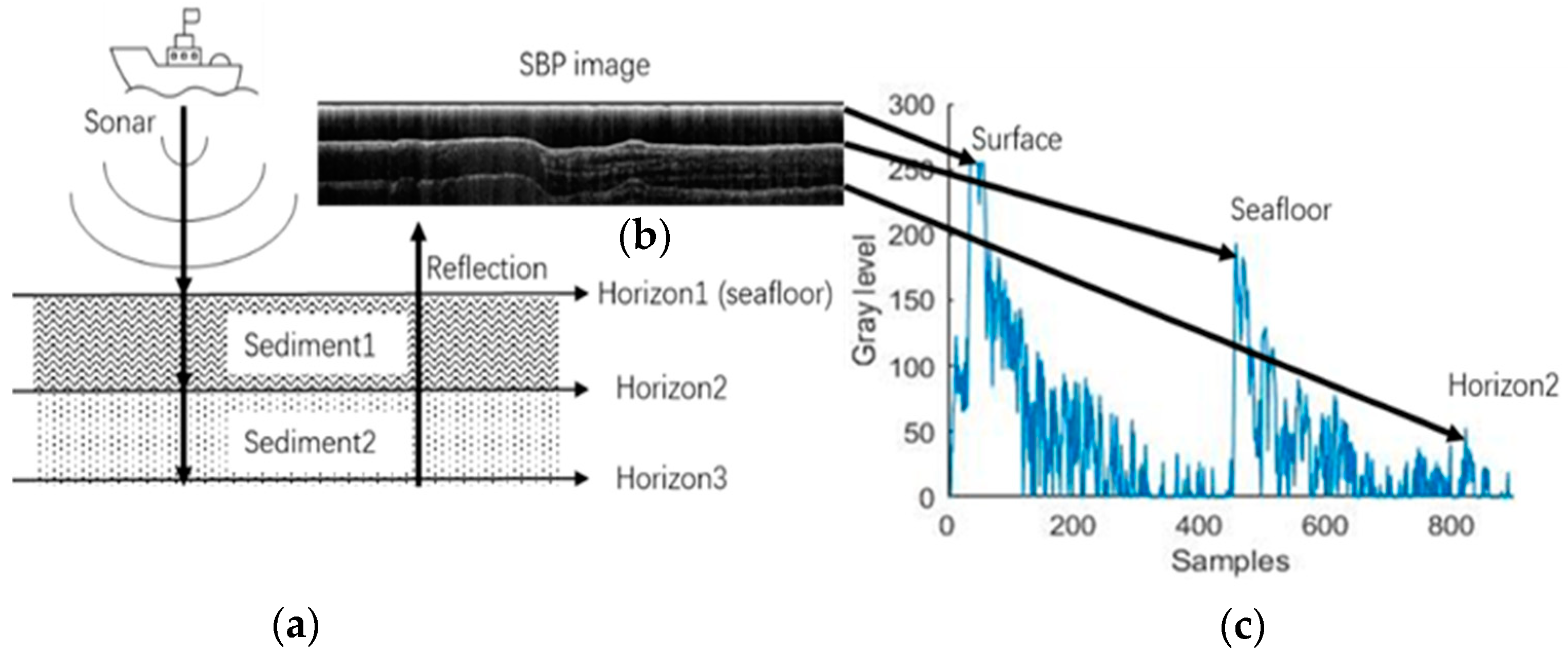
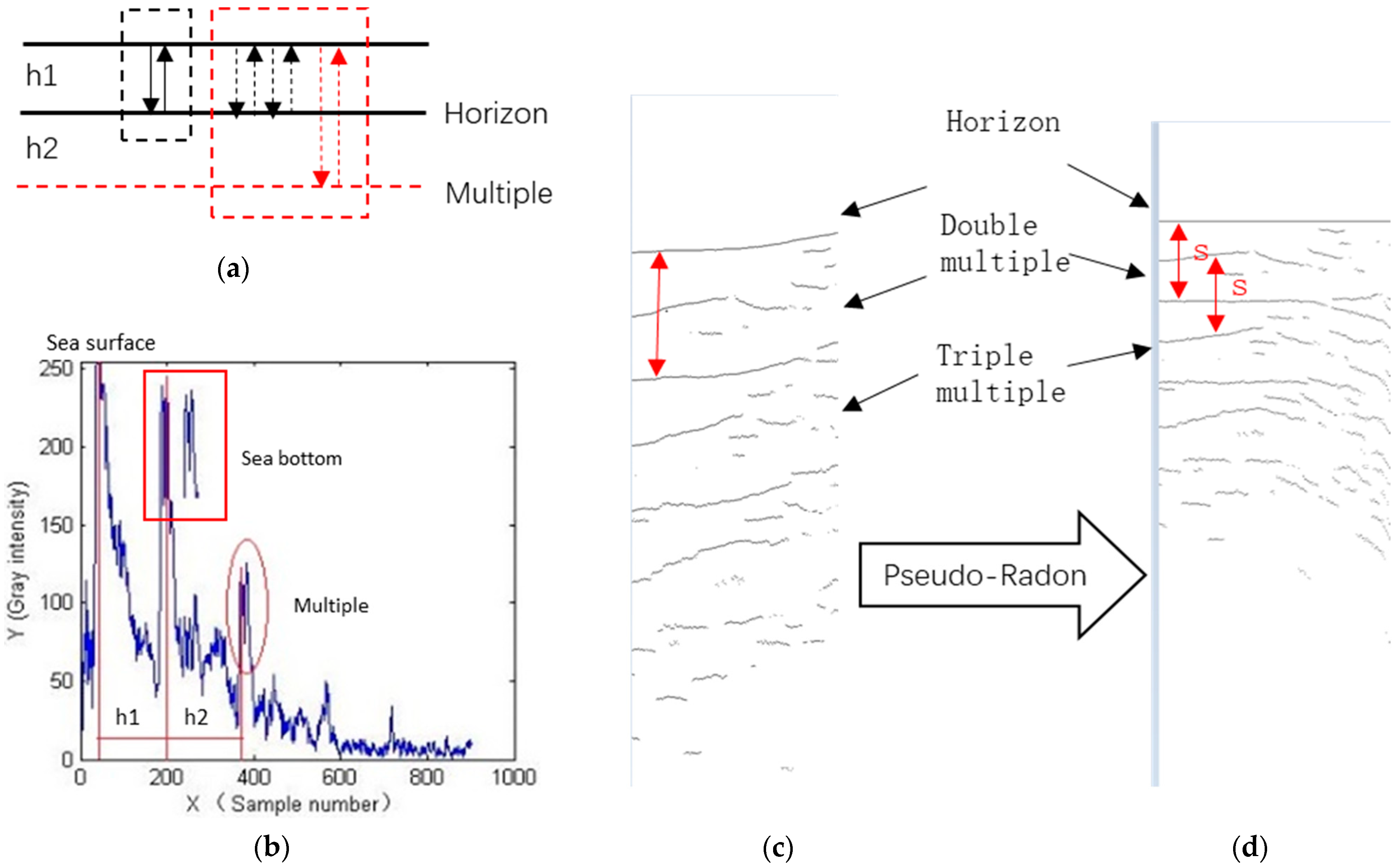
A general SBP survey is shown in Figure 2. SPB sonars emit pulses vertically towards the seafloor (Figure 2a). When the pulse encounters sediment, its reflected acoustic energy is received by the transducer as raw data files (SEG-Y data in this paper). Then the post-processor decodes the SEG-Y data and produces the SBP images (Figure 2b). The reflected energy is strong at the location of horizons, corresponding to the large gray values in SBP images (Figure 2c).
The accuracy of the training dataset is one of the decisive factors in determining the accuracy of the DL-based method. Since we generate a training dataset using the observed SBP data, we need to accurately locate the horizons in an SBP image to obtain correct labels. Thus, we utilized a series of image processing methods for the decoded data, including Hilbert transformation, image recovery, high-pass filtering, and gray equalization. These operations can improve the qualities of SBP images and the continuity of horizons.
2.2. DL-Based Identification
The DL approach for horizon picking can be simplified into four steps:
- 4.
- Generate training dataset and validation dataset in a 3:1 ratio;
- 5.
- Design a neural network and then use the training dataset to train the network;
- 6.
- Select a well-trained network according to the training loss, validation loss, and accuracy;
- 7.
- Once the network is trained, it will output horizons for any observed SBP images.
We will describe our proposed method in detail below according to these steps.
2.2.1. Training Dataset Generation
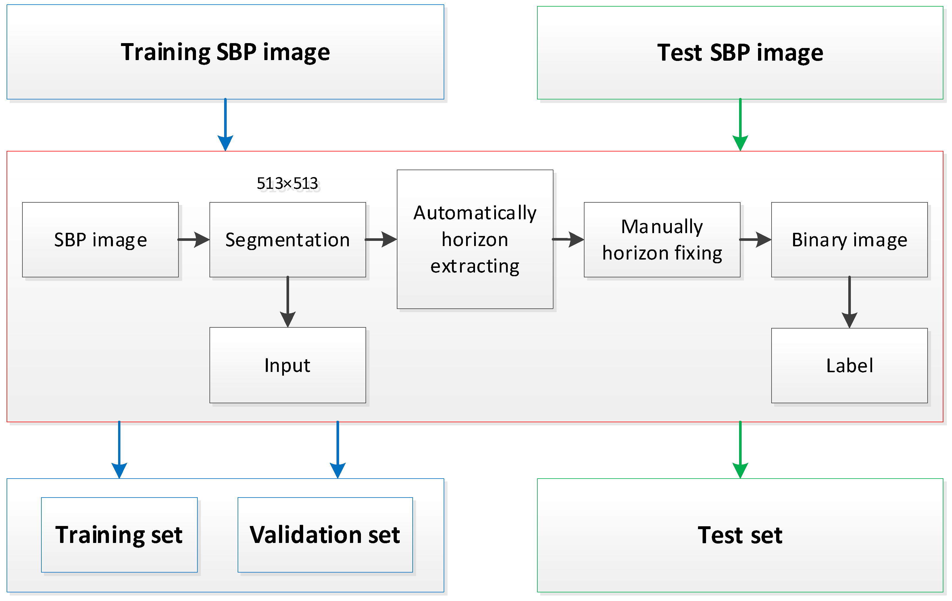
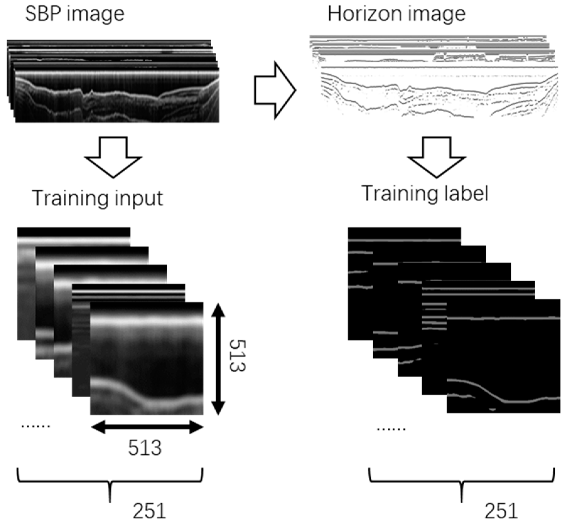
Our task is to extract horizons from an SBP image (Figure 2b). SBP images usually have large sizes and are not suitable for training directly. We split each SBP image into a grid of square tiles (513 × 513 pixels). Each tile is an input to the network for training. The label is the corresponding binary tile in which the pixel values of horizons are one and the others are 0.
Since the number of the horizon class in an SBP image is much less than that of the non-horizon class, binary semantic segmentation becomes a difficult task. Thus, when generating labels, we localize the horizons with a margin of a few pixels of their original location. This processing is not just for improving the imbalanced dataset. It also conforms to the real situation that the sediment from one layer to another changes gradually. Because the length of the utilized boom pulse in this paper is about 400 us and the sampling interval of each pixel in the SBP images is about 50 us, the distinguishable width of the horizons in the SBP images is about 8 pixels. We expand the position of the horizons one pixel up and down and, thus, set the width of the horizons in the labels as 10 pixels, ensuring that the position of horizons in the SBP images are completely covered. Since the identification is achieved as long as some of the pixels (maybe < 8 pixels) of a horizon are recognized, this kind of expansion is appropriate.
The generation process is shown in Figure 3. To make accurate labels, we adopt human-computer interactions to extract horizons (labels). The SNR of the SBP data is usually not high, resulting in the obvious oscillation of gray values in Figure 2c. Although automatic picking can save time and can detect some details, the oscillations bring challenges. Thus, we introduce artificial assistance (human vision) to help improve the accuracy of the training dataset.
Human-computer interaction is particularly effective in reducing the discontinuities of horizons caused by influences of noise and measurement, as shown in Figure 4. After automatic picking, there still exists obvious outliers (the blue ellipse in Figure 4b) and discontinuities (the red ellipse in Figure 4b). Human vision is sensitive to these problems. After manual revision, horizons in Figure 4c are more accurate.
Human-computer interaction, however, is not omnipotent. It can not suppress multiple influences well. Therefore, the labels in the training dataset compose of both real horizons and multiples. The prediction results of the DL identification method also contain both.
2.2.2. Network Architecture and Training
SBP images can be segmented in two parts by the gray level. One is the horizons part, which shows light and represents the strong reflection. Another is the sediment interior part, which shows shade. Thus, horizons picking can be transformed into an image segmentation problem, and the light areas are the position of horizons.
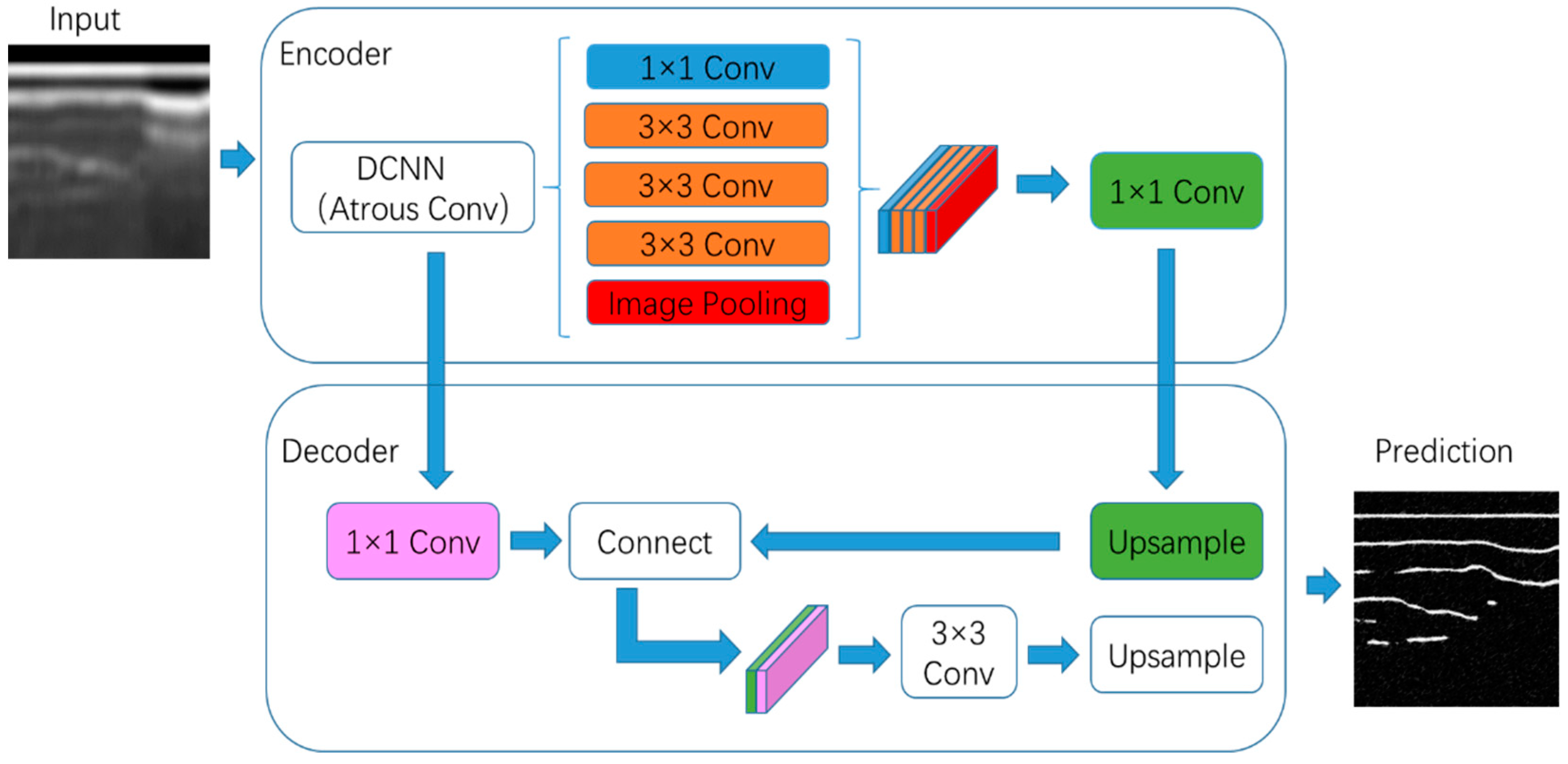
DeeplabV3+ net, a kind of CNN, is prevalently used to accomplish image segmentation. The DeeplabV3+ net is composed of two modules, as shown in Figure 5. One is “Encoder”, which can capture rich semantic information and improve the continuity of the extracted horizons by integrating the surrounding reflection information. Another is “Decoder”, in which horizons show as sharp boundaries in SBP images. The “Decoder” enables the high-level representations to be used to interpret pixel-level content and ensures the accurate trace for horizons. In addition, the DeeplabV3+ net chooses the “atrous convolution”. It can extract features in any resolution. The limitation is only determined by the resource of the computer. These unique characteristics make DeeplabV3+ net suitable for horizon picking. Therefore, we choose the DeeplabV3+ net to train. A more detailed description of DeepLabv3+ can be found in [30].
We give the training dataset to the DeeplabV3+ net and conduct supervised learning to train the network. The learning rate starts from and decays by 10% after every 2000 training steps. During the training process, a validation dataset is used to calculate validation loss.
2.2.3. Evaluation
We adopt the cross-entropy loss function to calculate the difference between the prediction and ground truth. We use MIoU (mean intersection over union) to evaluate the picking accuracy. For each tile, the loss function is defined as:
where is the prediction and is the label.
The accuracy function is:
where and are label values of different categories, represents the number of pixels that belong to the category but are predicted as category. represents the number of pixels correctly identified. Because we have improved the dataset imbalance, the MIoU accuracy is now compatible.
When the training and validation loss values are both small and tend to be stable, and the picking accuracy on the validation dataset no longer increases, then the well-trained model is saved to trace horizons in the observed SBP images.
Our goal is achieved if some pixels of a horizon, in one ping, are recognized. In this case, the MIoU cannot fully represent the accuracy of horizon identification. Here, we introduce another metric, the structural similarity (SSIM), that can measure the structural similarity of the two images. SSIM values the horizons’ form more than its position in a tile. We use the two indicators, MIoU (Formula (2)) and SSIM (Formula (3)), to evaluate the prediction of the observed SBP images (test dataset). MIoU evaluates the quality of network training from the perspective of mathematics, and SSIM evaluates the identification accuracy of horizons from the perspective of geophysics. SSIM includes the evaluation of luminance, contrast, and structure [17]. Since the object to be evaluated in our method is a binary image, the SSIM only contains the evaluation of the structure and can be simplified as:
where x, y represent the identified results by visual interpretation and by the neural network, respectively. is the covariance and is the standard deviation. is a constant and equals 29.2612, calculated by:
where k is a parameter of structural evaluation and equals 0.03. L is the grayscale and equals 255 in our method.
2.3. Multiples Suppression
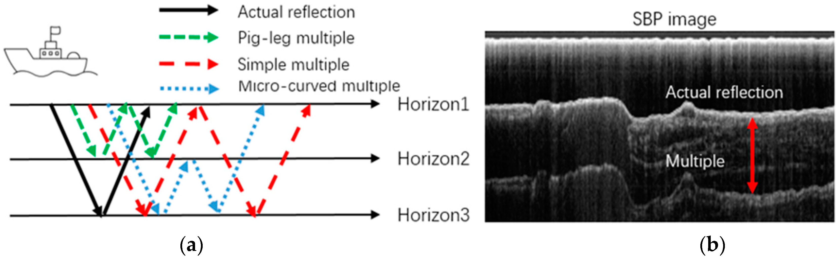
As mentioned in Section 2.2.1, the prediction results of the neural network contain real horizons and multiples. The formation of multiples is caused by sound signals reflecting multiple times at different reflectors and superimposing in the normal sound signal reflection. The common multiples, and the formation process, are shown in Figure 6a. Based on the reflection interface, the multiples can be divided into two kinds, the inter-bed multiples, and the surface-related multiples.
In SBP surveys, there are two especially strong reflection interfaces, sea surface, and sea bottom. The sea surface is the interface between air and liquid. The sea bottom is the interface between liquid and solid. The sound speeds in air, liquid, and solid have a great difference that leads to the strong reflection in their interface. Multiples which have a strong relationship with the sea surface and sea bottom are easy to see in SBP images. In addition, unlike seismic surveys, the sound signal energy is weak, and the propagation distance is short in SBP surveys. Thus, the surface-related multiples (Figure 6b) appear frequently and are obvious, while the inter-bed multiples are always submerged in noise. Surface-related multiples in SBP images have a strong relationship with the instantaneous measurement depth that is the distance from the sea surface to sea bottom [18].
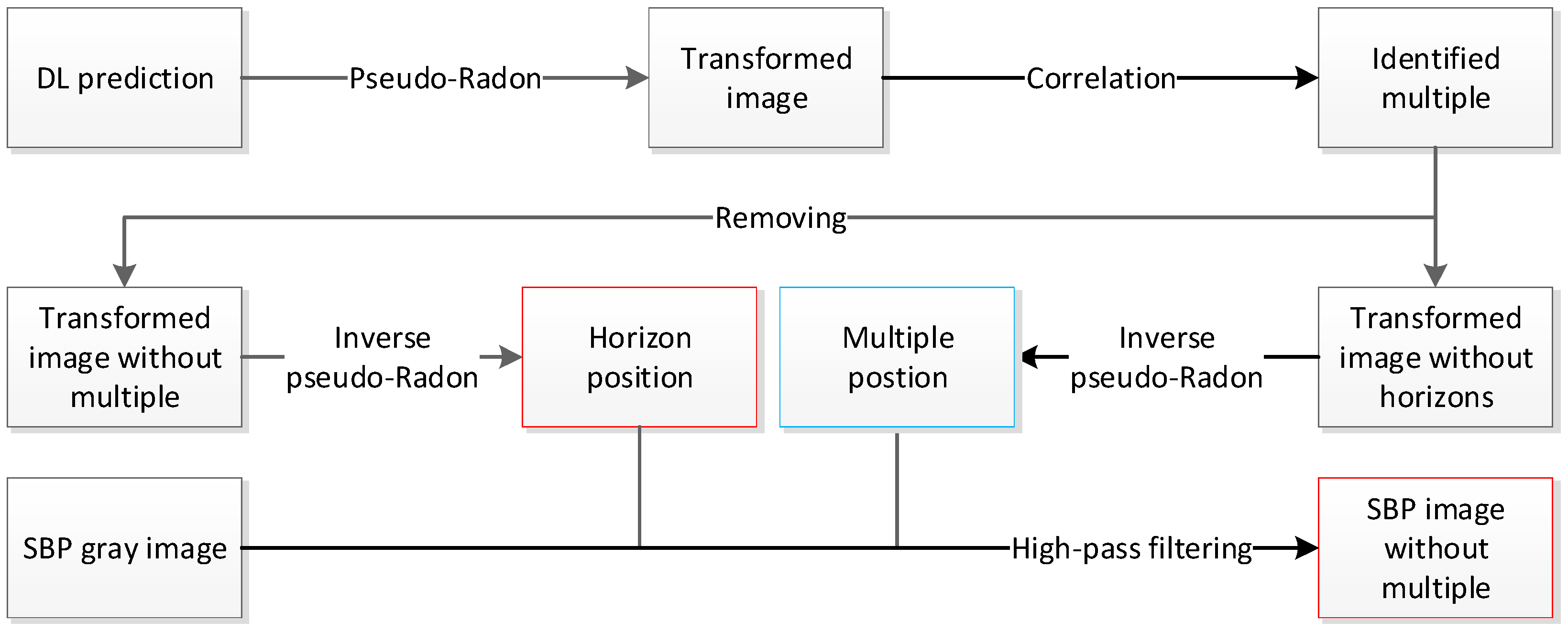
According to the multiples characteristics, we propose a multiple suppression method to eliminate multiples from the DL prediction results. The process of multiple suppression is shown in Figure 7. Referring to the principle of identifying the multiples using Radon transform in multi-channel seismic investigation [31], we propose a kind of transformation (called pseudo-Radon transform) combined with the correlation analysis for identifying the multiples in SBP images.
2.3.1. Pseudo-Radon Transform
In the multi-channel seismic investigation, Radon transform is used to identify the multiples [31]. Because the SBP surveys only have one channel, Radon transform cannot be directly used for the multiple suppression in SBP images. Thus, we propose the pseudo-Radon transform for SBP surveys referring to the principle of Radon transform. Radon transform uses the relationship between the offsets and the multiples to transform the stacked seismic profiles. In pseudo-Radon transform, we transformed the SBP images referencing the relationship between the surface-related multiples and the instantaneous measurement depth.
The pseudo-Radon transform has two steps:
- 8.
- Locate the sea surface and bottom. Because the sea surface and sea bottom are strong reflection interfaces and present two obvious continuous lines in the prediction result of the DL method, it is easy to obtain their accurate position.
- 9.
- Transform the prediction result by the pseudo-Radon transform. We design the pseudo-Radon transform rule as in Equation (5).
After the pseudo-Radon transform, the sea bottom is changed into a straight line. The primary reflections and their corresponding surface-related multiples theoretically are changed into a group of parallel lines (Figure 8). The distance between any two adjacent lines is close to .
2.3.2. Correlation Analysis
Because the multiples have a strong correlation with the corresponding primary reflection in morphological, we propose to calculate the correlation coefficient of the horizons and lines at possible locations to identify the multiples.
As shown in Figure 8d, the positions where the multiples probably appear are
where represents the possible location of multiples, represents the horizon location, and represents an integer.
We calculate the correlation coefficient () of the horizon and the lines at by:
where is the location of the horizon. where is the position in each column. is the location of the line at . is the covariance function. and are variances of and respectively. If is close to 1, we mark the line at as the multiples.
In the prediction results of the DL method, sometimes the lines are not continuous, and noise exists, like Figure 9a. When generating the location sequence ( and ), we first design a box and calculate the line location () in each column in the box:
Since the sea surface and sea bottom can be picked easily in the prediction result, its corresponding surface-related multiples can be found using the proposed suppression method. Then the first unknown line under the sea bottom is marked as the horizon, and we repeat the suppression method until all the lines in the prediction result are marked.
2.3.3. Horizon Refinement
Although we distinguish the multiples and the primary reflection in prediction results, we worry about whether there is sediment information at the multiples positions. Thus, to avoid detail loss, we do not remove the multiples directly.
First, we conduct inverse pseudo-Radon (Equation (8)) for the transformed images and obtain the positions of multiples and primary reflection in the prediction result (a binary image). Then we conduct the high-pass filtering at the position of multiples for a raw SBP image (a gray image). Finally, the filtered image is superimposed with a binary image containing horizons together to generate a new SBP image where the horizon position is clear, and the sediment information is retained.
3. Results
3.1. Data Collection
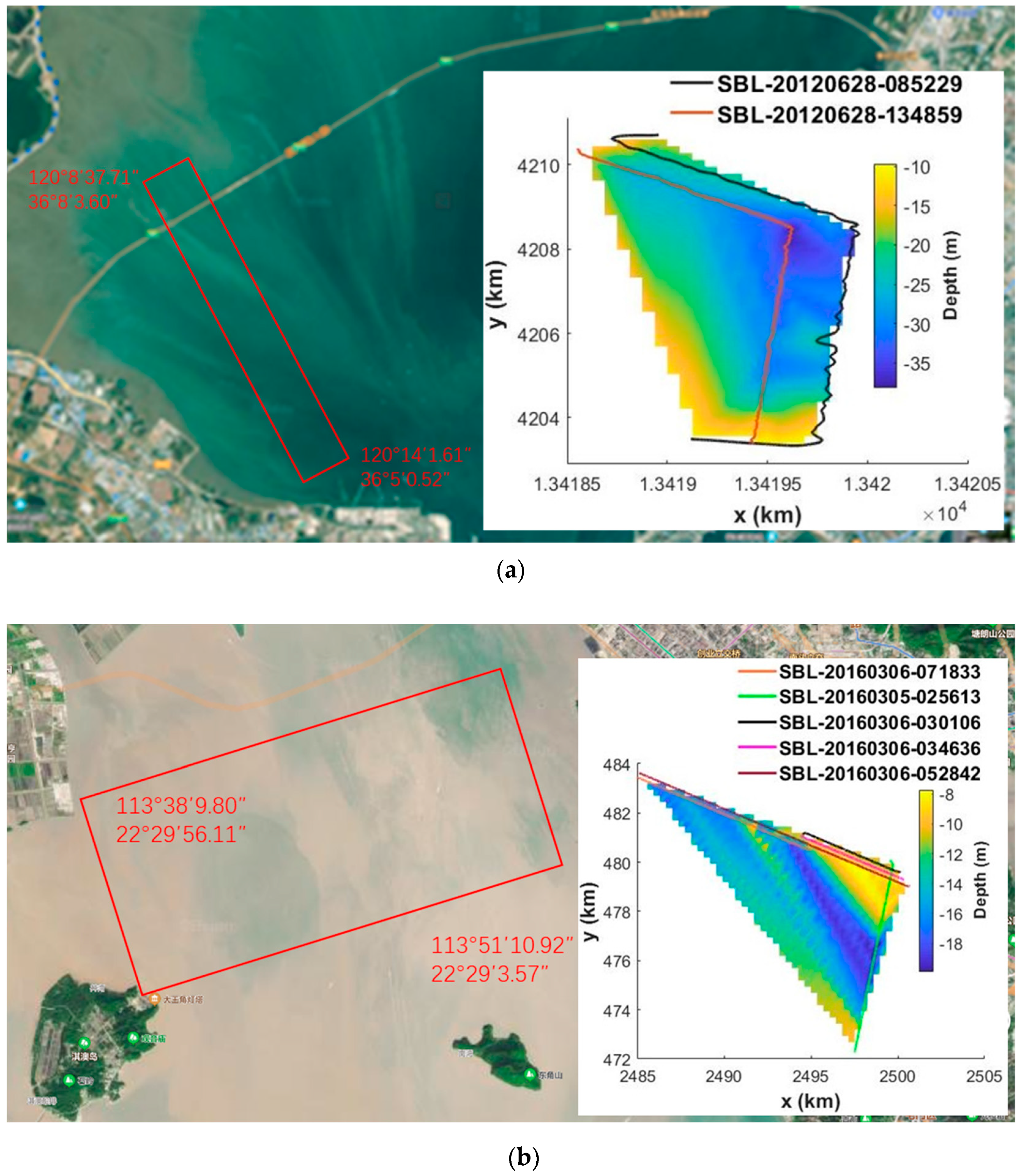
To evaluate the proposed methodology, we chose two groups of SBP images. One was measured in Jiaozhou Bay, Shandong, China, in 2012 (Figure 10a). Another was in Zhujiang Estuary, Guangzhou, China, in 2016 (Figure 10b).
The survey area in Jiaozhou is about 9 km × 1.4 km. The water depth ranges from 10 m to 35 m. There were two survey lines in the area. The length of each line was around 7 km. The distance interval of survey lines was around 150 m. The survey equipment was the C-Boom with a center frequency of 1.76 kHz, detection depth of 70 m (including water depth), and sample interval of 50 μs. The ship speed was about 4–5 knots, which means the distance interval of pings was around 0.5 m.
The survey area in Zhujiang Estuary is about 18 km × 12 km. There were five survey lines. The depth ranges from 8 m to 24 m. The survey equipment was the C-Boom with a center frequency of 1.62 kHz, detection depth of 80 m (including water depth), and sample interval of 50 μs. The ship speed was 4–5 knots.
The size of all SBP images is listed in Table 1.
3.2. DL-Based Identification for Horizons and Multiples
We chose two survey lines, SBL_20120628_085229 (from Jiaozhou Bay) and SBL_20160305_025613 (from Zhujiang Estuary), to form the test dataset. We used other survey lines to generate the training dataset.
3.2.1. Training Dataset
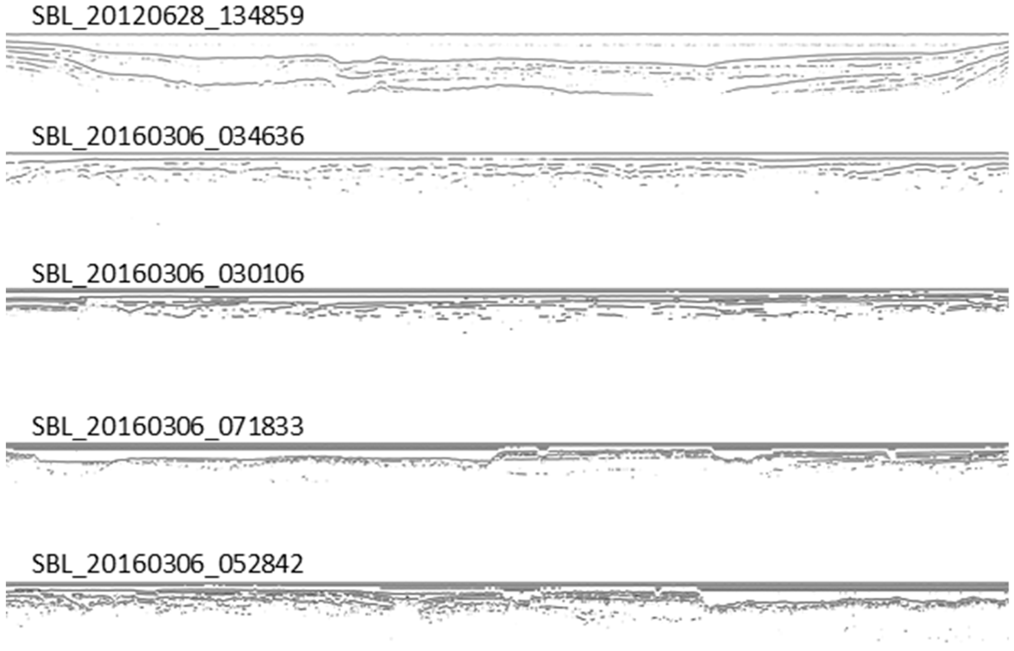
The SBP images for generating training datasets are shown in Figure 11. We picked horizons in these images using the automatic method (Figure 12), and the result is shown in Figure 13.
We split the SBP images (Figure 11) into tiles (513 × 513) as the training inputs. For training labels, we first split the images (Figure 13) that are processed by the automatic picking method into tiles (513 × 513). Then we connected discontinuous horizons and removed obvious outliers in these tiles manually. The recovered tiles are regarded as training labels that have both the objectivity of machine recognition and the accuracy of manual recognition. We obtained 210 training tiles and 90 validation tiles. The process is shown in Figure 14. According to the same process, we used SBL_20120628_085229 and SBL_20160305_025613 to generate a test dataset and obtained 112 test tiles.
3.2.2. The Neural Network Training and the Prediction by the DL Method
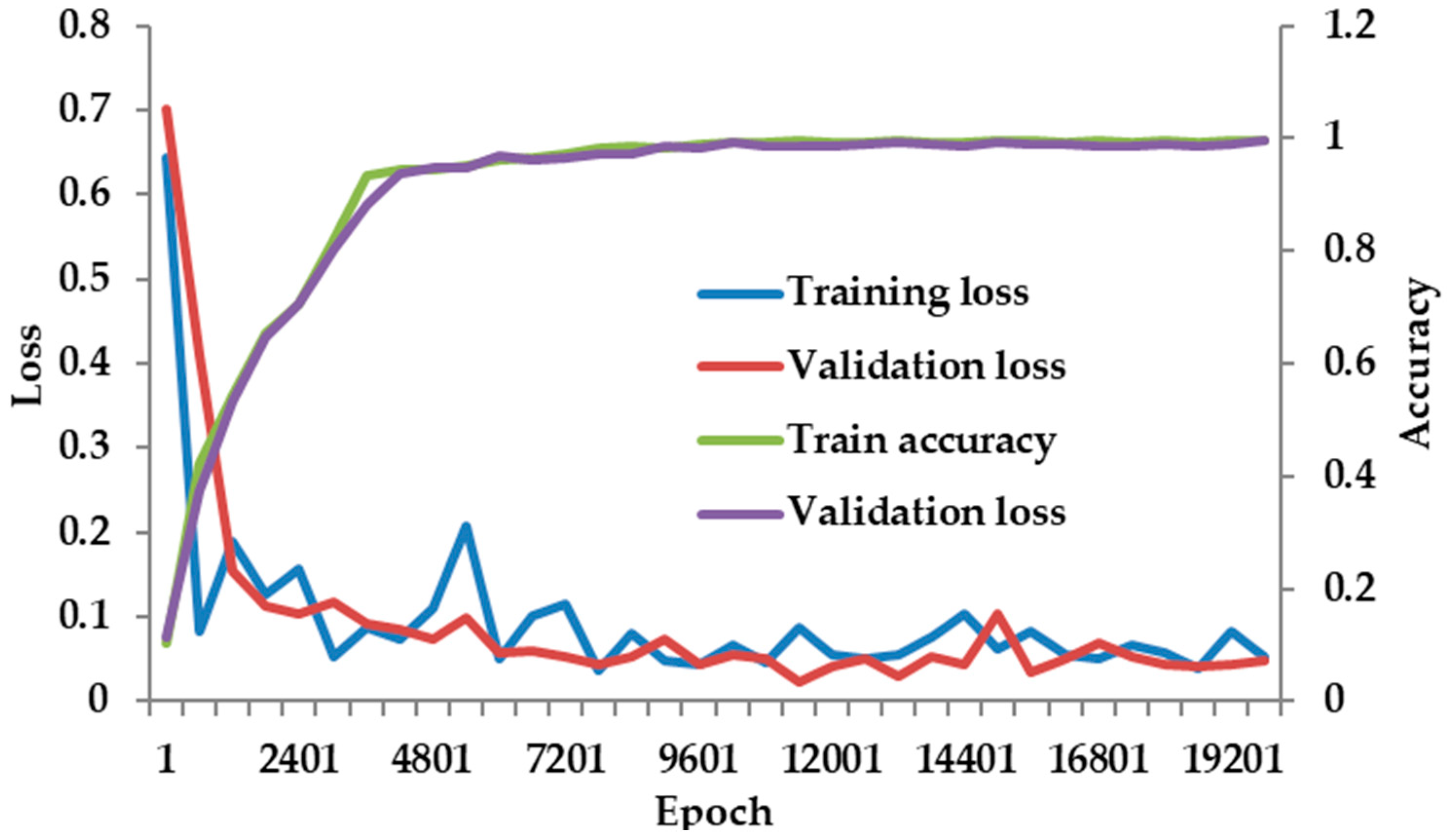
We gave the training dataset and the validation dataset to DeeplabV3+ net to train it. We used a Stochastic Gradient Descent optimizer and set the epochs as 20,000 and the batch size as two. Since the training dataset is small, we initiated the weights of the DeeplabV3+ net using the weights pre-trained on the Pascal VOC dataset to avoid the model from over-fitting. No layer is frozen during the training. The changes of training loss (Equation (1)), validation loss (Equation (1)), and picking accuracy (Equation (2)) are shown in Figure 15. The training loss and validation loss both decreased sharply at first and then gradually increase with the training epochs. The accuracy increases sharply at first and then gradually with the increase of training epochs. The losses become stable after about the 15,000th epoch while the accuracy is still increasing. By comprehensively considering the training efficiency and the changes of loss and accuracy, we chose the trained network at the 19,801st epoch as the well-trained network. At this epoch, both loss and accuracy tend to be stable. The training loss and validation loss equal 0.052605 and 0.047922, respectively. The accuracy is up to 0.996. The small values of the two losses and the high accuracy indicate that the network at the 19,801st epoch is well trained. Especially, the small value of validation loss indicates the well-trained network is not overfitting.
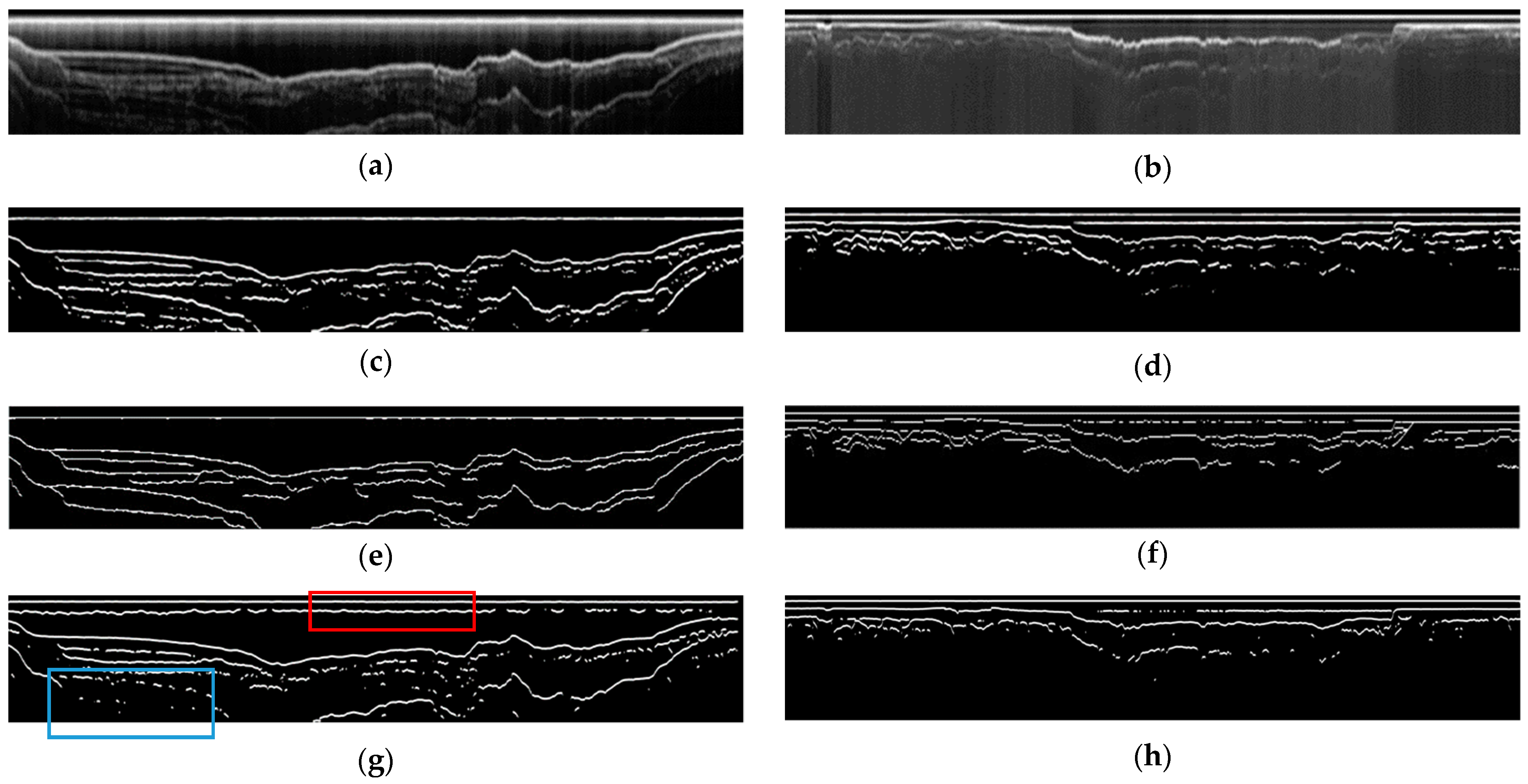
We gave the test dataset to the trained network to pick the horizons and multiples, as shown in Figure 16. Comparing the predictions with the raw images (Figure 16a,b), the horizons and multiples are extracted exactly and completely by the DL method. Furthermore, we used the visual interpretation and the FrangiV algorithm to extract horizons and multiples from the test dataset. The FrangiV algorithm is a new sub-bottom horizon picking algorithm that has shown good performance among SBP data in various surveying environments [16]. The horizons extracted by the visual interpretation are close to the ground truth, and we saw the visual interpretation results as the comparison standard. To quantitatively evaluate the effect of the DL-based identification, we calculated the MIoU (Equation (2)) and SSIM (Equation (3)) of the predictions and the visual interpretation results (Figure 16e,f), the visual interpretation results, and the results of the FrangiV algorithm (Figure 16g,h), respectively. The accuracy indexes are listed in Table 2. Compared with the FrangiV algorithm, the MIoU and SSIM values of our method are higher, indicating our method achieved a higher accuracy. The MIoU and SSIM values of our method are close to 1, indicating the well-trained neural network can achieve the same identification ability as visual interpretation.
3.3. Multiples Suppression
We first used our proposed method to eliminate the surface-related multiples from the prediction of the DL method (Figure 16). Then we compared and analyzed the result with that by the predictive deconvolution to verify the superiority of the proposed method.
3.3.1. Zhujiang and Jiaozhou Surveys
To retain all the information of the prediction results, we set as 140. represents the scaling of the image transformation. If the scaling is too small, the original SBP image will be compressed into a small transformed image, resulting in information loss. Therefore, needs to be set to an appropriate value. Generally, can be set to a value equal to or greater than the maximum of the seafloor depth in the survey area.
We employed pseudo-Radon transform (Equation (5)) for the prediction results (Figure 16b,d) and obtained the transformed images (Figure 17a,b). In the transformed images, the sea bottom is changed into a straight line, and its corresponding surface-related multiples are paralleled below.
We employed correlation analysis for the transformed images and distinguished the multiples (red lines) and primary reflections (black lines) in Figure 17a,b. We removed multiples from the transformed images, employed inverse pseudo-Radon transform for the images without multiples, and then obtained Figure 17c,d. Figure 17c,d only contain horizons.
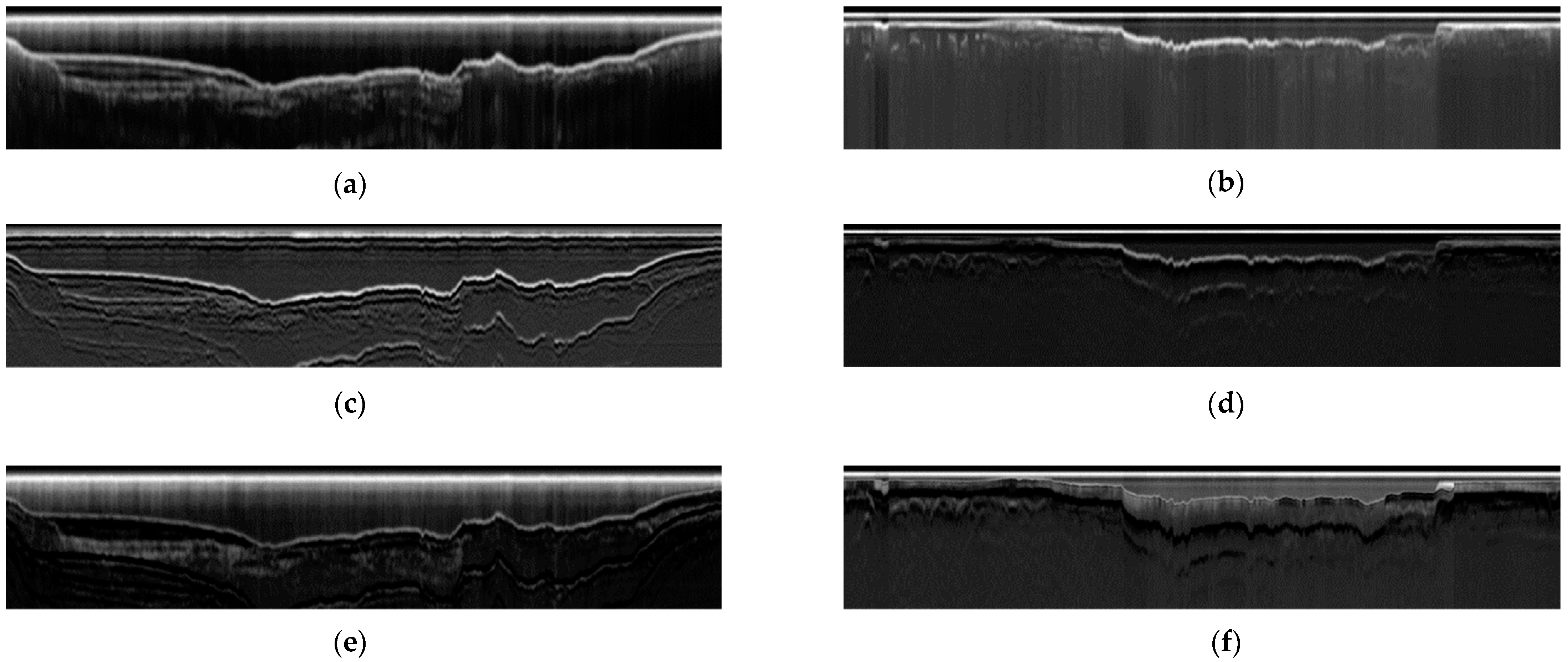
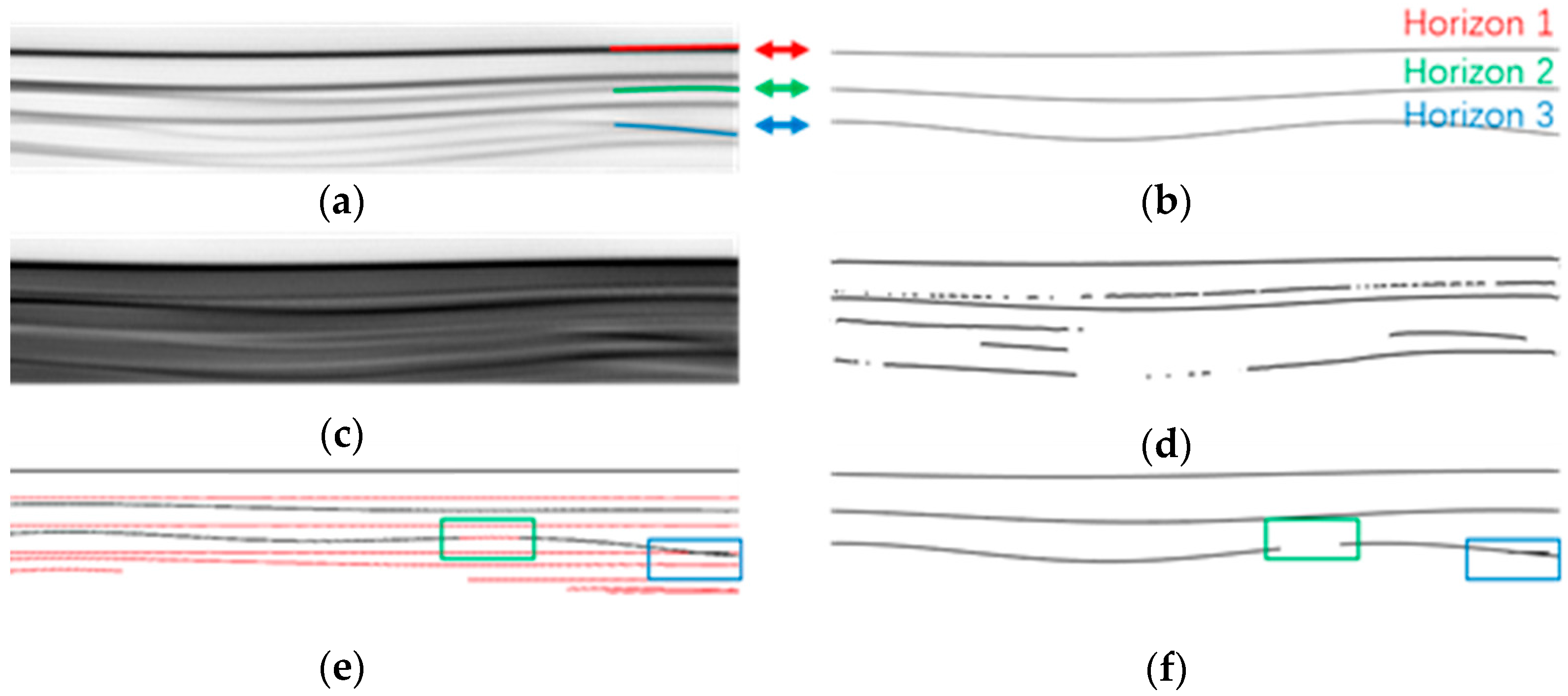
Next, we utilized Figure 16a,c and Figure 17a,b to conduct horizon refinement (Section 2.3.3) and got the final results (Figure 18a,b). Figure 18a,b are the results by eliminating the multiples and highlight the primary reflection. Compared with Figure 17c,d, Figure 18a,b retain the sediment details in the regions of multiples. Thus, we regarded Figure 18a,b as our final picking results to offer comprehensive geological information for the survey area.
3.3.2. Methods Comparison
To verify the superiority of the proposed multiple suppression method, we used predictive deconvolution, a prevalent method for multiple suppression, for SBP images of SBL_20120628_085229 and SBL_20160305_025613 and compared the results (Figure 18c,d).
There are still multiples left in Figure 18c,d. Predictive deconvolution cannot eliminate multiples completely. The order of multiple suppression effects from good to bad is the proposed method, predictive deconvolution (step = instantaneous seawater depth), and deconvolution (step = 25). The predictive step represents the possible location of multiples. The more accurate the step is, the better the result of predictive deconvolution is. Thus, the predictive deconvolution result with the step of instantaneous seawater depth is better than that with the step of a fixed value.
Predictive deconvolution cannot completely calculate the multiples morphological changes produced during the acoustic signal propagating in the geological structure. It results in location mismatch during the prediction subtraction. The multiples, therefore, cannot be eliminated completely by predictive deconvolution.
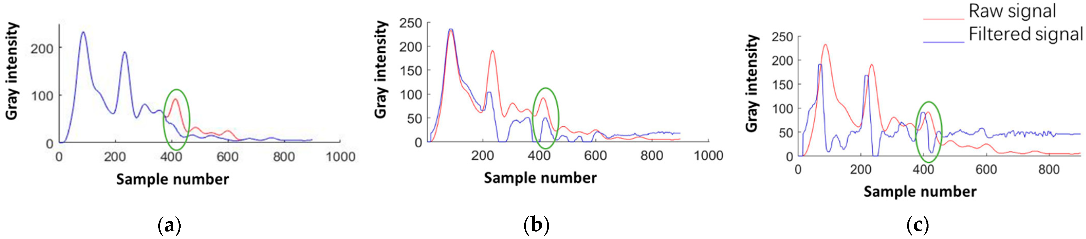
To intuitively show the performances of the two methods, we compared the reflection sequence of one ping before and after the methods in Figure 19. Because we accurately found the multiples and conducted high-pass filtering in the multiples region rather than removed the multiples directly, our proposed method effectively suppressed the multiples and retained some signal details (the blue line in the ellipse in Figure 19a). The location mismatch caused by predictive deconvolution is obvious in Figure 19b,c. Due to the location mismatch, there are still residual multiples in the ellipse in Figure 19b,c and the raw signal is damaged.
Since the predictive deconvolution failed to eliminate the multiples accurately for the two test survey lines, continuing to extract horizons does not make much sense. The existing methods for identifying horizons suppress the multiples first and then extract the horizons. The bad performance of the predictive deconvolution will directly bring errors to the next extraction. To further quantitatively evaluate the performance of the proposed multiples suppression method, we conducted a synthesis experiment in which we compared the extracted horizons by our method and the predictive deconvolution with the ground truth.
We assumed three horizons (Figure 20b) and simulated a corresponding SBP image (Figure 20a) based on the principle of multiples generation and energy attenuation [22,32]. Then we employed the predictive deconvolution and the proposed multiples suppression method for the virtual SBP image. The suppression results are shown in Figure 20. Both methods can identify the horizons, but the multiples are not removed completely by the predictive deconvolution. In addition to the stronger ability to remove multiples, our method also improves the problem of horizon discontinuities (comparing Figure 20d and Figure 20f). To further quantitatively evaluate our method, we calculated MIoU (Equation (2)) and SSIM (Equation (3)) of the ground truth and the predictive deconvolution results (Figure 20d), then the ground truth and results of our method (Figure 20f), respectively. The accuracy indexes are listed in Table 3. Through the comparison of the MIoU and SSIM values, it is verified that our method can achieve higher accuracy. The identified horizons of our method, however, still deviate a little from the ground truth. Part of the horizons are missing (the green rectangle in Figure 20f), and the nonexistent horizons appear (the blue rectangle in Figure 20f).
4. Discussion
4.1. Obtaining Discontinuous Horizons Using Multiples
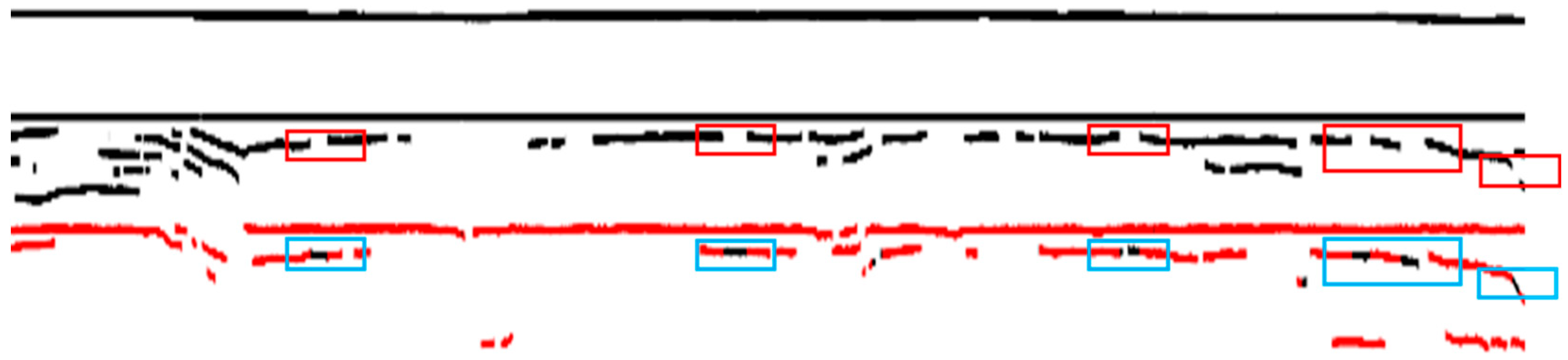
The horizons in SBP images are sometimes lost (Figure 9) due to the noise, broken channels, or other problems during the SBP measurement. Although we revise the discontinuity of horizons manually when generating training datasets, there may be omissions. The lost horizons will lead to incomplete extraction of surface-related multiples since we trace the multiples according to the correlation of it with the horizons.
Figure 21 is a part of SBL_20120628_085229 (Figure 17a) after horizons picking. It can be discovered that there are several discontinuities of multiples (blue rectangles) that should have been continuous, and the multiples are connected to the horizons. This phenomenon is caused by the discontinuity of the corresponding horizons (red rectangles). We can utilize the multiples discontinuity to detect and then recover the horizons discontinuity. The specific steps are as follows.
- 10.
- Recover the multiples discontinuity. Search the position of horizons connected with multiples and mark the horizons as multiples.
- 11.
- Recover the horizon discontinuity. Determine the position of horizon discontinuity according to the position of multiples discontinuity and recover the horizon discontinuity according to the shape of the recovered multiple.
4.2. The Specialty of the Proposed Method
Most DL-based methods for identification tasks directly output the target location [27,33,34]. Unlike these conventional methods, our proposed method combines the data-driven DL method with the model-driven physical methods to pick the horizons. The prediction of our well-trained DeeplabV3+ network is not the horizon that we want to get finally. The prediction contains both multiples and primary reflections. To obtain the final horizons, we eliminate the multiples from the prediction by the proposed multiple suppression method. Although the combination of the data-driven method and model-driven method will reduce the execution efficiency compared with the pure data-driven one, it improves the reliability and accuracy of the identified horizons. Since the characteristics of multiples and horizons are quite similar, especially from a perspective of image processing, it is difficult to only extract the horizons from an SBP image directly by DL methods.
Another specialty of the proposed method is the form of its final results. The target of horizon picking is to determine the location of the horizons in an SBP image. In theory, when we successfully distinguish the multiples and the primary reflections in the prediction of the DeeplabV3+ network (Section 2.3.2), the identification task is completed. We, however, continued on to add a step (Section 2.3.3 Horizon Refinement) to further deal with the signals at multiples positions. We worried that there might be sediment information at the positions of multiples. If the signals at the positions of multiples are removed directly, the information covered by multiples will also be removed, leading to detail loss. Therefore, we proposed to conduct the high-pass filtering at the position of multiples for a raw SBP image and superimpose the filtered image with a binary image only containing horizons to generate a new SBP image. This processing method can avoid the distortion of the original signals, as shown in Figure 19. We regard the new image as the final result of horizon picking. In this new image, the multiples are suppressed, the horizons are clear, and the sediment information at the positions of multiples is retained. However, if only the positions of horizons are needed, the refinement step (Section 2.3.3 Horizon Refinement) can be skipped.
5. Conclusions
We proposed a physicals-combined deep learning method to pick horizons from SBP images using the DeeplabV3+ net. The prediction of the trained model includes primary reflections and multiples. We further used the proposed pseudo-Radon transform and correlation analysis for the prediction and distinguished the horizons and surface-related multiples. The feasibility and accuracy of this method were verified by two field surveys, the Zhujiang and Jiaozhou surveys. The trained DeeplabV3+ model can extract horizons and multiples accurately and quickly from an SBP image. The proposed multiple suppression can efficiently eliminate the surface-related multiples and achieve a better performance compared with the predictive deconvolution. Our proposed method can not only pick horizons accurately but also avoid losing sediment details. Furthermore, the picked multiples can help recover the discontinuity of horizons.
Author Contributions
Conceptualization, J.F.; methodology, J.F. and G.Z.; software, G.Z.; validation, S.L.; formal analysis, J.Z.; investigation, S.L.; resources, J.Z.; data curation, J.Z.; writing—original draft preparation, J.F.; writing—review and editing, J.F. and S.L.; visualization, G.Z.; supervision, J.Z.; project administration, J.F.; funding acquisition, J.Z. All authors have read and agreed to the published version of the manuscript.
Funding
This research was funded by the National Natural Science Foundation of China under Grant 41576107, Grant 42176186, and Grant 41376109, in part by the National Key R&D Program of China under Grant 2016YFB0501703.
Data Availability Statement
The data of Jiaozhou Bay were offered by Tianjin Maritime Surveying and Mapping Center, Beihai navigation support center, Ministry of transport. Address: No. 21, Yujiang Road, Hexi District, Tianjin, China. Telephone: +86-18920832298 (Peng Dou). The data of Zhujiang estuary were offered by the first Institute of Oceanography, State Oceanic Administration. Address: No. 6, Xianxialing Road, Laoshan District, Qingdao, China. Telephone: +86-0532-88967420 8 (Jia Yu). The data can be obtained by applying to the center and institute.
Acknowledgments
We would like to thank our colleagues for their helpful suggestions during the experiment and thank the editor and the anonymous reviewers for their valuable comments and suggestions that greatly improve the quality of this paper. We also thank the Key R&D Program of China Communications Construction Company under Grant 2019-ZJKJ-ZDZX-01-0349.
Conflicts of Interest
The authors declare no conflict of interest.
References
- Cukur, D.; Krastel, S.; Cagatay, M.N.; Damcı, E.; Meydan, A.F.; Kim, S.P. Evidence of extensive carbonate mounds and sublacustrine channels in shallow waters of Lake Van, eastern Turkey, based on high-resolution chirp subbottom profiler and multibeam echosounder data. Geo-Mar. Lett. 2015, 35, 329–340. [Google Scholar] [CrossRef]
- Li, S.J.; Chu, F.Y.; Fang, Y.X.; Wu, Z.Y. Associated interpretation of sub-bottom and single-channel seismic profiles from Shenhu Area in the north slope of South China Sea—characteristic of gas hydrate sediment. Adv. Mat. Res. 2011, 217, 1430–1437. [Google Scholar] [CrossRef]
- Kim, Y.J.; Koo, N.H.; Cheong, S.; Kim, J.K.; Chun, J.H.; Shin, S.R.; Riedel, M.; Lee, H.Y. A case study on pseudo 3-D Chirp sub-bottom profiler (SBP) survey for the detection of a fault trace in shallow sedimentary layers at gas hydrate site in the Ulleung Basin, East Sea. J. Appl. Phys. 2016, 133, 98–115. [Google Scholar] [CrossRef]
- Ding, W.F.; Luo, J.H.; LAI, X.H.; Gou, Z.K.; Fu, X.M. The research of interactive interpretation picking for sub-bottom profile. Mar. Sci. 2008, 32, 1–6. [Google Scholar]
- Tan, C.; Zhang, X.B.; Yang, P.X.; Sun, M. A Novel Sub-Bottom Profiler and Signal Processor. Sensors 2019, 19, 5052. [Google Scholar] [CrossRef] [Green Version]
- Plets, R.M.K.; Dix, J.K.; Adams, J.R.; Bull, J.M.; Henstock, T.J.; Gutowski, M.; Best, A.I. The use of a high-resolution 3D Chirp sub-bottom profiler for the reconstruction of the shallow water archaeological site of the Grace Dieu (1439), River Hamble, UK. J. Archaeol. Sci. 2009, 36, 408–418. [Google Scholar] [CrossRef]
- Nakamura, K.; Machida, S.; Okino, K.; Masaki, Y.; Iijima, K.; Suzuki, K.; Kato, Y. Acoustic characterization of pelagic sediments using sub-bottom profiler data: Implications for the distribution of REY-rich mud in the Minamitorishima EEZ, western Pacific. Geochem. J. 2016, 50, 605–619. [Google Scholar] [CrossRef] [Green Version]
- Cao, X.H.; Qu, Z.G.; Shen, B.J.; Zhang, H.Y. Illuminating centimeter-level resolution stratum via developed high-frequency sub-bottom profiler mounted on Deep-Sea Warrior deep-submergence vehicle. Mar. Georesour. Geotec. 2020. [Google Scholar] [CrossRef]
- Bondar, I. Seismic horizon detection using image processing algorithms. Geophys. Prospect. 1992, 40, 785–800. [Google Scholar] [CrossRef]
- Maroni, C.S.; Quinquis, A.; Vinson, S. Horizon Picking on Subbottom Profiles Using Multiresolution Analysis. Digit. Signal. Process. 2001, 11, 269–287. [Google Scholar] [CrossRef]
- Zhao, J.H.; Li, S.B.; Zhang, H.M.; Feng, J. Comprehensive Sediment Horizon Picking From Subbottom Profile Data. IEEE J. Ocean. Eng. 2018, 44, 524–534. [Google Scholar] [CrossRef]
- Fakiris, E.; Blondel, P.; Papatheodorou, G.; Christodoulou, D.; Dimas, X.; Georgiou, N.; Kordella, S.; Dimitriadis, C.; Rzhanov, Y.; Geraga, M.; et al. Multi-Frequency, Multi-Sonar Mapping of Shallow Habitats—Efficacy and Management Implications in the National Marine Park of Zakynthos, Greece. Remote Sens. 2019, 11, 461. [Google Scholar] [CrossRef] [Green Version]
- Dossi, M.; Forte, E.; Pipan, M. Automated reflection picking and polarity assessment through attribute analysis: Theory and application to synthetic and real ground-penetrating radar data. Geophysics 2015, 80, 23–35. [Google Scholar] [CrossRef]
- Forte, E.; Dossi, M.; Pipan, M.; Del Ben, A. Automated phase attribute-based picking applied to reflection seismics. Geophysics 2016, 81, 141–150. [Google Scholar] [CrossRef]
- Zhao, J.H.; Li, S.B.; Zhao, X.; Feng, J. A Comprehensive Horizon-Picking Method on Subbottom Profiles by Combining Envelope, Phase Attributes, and Texture Analysis. Earth Space Sci. 2020, 7, e2019EA000680. [Google Scholar] [CrossRef] [Green Version]
- Li, S.B.; Zhao, J.H.; Zhang, H.M.; Bi, Z.J.; Qu, S.H. A Novel Horizon Picking Method on Sub-Bottom Profiler Sonar Images. Remote Sens. 2020, 12, 3322. [Google Scholar] [CrossRef]
- Wang, Z.; Bovik, A.C.; Sheikh, H.R.; Simoncelli, E.P. Image quality assessment: From error visibility to structural similarity. IEEE Trans. Image Process. 2004, 13, 600–612. [Google Scholar] [CrossRef] [PubMed] [Green Version]
- Berkhout, A.J.; Verschuur, D.J. Imaging of multiple reflections. Geophysics 2006, 71, SI209–SI220. [Google Scholar] [CrossRef]
- Muijs, R.; Robertsson, J.O.A.; Holliger, K. Prestack depth migration of primary and surface-related multiple reflections: Part I—Imaging. Geophysics 2007, 72, 59–69. [Google Scholar] [CrossRef]
- Slob, E.; Zhang, L.L. Unified elimination of 1D acoustic multiple reflection. Geophys. Prospect. 2021, 69, 327–348. [Google Scholar] [CrossRef]
- Wang, X.; Xia, C.L.; Liu, X.W. A case study: Imaging OBS multiples of South China Sea. Mar. Geophys. Res. 2012, 33, 89–95. [Google Scholar] [CrossRef]
- Verschuur, D.J. Seismic Multiple Removal Techniques—Past, Present and Future; EAGE Publications: Houten, The Netherlands, 2006; pp. 37–119. [Google Scholar]
- Imamverdiyev, Y.; Sukhostat, L. Lithological facies classification using deep convolutional neural network. J. Pet. Sci. Eng. 2019, 174, 216–228. [Google Scholar] [CrossRef]
- Feng, Q.; Miao, Y.; Xiao, Y.L.; Yao, J.W.; Cai, L.; Guang, M.H. Unsupervised seismic facies analysis via deep convolutional autoencoders. Geophysics 2018, 83, A39–A43. [Google Scholar]
- Maxwell, A.E.; Warner, T.A.; Guillén, L.A. Accuracy Assessment in Convolutional Neural Network-Based Deep Learning Remote Sensing Studies—Part 1: Literature Review. Remote Sens. 2021, 13, 2450. [Google Scholar] [CrossRef]
- Park, C.I.; Sohn, C.B. Data Augmentation for Human Keypoint Estimation Deep Learning based Sign Language Translation. Electronics 2020, 9, 1257. [Google Scholar] [CrossRef]
- Feldens, P.; Darr, A.; Feldens, A.; Tauber, F. Detection of Boulders in Side Scan Sonar Mosaics by a Neural Network. Geosciences 2019, 9, 159. [Google Scholar] [CrossRef] [Green Version]
- Nguyen, H.T.; Lee, E.H.; Lee, S. Study on the Classification Performance of Underwater Sonar Image Classification Based on Convolutional Neural Networks for Detecting a Submerged Human Body. Sensors 2020, 20, 13. [Google Scholar] [CrossRef] [Green Version]
- Cheng, B.; Li, Z.; Xu, B.; Yao, X.; Ding, Z.; Qin, T. Structured Object-Level Relational Reasoning CNN-Based Target Detection Algorithm in a Remote Sensing Image. Remote Sens. 2021, 13, 281. [Google Scholar] [CrossRef]
- Chen, L.C.; Zhu, Y.; Papandreou, G.; Schroff, F.; Adam, H. Encoder-Decoder with Atrous Separable Convolution for Semantic Image Segmentation, In Proceedings of the European conference on computer vision (ECCV), Munich, Germany, 8–16 October 2018, 833–851.
- Shankar, U.; Singh, S.S.; Sain, K. Signal enhancement and multiple suppression using Radon transform: An application to marine multichannel seismic data. Mar. Geophys. Res. 2009, 30, 85–93. [Google Scholar] [CrossRef]
- Lurton, X. An Introduction to Underwater Acoustics: Principles and Applications, 2nd ed.; Springer: New York, NY, USA, 2010. [Google Scholar]
- Zheng, G.; Zhang, H.; Li, Y.; Zhao, J. A Universal Automatic Bottom Tracking Method of Side Scan Sonar Data Based on Se-mantic Segmentation. Remote Sens. 2021, 13, 1945. [Google Scholar] [CrossRef]
- Zhao, P.; Liu, K.; Zou, H.; Zhen, X. Multi-Stream Convolutional Neural Network for SAR Automatic Target Recognition. Remote Sens. 2018, 10, 1473. [Google Scholar] [CrossRef] [Green Version]
Figure 1.
The workflow of horizon picking from SBP images. (1) We transfer the collected SEG-Y data to SBP images by data decoding and image processing. (2) We generate a training dataset using SBP images and utilize the dataset to train a neural network. (3) We employ the trained network to predict horizons from observed SBP images, which we exclude from the training dataset. (4) We eliminate the multiples from the prediction using the proposed multiple filtering method and obtain the final horizons.

Figure 2.
SBP survey. (a) The sonar of an SBP system converts the control signals to acoustic pulses (100 Hz–20 kHz) and emits the pulses towards the seafloor. After the pulse hits the sediment, acoustic energy reflected from the horizons is received by the transducer and is recorded as a time series called “ping”. (b) The ping is converted to a series of gray values, and all the adjacent pings compose an SBP image. (c) One ping reflection sequence. The three peak values of gray level correspond to the horizons in (b).

Figure 3.
Generation process for training dataset. SBP images are broken into tiles. Each tile is an input to the neural network. For each tile, the horizon locations are tracked by the automatic method first and then are examined and restored artificially. Afterward, we create a tile of the same dimension as the input and fill the horizon locations with gray values of 1 and the remaining locations with 0. The corresponding binary tile is the label. All the data are divided into 2 groups, training dataset and validation dataset, according to the ratio of 3:1.

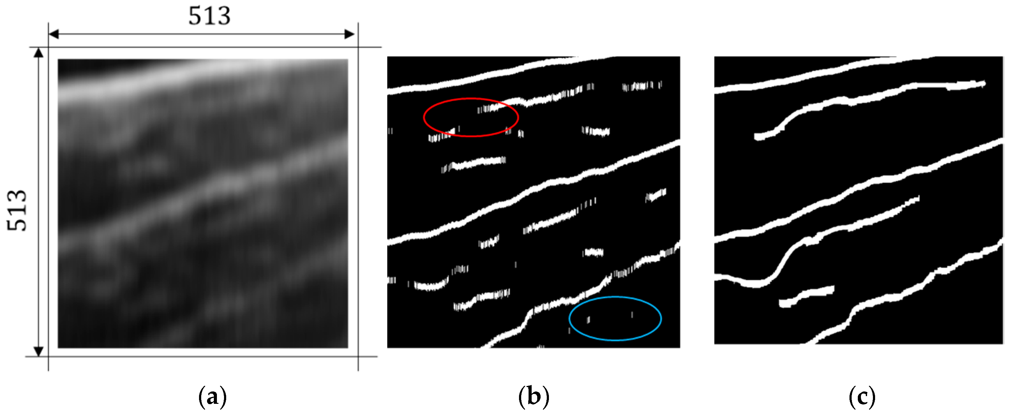
Figure 4.
Human-computer interaction. (a) An input. (b) The corresponding tile to the input tile after automatic horizons extraction. The white pixels are extracted horizons. (c) A label. The tile after artificial recovery. The label is the corresponding binary tile in which the pixel values of horizons are 1, and the others are 0. The width of the horizon is 10 pixels. The noise in (b) is removed manually, such as the white part in the blue ellipse. The obvious discontinuities of horizons are connected manually, such as the discontinuity in the red ellipse.

Figure 5.
The architecture of the DeeplabV3+ net. DeepLabv3+ contains an encoder-decoder structure. “DCNN” represents deep convolutional neural networks. “Conv” represents the convolutional layer. The number before “Conv”, such as “3 × 3”, represents the size of the convolution kernel.
Figure 5.
The architecture of the DeeplabV3+ net. DeepLabv3+ contains an encoder-decoder structure. “DCNN” represents deep convolutional neural networks. “Conv” represents the convolutional layer. The number before “Conv”, such as “3 × 3”, represents the size of the convolution kernel.

Figure 6.
The type of multiples.

Figure 7.
The process of multiple suppression. (1) Convert the DL prediction (a binary image containing horizons and multiples) to the transformed image using pseudo-Radon transform. (2) Distinguish the multiples and horizons in the transformed image according to correlation analysis. (3) Employ inverse pseudo-Radon transform for the transformed image and obtain the position of horizons and multiples. (4) Conduct the high-pass filtering for the position of multiples in the SBP image (a gray image). (5) Superimpose the filtered image and the binary image containing horizons.

Figure 8.
Pseudo-Radon transform. (a) The formation mechanism of horizons and multiples. The propagation path of the signal in the black dotted rectangle depicts the formation of the horizon. The propagation path in the red dotted rectangle depicts the formation of the multiples. In the red dotted rectangle, the red path is the equivalent form of the black path. According to the formation mechanism of the multiples, h1 = h2. (b) The reflection sequence of one ping. The rectangle is the sea bottom, and the ellipse is the double surface-related multiples. The signal shapes in the rectangle and the ellipse are similar. (c) A prediction result of the DL method. It is a binary image containing the multiples and horizons. (d) A transformed image. The horizon, double multiples, and triple multiples are approximately parallel. The spacing between adjacent lines is close to s, the scaling parameter in pseudo-Radon transform.

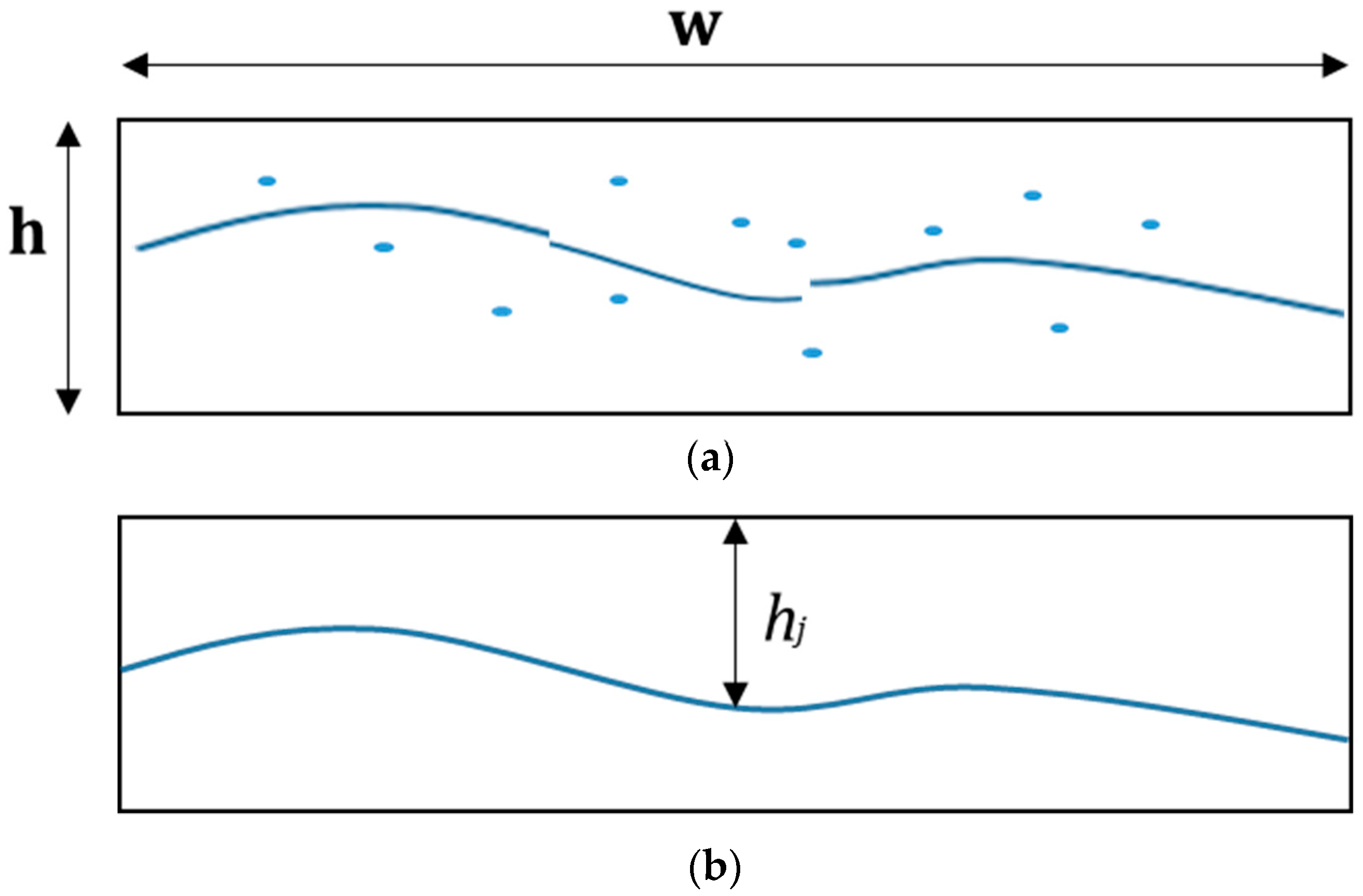
Figure 9.
The gray gravity center method. (a) A box of the location sequence. The blue dots are the noise. In the box the extracted horizon is not continuous. (b) A box after calculating. represents the horizon location in each column in the box. After determining the horizon location, noise is eliminated and the horizon is continuous.

Figure 10.
Survey areas. (a) Jiaozhou Bay. (b) Zhujiang Estuary. The coordinate system of longitudes and latitudes is WGS-84. The red rectangles represent the survey areas. The illustrations are the corresponding topographic map. The coordinate system of x and y is a local system.
Figure 10.
Survey areas. (a) Jiaozhou Bay. (b) Zhujiang Estuary. The coordinate system of longitudes and latitudes is WGS-84. The red rectangles represent the survey areas. The illustrations are the corresponding topographic map. The coordinate system of x and y is a local system.

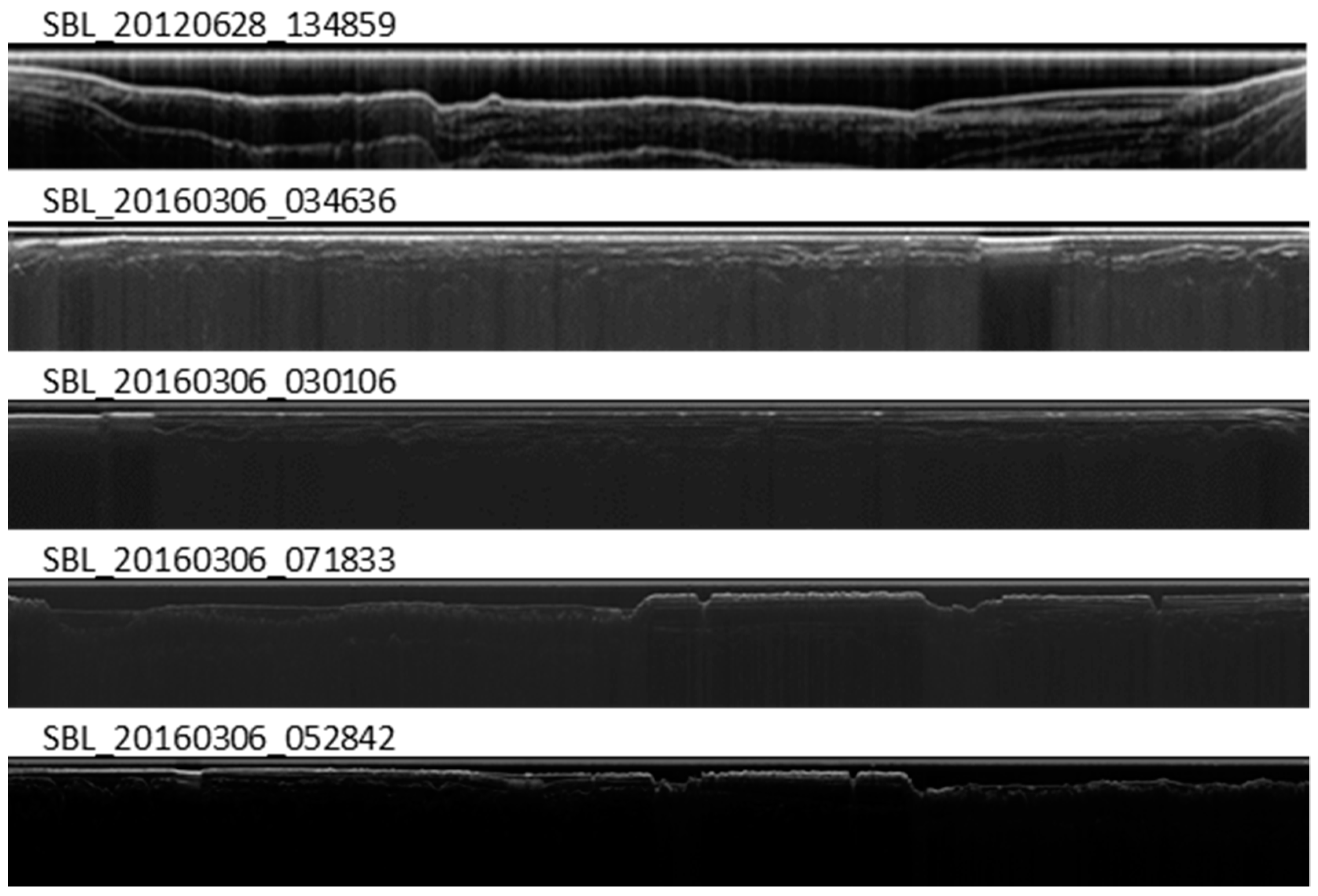
Figure 11.
SBP images for training dataset.

Figure 12.
The process of automatic horizon picking.

Figure 13.
The horizons extracted by the automatic method.

Figure 14.
The generation process of the training dataset.

Figure 15.
Training process.

Figure 16.
The identified horizons and multiples. In (a,b), the test inputs, are the raw SBP images numbered SBL_20120628_085229 and SBL_20160305_025613, respectively. In (c,d) are the predictions of (a,b), respectively. The predictions are binary images and contain the identified multiples and horizons. In (e,f) are the identified multiples and horizons by visual interpretation for (a,b), respectively. In (g,h) are the identified multiples and horizons by the FrangiV algorithm for (a,b), respectively. The horizons in the red rectangle are false, and the horizons discontinuity in the blue rectangle is true.

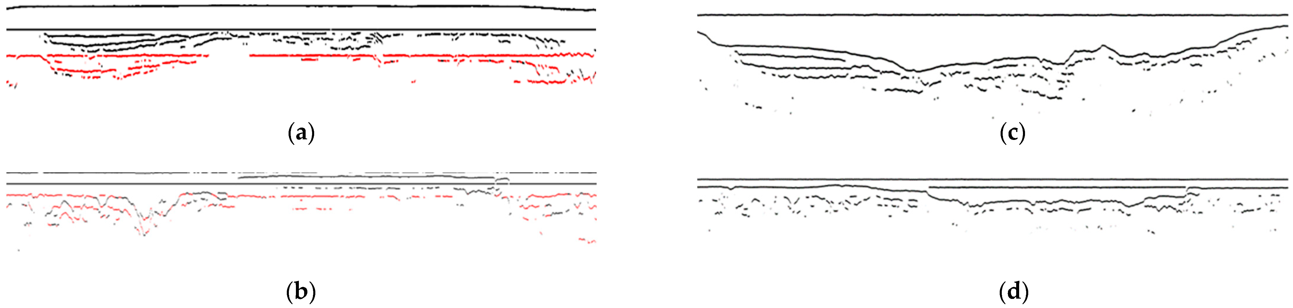
Figure 17.
Distinguishing between horizons and multiples. (a) (SBL_20120628_085229) and (b) (SBL_20160305_025613) are the transformed images by pseudo-Radon transform. The red lines are the identified multiples; the black lines are horizons. (c) (SBL_20120628_085229) and (d) (SBL_20160305_025613) are the inverse pseudo-Radon transformed images after multiples removal.

Figure 18.
Comparison of multiple suppression results. (a,c,e) represent SBL_20120628_085229. (b,d,f) represent SBL_20160305_025613. (a,b) are the results of the proposed multiple suppression method. (c~f) are the results of predictive deconvolution. The predictive step of (c,f) is 25, and the step of (e,f) equals instantaneous seawater depth.

Figure 19.
The reflection sequence of one ping. (a) Result by our proposed method. (b) Result by predictive deconvolution in which the predictive step is instantaneous seawater depth. (c) Result by predictive deconvolution in which the predictive step equals 25. The red lines represent the raw signal. The blue lines represent the signal after multiples suppression method. The green ellipses represent the multiples.

Figure 20.
Multiples suppression results of the synthetic experiment. (a) The virtual SBP image. (b) The ground truth. (c) The image after the predictive deconvolution in which the predictive step is the instantaneous seawater depth. (d) The extracted horizons using the FrangiV algorithm for (c). (e) The identification results by the proposed method. The red lines represent multiples, and the black are horizons. (f) The extracted horizons using the proposed method. It is an image that removes multiples (red lines) from (e). The green rectangle represents the location where the horizons are missing. The blue rectangle represents the position where the nonexistent horizons appear.

Figure 21.
Horizons recovery using the multiples. The image (SBL_20120628_085229) is a part of the pseudo-Radon transformed image after correlation analysis. The black lines are marked as horizons, and the red are multiples. The red rectangles are horizon discontinuities, and the blue are multiples discontinuities.


Table 1.
The size of collected SBP images.
| Survey Area | Line Number | Image Height (pixel) | Image Width (pixel) |
|---|---|---|---|
| Jiaozhou Bay | SBL_20120628_085229 | 900 | 15,242 |
| SBL_20120628_134859 | 900 | 14,127 | |
| Zhujiang Estuary | SBL_20160305_025613 | 1000 | 15,496 |
| SBL_20160306_030106 | 1000 | 8177 | |
| SBL_20160306_034636 | 1000 | 11,752 | |
| SBL_20160306_052842 | 1000 | 19,639 | |
| SBL_20160306_071833 | 1000 | 17,687 |
Table 2.
The accuracy evaluation of predictions. Method A represents the visual interpretation, whose result is regarded as the standard. Method B and C are the DL-based identification and the FrangiV algorithm, respectively. Line 229 and Line 613 are the abbreviations of survey line SBL_20160305_025613 and SBL_20160305_025613, respectively.
| Accuracy | Method | Line 229 | Line 613 |
|---|---|---|---|
| MIoU | A&B | 0.9155 | 0.9458 |
| A&C | 0.6077 | 0.7483 | |
| SSIM | A&B | 0.9792 | 0.9447 |
| A&C | 0.6588 | 0.8637 |
Table 3.
The accuracy comparison.
| Accuracy | Method | Value |
|---|---|---|
| MIoU | ground truth & our method | 0.9563 |
| ground truth & predictive deconvolution | 0.7060 | |
| SSIM | ground truth & our method | 0.9849 |
| ground truth & predictive deconvolution | 0.9246 |
Publisher’s Note: MDPI stays neutral with regard to jurisdictional claims in published maps and institutional affiliations. |
© 2021 by the authors. Licensee MDPI, Basel, Switzerland. This article is an open access article distributed under the terms and conditions of the Creative Commons Attribution (CC BY) license (https://creativecommons.org/licenses/by/4.0/).
Share and Cite
MDPI and ACS Style
Feng, J.; Zhao, J.; Zheng, G.; Li, S. Horizon Picking from SBP Images Using Physicals-Combined Deep Learning. Remote Sens. 2021, 13, 3565. https://0-doi-org.brum.beds.ac.uk/10.3390/rs13183565
AMA Style
Feng J, Zhao J, Zheng G, Li S. Horizon Picking from SBP Images Using Physicals-Combined Deep Learning. Remote Sensing. 2021; 13(18):3565. https://0-doi-org.brum.beds.ac.uk/10.3390/rs13183565
Chicago/Turabian StyleFeng, Jie, Jianhu Zhao, Gen Zheng, and Shaobo Li. 2021. "Horizon Picking from SBP Images Using Physicals-Combined Deep Learning" Remote Sensing 13, no. 18: 3565. https://0-doi-org.brum.beds.ac.uk/10.3390/rs13183565
Note that from the first issue of 2016, this journal uses article numbers instead of page numbers. See further details here.