Integrating Landslide Typology with Weighted Frequency Ratio Model for Landslide Susceptibility Mapping: A Case Study from Lanzhou City of Northwestern China

Abstract

Although numerous models have been employed to address the issue of landslide susceptibility at regional scale, few have incorporated landslide typology into a model application. Thus, the aim of the present study is to perform landslide susceptibility zonation taking landslide classification into account using a data-driven model. The specific objective is to answer the question: how to select reasonable influencing factors for different types of landslides so that the accuracy of susceptibility assessment can be improved? The Qilihe District in Lanzhou City of northwestern China was undertaken as the test area, and a total of 12 influencing factors were set as the predictive variables. An inventory map containing 227 landslides was created first, which was divided into shallow landslides and debris flows based on the geological features, distribution, and formation mechanisms. A weighted frequency ratio model was proposed to calculate the landslide susceptibility. The weights of influencing factors were calculated by the integrated model of logistic regression and fuzzy analytical hierarchy process, whereas the rating among the classes within each factor was obtained by a frequency ratio algorithm. The landslide susceptibility index of each cell was subsequently calculated in GIS environment to create landslide susceptibility maps of different types of landslide. The analysis and assessment process were separately performed for each type of landslide, and the final landslide susceptibility map for the entire region was produced by combining them. The results showed that 73.3% of landslide pixels were classified into “very high” or “high” susceptibility zones, while “very low” or “low” susceptibility zones covered only 3.6% of landslide pixels. The accuracy of the model represented by receiver operating characteristic curve was satisfactory, with a success rate of 70.4%. When the landslide typology was not considered, the accuracy of resulted maps decreased by 1.5~5.4%.

1. Introduction

Landslides are one of the main causes of human casualties, environmental damages, and economic loss worldwide [1,2]. Hence, concern about landslide risk management and reduction has been increasing within the scientific community [3,4]. Landslide susceptibility assessment (LSA) has been proven as an effective tool to this end, with the goal of identifying the potential location of landslides [5,6]. Numerous models have been employed to create reliable landslide susceptibility maps in the past few decades. An overview of the literature on this topic shows that there are three categories of models, mainly: expert-based models, physically based models, and data-driven models [7,8,9,10]. Among them, the data-driven models are the most widely used models. Not only do they illustrate the nonlinear relationship between landslide occurrence and influencing factors well, but also normally have high prediction accuracies [11,12].

As a rule, there are two main branches within data-driven models, including machine learning models and statistically based models. Both have a basic assumption that future landslides are more likely to occur under the settings that led to historical landslides in a region [11]. Nonetheless, there are still some obvious differences between them. It is complicated to reflect the internal response of landslide mechanisms to indicators by machine learning models, because most of the models are characterized by a “black box” nature [13] and usually bypass the geomorphological explanation [14]. Numerous literature reports regarding commonly used machine learning algorithms have presented this point recently, such as the artificial neural network model [8,15], support vector machine model [16,17], tree-based model [18,19,20], among others. In contrast, it is relatively simple to achieve this goal when it comes to statistical models. For instance, the regression coefficients obtained by generalized additive models (GAMs) can represent the relative importance of predictive variables [21,22,23]. Concerning the application of stepwise variable selection and the K-fold cross-validation method, observations of the relative frequencies of variables are also available to evaluate variable importance in linear regression models [13,24,25]. Moreover, some statistical indices can also be used to rank the contribution of variables to the final results, such as information gain ratio [17] and Gini coefficient [26]. The fuzzy analytical hierarchy process (FAHP) is a multiple criteria decision-making tool that has been widely adopted in the recent past [27,28]. The determination of the fuzzy membership values is the most important step within this process, but most previous studies directly assigned these values based on expert opinion and field work, which is highly personal [29]. As a remedy, this study used logistic regression (LR) modeling to calculate the relative importance of factors, which can help define the fuzzy membership among the factors. On the other hand, statistical models can also be used to calculate the ranking of importance among categories of each factor, which is critical for understanding the impact of different states of the factor on inducing landslides. Many attempts have been made on this topic by researchers using bivariate or multivariate models, such as the weight of evidence model [30], information value model [31], index of entropy model [32], conditional probability model [33], certainty factor method [34], and evidential belief function [35]. In this study, the weights of different classes of a factor were determined by the frequency ratio (FR) model.

As earlier stipulated by Guzzetti et al. [5] and Corominas et al. [36], landslide occurrence depends on different influencing factors, including those that are extrinsic and intrinsic. Hence, it is important to establish a reasonable factor system for landslide susceptibility assessment. This mainly requires users to achieve two aspects: (i) selecting the factors that fit well with the development of landslides in the study area [37] and (ii) assigning appropriate weights/importance for different factors [38]. However, many studies considered all factors to have the same contribution to landslides, thus the same weight was assigned to each factor (e.g., [8,11]). This needs to be addressed.

It is evident that in a region where more than one type of landslide exists, it is necessary to separately assess the susceptibility for each type of landslide, because they may have different spatial incidence associated with distinct threshold conditions of influencing factors [17,39]. For example, to assess the landslide susceptibility, Zêzere [39] divided landslides of the test site into three types (rotational movement, translational, and shallow translational movement) and applied the information value method to both the entire landslide dataset and the three individual landslide types. A similar situation also appeared in the study of Epifânio et al. [40]. The results of both studies highlight an opinion that developing separate models for different types of landslides is essential. However, from the perspective of risk management, they only repeated the model executions by using different input datasets (then compared their accuracies) and did not generate a better overall landslide susceptibility map by considering landslide typology. Marjanović et al. [16] presented how some properties of different terrain pixels can be selected and sampled to perform landslide spatial modeling. Although their resulting susceptibility maps can distinguish the stability of several types of landslides (active and dormant landslides), the techniques adopted are only associated with machine learning approaches. Hence, it is difficult to be replicated by other types of models. A relatively standard procedure for landslide susceptibility assessment considering landslide typology was discussed by Zhou et al. [17]. They analyzed the relationship between landslides and influencing factors, and determined weights of the factors by traditional statistical methods. However, such studies have not been widely applied to other cases, most of which still considered the landslides in the region as a whole dataset.

Compared with previous work, the present study focuses on one specific aspect, i.e., to improve the process of LSA by constructing a reasonable influencing factor system for each type of landslide by statistically based models. To this end, Lanzhou City of northwestern China was selected as the test area and the landslides in the region were classified into two types. Based on the weighted frequency ratio model, the landslide susceptibility for each type of landslide was calculated in GIS, and final landslide susceptibility map for the entire region was produced by their combination. Additionally, the results obtained from the model without landslide typology, and some individual models (LR, FR, and FAHP) were also validated in an attempt to compare the model’s performance. These results may help users create more reliable landslide susceptibility maps, and subsequently help decision-makers prepare corresponding strategies for landslide risk mitigation.

2. Study Area and Landslide Inventory

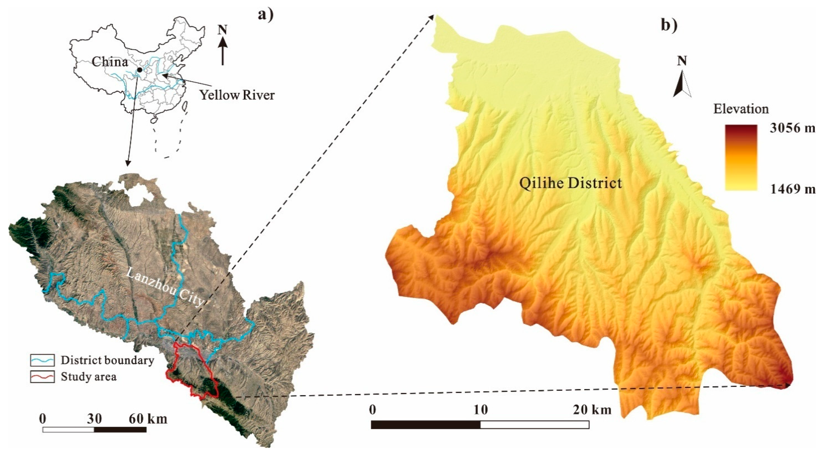
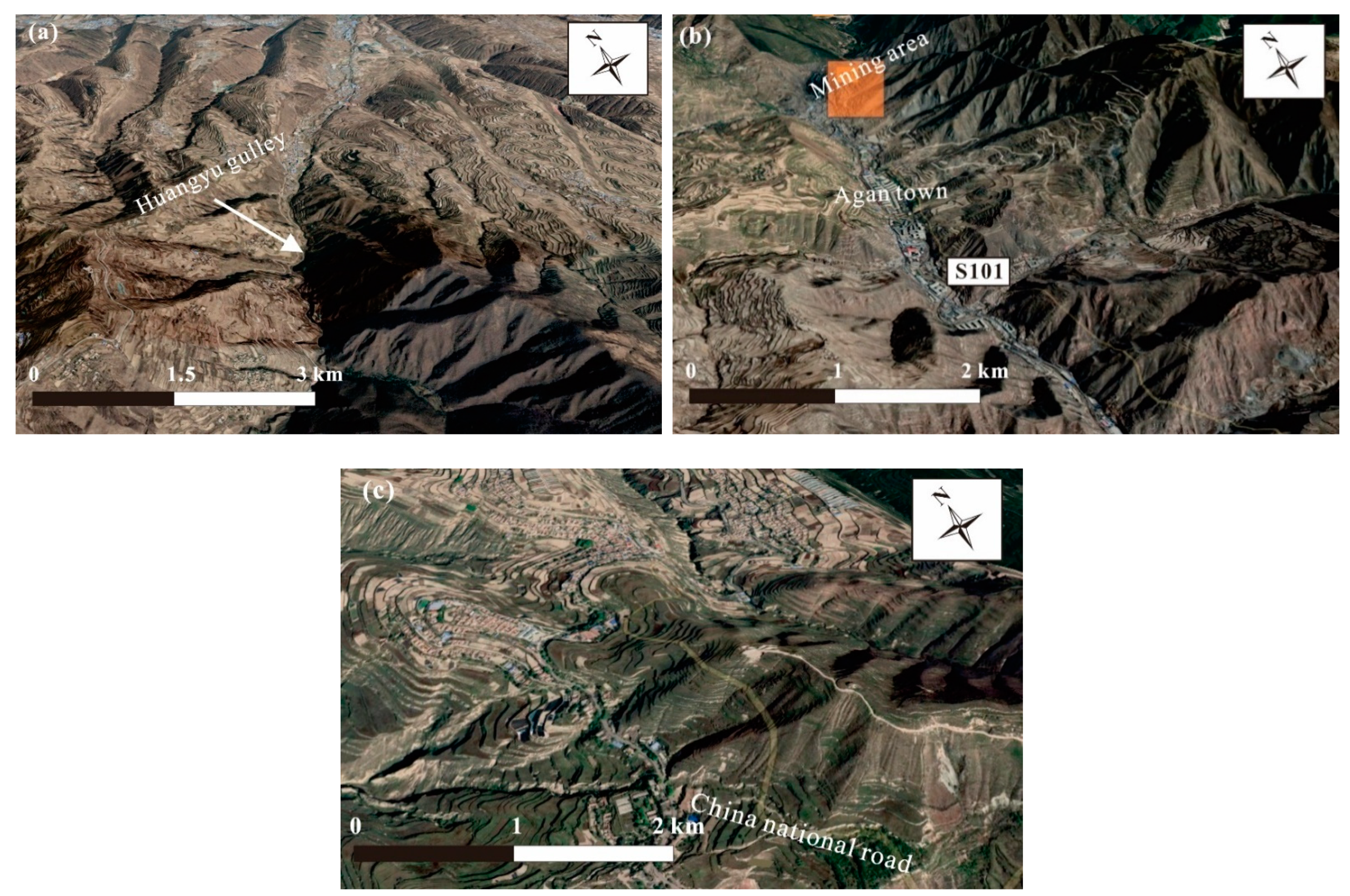
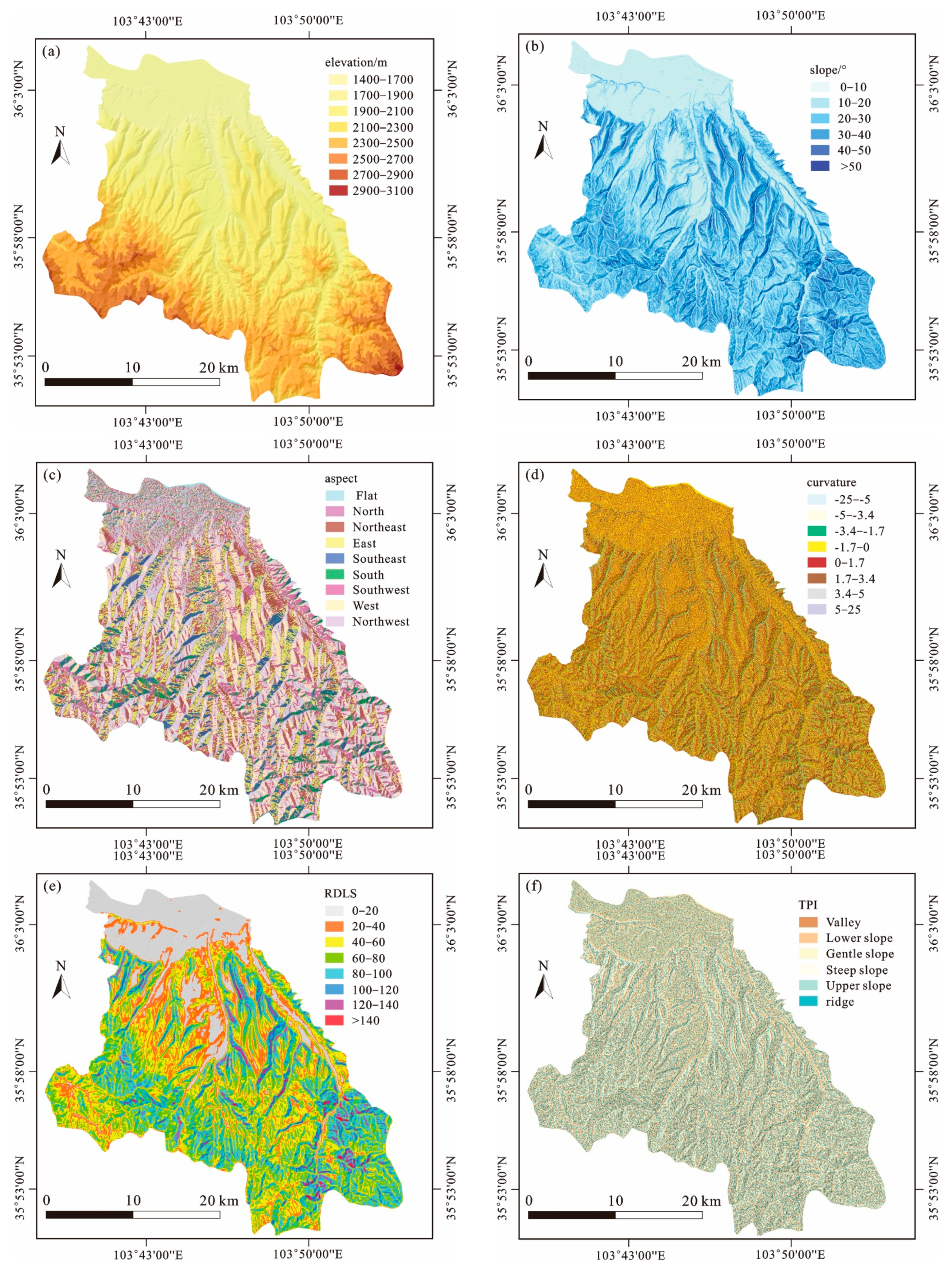
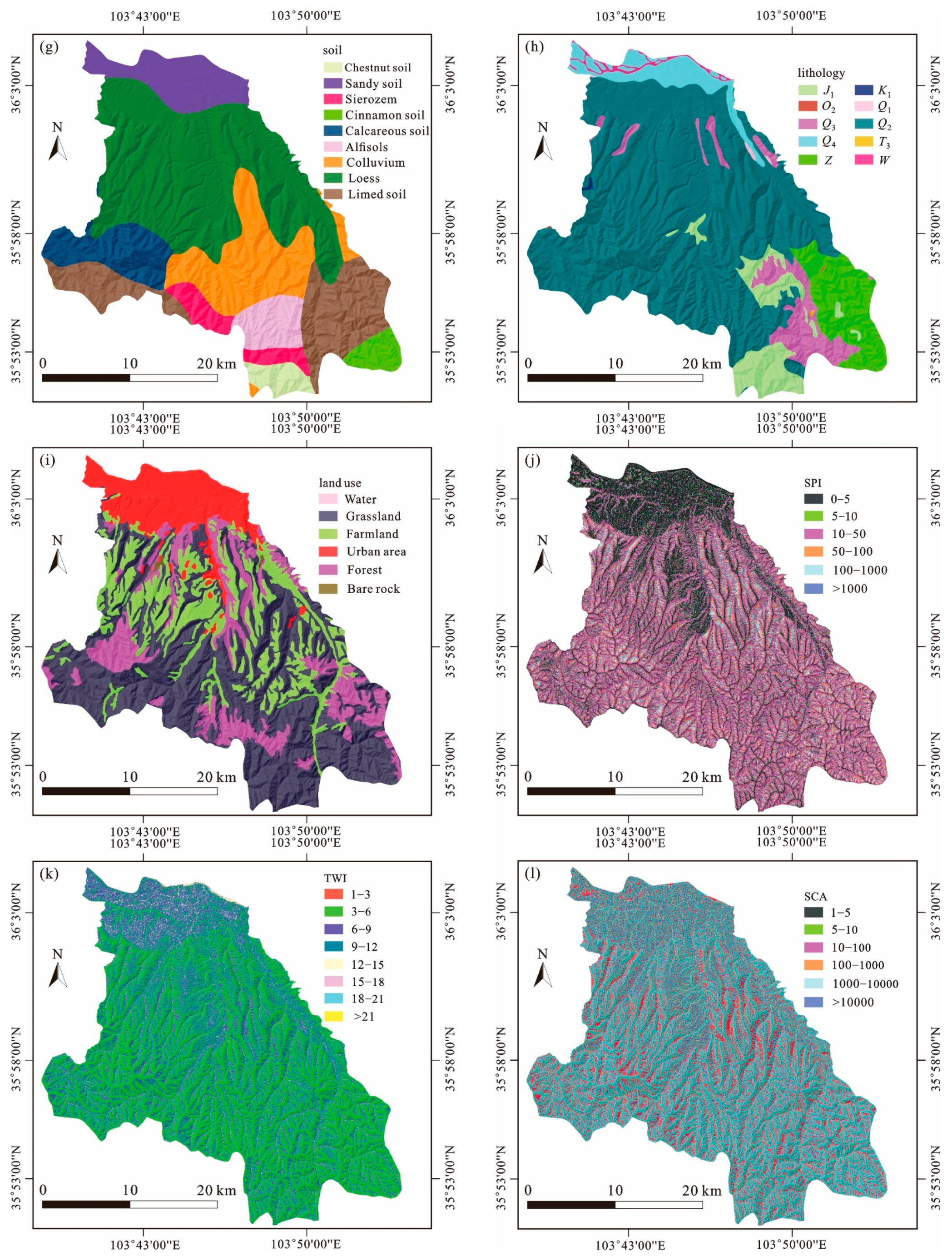
2.1. Description of the Study Area

The study area encompasses the Qilihe District (35°50′25″ N, 103°36′43″ E~36°06′09″ N, 103°54′28″ E) within middle–southern Lanzhou City, China, covering an area of 394.5 km² (Figure 1). The area is part of the western Longzhong Loess Plateau, which is highly dissected and lies within the Yellow River valley belt. It is characterized by a parallel ridge-and-valley area and surrounded by a typical hilly and mountainous landscape [41]. The elevation in the region ranges from 1469 to 3056 m above sea level, with high south and low north. The area has a temperate continental climate with a mean temperature of 7.8 ℃ and an average yearly rainfall of more than 327 mm. Meanwhile, a clear temporal difference on rainfall pattern can be seen: the dry season extends from November to March whereas the rainy season is between May and September, which normally yields a maximum total precipitation in August [41].

Two geological units can be observed in the region, namely the Lajishan and the Middle of Qilian strata. Both units have subhorizontal layering and several sets of subunits vertically. The exposed sedimentary strata include the Middle Ordovician (O₂), Sinian (Z), Upper Triassic (T₃), Lower Jurassic (J₁), Lower Cretaceous (K₁) and Quaternary (Q₁, Q₂, Q₃, Q₄). The most important difference among these strata is the lithology, of which the Gaolan Formation rock mass is the most common in the area. It has been subjected to the composite action of multistage regional metamorphism, magmatic activity, and geological structure. The lithologies are mainly schist, gneiss, variegated conglomerate, and quartzite. The other typical stratum is the Quaternary that can be represented by argillaceous pebble in the Qilihe faulted basins and by extensive loess deposits, which cover the bedrock with the thickness of more than 5 m in most situations. Most faults are distributed in the southern part of the region, extending from northwest to southeast, but the scales are moderate or small.

The resident population in the area is approximately 5.78 × 10⁵ inhabitants and the settlements are mainly distributed on the banks of rivers and within valley areas, especially the northern and southeastern parts. With a population density of more than 1300/km², this part of the district is highly populated and urbanized, where many engineering activities have been performed, such as infrastructure construction and farming [42].

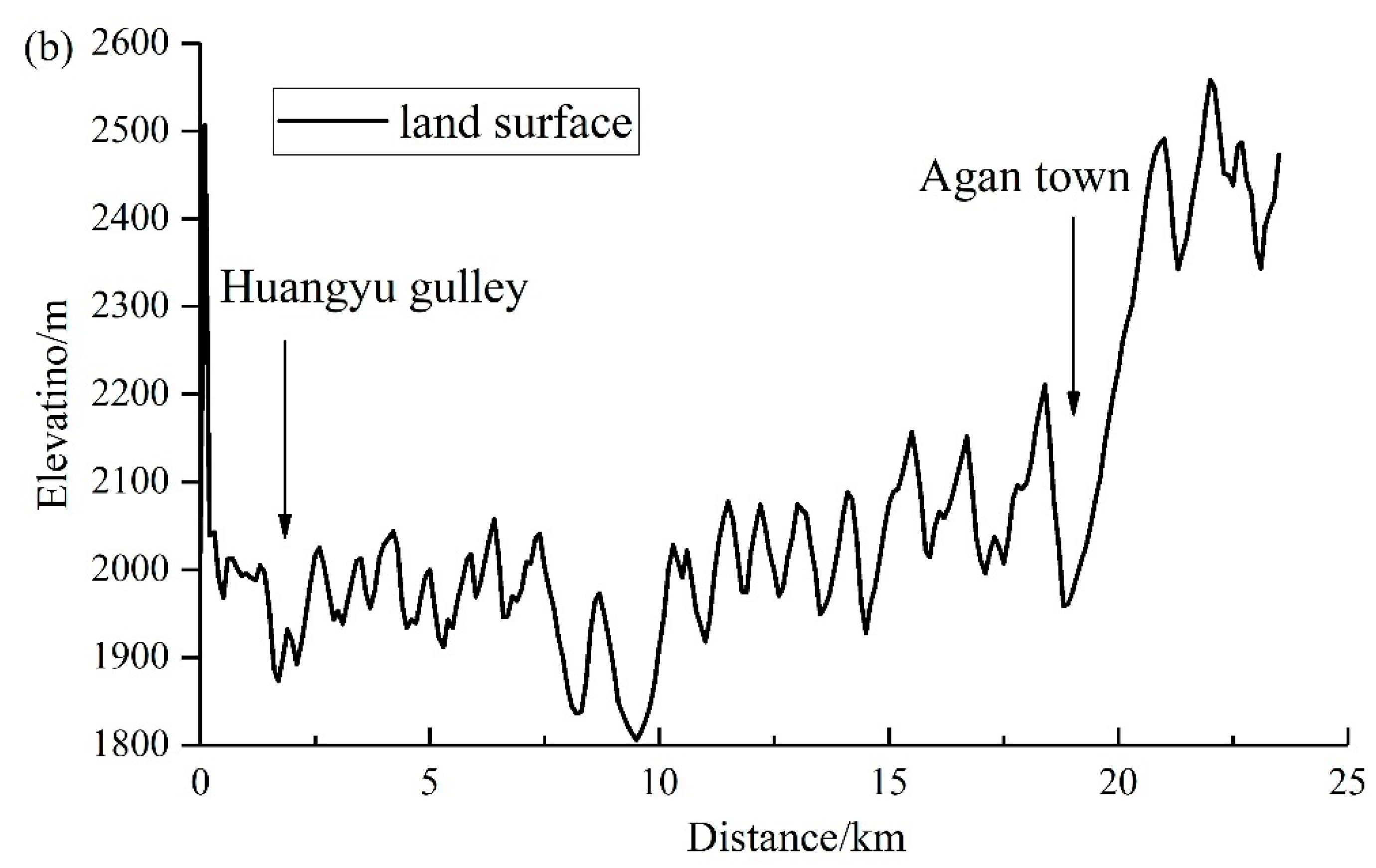
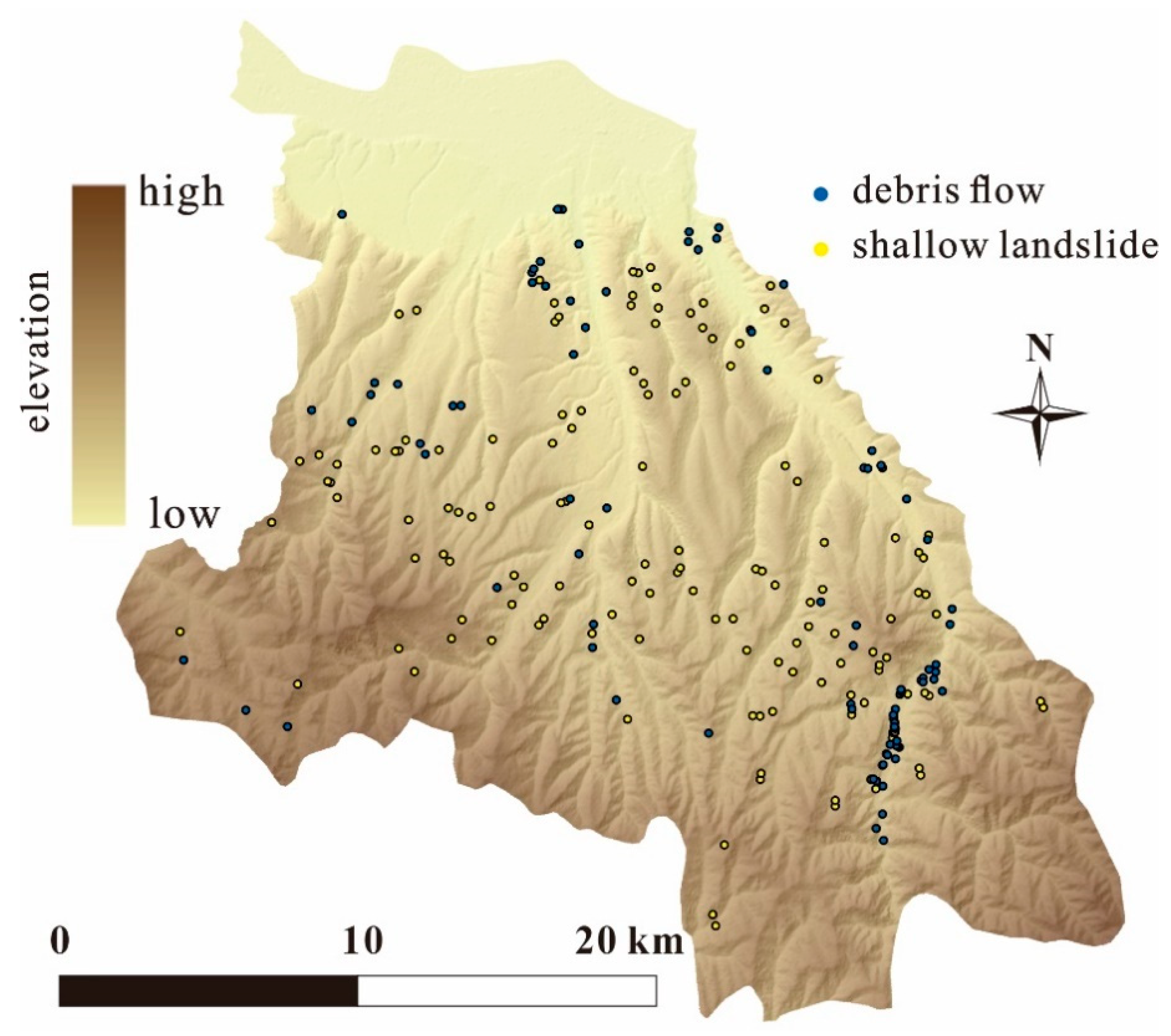
2.2. Landslide Inventory

Qilihe District spreads over a mixture of hilly and mountain landscape. Combined with the seasonal rainfall regime, interesting dynamics and plenty of landslides have been recorded in the region. The depths of these landslides vary from approximately 1 m to more than 20 m. Most of the landslides occurred in the loess deposits. Showing the spatial locations of these landslides in a GIS platform and creating an accurate database are important for LSA [43]. However, detailed detection of landslide extent is a rather complicated and challenging task. In this study, therefore, the landslide inventory was created according to an extensive field survey, earlier geotechnical reports, and previous literature [41]. Some literature [25,37] was referred to when we prepared the inventory to include some necessary information. The geotechnical reports were internal documents from the Lanzhou Institute of Geological Environment Monitoring in 2015. The details of every landslide were reported, such as area, volume, and type. It should be stated that landslides in these reports included the landslides that caused losses during 1996–2015. Landslides without losses are not included in the inventory; this is because there are very few and it is difficult to record when they occurred a long time ago. The field survey was conducted in 2017 and 2018, and we cross-checked the landslide information with that in the reports. The type of each landslide was confirmed according to protocol reported in standard literature [44,45].

Finally, a total of 227 landslides were recorded in the inventory, with an area of approximately 1.4 × 10⁶ m², accounting for 0.35% of the whole study area. Landslide volume varies greatly, with sizes ranging from 50 m³ to approximately 1 × 10⁶ m³. They can be roughly divided into three categories (Figure 2): (i) small-scale landslides in a rotational or translational form, most of which are associated with the upper soil layer; (ii) a small amount of rock slides or earth slides; and (iii) debris flows or earth flows in gulley channels. Additionally, there are also three large deep-seated landslides in the study area. However, the number is too few to fit with the sampling standard of statistical methods. Hence, they were not considered in the analysis. According to the depth of sliding surfaces, landslides in categories (i) and (ii) are shallow landslides, whereas category (iii) generally does not have evident sliding surfaces. From the perspective of movement type, most landslides in categories (i) and (iii) moved in the horizonal direction along the sliding surfaces or channels, whereas landslides of category (ii) had a larger vertical movement distance. Landslides of category (ii) and (iii) normally occurred during a short time so their impact forces were larger. However, because the number of buildings and people in their runout paths were small, the direct losses caused by these two categories of landslides were not very large. Some landslides of category (i) were characterized as creep deformation, which might show sudden acceleration behavior, particularly during the rainy season. Although the infrastructure affected by them was not totally destroyed, the increasing deformation of these landslides might pose a considerable risk to residents and properties.

During the next stage, the spatial distribution of these landslides was plotted on a 1:50,000 map with 12.5 m resolution in GIS. As seen in Figure 3a, this study shows landslide locations in the form of point shapefile in GIS. However, the polygon-based file of landslides is also available, which indicates the extent of each landslide. In addition, the detailed properties of individual landslides were linked and recorded in the database, such as the area, volume, occurrence time, and associated damage.

3. Methods

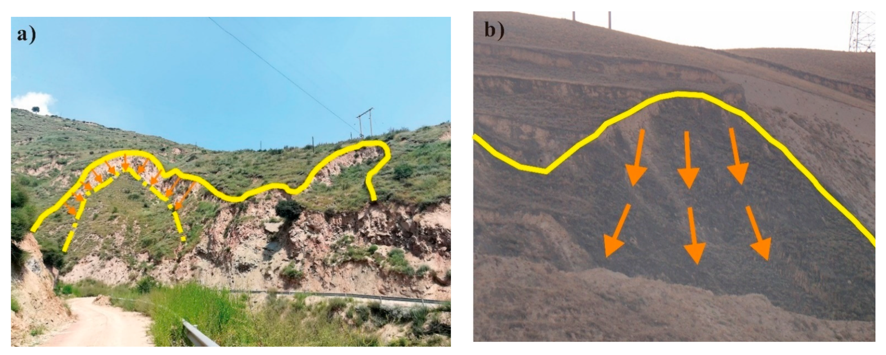
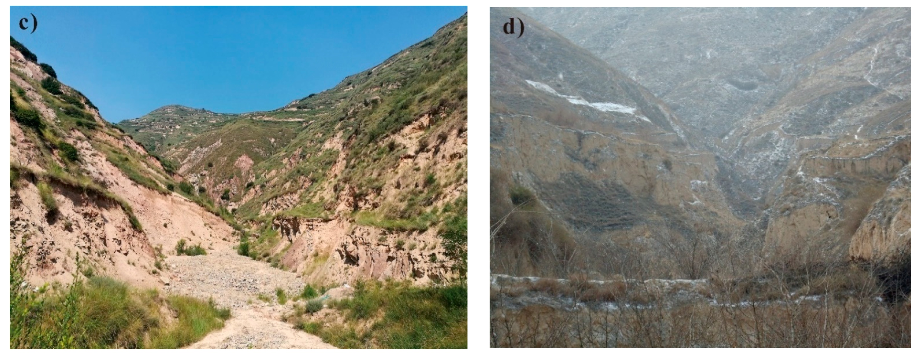
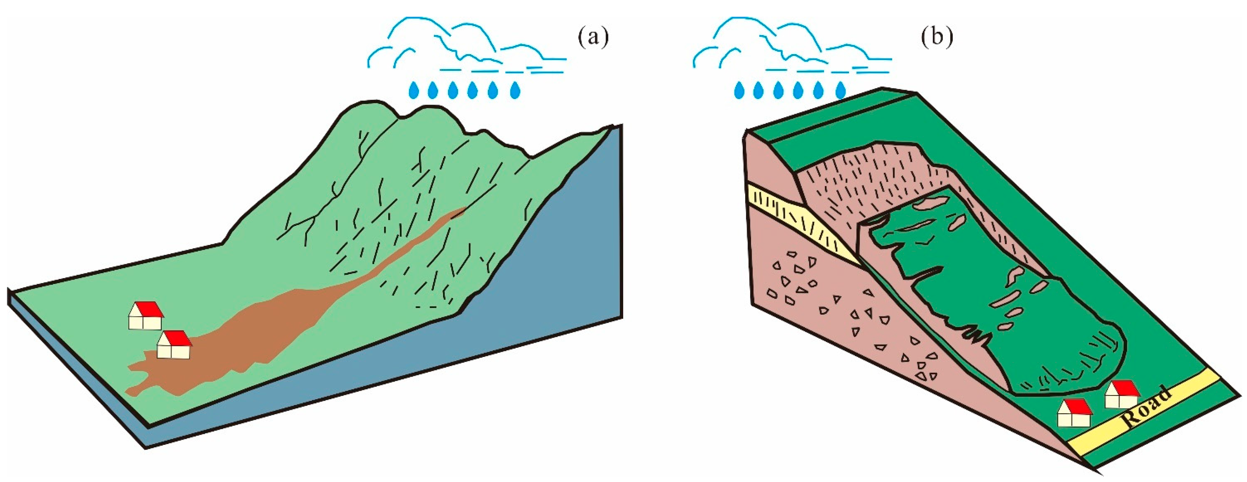
3.1. Landslide Typology

The main objective of this section is to justify why and how we divided the landslides in the inventory into different types. We analyzed the spatial distribution of landslides and clarified the difference of characteristics between different landslide types. According to this, we summarized the schematic models for different landslide types. Additionally, this analysis helps to understand the roles of factors in different landslide types.

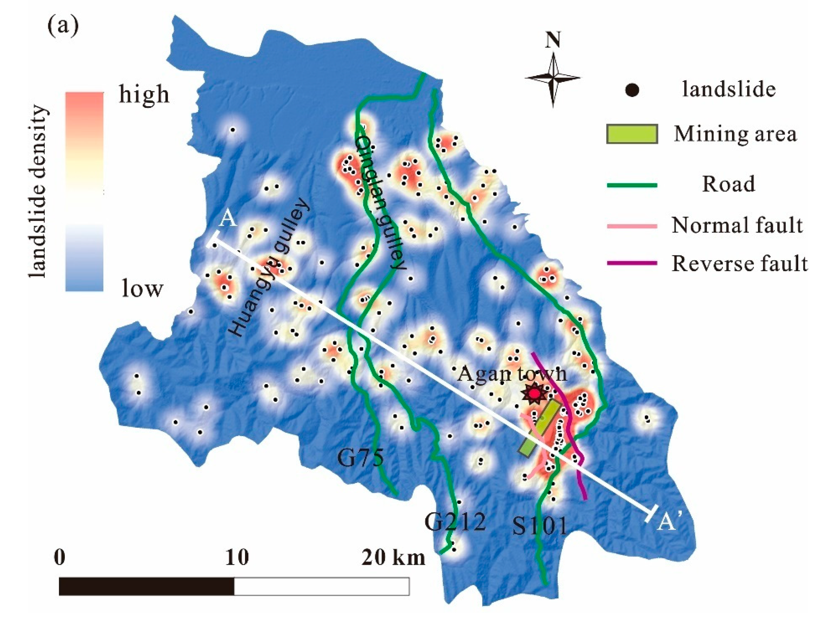
3.1.1. Analysis of Landslide Density

During this step, all of the landslides were projected onto the DEM according to their coordinates. The kernel density analysis tool in GIS was used to obtain the spatial density distribution of these points. As seen in Figure 3a, there are three areas in Qilihe District where landslides are densely distributed: (i) The northern part of the area—the Qinglan gulley and Leitan River are located in this area. On one hand, the long channel of the gulley provides a runout path for landslides [46]. On the other hand, the erosion of riverbanks also affects the slope stability [47]. (ii) The middle–western part of the area—as the largest gulley of the study area, Huangyu gulley is located here (Figure 3b), and it is one of representative areas prone to debris flows in the Qilihe District. (iii) the southeastern part of the area—this lies near Agan town, which is a highly populated region.

From the perspective of geological conditions and triggering factors, the study area has dozens of gullies and many have a long and steep channel. For instance, Huangyu gulley has the channel with a length of more than 3 km, and the elevation difference between the top and the bottom points reaches hundreds of meters. The loess and other Quaternary deposits in the mountain can be easily destabilized during the heavy rainfall and then form debris flows that move along the channel. In the southeastern part of the area, geological structures, particularly faults, are relatively concentrated. Most are parallel and have a direction from NW to SE. Historically, frequent tectonic movements make the rock–soil masses here relatively weak. Moreover, the strata angles are large at both sides of the faults. Nearby Agan town, there is a coal mine that has operated for more than ten years and greatly affects stability conditions of slopes. Meanwhile, a national road also passes this area. The frequent engineering activities—building construction, roads and mining activities—have caused many shallow landslides in the area. Moreover, Agan town is located in a gulley that also has a large elevation difference and steep slopes, so many debris flows have also occurred in this area, similar to the Huangyu gulley. Hence, the combined influences of internal geological conditions and external triggers make the Agan town area the most susceptible to landslides.

According to remote sensing images, the difference of geomorphology in different parts of Qilihe District can be observed. There are many gullies with different scales in the study area that extend from the south to north. As seen in Figure 4a,b, the cutting effect of gullies creates channels and steep slopes which are prone to debris flows. However, in the northern and eastern parts of the Qilihe District (Figure 4c), the topography is relatively gentle, and typical gullies and channels are very few. Roads and settlements are mainly located in this region; thus, external conditions are positive for shallow landslides.

3.1.2. Landslide Typology and Schematic Model

As mentioned above, according to topography conditions, triggering factors, and movement characteristics, the landslides in Qilihe District were divided into two types: shallow landslides and debris flows. Using the archived reports, pictures of the sites, and remote sensing images, the reclassification for every landslide was performed. As seen in Figure 5, the typical schematic models for two types of landslides in the study area are summarized. Although the materials composing of the sliding body may vary, the initiation of landslides is considered to be mainly controlled by the morphology. An important reason for this classification is the landslide mechanism, which may lead to different responses of landslides to the same influencing factor. Hence, it is not reasonable to use just one set of influencing factors for the susceptibility analysis of all the landslides. According to this rule, two types of landslides are shown in Figure 6. In total, there are 141 shallow landslides and 86 debris flows.

3.2. Weighted Frequency Ratio Model

Landslide susceptibility can be obtained by the weight of factors and rating of categories. As Lee et al. [38] reported, the weight shows the relative importance among factors (e.g., slope and lithology) whereas the rating represents the relative importance among categories of one factor (e.g., slope of 0~10° and 10~20°). In this study, the rating was determined by an index called frequency ratio and the weight of factors was calculated by a logistic regression model combined with a fuzzy analytical hierarchy process (FAHP) model.

3.2.1. Frequency Ratio Method

Frequency ratio is a kind of statistical index that can show the nonlinear relationship between landslide distribution and external factors. Generally, the statistical models are conducted based on the assumption that future landslides will occur under the similar/same conditions as past landslides [11,13]. The frequency ratio (FR) can be obtained as follows:

$$FR=\frac{\raisebox{1ex}{$L_i$}\!\left/ \!\raisebox{-1ex}{$TL$}\right.}{\raisebox{1ex}{$S_i$}\!\left/ \!\raisebox{-1ex}{$TS$}\right.}$$

(1)

where i is the ith category of one factor, L_i is the area of landslides within this category, TL is the total area of landslides in the entire study area, S_i is the area of ith category and TS is the total area of the factor (same with the total area of the study area). If FR is more than 1, the ith category is positive for landslide occurrence when compared to the average level of all categories for this factor. The larger the value of FR, the contribution given by this category is larger.

3.2.2. Calculation of Weight of Factors

An analytic hierarchy process (AHP), recognized as a useful technique for multiple criteria decision-making, has been widely employed in GIS-based susceptibility analysis. However, from the detailed descriptions on AHP in previous literature [29,48,49], the model semiquantitatively determines the weights of factors by comparing them in pairs, which is highly subjective. Hence, in this study fuzzy theory was integrated with AHP (called FAHP) that allows users to change the pairwise comparisons to fuzzy numbers in the judgment matrix [50,51]. The fuzzy judgment matrix $\tilde{A}$ can be expressed as follows:

$$\tilde{A}=\left[\begin{array}{llll}\tilde{1}& {\stackrel{}{\tilde{a}}}_{12}& \dots & {\tilde{a}}_{1n}\\ {\stackrel{}{\tilde{a}}}_{21}& \tilde{1}& \dots & {\tilde{a}}_{2n}\\ ⋮& ⋮& \ddots & ⋮\\ {\tilde{a}}_{n1}& {\tilde{a}}_{n2}& \dots & \tilde{1}\end{array}\right]$$

(2)

where n is the total number of factors. ${\tilde{a}}_{ij}$ is the fuzzy comparison value of ith factor compared with jth factor (i = 1, 2, … n; j = 1, 2, …n). If the ith factor is relatively important, ${\tilde{a}}_{ij}$ is set as 1 whereas ${\tilde{a}}_{ij}$ is 0 when the jth factor is more important than the ith factor. If both are of equal importance, the fuzzy comparison value is 0.5. The fuzzy geometric mean of every factor (${\tilde{\mathit{r}}}_i$) can be determined according to the geometric mean technique as follows:

$${\tilde{\mathit{r}}}_i={({\stackrel{}{\tilde{a}}}_{i1}\otimes {\stackrel{}{\tilde{a}}}_{i2}\otimes {\stackrel{}{\dots \otimes \tilde{a}}}_{in})}^{(1/n)}$$

(3)

The matrix $\tilde{A}$ can be converted into fuzzy consistent matrix $\tilde{E}={\tilde{e}}_{ij}(n\times n)$ as follows:

$${\tilde{e}}_{ij}=\frac{{\tilde{\mathit{r}}}_i-{\tilde{\mathit{r}}}_j+1}{{\tilde{\mathit{r}}}_j-{\tilde{\mathit{r}}}_i+1}$$

(4)

where ${\tilde{e}}_{ij}$ is the element in the matrix $\tilde{E}$, ${\tilde{\mathit{r}}}_i$ and ${\tilde{\mathit{r}}}_j$ are fuzzy geometric means of ith and jth factor, respectively. The matrix $\tilde{E}$ can be used to define the initial values of weights ${\tilde{W}}^{(0)}$:

$${\tilde{W}}^{(0)}={({\tilde{w}}_1,{\tilde{w}}_2,\dots {\tilde{w}}_n)}^T=\left[\frac{{\displaystyle \sum _{j=1}^n{\tilde{e}}_{1j}}}{{\displaystyle \sum _{i=1}^n{\displaystyle \sum _{j=1}^n{\tilde{e}}_{ij}}}},\frac{{\displaystyle \sum _{j=1}^n{\tilde{e}}_{2j}}}{{\displaystyle \sum _{i=1}^n{\displaystyle \sum _{j=1}^n{\tilde{e}}_{ij}}}},\dots \frac{{\displaystyle \sum _{j=1}^n{\tilde{e}}_{nj}}}{{\displaystyle \sum _{i=1}^n{\displaystyle \sum _{j=1}^n{\tilde{e}}_{ij}}}}\right]$$

(5)

where ${\tilde{W}}^{(0)}$ is the matrix composed of the initial values of weights (${\tilde{w}}_1,{\tilde{w}}_2,\dots {\tilde{w}}_n$). This matrix can also act as the initial vector of characteristic value ${\tilde{H}}_0={({\tilde{h}}_{01},{\tilde{h}}_{02},\dots ,{\tilde{h}}_{0n})}^T$. Then an iterative method can be adopted to obtain the characteristic vector ${\tilde{H}}_k$ as follows:

$${\tilde{H}}_k=\tilde{E}{\tilde{H}}_{k-1}(\mathrm{k}=1,2\dots \mathrm{n})$$

(6)

When the difference of ${\tilde{H}}_k$ and ${\tilde{H}}_{k-1}$ is less than ε (the accuracy determined by users), the vector obtained from the normalization of ${\tilde{H}}_k$ can be considered as the weight of factors.

As seen from the process mentioned above, a key step in the FAHP model is the determination of fuzzy number in the fuzzy matrix. However, the judgment of relative importance among factors is still necessary for this step, which is generally conducted by the expert-based method.

In this study, a logistic regression model was employed to rank the importance of factors quantitatively to remedy this limitation.

The logistic regression model considers landslide occurrences as a bivariate variable, i.e., only two values are used to express a landslide-related event: 0 and 1 represent the landslide presence and absence, respectively. If the influencing factors are set as independent variables and the landslide event is the dependent variable, the relationship between them can be given as:

$$Y=a_0+a_1{X}_{1j}+a_2{X}_{2j}+\cdot \cdot \cdot +a_n{X}_{nj}$$

(7)

where Y is the landslide event, X are the influencing factors, X_nj represents the jth category of nth factor. The values from a₀ to a_n are regression coefficients of these factors. Because a larger/smaller coefficient can lead to a value closer to Y = 1/0, these coefficients can be considered as an index showing the importance of a factor [21]. It should be noted that a factor can have both negative and positive effects on landslide occurrence, thus the importance is determined by the absolute values of coefficients and not the actual values.

4. Data Preparation and Analysis

4.1. Analysis of Influencing Factors

Multiple factors may influence the landslide occurrence and they are often interconnected [52]. Therefore, determination of influencing factors is an essential step for landslide susceptibility mapping because researchers need to extract principal information that can represent landslide mechanisms. According to previous work and expert knowledge [8,53,54], a total of 12 influencing factors are utilized as preliminary inputs in the present analysis, which can be divided into five categories: (i) geomorphological factors, including elevation, slope, aspect, curvature, relief degree of land surface (RDLS), and topographic position index (TPI), (ii) the geological factor, lithology, (iii) hydrological factors, including stream power index (SPI), topographic wetness index (TWI), and specific catchment area (SCA), (iv) land use, which is an environmental factor that can be anthropically modified, and (v) soil. It should be noted that some factors have been widely accepted by scientific communities in this topic (e.g., slope and lithology) while some are not commonly used in this topic, such as RDLS and SCA. However, they are truly related to some aspects of landslides, such as mechanical and hydrological processes. Additionally, some factors are considered more as triggering factors of landslides instead of influencing factors because they generally have evident temporal variability. For example, both rainfall and human activities have impacts on landslides, but they can change much dynamically even during short periods. Therefore, they influence the temporal distribution of landslides more than spatial distribution [55,56], which excludes them from the database.

The multicollinearity analysis of factors was carried out before the calculation [57]. An ArcGIS tool named “Band Collection Statistics” was applied to do this. The results showed that the correlation between every two factors is not larger than 0.4. Hence, the collinearity among factors is considered appropriate. These selected factors involve both continuous and categorical data, of which the former may increase the computational amount much and subsequently lead to complex data processing. To remedy this, these factors were discretized into several categories with the same attribute interval (Figure 7). A review of the literature [15,20,58,59] showed that an attribute number of 5~9 is reasonable because it not only simplifies the calculation but also leads a moderate division of continuous data. The main reasons to select these factors and descriptions regarding reclassification are clarified below.

Elevation

Elevation normally represents the potential energy of a slope and it also impacts the environmental conditions on slopes such as human activity, vegetation, and climate. The digital elevation model (DEM) of the study area was obtained from free open-source data (http://www.gscloud.cn/ accessed on 25 October 2020). The resolution selected was 12.5 m because its ability in quantitative analysis of geomorphological processes has been proven [60]. The elevation in the area varies from 1469 m to 3056 m a.s.l. and was classified into eight classes with an interval of 200 m (Figure 7a).

Slope

Slope reflects the steepness at each grid surface, which contributes much to slope stability. The slope map was prepared from the DEM in GIS, which shows a range from 0 to 74°; 10° was used as the interval [61] and a total of six classes were obtained (Figure 7b).

Aspect

Aspect represents the direction that a slope faces. This factor causes differences in microclimate (e.g., temperature and sun exposure) and affects land use on slopes. The aspect map (Figure 7c) was created from the DEM map. Eight directions (i.e., north, northeast, east, southeast, south, southwest, west, and northwest) were determined based on aspect values, in addition to flat area (the value is −1).

Curvature

The curvature controls the flow across a surface, thus affecting the erosion and deposition. The standard curvature was used in this study, which considers both the plan and profile curvatures [62]; thus, the whole process of flow can be understood accurately. The curvature values in the area range from –25 to 24 and divided into eight classes [63,64], among which most cells distribute in the range from −5 to 5 (Figure 7d).

Relief Degree of Land Surface

RDLS is an indicator to describe the topographic characteristics of the region, which can be obtained by calculating the maximum difference in height per unit area [65]. The map created shows that RDLS values within the study area vary from 0 to 169, which were divided into eight classes (Figure 7e).

Topographic Position Index

TPI has an impact on landslide susceptibility because many physical processes on the slope are highly associated with topographic position [66,67]. The map was created using the Land Facet Corridor Designer (LFCD) (http://www.jennessent.com/arcgis/land_facets.htm accessed on 26 October 2020) extension in ArcGIS 10. There are six classes in this factor: valley, lower slope, gentle slope, steep slope, upper slope, and ridge (Figure 7f).

Soil

The soil herein mainly represents the materials overlying bedrock, which also makes up the sliding bodies of landslides. Geotechnical parameters are quite different when soil type varies, which can greatly affect the slope stability. Because the barren area (e.g., bare rock area) are limited in the Loess Plateau, most areas are covered by various sediments. Obtained from the Resource and Environment Science and Data Center (RESDC) (http://www.resdc.cn/Default.aspx accessed on 26 October 2020) of China with a 1:1,000,000 scale, the soil data were reclassified into nine types (chestnut soil, sandy soil, sierozem, cinnamon soil, calcareous soil, alfisols, colluvium, loess, limed soil) in the study area, among which loess and colluvium are the most widely distributed (Figure 7g).

Lithology

The lithology can represent the geomechanical and hydraulic properties of the bedrock and subsequently affects the soil coverage [37]. Hence, it is accepted that the lithology is one of the most representative factors for landslide occurrence. This factor was obtained from geology maps (scale 1:100,000) provided by Lanzhou Institute of Geological Environment Monitoring. The geological units were divided into nine categories based on their formation ages (Figure 7h): Middle Ordovician (O₂), Sinian (Z), Upper Triassic (T₃), Lower Jurassic (J₁), Lower Cretaceous (K₁), and Quaternary (Q₁, Q₂, Q₃, Q₄).

Land Use

Land use affects the root cohesions and hydrological process on the landscape, and also indirectly explains the human influences on the hillslopes [68]. A land use map of 2018 downloaded from RESDC (http://www.resdc.cn/Default.aspx accessed on 28 October 2020) including six classes (grassland, farmland, urban area, forest, water, and bare rock) was created in 1:100,000 scale (Figure 7i).

Stream Power Index

Runoff is one of the most important hydrological processes during the landslide events, among which some factors are key indicators for runoff models. SPI can measure the erosive power of flowing water based on slope and contributing area. It can be calculated by the following equation:

SPI = ln (DA × tan (G))

(8)

where DA is the upstream drainage area at a given cell and G is the slope value at this cell. This map was generated by the raster calculator tool in ArcGIS 10 (Figure 7j).

Topographic Wetness Index

TWI (Figure 7k) considers both slope and local upslope contributing area, which can be used to quantify the topographic attributes of hydrological processes [69]. The equation to calculate this index is expressed as:

TWI = ln (a/tan β)

(9)

where a is the upslope area draining from a specific cell and tan β is the slope at this cell.

Specific Catchment Area

SCA is defined as the upstream catchment area of a given unit [70], which is a parameter commonly used for hydrology and soil erosion modeling (Figure 7l). This factor reflects the area draining to the outlet of the catchment; thus, it can be determined as follows:

$$SCA=\underset{CL\to 0}{\lim }\frac{CA}{CL}$$

(10)

where the CA is the upstream area of a contour segment and CL is the length of the segment.

During the next stage, these factors were digitalized to corresponding thematic maps that were in raster format with 12.5 m-resolution cells. We used the band collection statistics tool in GIS to calculate the interrelationship among factors and the results showed that the correlation coefficient between every two factors was less than 0.4. This means these factors are independent variables when shown together.

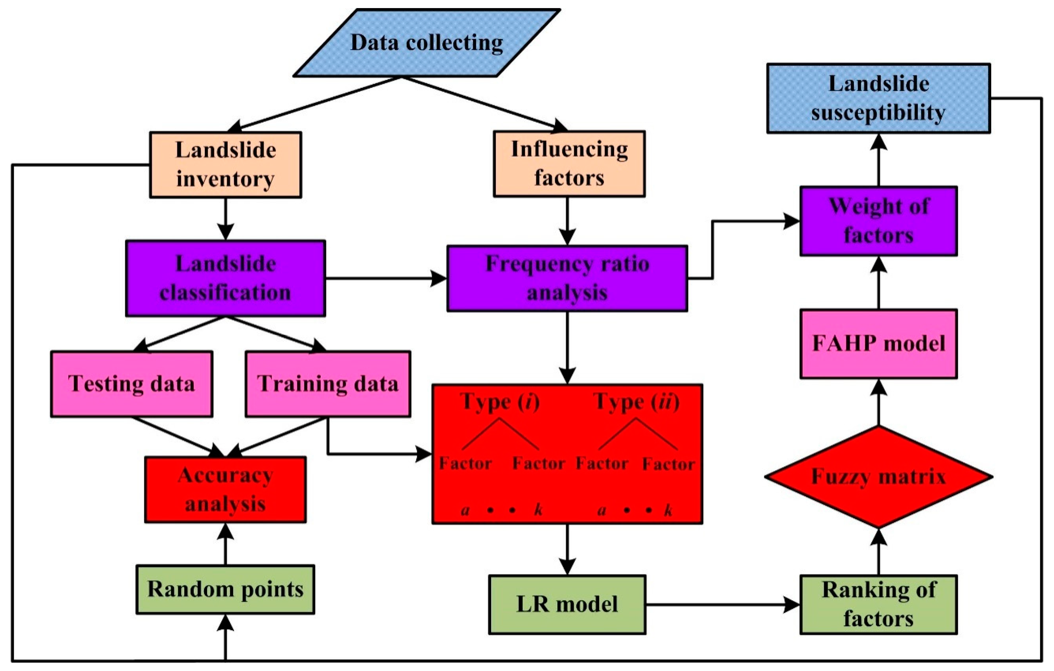
4.2. Procedure of Landslide Susceptibility Modeling

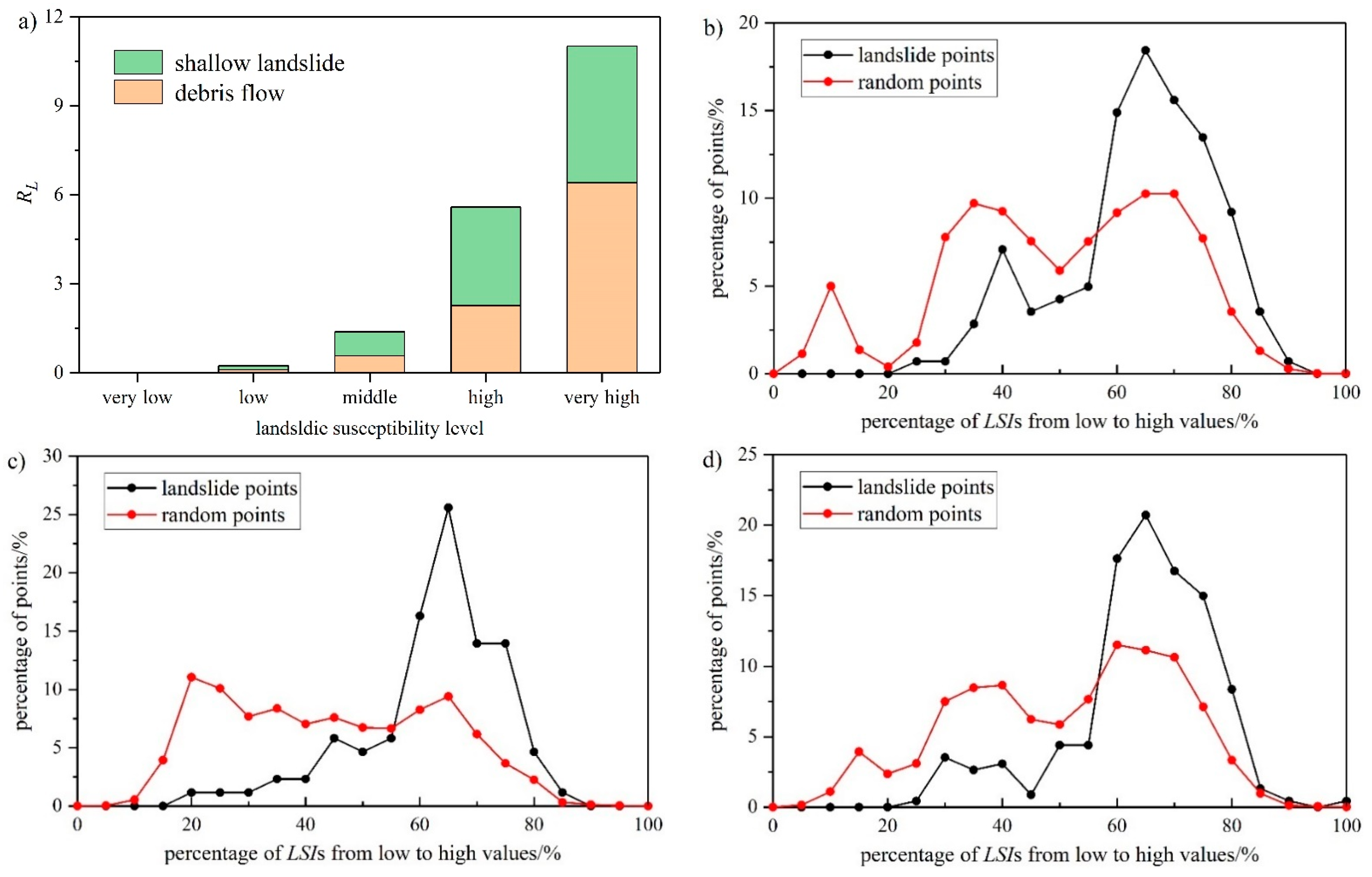
In this step, all landslide polygons were transformed to cells for the subsequent analysis of influencing factors. The entire area is characterized by a maximum row number of 2579 and column number of 2395 cells. The total number of cells is 2,599,948, among which 8978 cells cover landslides, including 6528 cells for shallow landslides and 2450 cells for debris flows. In the ArcGIS database, all influencing factors (including detailed values, category numbers and frequency ratios) were linked to the landslide inventory for application in the weighted frequency ratio model. The detailed procedure of this analysis is shown in Figure 8. These steps are described as follows:

(i) All of 8978 cells covering landslides were converted into a point shapefile. The same number of cells that do not cover landslides were randomly selected over the whole area. Eighty percent of the data (5222 cells covering shallow landslides and 1960 cells covering debris flows) were set as the training dataset, whereas the remaining 20% of the data (1306 cells covering shallow landslides and 490 cells covering debris flows) were the testing data. Similar with the frequency ratio analysis in Section 3.1, the preparation of the dataset was also individually conducted for each type of landslide, not for the entire landslide inventory. For a specific cell, a total of 13 attribute values were contained, i.e., 12 influencing factors and one set of bivariate data that represented the landslide presence/absence (0: absence; 1: presence). The influencing factors were set as input data whereas the bivariate data were the output data. Hence, the datasets used for modeling are shown in

Table 1. The datasets used in modeling.

Type of Data	Input Data	Description	Output Data	Description
Training data	F1(t-input)5222 × 12	Influencing factors of cells covering shallow landslides	F1(t-output)5222 × 1	Training points of shallow landslides
	NF1(t-input)5222 × 12	Influencing factors of cells without covering landslides	NF1(t-output)5222 × 1	Training points of nonlandslide area
	F2(t-input)1960 × 12	Influencing factors of cells covering debris flows	F2(t-output)1960 × 1	Training points of debris flows
	NF2(t-input)1960 × 12	Influencing factors of cells without covering landslides	NF2(t-output)1960 × 1	Training points of nonlandslide area
Testing data	F1(t-input)1306 × 12	Influencing factors of cells covering shallow landslides	F1(t-output)1306 × 1	Testing points of shallow landslides
	NF1(t-input)1306 × 12	Influencing factors of cells without covering landslides	NF1(t-output)1306 × 1	Testing points of nonlandslide area
	F2(t-input)490 × 12	Influencing factors of cells covering debris flows	F2(t-output)490 × 1	Testing points ofdebris flows
	NF2(t-input)490 × 12	Influencing factors of cells without covering landslides	NF2(t-output)490 × 1	Testing points of nonlandslide area

.

(ii) All of the training datasets were converted from a database in ArcGIS to numeric matrices and imported into SPSS Modeler software where the logistic regression method was employed to fit the equation of landslide occurrence.

(iii) The regression coefficients for every influencing factor obtained from step (ii) were considered as the relative importance. A fuzzy matrix was determined according to Equation (2) and subsequently used in the FAHP model. The model was performed in Stata software where a self-written program was applied and the weight of every influencing factor was determined from this step.

(iv) The steps noted above determined two kinds of weights: one is the weight of factors and the other is the rating of categories of each factor. Hence, the landslide susceptibility index (LSI) at one cell can be calculated as follows:

$$LSI={\displaystyle \sum _{i=1}^{11}{W}_i\times R_{ij}}$$

(11)

where LSI is the landslide susceptibility index at one cell; W_i is the weight of ith factor at this cell; and R_ij is the rating of jth category of the ith factor at this cell, which is expressed as the frequency ratio in this study. The values of LSI at all cells were ranked from high to low and divided into five intervals on average (i.e., equal interval method for classification), namely five landslide susceptibility levels: very high, high, middle, low, and very low. To obtain the susceptibility map for the entire inventory, the LSIs of two types of landslides were added, and the same classification method was used for susceptibility zonation.

(v) The validation of the model was determined by considering the area of each susceptibility level being different, not the landslide number or density, but the relative ratio of landslides (R_L) was counted to check the model performance. This index was defined as follows:

$$R_L=\frac{\raisebox{1ex}{$A_{Li}$}\!\left/ \!\raisebox{-1ex}{$T{A}_L$}\right.}{\raisebox{1ex}{$S_i$}\!\left/ \!\raisebox{-1ex}{$TS$}\right.}$$

(12)

where S_i is the area of one susceptibility level and TS is the total area of the study area; A_Li is the area of landslides in this susceptibility level; and TA_L is the total area of the landslides in the study area. Hence, this index inherently reflects the the ratio between the area proportion of one susceptibility level in the whole area and the proportion of landslides in the entire landslide inventory. If a model contains more historical landslides in less area, it has a higher value of R_L, which indicates better performance.

Additionally, the receiver operating characteristic (ROC) curve, which has been widely used in previous studies, was used to compare the performance of different models. The accuracy can be evaluated according to the area under the curve (AUC); the larger the AUC value, the greater the model accuracy.

5. Results

5.1. Weights of Influencing Factors

According to

Table 2. Description of influencing factors and frequency ratio of every category.

Factor	Category	Frequency Ratio
		Shallow Landslides	Debris Flows
Elevation/m	1400~1700	1.001	0.296
	1700~1900	2.579	1.958
	1900~2100	1.352	1.939
	2100~2300	0.190	0.877
	2300~2500	0.135	0.197
	2500~2700	0.102	0.007
	2700~2900	0	0
	2900~3100	0	0
Slope/°	0~10	0.827	0.224
	10~20	1.102	0.952
	20~30	0.784	1.270
	30~40	1.373	1.665
	40~50	2.663	2.557
	>50	0	3.528
Aspect/°	Flat area	0.172	0.011
	North	0.669	0.932
	Northeast	0.583	0.920
	East	1.976	1.033
	Southeast	0.707	0.643
	South	0.300	0.680
	Southwest	0.499	1.534
	West	1.199	1.276
	Northwest	1.151	0.933
Curvature	−25~–5	0.364	1.776
	−5~−3.4	1.684	1.497
	−3.4~−1.7	1.042	1.295
	−1.7~0	1.030	0.997
	0~1.7	0.947	0.891
	1.7~3.4	0.937	1.013
	3.4~5	1.017	1.259
	5~25	1.243	2.643
RDLS	0~20	0.417	0.056
	20~40	1.817	0.647
	40~60	0.921	0.894
	60~80	0.801	1.170
	80~100	1.601	1.761
	100~120	0.401	1.606
	120~140	0.181	2.430
	>140	1.739	1.632
TPI	Valley	0.453	0.596
	Lower slope	0.831	0.800
	Gentle slope	0.727	0.721
	Steep slope	1.232	1.124
	Upper slope	1.224	1.193
	Ridge	1.139	1.319
Soil	Chestnut soil	0	0.006
	Sandy soil	0.164	0
	Sierozem	0	0.232
	Cinnamon soil	0	0
	Calcareous soil	0	0.174
	Alfisol	0	0.162
	Colluvium	0.217	2.196
	Loess	1.862	1.495
	Limed soil	1.306	0.222
Lithology	J1	0.945	1.226
	K1	0	0
	O2	0	0
	Q1	0	0
	Q2	2.228	2.109
	Q3	0.948	0.945
	Q4	1.064	0.022
	T3	0	2.136
	Z	0.608	1.140
	Water	0	0
Land use	Water	0.642	0.947
	Grassland	2.085	1.311
	Farmland	0.734	0.008
	Urban area	1.065	1.620
	Forest	0	0
	Bare rock	0	0
SPI	0~5	0.812	0.527
	5~10	0.937	0.787
	10~50	1.006	1.054
	50~100	1.479	1.549
	100~1000	1.209	1.899
	>1000	0.483	0.901
TWI	1~3	1.406	1.692
	3~6	1.017	0.998
	6~9	1.052	1.094
	9~12	0.684	0.719
	12~15	0.377	0.308
	15~18	0.081	0
	18~21	0.313	0
	>21	0	0
SCA	1~5	0.871	0.639
	5~10	0.747	0.624
	10~100	0.969	0.941
	100~1000	1.236	1.452
	1000~10000	1.183	1.149
	>10000	0.267	0.742

, a same category may have different impacts on the two types of landslides. Taking the slope as an example, 10~20° slope value is positive for shallow landslide occurrence because the frequency ratio is more than 1.1. Although the range from 40° to 50° also has a large frequency ratio, our statistics showed the number of landslides in this range was small. This leads us to conclude that the lower slope values have a positive impact on this type of landslide. Although this does not fit with some previous studies that revealed medium slopes (e.g., 40°~60°) may contribute the most to landslides in hilly areas [68,71], it reflects well the distribution features of shallow landslides in this study area. For debris flows, most are distributed in areas with slopes of 30°~40° (frequency ratio 1.665), 40°~50° (frequency ratio 2.557), or 50°~60° (frequency ratio 3.528), which is different from the case of shallow landslides.

Regarding the RDLS, shallow landslides have the largest FR value at 20~40 (1.817) and 80~100 (1.601). Although the value of RDLS > 140 is also high, very few landslides occur in this region. This is different from that of debris flows. Most debris flows occur in the region with RDLS more than 80. This indicates that shallow landslides mainly occur in the region that is relatively flat, whereas debris flows mainly occur in variable terrain.

Regarding the aspect, shallow landslides mainly occur in the area with an eastern direction, whereas debris flows mainly occur in areas that have a southwest and west aspect.

Regarding the curvature, shallow landslides have larger FR values when the curvature is at −5~−3.4 and 5~25, whereas debris flows mainly occur where curvature is less than −3.4 or larger than 5.

Some similarities can also be observed on these two types of landslides. In the area with low elevations, both types have evidently larger frequency ratios than the area with higher elevations. Regarding the TPI, both types mainly occur in steep and upper slopes, which are normal situations.

Overall, from the frequency ratio of the different classes of factors, different conditions (mainly geomorphological) in which the two landslide types appear can be observed.

In addition to geomorphological factors, the impacts of other conditions can be seen. Taking the soil type as an example: the frequency ratio of loess and limed soil on shallow landslides are 1.862 and 1.306, thus indicating the these are positive conditions for shallow landslides. The frequency ratios of the other types are all less than 1. On the contrary, the frequency ratio on debris flows given by limed soil is rather low. This is also the case regarding lithology: the Lower Jurassic (J₁) and Sinian (Z) lithologies are negative for the occurrence of shallow landslides, while both lithologies are positive for debris flows. Such evident differences showed that the landslide typology is a major reason influencing the nonlinear relationship between factor and landslide development and occurrence. In contrast, some factors have similar influence on both types of landslides. For instance, the SCA ranging from 100 m² to 10,000 m² has the greatest influence on both types while a SCA greater than 10,000 m² is negative for landslide occurrence. This is mainly because flowing water mostly converts into runoff on slope surfaces rather than infiltration flow inside slopes when the upstream area is too large or under extreme rainfall events. Moreover, the depths of many landslides in the area are small; thus, the slopes may be already saturated when the flowing water increases significantly.

The result from the logistic regression model follows:

$$\begin{array}{l}{Y}_1=0.7824X_{1j}-0.749X_{2j}+0.6317X_{3j}+0.4517X_{4j}+1.022X_{5j}+0.6493X_{6j}\\ +1.383X_{7j}-0.9325X_{8j}+0.0267X_{9j}+0.4786X_{10j}+0.5111X_{11j}+0.5754X_{12j}-6.264\\ Y_2=0.9075X_{1j}+0.357X_{2j}+0.2103X_{3j}+0.0187X_{4j}+0.8169X_{5j}-0.0799X_{6j}\\ +1.14X_{7j}+0.4361X_{8j}+0.954X_{9j}+0.4622X_{10j}-0.1283X_{11j}+0.2693X_{12j}-6.682\end{array}\}$$

(13)

where Y₁ represents the shallow landslides and Y₂ is the debris flows. X₁~X₁₂ are elevation, slope, aspect, curvature, RDLS, TPI, soil, lithology, land use, SPI, TWI, and SCA, respectively. The j means jth category within a factor occurring at the calculated cell. According to Equation (13), the weight of every influencing factor calculated by FAHP model is shown in

Table 3. The ranking of importance of factors and their weights.

Factor	Ranking of Importance		Weight
	Shallow Landslide	Debris Flow	Shallow Landslide	Debris Flow
Elevation	4	3	0.104	0.128
Slope	5	7	0.086	0.059
Aspect	7	9	0.059	0.041
Curvature	11	12	0.026	0.021
RDLS	2	4	0.161	0.104
TPI	6	11	0.071	0.026
Soil	1	1	0.221	0.221
Lithology	3	6	0.128	0.071
Land use	12	2	0.021	0.161
SPI	10	5	0.033	0.086
TWI	8	8	0.049	0.049
SCA	9	10	0.041	0.033

.

It can be found that the weight of a same factor varies with the landslide typology. This illustrates that different types of landslides in an area are conditioned in different ways by the same set of influencing factors. The most relevant influencing factors to shallow landslides are soil, RDLS, and lithology, while those for debris flows are soil, land use, and elevation. There are two possible reasons why soil is important for both landslide types: one is because geotechnical properties vary with soil types, which can affect slope stability significantly; the other aspect is that this factor has impact on runoff processes and soil moisture on slopes. Shallow landslides can be easily triggered by heavy rainfall or human engineering activities when the soil properties (especially cohesion and friction angle) are weak. For debris flows, they are often related to the failure of a colluvial soil layer overlying the bedrock on hillslopes [46]. Most debris flows in the study area occur in the colluvium and cinnamon soil layers, which agrees well with the findings from some other regions [31,72]. It is evident that the factor contributes much when landslides mainly distribute on a certain category within a factor. From the perspective of spatial location, most shallow landslides are located along the road lines or coal mines; thus, easily excavated lithology is also relatively important.

For debris flows, many are located on medium-height (1700~2300 m) hillslopes with the frequency ratio more than 0.8, where sufficient potential energy and material sources are present. On the contrary, the high mountain areas (2300~3100 m) have very few landslides and their frequency ratio (less than 0.2) is evidently lower than that of medium-height mountains. Hence, the distribution of debris flows vary with elevation by a large level and this factor shows great importance. Regarding land use, the result on its importance is similar to some studies in other mountainous settings, which concluded that the initiation and flow dynamics (e.g., infiltration and runoff) during this type of landslide event have a strong relationship with vegetation types on the slope. For instance, Shu et al. [68] analyzed the landslide density in a debris-flow-prone area of the Pyrenees Mountains, and found that the land use types and land cover change have a great impact on landslide susceptibility. However, most shallow landslides in the study area were triggered by human activities, so the number of shallow landslides involved in farmland and urban area are more than that of debris flows. The computed result on frequency ratio (Table 2) agrees well with this point; the frequency ratio of farmland for shallow landslides reaches 0.734 while it decreases to 0.008 (almost no landslides in this category) for debris flows. Therefore, the concentrated distribution of landslides leads to a relatively high weight of this factor.

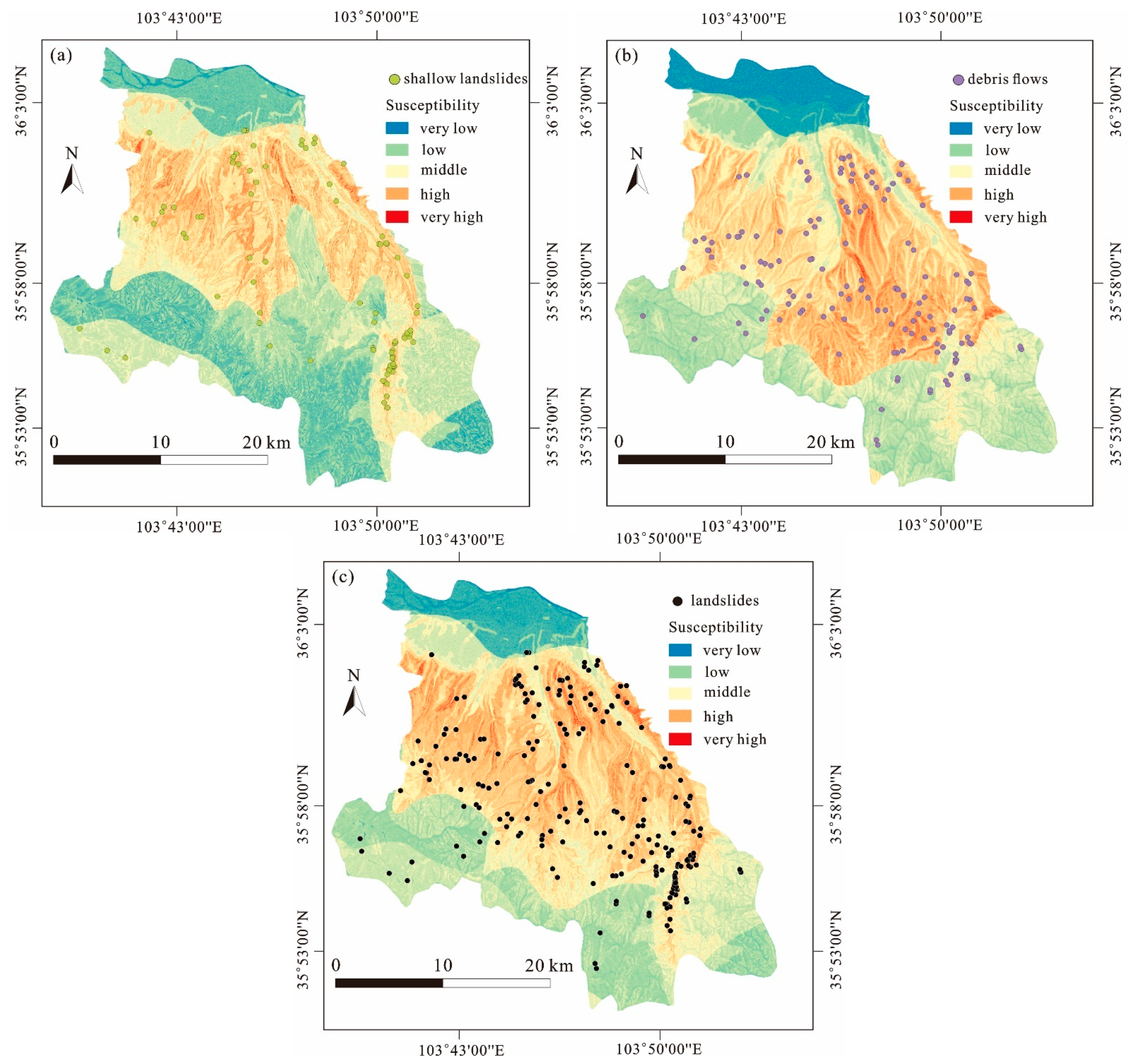
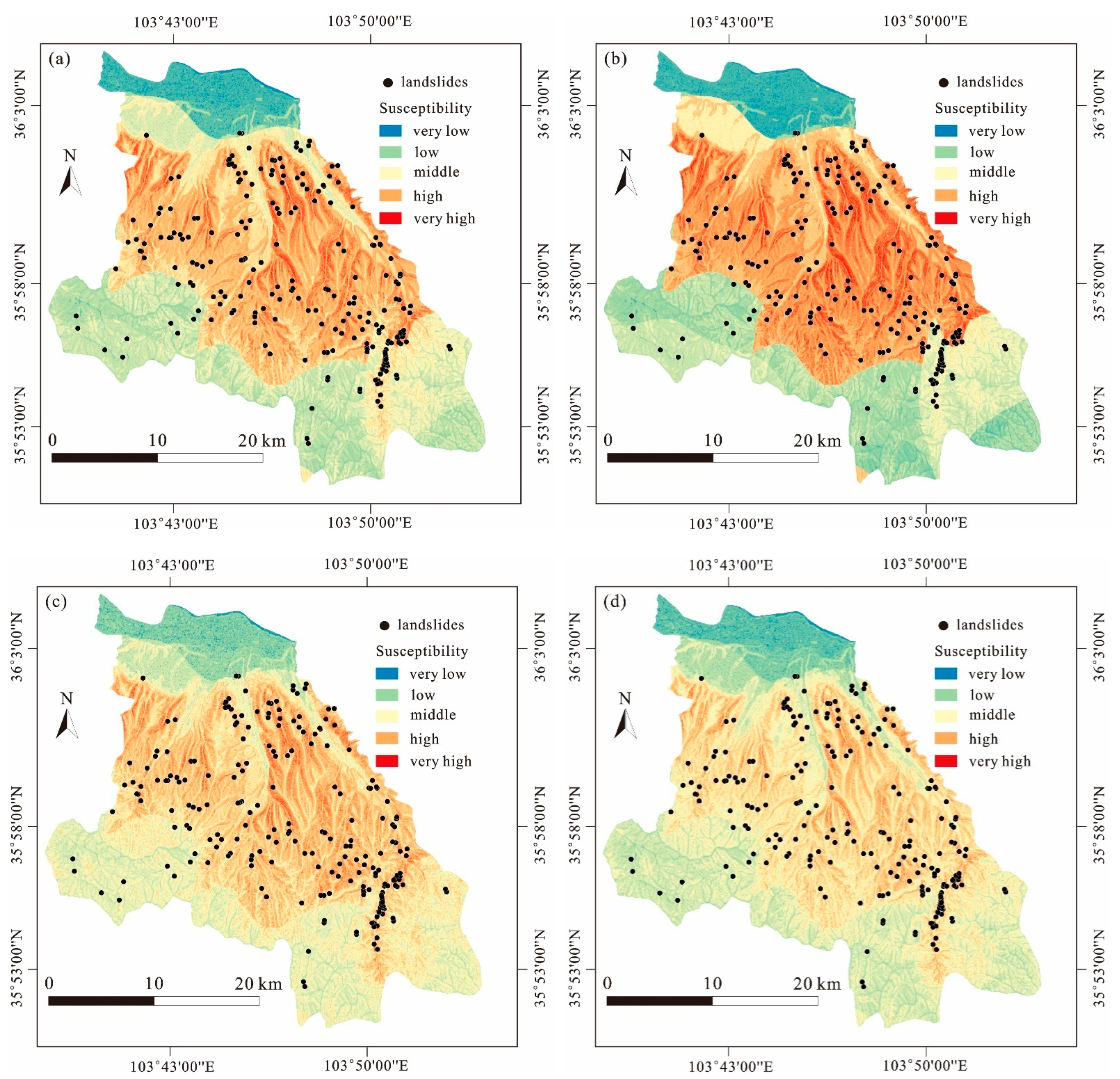
5.2. Landslide Susceptibility Zonation

The landslide susceptibility index at every cell was calculated according to Equation (11) taking into account the two landslide groups separately. The total LSI exhibited similar ranges for different types of landslides: from 0.385 to 1.865 for shallow landslides and from 0.165 to 1.919 for debris flows. The results generated for debris flows had a relatively greater range of LSI, thus indicating a larger contrast between high and low susceptibility zones. This point is confirmed by the landslide susceptibility mapping shown in Figure 9. The zones with very high or high debris flow susceptibilities mostly distributed in the central–eastern part of the study area, most of which were covered by the area with medium elevation and high slope angle. The northern and southwestern parts mostly have very low or low susceptibilities (Figure 9a). This fits with the spatial distribution of debris flows. In fact, the loess area is mainly located in the central part of the study area whereas the southern and northern areas are mostly covered by colluvium, limed soil, and sandy soil. In the area with high slope angles, the collapsibility and high porosity of loess can easily trigger landslides under heavy rainfall conditions, and relative examples have been reported by previous studies [73,74]. The frequency ratio of loess is 1.495 (Table 2), much higher than other categories. Hence, the strong impact of geological factors associated with soil type on the occurrence of this type of landslide is verified. In addition, given that movement characteristics of debris flows, the external topographical factors are also key to controlling the distribution of debris flows; medium elevation and relatively steep slopes provide potential energy for the occurrences, and the channels in such mountainous area provide possible flow paths.

For shallow landslides in the study area, the resulting LSIs are relatively low and the total area of high susceptibility is small (Figure 9b). The zones with very high or high susceptibilities are mainly distributed in the northeastern part of the area, which is the downtown Qilihe District. Another point obviously different from the susceptibility map of debris flow is that the southeastern part of the study area is also high susceptibility. This is mainly because a coal mine is located in this area and the mining activities lasted for decades. Moreover, the national road was also constructed in this area. Hence, these areas are highly populated and with well-developed infrastructure. On one hand, engineering activities (e.g., undercutting of slopes) can result in many steep slopes that may cause precedent deformation of slopes with stress redistribution in soils [75], which are positive for shallow landslides. Furthermore, extensive underground coal mining created much instability (e.g., unstable foundation, surface subsidence, and cracks) and poses a high risk for shallow landslides. Hence, at both sides of the mine, a series of landslides were triggered.

In the last step, the LSIs of two maps were added by using the raster calculator tool in GIS and the landslide susceptibility map for the entire landslide inventory was obtained (Figure 9c). It can be seen that this map combines the characteristics of the two maps above: the zones with very high and high landslide susceptibilities mainly covered the zones near the urban, roads and mining area. The soil type is mostly loess. In the conditions negative for landslides, such as forested area, limed soil, and the area with low slope angles, the susceptibility level evidently decreases. Compared with the landslide points density map (Figure 3a), nearly all of the densely distributed areas of landslides are characterized by very high or high landslide susceptibilities. However, it should be noted that several landslides are located at the zones with very low or low susceptibilities, which are mainly distributed in the southwest part of the study area. Considering that this zone is also recognized as having very low or low susceptibility levels in individual maps (Figure 9a,b), such errors might exist at the beginning and propagated into the final map containing the entire landslide inventory. The northern part is another region with low susceptibility. This is mainly because nearly no historical landslides occurred in this region, so the statistical model identified it as nonprone area for landslides. Furthermore, the elevation in this region is low and slope is flat, which are negative for landsliding.

In conclusion, the susceptibility maps generated for different landslide typologies exhibit differences related to the spatial distribution of susceptibility levels, thus indicating different influences of the same set of input factors. Moreover, the spatial distribution of each type of landslides agrees well with the corresponding higher landslide susceptibility levels.

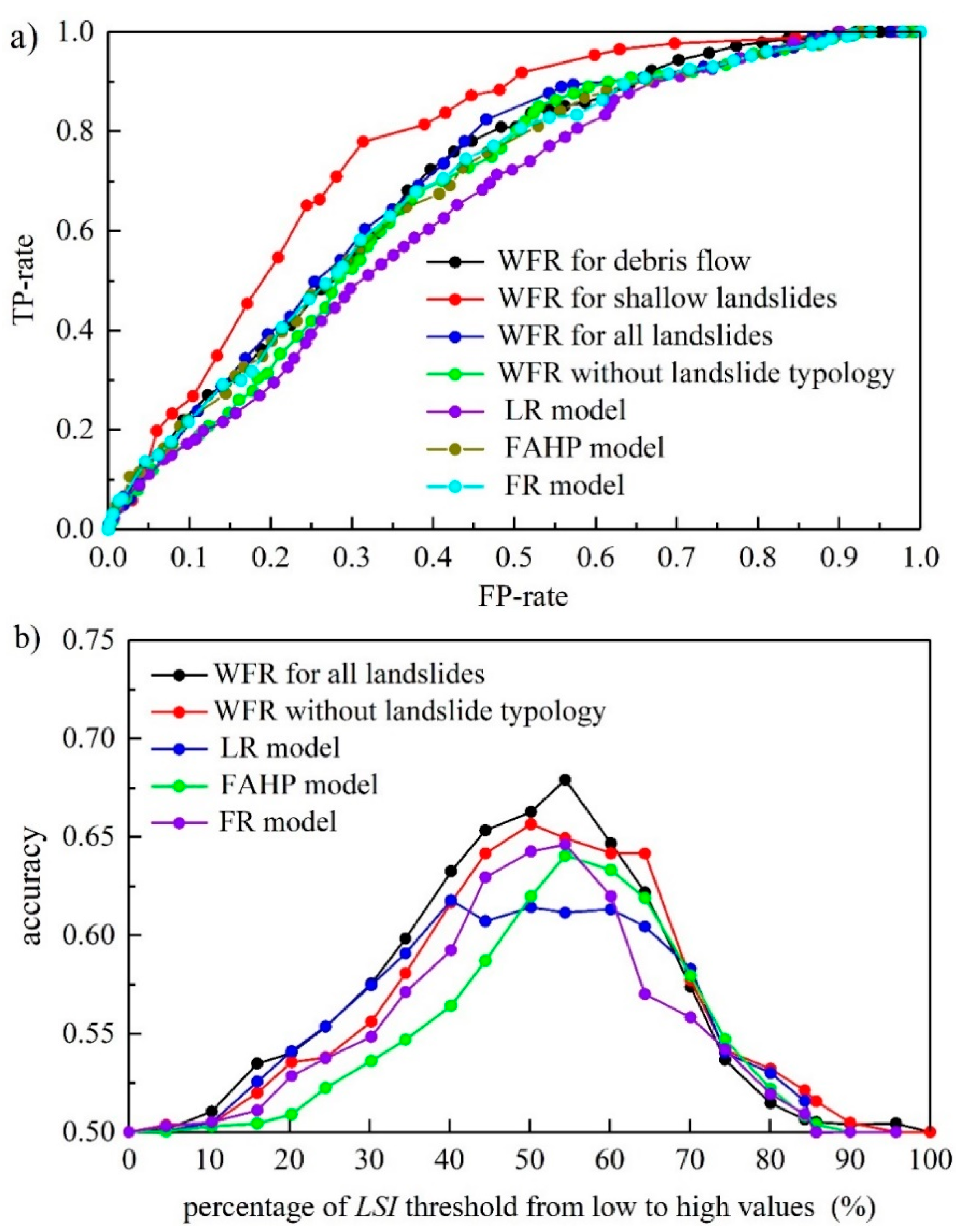
5.3. Model Validation and Comparison

According to Equation (12), Figure 10a presents the values of index R_L in each susceptibility level for the two landslide typologies. Both typologies show evidence and the same tendency: R_L gradually increase when the susceptibility level changed from very low to very high. Especially for the debris flows, the landslide ratio is 0 in the very low susceptibility level while it is more than 6 in the very high susceptibility level. For shallow landslides, all the R_L values in the area with very low, low, and middle are less than 1, while the values in the high and very high susceptibility zones are 3.3 and 4.6, respectively. By combining the LSIs from the two types of landslides, similar results of R_L for the entire landslide inventory in the area are observed: the R_L in high and very high susceptibility zones are 2.1 and 4.5, respectively, which are evidently larger than that of the other susceptibility levels. This difference in R_L shows the concentrated distribution of landslides in the high susceptibility area. The number of landslide pixels in each susceptibility level was counted and the following results obtained: for these three landslide datasets, the proportion of landslides classified into very high or high susceptibility levels are 79.5% (debris flows), 71.3% (shallow landslides), and 73.3% (entire landslide inventory), respectively. It should be noted that the total area with very high and high susceptibilities only cover a small percentage of the whole study area, which are 32.4% (debris flows), 21.2% (shallow landslides), and 32.7% (all of landslides), respectively. As Zêzere [39] concluded, the effectiveness of a model can be validated when the majority of historical unstable slopes concentrate in zones with very high or high susceptibilities. Within the very low and low susceptibility areas, the percentages of landslides are 3.1% (debris flow), 4.7% (shallow landslides), and 3.6% (all of landslides), respectively. This means that the rate of false alerts (landslide inventory points recognized in the low susceptibility area) of the model is low.

Next, 227 landslide points were analyzed in detail by comparing them with 5000 cells randomly selected in the susceptibility maps. The LSIs were divided into 20 intervals on average and the number of landslide and random points in each interval were accounted. The results were normalized in the form of percentage of points versus the LSI for every susceptibility map, which is presented in Figure 10b–d. When the LSIs are low (<50%), the percentage of random points is evidently larger; when the LSIs range from 60~100%, the percentage of landslide points is larger. For these three susceptibility maps, the percentage of landslide points is always the largest between 60% and 70% LSIs. This indicates that most landslides have larger LSIs than random points; thus, the map recognized most landslides. Furthermore, the number of landslides located in the intervals with more than 90% LSIs is relatively small. This is mainly because the area of this susceptibility level is very small.

During the next stage, different models were used to produce landslide susceptibility maps. Although some newly developed models (e.g., some machine learning models) may have better performance [76], the models considered here only included methods relevant to the weighted frequency ratio (WFR) model, because the goal of this part was to verify the rationality of the proposed model, not to find the best model for landslide susceptibility assessment. The models used for comparison were (a) weighted frequency ratio model without taking landslide typology into account, (b) LR model, (c) FAHP model, and (d) FR model. Please note that the last three models also only regarded the entire landslide inventory without including landslide typology. The resulting landslide susceptibility maps are shown in Figure 11. On one side, a detailed receiver operating characteristic (ROC) analysis was adopted to quantitatively clarify their accuracies (Figure 12a). On the other side, the accuracy from the confusion matrix versus LSI thresholds were computed and compared for all these models (Figure 12b). From the perspective of the area under curve (AUC), the WFR model for shallow landslides is the largest (AUC = 0.771) among all the models, thus indicating its better performance. The second largest AUC value is provided by the WFR model using the entire landslide inventory (AUC = 0.704), followed by the WFR model for debris flows (AUC = 0.699), FR model (AUC = 0.689), FAHP model (AUC = 0.686), WFR model without considering landslide typology (AUC = 0.679), and LR model (AUC = 0.650).

From the comparison of LSI threshold with accuracy, the accuracies were similar and relatively stable between the percentages from 40% to 70%. The largest values mostly were in the range of 50~60%. This means the LSI threshold in this range could be used to divide the cells into stable and unstable. Certainly, the selection of an adequate threshold must be a cautious decision, because it is an important index to identify the positive and negative conditions. For this study, the 55% was determined as the LSI threshold because most models had the largest accuracy at this value. Under this situation, the accuracy of the WFR model considering landslide typology was still the best, which was 0.68. The accuracies of other models were 0.66 (WFR model without landslide typology), 0.62 (LR model), 0.65 (FR model), and 0.64 (FAHP model), respectively.

In summary, the present results show that the best performance was given by the WFR model of shallow landslides, while the worst one was the LR model without considering landslide typology. Although the accuracy of the model for the entire landslide inventory considering landslide typology was in the middle level between the accuracies of two landslide typologies, it still was better than all of the other models that did not take landslide typology into account. Hence, if decision-makers want to generate a landslide susceptibility map for the entire landslide dataset of an entire area (not only for a certain landslide typology), the weighted frequency ratio model is a good option.

6. Discussion

In this study, the entire landslide inventory was divided into two types: shallow landslides and debris flows. This is mainly based on geomorphological features and spatial distribution (Section 3.1). In the study area, the shallow landslides occurred in open slopes, whereas debris flows occurred in channels and gullies. Their movement mechanisms are different. This procedure is similar to that reported in previous literature, for example, Zhou et al. [17] divided all landslides in Longju (China) into colluvial landslides and rockfalls; Erener et al. [77] divided landslides in NE Turkey into dormant and active landslides. However, other studies have different attempts on this topic, where researchers classified landslides into different types according to movement pattern or widely accepted criteria [44,45], for example, translational slides and rotational slides. However, it should be noted that in order to incorporate a relatively standard landslide typology into landslide susceptibility assessment, a complete landslide inventory is particularly important. It should allow for recording the relevant information of landslide typology, but unfortunately this is seldom available in many cases, including this study. The dataset in Qilihe was compared with a few studies that performed a standard landslide classification, including Zêzere [39] (144 landslides in an area of 11.3 km²) and Thiery et al. [78] (192 landslides in an area of 100 km²), and it can be found that the preparation of an accurate landslide inventory is often an operational challenge when it comes to regional scale studies, particularly for our study (227 landslides in an area of 395 km²). However, as Corominas et al. [36] summarized, it is difficult to provide strict guidelines for the type of data required in a landslide risk analysis. Hence, in this study, the landslide typology was determined mainly according to triggering factors and geomorphological features. On one hand, the lack of detailed information on standard landslide typology makes the traditional classification impossible; on other hand, the analysis on landslide point density does indicate an evident difference between the two landslide types. Hence, in spite of historical data that may be lacking, the present classification is acceptable for a preliminary analysis.

The proposed weighted frequency ratio model to assess the regional-scale landslide susceptibility is fundamentally a statistically based method because it can quantitatively present the contribution of influencing factors or their categories in the modeling procedure. Our work indicates that soil and land use are relatively important for debris flows whereas slope is of small importance; for shallow landslides, soil and relief degree of land surface are the most important among the prediction factors. Some of these findings contradict those of previous studies. For instance, Hürlimann et al. [79] found that slope angle between 30° and 35° is the most significant factor for the rainfall-induced flows in the Pyrenees. Wu et al. [54] tested the importance of input factors using machine learning methods in an area with a setting similar to this study, and recorded a moderate contribution of geological factors. This leads us to conclude that the model performance depends much on input datasets (e.g., quality, availability, and type) and the types of model used, so it may vary with different cases. Given the difference among the development laws of each landslide typology at a regional scale, it is not easy to directly extrapolate an empirical landslide susceptibility model to neighboring regions. Moreover, another limitation of this study related to the selection of influencing factors; each landslide type should have specific conditioning factors that depend on the mechanism. It is therefore important to adopt different sets of influencing factors to assess landslide susceptibility. This means different numbers and types of factors are required to distinguish the occurrence conditions for different landslide types. However, in our study, only the weight of every factor was changed without considering different combinations of the factors. As some classic literature (e.g., [44]) have already stated, the fact that different types of landslides occur in different conditions is evident. Hence, subsequent analysis should deal with these conditions in different landslides types.

To obtain a reliable result, a set of easy-to-obtain geological or environmental data were used to produce thematic maps as input variables. Although several of them are still debated (e.g., RDLS and SCA) and are not commonly mentioned in previous literature, the twelve influencing factors used in this study fit well with the assertion that landslides are controlled by mechanical laws that can be determined empirically, statistically, or in an indeterministic fashion [5]. In fact, the linear statistical relationship on landslide number and factors indicates they do affect landslide occurrences. For debris flows, there is an evident positive correlation between frequency ratio and RDLS, and the FR value in the category of 120~140 is larger than most categories (including other factors). For shallow landslides, the weight of SCA is higher than some commonly used factors, such as curvature and land use. Certainly, this does not mean that more new influencing factors could be taken into account of the modeling casually; on the contrary, our study indicates that the selection of influencing factors should not only use other methods described in the literature for reference, but also take the geological/environmental settings of the test site into account. Hence, as Segoni et al. [80] suggested, researchers should have a good understanding of the geological meaning of the units defined in their maps because the difference among geological units may have a deep influence on the effectiveness of susceptibility modeling. This process can be conducted by using a variety of methods, such as field survey on the test site, review of existing literature, and examination of historical data, among others. In the present study, these geological meanings were recognized mainly through field work and archived documents (e.g., landslide triggers and historical engineering activities). During the next stage, a statistical tool in GIS (density analysis of landslide points) was adopted to perform back analysis to validate their significance on landslide occurrence.

In terms of model performance, the accuracy of the proposed model is only approximately 70%, which is much closer to other studies using the same type of approach (e.g., the mean AUC of 0.74 in [81]; the maximum AUC of 0.71 in [82]; the AUC of 0.75 in [83]). It must be admitted that this accuracy is not superior, which mainly includes two reasons: one is that the data quality of the inventory is not very high, and the other is associated with the limitation of statistically based methods. The main limitation on landslide inventory is that we used landslide initiation points and not polygons as sampling data. Point data of landslide occurrence ignore the size, volume, and magnitude; as a result, landslide susceptibility mapping can be biased. Hence, our next work should consider landslide polygons to prepare landslide susceptibility mapping. Related work can be seen in Catani et al. [37]. Users should be careful, however, on this point because polygon data also have the drawback of being subjective; independent researchers may produce very different landslide susceptibility mappings in the same study area, which can result in spatial positioning inconsistencies in the boundaries of mapped landslide polygons [84]. Considering this point, landslide point data are still used in some studies worldwide [20,25].

Although the present model did not increase the accuracy by much, it does offer an improvement compared with the basic version of the model. In other words, we think the current result is acceptable for a preliminary analysis because what we concern the most is to discuss the rationality of landslide classification by using the weighted frequency ratio model, which can be considered in landslide susceptibility assessment, rather than the comparison of methodologies. This mainly addresses an operational and technical challenge: when it comes to a landslide inventory that includes more than one landslide type, landslide susceptibility mapping for the entire landslide dataset is still possible and the modeling process allows for reflecting the different incidences of a same group of input factors. It is a main topical issue currently in this research niche [85]. Moreover, it has a more complete geomorphological meaning; traditionally data-driven approaches (including statistically based approaches and machine learning approaches) mostly only analyze the nonlinear relationship between landslide and input factors without concentrating on geomorphological implications involved in the landslide process. These models usually can perform accurate prediction on landslide spatial distribution, but fail to explain the obtained results from a geomorphological point of view. However, geomorphology attributes are quite important in the Loess Plateau of China because it has been confirmed that landslide types have a close relationship with it [86]. Regarding the model accuracy, in fact, along with the development of GIS and machine learning techniques, a trend toward advanced but complicated landslide susceptibility models has shown up. Hence, it can be believed that a better model will be found in future work that not only allows consideration of the landslide typology, but also has a satisfactory model performance.

7. Conclusions

This study aims at incorporating landslide typology into landslide susceptibility assessment of Qilihe District in Lanzhou (northwestern China), and individually establishing an influencing factor system for each type of landslide to create an effective landslide susceptibility map. For this purpose, a WFR model was proposed, where the LR–FAHP approach was used to calculate the weight of influencing factors, and the rank among different categories within each factor was determined by the FR method. According to the analysis of landslide spatial distribution and geomorphological features, all of the landslides in the region were classified into two categories: debris flows and shallow landslides. Based on 12 thematic layers, the WFR model was demonstrated to be effective when mapping the landslide susceptibility; the accuracy presented by AUC was 70.4%. Such accuracy was better than that of the individual LR, FAHP, and FR models. When all landslides were considered as a group from the beginning, the accuracy of landslide susceptibility assessment was reduced by 1.5~5.4%.

Summarizing, the current results reveal that more reliable landslide susceptibility maps can be produced when landslide typology is incorporated into the modeling process. Therefore, it is highly recommended to separately conduct susceptibility assessment for each type of landslide instead of as a whole group. However, it should be noted that the eventual map was determined by combining individual susceptibility maps for each landslide type. This means the error in every individual map may be propagated into the final results. In this study, the resulting accuracy of shallow landslides is nearly 80% while that of debris flows is only approximately 70%. These results suggest that more work is needed before applying the proposed procedure to other cases. There are two potential tasks in our future work: one is to improve the accuracy of individual landslide susceptibility maps by comparing methodologies; the other is to simplify or optimize the influencing factor combination, especially under the condition that the weight of factors can be obtained by the existing model.

References

1. Aristizábal, E.; Vélez, J.I.; Martínez, H.E.; Jaboyedoff, M. SHIA_Landslide: A distributed conceptual and physically based model to forecast the temporal and spatial occurrence of shallow landslides triggered by rainfall in tropical and mountainous basins. Landslides 2016, 13, 497–517. [Google Scholar] [CrossRef]
2. Froude, M.J.; Petley, D.N. Global fatal landslide occurrence from 2004–2016. Nat. Hazards Earth Syst. Sci. 2018, 18, 2161–2181. [Google Scholar] [CrossRef]
3. Kappes, M.S.; Keiler, M.; von Elverfeldt, K.; Glade, T. Challenges of analyzing multi-hazard risk: A review. Nat. Hazards 2012, 64, 1925–1958. [Google Scholar] [CrossRef]
4. Guo, Z.; Chen, L.; Yin, K.; Shrestha, D.P.; Zhang, L. Quantitative risk assessment of slow-moving landslides from the viewpoint of decision-making: A case study of the Three Gorges Reservoir in China. Eng. Geol. 2020, 273, 105667. [Google Scholar] [CrossRef]
5. Guzzetti, F.; Carrara, A.; Cardinali, M.; Reichenbach, P. Landslide hazard evaluation: A review of current techniques and their application in a multi-scale study, Central Italy. Geomorphology 1999, 31, 181–216. [Google Scholar] [CrossRef]
6. Guzzetti, F.; Reichenbach, P.; Ardizzone, F.; Cardinali, M.; Galli, M. Estimating the quality of landslide susceptibility models. Geomorphology 2006, 81, 166–184. [Google Scholar] [CrossRef]
7. Dai, F.C.; Lee, C.F. Landslide characteristics and slope instability modeling using GIS Lantau Island, Hong Kong. Geomorphology 2002, 42, 213–238. [Google Scholar] [CrossRef]
8. Huang, F.; Yin, K.; Huang, J.; Gui, L.; Wang, P. Landslide susceptibility mapping based on self-organizing-map network and extreme learning machine. Eng. Geol. 2017, 223, 11–22. [Google Scholar] [CrossRef]
9. Bueechi, E.; Klimeš, J.; Frey, H.; Huggel, C.; Strozzi, T.; Cochachin, A. Regional-scale landslide susceptibility modelling in the Cordillera Blanca, Peru—a comparison of different approaches. Landslides 2019, 16, 395–407. [Google Scholar] [CrossRef]
10. Guo, Z.; Yin, K.; Fu, S.; Huang, F.; Gui, L.; Xia, H. Evaluation of landslide susceptibility based on GIS and WOE-BP model. Earth Sci. 2019, 44, 4299–4312. [Google Scholar]
11. Zêzere, J.; Pereira, S.; Melo, R.; Oliveira, S.; Garcia, R. Mapping landslide susceptibility using data-driven methods. Sci. Total Environ. 2017, 589, 250–267. [Google Scholar] [CrossRef] [PubMed]
12. Reichenbach, P.; Rossi, M.; Malamud, B.D.; Mihir, M.; Guzzetti, F. A review of statistically-based landslide susceptibility models. Earth Sci. Rev. 2018, 180, 60–91. [Google Scholar] [CrossRef]
13. Goetz, J.N.; Brenning, A.; Petschko, H.; Leopold, P. Evaluating machine learning and statistical prediction techniques for landslide susceptibility modeling. Comput. Geosci. 2015, 81, 1–11. [Google Scholar] [CrossRef]
14. Xiao, T.; Segoni, S.; Chen, L.; Yin, K.; Casagli, N. A step beyond landslide susceptibility maps: A simple method to investigate and explain the different out-comes obtained by different approaches. Landslides 2020, 17, 627–640. [Google Scholar] [CrossRef]
15. Yilmaz, I. Landslide susceptibility mapping using frequency ratio, logistic regression, artificial neural networks and their comparison: A case study from Kat landslides (Tokat-Turkey). Comput. Geosci. 2009, 35, 1125–1138. [Google Scholar] [CrossRef]
16. Marjanović, M.; Kovačević, M.; Bajat, B.; Voženílek, V. Landslide susceptibility assessment using SVM machine learning algorithm. Eng. Geol. 2011, 123, 225–234. [Google Scholar] [CrossRef]
17. Zhou, C.; Yin, K.; Cao, Y.; Ahmed, B.; Li, Y.; Catani, F.; Pourghasemi, H.R. Landslide susceptibility modeling applying machine learning methods: A case study from Longju in the Three Gorges Reservoir area, China. Comput. Geosci. 2018, 112, 23–37. [Google Scholar] [CrossRef]
18. Yeon, Y.-K.; Han, J.-G.; Ryu, K.H. Landslide susceptibility mapping in Injae, Korea, using a decision tree. Eng. Geol. 2010, 116, 274–283. [Google Scholar] [CrossRef]
19. Arabameri, A.; Chen, W.; Loche, M.; Zhao, X.; Li, Y.; Lombardo, L.; Cerda, A.; Pradhan, B.; Bui, D.T. Comparison of machine learning models for gully erosion susceptibility mapping. Geosci. Front. 2020, 11, 1609–1620. [Google Scholar] [CrossRef]
20. Huang, F.; Cao, Z.; Guo, J.; Jiang, S.-H.; Li, S.; Guo, Z. Comparisons of heuristic, general statistical and machine learning models for landslide susceptibility prediction and mapping. Catena 2020, 191, 104580. [Google Scholar] [CrossRef]
21. Ayalew, L.; Yamagishi, H. The application of GIS-based logistic regression for landslide susceptibility mapping in the Kakuda-Yahiko mountains Central Ja-pan. Geomorphology 2005, 65, 15–31. [Google Scholar] [CrossRef]
22. Mousavi, S.Z.; Kavian, A.; Soleimani, K.; Mousavi, S.R.; Shirzadi, A. GIS-based spatial prediction of landslide susceptibility using logistic regression model. Geomat. Nat. Hazards Risk. 2011, 2, 33–50. [Google Scholar] [CrossRef]
23. Raja, N.B.; Cicek, I.; Türkoglu, N.; Aydin, O.; Kawasaki, A. Landslide susceptibility mapping of the Sera River Basin using logistic regression model. Nat. Hazards 2017, 85, 1323–1346. [Google Scholar] [CrossRef]
24. Brenning, A. Benchmarking classifiers to optimally integrate terrain analysis and multispectral remote sensing in automatic rock glacier detection. Remote Sens. Environ. 2009, 113, 239–247. [Google Scholar] [CrossRef]
25. Goetz, J.N.; Guthrie, R.H.; Brenning, A. Integrating physical and empirical landslide susceptibility models using generalized additive models. Geomorphology 2011, 129, 376–386. [Google Scholar] [CrossRef]
26. Cao, J.; Zhang, Z.; Wang, C.; Liu, J.; Zhang, L. Susceptibility assessment of landslides triggered by earthquakes in the Western Sichuan Plateau. Catena 2019, 175, 63–76. [Google Scholar] [CrossRef]
27. Roodposhti, M.S.; Rahimi, S.; Beglou, M.J. PROMETHEE II and fuzzy AHP: An enhanced GIS-based landslide susceptibility mapping. Nat. Hazards 2014, 73, 77–95. [Google Scholar] [CrossRef]
28. Mallick, J.; Singh, R.K.; AlAwadh, M.A.; Islam, S.; Khan, R.A.; Qureshi, M.N. GIS-based landslide susceptibility evaluation using fuzzy-AHP multi-criteria decision-making techniques in the Abha Watershed, Saudi Arabia. Environ. Earth Sci. 2018, 77, 276–300. [Google Scholar] [CrossRef]
29. Yalcin, A.; Reis, S.; Aydinoglu, A.C.; Yomralioglu, T. A GIS-based comparative study of frequency ratio, analytical hierarchy process, bivariate statistics and logistics regression methods for landslide susceptibility mapping in Trabzon, NE Turkey. Catena 2011, 85, 274–287. [Google Scholar] [CrossRef]
30. Batar, A.K.; Watanabe, T. Landslide susceptibility mapping and assessment using geospatial platforms and weights of evidence (WoE) method in the Indian Himalayan region: Recent developments, gaps, and future directions. ISPRS Int. J. Geoinf. 2021, 10, 114. [Google Scholar] [CrossRef]
31. Xu, W.; Yu, W.; Jing, S.; Zhang, G.; Huang, J. Debris flow susceptibility assessment by GIS and information value model in a large-scale region, Sichuan Province (China). Nat. Hazards 2013, 65, 1379–1392. [Google Scholar] [CrossRef]
32. Shirani, K.; Pasandi, M.; Arabameri, A. Landslide susceptibility assessment by Dempster–Shafer and index of entropy models, Sarkhoun basin, Southwestern Iran. Nat. Hazards 2018, 93, 1379–1418. [Google Scholar] [CrossRef]
33. Yilmaz, I. Comparison of landslide susceptibility mapping methodologies for Koyulhisar, Turkey: Conditional probability, logistic regression, artificial neural networks, and support vector machine. Environ. Earth Sci. 2010, 61, 821–836. [Google Scholar] [CrossRef]
34. Fan, W.; Wei, X.S.; Cao, Y.B.; Zheng, B. Landslide susceptibility assessment using the certainty factor and analytic hierarchy process. J. Mt. Sci. 2017, 14, 906–925. [Google Scholar] [CrossRef]
35. Park, N.-W. Application of Dempster-Shafer theory of evidence to GIS-based landslide susceptibility analysis. Environ. Earth Sci. 2011, 62, 367–376. [Google Scholar] [CrossRef]
36. Corominas, J.; Van Westen, C.; Frattini, P.; Cascini, L.; Malet, J.-P.; Fotopoulou, S.; Catani, F.; Eeckhaut, M.V.D.; Mavrouli, O.; Agliardi, F.; et al. Recommendations for the quantitative analysis of landslide risk. Bull. Int. Assoc. Eng. Geol. 2013, 73, 209–263. [Google Scholar] [CrossRef]
37. Catani, F.; Lagomarsino, D.; Segoni, S.; Tofani, V. Landslide susceptibility estimation by random forests technique: Sensitivity and scaling issues. Nat. Hazards Earth Syst. Sci. 2013, 13, 2815–2831. [Google Scholar] [CrossRef]
38. Lee, S.; Ryu, J.-H.; Won, J.-S.; Park, H.-J. Determination and application of the weights for landslide susceptibility mapping using an artificial neural network. Eng. Geol. 2004, 71, 289–302. [Google Scholar] [CrossRef]
39. Zêzere, J.L. Landslide susceptibility assessment considering landslide typology: A case study in the area north of Lisbon (Portugal). Nat. Hazards Earth Syst. Sci. 2002, 2, 73–82. [Google Scholar] [CrossRef]
40. Epifânio, B.; Zêzere, J.L.; Neves, M. Susceptibility assessment to different types of landslides in the coastal cliffs of Lourinhã (Central Portugal). J. Sea Res. 2014, 93, 150–159. [Google Scholar] [CrossRef]
41. Shu, H. Study on the Formation and Motion Characteristics of Debris Flow in Small Watershed in Hilly Region of Loess Area. Ph.D. Thesis, Lanzhou University, Lanzhou, China, 2019. (In Chinese). [Google Scholar]
42. Meng, C.; Yang, Y.; Hu, H. A GIS-based urban landscape study of Lanzhou City, China. In Proceedings of the 19th International Conference on Geoinformatics, Shanghai, China, 24–26 June 2011; pp. 1–5. [Google Scholar]
43. Tian, Y.; Xu, C.; Ma, S.; Wang, S.; Zhang, H. Inventory and spatial distribution of landslides triggered by the 8th August 2017 MW 6.5 Jiuzhaigou earthquake, China. J. Earth Sci. 2019, 30, 206–217. [Google Scholar]
44. Cruden, D.M.; Varnes, D.J. Landslide types and processes. In Landslides Investigation and Mit-igation; Turner, A.K., Schuster, R.L., Eds.; Transportation Research Board; Special Report 247; US National Research Council: Washington, DC, USA, 1996; pp. 36–75. [Google Scholar]
45. Hungr, O.; Leroueil, S.; Picarelli, L. The Varnes classification of landslide types, an update. Landslides 2014, 11, 167–194. [Google Scholar] [CrossRef]
46. Hürlimann, M.; Coviello, V.; Bel, C.; Guo, X.; Berti, M.; Graf, C.; Hübl, J.; Miyata, S.; Smith, J.B.; Yin, H.Y. Debris-flow monitoring and warning: Review and examples. Earth Sci. Rev. 2019, 199, 102981. [Google Scholar] [CrossRef]
47. Criss, R.E.; Yao, W.; Li, C.; Tang, H. A predictive, two-parameter model for the movement of reservoir landslides. J. Earth. Sci. 2020, 31, 1051–1057. [Google Scholar] [CrossRef]
48. Kayastha, P.; Dhital, M.R.; Smedt, F.D. Application of the analytical hierarchy process (AHP) for landslide susceptibility mapping: A case study from the Tinau watershed, west Nepal. Comput. Geosci. 2013, 52, 398–408. [Google Scholar] [CrossRef]
49. Zhang, G.; Cai, Y.; Zheng, Z.; Zhen, J.; Liu, Y.; Huang, K. Integration of the statistical index method and the analytic hierarchy process technique for the assessment of landslide susceptibility in Huizhou, China. Catena 2016, 142, 233–244. [Google Scholar] [CrossRef]
50. Chen, V.Y.C.; Lien, H.P.; Liu, C.H.; Liou, J.J.H.; Tzeng, G.H.; Yang, L.S. Fuzzy MCDM approach for selecting the best environment-watershed plan. Appl. Soft Comput. 2011, 11, 265–275. [Google Scholar] [CrossRef]
51. Feizizadeh, B.; Roodposhti, M.S.; Jankowski, P.; Blaschke, T. A GIS-based extended fuzzy multi-criteria evaluation for landslide susceptibility mapping. Comput. Geosci. 2014, 73, 208–221. [Google Scholar] [CrossRef]
52. Catani, F.; Casagli, N.; Ermini, L.; Righini, G.; Menduni, G. Landslide hazard and risk mapping at catchment scale in the Arno River Basin. Landslides 2005, 2, 329–343. [Google Scholar] [CrossRef]
53. Aditian, A.; Kubota, T.; Shinohara, Y. Comparison of GIS-based landslide susceptibility models using frequency ratio, logistic regression, and artificial neural network in a tertiary region of Ambon, Indonesia. Geomorphology 2018, 318, 101–111. [Google Scholar] [CrossRef]
54. Wu, Y.; Ke, Y.; Chen, Z.; Liang, S.; Zhao, H.; Hong, H. Application of alternating decision tree with AdaBoost and bagging ensembles for landslide susceptibility mapping. Catena 2020, 187, 104396. [Google Scholar] [CrossRef]
55. Pereira, S.; Zêzere, J.L.; Bateira, C. Technical Note: Assessing predictive capacity and conditional independence of landslide predisposing factors for shallow landslide susceptibility models. Nat. Hazards Earth Syst. Sci. 2012, 12, 979–988. [Google Scholar] [CrossRef]
56. Tang, Y.; Feng, F.; Guo, Z.; Feng, W.; Li, Z.; Wang, J.; Sun, Q.; Ma, H.; Li, Y. Integrating principal component analysis with statistically-based models for analysis of causal factors and landslide susceptibility mapping: A comparative study from the loess plateau area in Shanxi (China). J. Clean. Prod. 2020, 277, 124159. [Google Scholar]
57. Cama, M.; Nicu, I.C.; Conoscenti, C.; Quénéhervé, G.; Maerker, M. The Role of Multicollinearity in Landslide Susceptibility Assessment by Means of Binary Logistic Regression: Comparison Between VIF and AIC Stepwise Selection; EGU General Assembly Conference Abstract: Vienna, Austria, 2016. [Google Scholar]
58. Kouli, M.; Loupasakis, C.; Soupios, P.; Rozos, D.; Vallianatos, F. Landslide susceptibility mapping by comparing the WLC and WofE multi-criteria methods in the West Crete Island, Greece. Environ. Earth Sci. 2014, 72, 5197–5219. [Google Scholar] [CrossRef]
59. Peng, L.; Niu, R.; Huang, B.; Wu, X.; Zhao, Y.; Ye, R. Landslide susceptibility mapping based on rough set theory and support vector machines: A case of the Three Gorges area, China. Geomorphology 2014, 204, 287–301. [Google Scholar] [CrossRef]
60. Correa-Muñoz, N.A.; Murilli-Feo, C.A.; Martínez-Martíne, L.J. The potential of PALSAR RTC elevation data for landform semi-automatic detection and landslide susceptibility modeling. Eur. J. Remote Sens. 2019, 52, 149–159. [Google Scholar] [CrossRef]
61. Liu, J.; Duan, Z. Quantitative assessment of landslide susceptibility comparing statistical index, index of entropy, and weights of evidence in the shangnan area, China. Entropy 2018, 20, 868. [Google Scholar] [CrossRef] [PubMed]
62. Chang, K.-T.; Merghadi, A.; Yunus, A.P.; Pham, B.T.; Dou, J. Evaluating scale effects of topographic variables in landslide susceptibility models using GIS-based machine learning techniques. Sci. Rep. 2019, 9, 1–21. [Google Scholar] [CrossRef] [PubMed]
63. Nefeslioglu, H.A.; Duman, T.Y.; Durmaz, S. Landslide susceptibility mapping for a part of tectonic Kelkit Valley (Eastern Black Sea region of Turkey). Geomorphology 2008, 94, 401–418. [Google Scholar] [CrossRef]
64. Wang, Q.; Li, W.; Chen, W.; Bai, H. GIS-based assessment of landslide susceptibility using certainty factor and index of entropy models for the Qianyang County of Baoji city, China. J. Earth Syst. Sci. 2015, 124, 1399–1415. [Google Scholar] [CrossRef]
65. Huang, F.; Yao, C.; Liu, W.; Li, Y.; Liu, X. Landslide susceptibility assessment in the Nantian area of China: A comparison of frequency ratio model and support vector machine. Geomat. Nat. Hazards Risk. 2018, 9, 919–938. [Google Scholar] [CrossRef]
66. Guisan, A.; Weiss, S.B.; Weiss, A.D. GLM versus CCA spatial modeling of plant species distribution. Plant Ecol. 1999, 143, 107–122. [Google Scholar] [CrossRef]
67. Weiss, A. Topographic Position and Landforms Analysis; Poster presentation; ESRI User Conference: San Diego, CA, USA, 2001. [Google Scholar]
68. Shu, H.; Hürlimann, M.; Molowny-Horas, R.; González, M.; Pinyol, J.; Abancó, C.; Ma, J. Relation between land cover and landslide susceptibility in Val d’Aran, Pyrenees (Spain): Historical aspects, present situation and forward prediction. Sci. Total Environ. 2019, 693, 133557. [Google Scholar] [CrossRef] [PubMed]
69. Sørensen, R.; Zinko, U.; Seibert, J. On the calculation of the topographic wetness index: Evaluation of different methods based on field observations. Hydro. Earth Syst. Sci. 2006, 10, 101–112. [Google Scholar] [CrossRef]
70. Moore, I.D.; Grayson, R.B.; Ladson, A.R. Digital terrain modeling: A review of hydrological, geomorphological, and biological applications. Hydrol. Process. 1991, 5, 3–30. [Google Scholar] [CrossRef]
71. Coelho-Netto, A.L.; Avelar, A.S.; Fernandes, M.C.; Lacerda, W.A. Landslide susceptibility in a mountainous geoecosystem, Tijuca Massif, Rio de Janeiro: The role of morphometric subdivision of the terrain. Geomorphology 2007, 87, 120–131. [Google Scholar] [CrossRef]
72. Zhang, Y.; Chen, N.; Liu, M.; Wang, T.; Deng, M.; Wu, K.; Khanal, B.R. Debris flows originating from colluvium deposits in hollow regions during a heavy storm process in Taining, southeastern China. Landslides 2020, 17, 335–347. [Google Scholar] [CrossRef]
73. Shu, H.; Ma, J.; Qi, S.; Chen, P.; Guo, Z.; Zhang, P. Experimental results of the impact pressure of debris flows in loess regions. Nat. Hazards 2020, 103, 3329–3356. [Google Scholar] [CrossRef]
74. Shu, H.; Ma, J.; Guo, J.; Qi, S.; Guo, Z.; Zhang, P. Effects of rainfall on surface environment and morphological characteristics in the Loess Plateau. Environ. Sci. Pollut. Res. 2020, 27, 37455–37467. [Google Scholar] [CrossRef]
75. Deng, Q.; Fu, M.; Ren, X.; Liu, F.; Tang, H. Precedent long-term gravitational deformation of large scale landslides in the Three Gorges reservoir area, China. Eng. Geol. 2017, 221, 170–183. [Google Scholar] [CrossRef]
76. Achour, Y.; Pourghasemi, H.R. How do machine learning techniques help in increasing accuracy of landslides susceptibility maps? Geosci. Front. 2020, 11, 871–883. [Google Scholar] [CrossRef]
77. Erener, A.; Mutlu, A.; Düzgün, H.S. A comparative study for landslide susceptibility mapping using GIS-based multi-criteria decision analysis (MCDA), logistic regression (LR) and association rule mining (ARM). Eng. Geol. 2016, 203, 45–55. [Google Scholar] [CrossRef]
78. Thiery, Y.; Malet, J.-P.; Sterlacchini, S.; Puissant, A.; Maquaire, O. Landslide susceptibility assessment by bivariate methods at large scales: Application to a complex mountainous environment. Geomorphology 2007, 92, 38–59. [Google Scholar] [CrossRef]
79. Hürlimann, M.; Lantada, N.; González, M.; Pinyol, J. Susceptibility assessment of rainfall-triggered flows and slides in the central-eastern Pyrenees. In Landslides and Engineered Slopes. Experience, Theory and Practice, Proceedings of the 12th International Symposium on Landslides, Napoli, Rome, 12–19 June 2016; CRC Press: Boca Raton, FL, USA, 2016; pp. 1129–1136. [Google Scholar]
80. Segoni, S.; Pappafico, G.; Luti, T.; Catani, F. Landslide susceptibility assessment in complex geological settings: Sensitivity to geological information and insights on its parameterization. Landslides 2020, 17, 2443–2453. [Google Scholar] [CrossRef]
81. Conoscenti, C.; Rotigliano, E.; Cama, M.; Caraballo-Arias, N.A.; Lombardo, L.; Agnesi, V. Exploring the effect of absence selection on landslide susceptibility models: A case study in Sicily, Italy. Geomorphology 2016, 261, 222–235. [Google Scholar] [CrossRef]
82. Camilo, D.C.; Lombardo, L.; Mai, P.M.; Dou, J.; Huser, R. Handling high predictor dimensionality in slope-unit-based landslide susceptibility models through LASSO-penalized Generalized Linear Model. Environ. Model. Softw. 2017, 97, 145–156. [Google Scholar] [CrossRef]
83. Youssef, A.M.; Al-Kathery, M.; Pradhan, B. Landslide susceptibility mapping at Al-Hasher area, Jizan (Saudi Arabia) using GIS-based frequency ratio and index of entropy models. Geosci. J. 2015, 19, 113–134. [Google Scholar] [CrossRef]
84. Ardizzone, F.; Cardinali, M.; Carrara, A.; Guzzetti, F.; Reichenbach, P. Impact of mapping errors on the reliability of landslide hazard maps. Nat. Hazards Earth Syst. Sci. 2002, 2, 3–14. [Google Scholar] [CrossRef]
85. Orimoloye, I.; Ekundayo, T.C.; Ololade, O.O.; Belle, J.A. Systematic mapping of disaster risk management research and the role of innovative technology. Environ. Sci. Pollut. Res. 2021, 28, 4289–4306. [Google Scholar] [CrossRef]
86. Zhang, F.; Chen, W.; Liu, G.; Liang, S.; Kang, C.; He, F. Relationships between landslide types and topographic attributes in a loess catchment, China. J. Mt. Sci. 2012, 9, 742–751. [Google Scholar] [CrossRef]
Figure 1. (a) Location of Lanzhou City and its 2020 remote sensing image from Google Earth, and (b) the topography map showing the elevation of Qilihe District.
Remotesensing 13 03623 g001
Figure 2. Several typical landslides in the inventory: (a) a shallow earth slide in a translational form triggered by the road construction, (b) a small-scale landslide composed of loess and triggered by rainfall, (c) a debris flow in a channel, and (d) an earth flow composed of loess.
Remotesensing 13 03623 g002aRemotesensing 13 03623 g002b
Figure 3. (a) Density of landslide points and locations of geological faults, roads, and the mining area in the study area. (b) Cross-section A–A’ showing elevations extracted by the GIS tool.
Remotesensing 13 03623 g003aRemotesensing 13 03623 g003b
Figure 4. Remote sensing images from Google Earth in 2020 showing the geomorphology of the study area: (a) Huangyu gulley, (b) Agan town and nearby mining area, and (c) the urban area in the northern part of Qilihe District where buildings and roads are highly concentrated.
Remotesensing 13 03623 g004
Figure 5. Typical schematic models for the landslides: (a) debris flows induced by rainfall which affect human settlements (modified according to https://geology.com/articles/debris-flow/ accessed on 5 January 2021), (b) shallow landslides composed of loess triggered by rainfall and undercutting of slopes (modified according to https://www.geotech.hr/en/landslides/ accessed on 5 January 2021).
Remotesensing 13 03623 g005
Figure 6. The spatial distribution of two types of landslides in Qilihe District using the digital elevation model (DEM) as the base map.
Remotesensing 13 03623 g006
Figure 7. Thematic maps of influencing factors: (a) elevation, (b) slope, (c) aspect, (d) curvature, (e) RDLS, (f) TPI, (g) soil, (h) lithology, (i) land use, (j) SPI, (k) TWI, (l) SCA.
Remotesensing 13 03623 g007aRemotesensing 13 03623 g007b
Figure 8. Workflow of this study.
Remotesensing 13 03623 g008
Figure 9. Landslide susceptibility mapping using the weighted frequency ratio model: (a) for shallow landslides, (b) for debris flows, and (c) for all landslides in the study area.
Remotesensing 13 03623 g009
Figure 10. Evaluation of the LR–FAHP model considering landslide typology: (a) values of RL in each landslide susceptibility level for both landslide typologies; comparisons of LSI distribution between landslide points and random points: (b) debris flows, (c) shallow landslides, and (d) all landslides.
Remotesensing 13 03623 g010
Figure 11. Landslide susceptibility maps obtained from different models: (a) weighted frequency ratio model without considering landslide typology, (b) logistic regression model, (c) fuzzy analytical hierarchy process model, and (d) frequency ratio model.
Remotesensing 13 03623 g011
Figure 12. Accuracy analysis and comparison of susceptibility maps for the Qilihe District using different models: (a) results of receiver operating characteristic curves and (b) threshold of LSI versus accuracy curves.
Remotesensing 13 03623 g012