
Approaching Global Instantaneous Precise Positioning with the Dual- and Triple-Frequency Multi-GNSS Decoupled Clock Model


Department of Earth and Space Science and Engineering, York University, Toronto, ON M3J 1P3, Canada
*
Author to whom correspondence should be addressed.
Remote Sens. 2021, 13(18), 3768; https://0-doi-org.brum.beds.ac.uk/10.3390/rs13183768
Submission received: 17 August 2021
/
Revised: 14 September 2021
/
Accepted: 16 September 2021
/
Published: 20 September 2021
(This article belongs to the Special Issue GNSS Precise Point Positioning: Towards Global Instantaneous cm-Level Accuracy)
Abstract
:Precise Point Positioning (PPP), as a global precise positioning technique, suffers from relatively long convergence times, hindering its ability to be the default precise positioning technique. Reducing the PPP convergence time is a must to reach global precise positions, and doing so in a few minutes to seconds can be achieved thanks to the additional frequencies that are being broadcast by the modernized GNSS constellations. Due to discrepancies in the number of signals broadcast by each satellite/constellation, it is necessary to have a model that can process a mix of signals, depending on availability, and perform ambiguity resolution (AR), a technique that proved necessary for rapid convergence. This manuscript does so by expanding the uncombined Decoupled Clock Model to process and fix ambiguities on up to three frequencies depending on availability for GPS, Galileo, and BeiDou. GLONASS is included as well, without carrier-phase ambiguity fixing. Results show the possibility of consistent quasi-instantaneous global precise positioning through an assessment of the algorithm on a network of global stations, as the 67th percentile solution converges below 10 cm horizontal error within 2 min, compared to 8 min with a triple-frequency solution, showing the importance of having a flexible PPP-AR model frequency-wise. In terms of individual datasets, 14% of datasets converge instantaneously when mixing dual- and triple-frequency measurements, compared to just 0.1% in that of dual-frequency mode without ambiguity resolution. Two kinematic car datasets were also processed, and it was shown that instantaneous centimetre-level positioning with a moving receiver is possible. These results are promising as they only rely on ultra-rapid global satellite products, allowing for instantaneous real-time precise positioning without the need for any local infrastructure or prior knowledge of the receiver’s environment.
1. Introduction
The Precise Point Positioning (PPP) technique noticeably evolved since its early conception. The technique was intended as a precise positioning alternative that would reduce the computational burden in network static relative baseline processing, and would only require a stand-alone receiver [1,2], as opposed to, e.g., Real-Time Kinematics (RTK), which requires the presence of and communication with nearby base stations [3,4]. Because of the latter technique requiring local infrastructure to provide precise positioning, PPP is becoming the de facto global precise positioning technique, as it only requires globally estimated satellite corrections [5]. However, the technique is known to suffer from relatively long convergence times [6,7] due to its large number of states to be estimated, especially the satellite-dependent ionospheric and ambiguity states. Ambiguity resolution proved to be a valuable tool in reducing convergence time [8,9,10], as making use of the integer nature of the ambiguities allows for faster fixing to their correct values instead of waiting for them to converge.
To be able to fix ambiguities to their integer values, the classic PPP model has to be modified to remove any biases from the ambiguity estimates, done through between-satellite single-differencing. The PPP-AR model used in this research is the Decoupled Clock Model (DCM). The model was first introduced in [11] and it is based on the assumption that the pseudorange and carrier-phase measurements are not synchronized to the same level of precision. This difference in precision is assumed to be due to the hardware delays that affect differently measurements on the same frequency. Therefore, rather than having the same receiver clock for both sets of pseudorange and carrier-phase measurements, the DCM estimates a separate receiver clock for the pseudorange and carrier-phase measurements. Doing so decouples both measurements and allows for integer estimation of the ambiguities. These ambiguities are single-differenced relative to a reference satellite for which the ambiguities are set to arbitrary integer values.
The original DCM was based on an ionosphere-free combination of GPS pseudorange and carrier-phase measurements, as well as the Melbourne–Wübenna (MW) combination, allowing for fixing of widelane (WL) and narrowlane (NL) ambiguities. The DCM was later expanded into an extended version—the Extended DCM—for which the Melbourne–Wübenna combination is split into two separate observables: a narrowlane pseudorange and a widelane carrier-phase [12]. Doing so allows for the estimation of the ionospheric delays, which in turn makes the constraining of said delays possible. This enables the so-called PPP-RTK for which regional ionospheric maps can be used to improve PPP performance and approach RTK levels of accuracy and convergence time [7,13], as well as the use of global ionospheric maps (GIM), which are less accurate [13,14].
Recent years saw the addition of a third GPS frequency on L5 (1176.45 MHz) on top of the typical L1 (1575.42 MHz) and L2 (1227.6 MHz), as well as the addition of other constellations with multiple frequencies. The current GNSS landscape consists of four GNSSs: the latest generations of GPS satellites broadcast on L1, L2, and L5, while older generations do not broadcast on L5. Galileo satellites broadcast on four frequencies E1, E5a, E6, and E5b, with the option to track AltBOC (Alternative Binary Offset Carrier), a modulation combining E5a and E5b with reduced measurement noise. BeiDou was also designed to broadcast on multiple frequencies through two generations. The BeiDou-2 generation broadcasts on three frequencies (B1-2 at 1561.098 MHz, B2b at 1207.14 MHz, and B3 at 1268.52 MHz), while the newest BeiDou-3 generation broadacasts on five frequencies (B1 and B2a that coincide with GPS L1 and L5, respectively, and B1-2, B2 and B3, which coincide with BeiDou-2 signals). GLONASS also broadcasts on multiple frequencies, though the signal structure is different from other constellations: the constellation uses a frequency division multiple access (FDMA) technique, leading to each satellite broadcasting on a separate frequency. The constellation is being modernized, with new satellites being launched that broadcast on three code division multiple access (CDMA) frequencies: a similar technique as other GNSS constellations. All of these new GNSS signals and constellations were shown to have direct positive impacts on PPP performance [15,16,17,18].
Given all the frequencies being broadcast by an ever-growing number of satellites, it is necessary to move away from a combined view of measurement processing into an uncombined method to simplify the models and limit the number of possible combinations. Combined here refers to forming a linear combination of measurements, while uncombined refers to processing the raw measurements without combining the measurements. An uncombined variation of the DCM was introduced in [19], for which a triple-frequency model was derived. The model’s performance was assessed using the Galileo constellation and the benefits of adding a third frequency to AR processing were established. In this manuscript, the triple-frequency DCM model is extended to other constellations, leading to a four-GNSS PPP solution for which ambiguities are resolved on GPS, Galileo and BeiDou. Ambiguity resolution is not attempted on GLONASS, as it is challenging due to the FDMA signal structure. On top of including all major constellations, the results presented within this manuscript make use of all available frequencies, up to a maximum of three frequencies. Indeed, while many satellites broadcast on three frequencies, many still only broadcast on two, such as GPS-II satellites for instance. Excluding such satellites in a triple-frequency solution would lead to a degradation of the performance compared to that of a dual-frequency solution in which those satellites are included. This manuscript processes both dual-frequency and triple-frequency satellites simultaneously, and fixes their ambiguities as well. Doing so requires careful handling of the PPP states, as well as the reference satellite choice. The focus from this work is to expand the uncombined triple-frequency DCM into an all-constellation model, as well as to allow simultaneous processing of dual- and triple-frequency measurements from all four GNSS constellations.
The proposed algorithm is tested on a network of IGS stations for which hourly datasets were processed over a week. A comparison of performance between a solution with only dual-frequency satellites, only triple-frequency satellites, and a mix of dual- and triple-frequency satellites (referred to as mixed dual-/triple-frequency in the rest of the manuscript) is introduced first. The comparison is followed by an analysis of the mixed dual-/triple-frequency results through a convergence time and accuracy analysis, as well as a typical performance of a sample dataset. Finally, the algorithm is tested on kinematic automotive data that show the possibility of instantaneous centimetre-level positioning with a moving receiver. The manuscript ends with conclusions and future work proposal.
2. Materials and Methods
This section describes the mathematical model used for the processing of the data, and provides an overview of the data that was processed and the processing strategies.
2.1. Uncombined Dual- and Triple-Frequency Multi-GNSS Decoupled Clock Model
This subsection starts with the introduction of the general PPP observation equations, followed by a description of the uncombined DCM equations and how to properly deal with the combination of dual- and triple-frequency observations. The section ends with a discussion of the aspects that need to be taken into account when processing multiple constellations and frequencies, mainly when it comes to the reference satellite.
2.1.1. PPP Observation Equations
To define and clarify the notation that is being used for the uncombined Decoupled Clock Model, the general PPP equations are introduced. Consider a receiver r, and a satellite s. The pseudorange and carrier-phase observation equations on frequency are defined as:
and are the pseudorange and carrier-phase measurements, respectively, is the geometric range. c is the speed of light in a vacuum, and and are the receiver and satellite clocks, respectively. is the ratio of frequencies to be applied to the first frequency’s ionospheric delay . is the mapping function that needs to be applied to the zenith tropospheric delay to recover the slant tropospheric delay. is the wavelength corresponding to frequency i, with the integer ambiguity on that frequency being defined as . and are the receiver and satellite pseudorange hardware biases, respectively, while and are the receiver and satellite carrier-phase hardware biases, respectively. and contain residual errors on the pseudorange and carrier-phase measurements, respectively, in the form of multipath, measurement noise, unmodelled errors, etc.
2.1.2. Uncombined Dual- and Triple-Frequency DCM
The model introduced in Equation (1) is singular and cannot be resolved. A reparameterization is therefore necessary to reduce the number of states to be estimated and to group some states together. The triple-frequency model used in this research was derived from first principles in [19]. The derivation is omitted in this manuscript, though a discussion of the equations and of the model is still included. The complete triple-frequency model used in this research is summarized in Equation (2).
Compared to Equation (1), Equation (2) contains reparameterized states, as well as additional states, some of which are specific to the DCM, while others are not:
- Two receiver clock terms are present in the equation: a pseudorange clock, defined as: and a carrier-phase clock defined as: . This decoupling of the clocks is a consequence of using the DCM, as both terms are biased versions of and , the pseudorange and carrier-phase clocks, respectively. Both state terms are affected by receiver biases, with the carrier-phase clock being affected by the reference satellite’s ambiguity as well, which is discussed in more detail later.
- The ionospheric delay term absorbs the ionosphere-free combination of the receiver pseudorange biases in the form: . When trying to use external ionospheric corrections, either global or regional corrections, the biases have to be separated from the ionospheric delay state term. The biases can be estimated as separate state terms, as long as additional observations of the ionospheric delays are present.
- are the integer single-differenced ambiguities relative to the reference satellite. The single-differencing is performed implicitly without having to explicitly difference the measurements or ambiguities from different satellites. The implicit single-difference is a consequence of the decoupling of the clocks, as the phase measurements lose their datum—typically set by the pseudorange measurements through the receiver clock. The new datum is set by the reference satellite, as its ambiguities are fixed to arbitrary integers and they are not estimated. Doing so not only leads to all ambiguities being single-differenced, but also recovers the datum in the phase measurements, as each frequency’s datum is being set by the reference satellite’s ambiguity on that frequency.
- An interfrequency bias term appears in the third frequency’s pseudorange measurement equation, expressed as: . The term arises from the fact that the other state terms cannot absorb the additional receiver bias that comes with the third pseudorange measurement, as opposed to the first and second frequency receiver pseudorange biases, which are absorbed by the receiver pseudorange clock and ionospheric delay. Ignoring this state term leads to it appearing in the pseudorange residuals, and potentially affecting the estimation of other states.
- Equation (2) also contains two state terms which are specific to the DCM, referred to here as the receiver L2 phase bias , and the receiver L3 phase bias . The two state terms are defined as: and . Both state terms contain receiver biases, as well as the reference satellite’s ambiguities.
In the decoupled clock model, assumptions regarding the behaviour of the biases are not made. Therefore, any state term containing receiver biases should be treated as a clock term and be estimated as a white noise process. That is the case for the receiver pseudorange clock , receiver carrier-phase clock , the interfrequency bias , the receiver L2 phase bias , and the receiver L3 phase bias . The ionospheric delays are estimated as white noise processes as well.
2.1.3. Reference Satellite and Multi-GNSS Considerations
As mentioned in the previous section, one satellite has to be chosen as reference to set the datum in the carrier-phase measurements that lost their datum when decoupling the receiver clocks. Doing so results in additional parameters needing to be estimated in the form of and . When dealing with multiple constellations, the PPP user has to be mindful of intersystem biases. Indeed, all receiver clocks and biases are constellation-dependent due to constellations being processed by different processing units in the receivers, as well as due to the presence of intersystem time biases [20,21]. It is therefore typical to estimate separate clock/bias terms for each constellation, or to take one constellation as a reference for which the clock/bias is estimated, and then estimate the difference between other constellation clocks/biases and the reference clock/bias [16,22]. In this research, the first strategy is adopted: one set of receiver clocks and biases is estimated for each constellation, and all those state terms are treated as clock-like terms by being estimated as white noise processes. The complete set of states to be estimated, as well as the number of states to be estimated depending on the number of constellations and frequencies to be processed is summarized in Table 1.
Given the dependency of the receiver clock and bias states on the constellation, and knowing that the reference satellite’s ambiguities are directly correlated with the receiver clocks and biases (as was shown in the previous section), it is necessary to select one reference satellite for each constellation. Fortunately, having as many reference satellites as there are constellations being processed does not negatively impact the degrees of freedom of the system. Indeed, let us consider one constellation with N frequencies being processed. Compared to the classical float PPP model, the DCM contains the additional receiver phase clock (one state term, common to all frequencies), and the receiver phase bias terms and . In dual-frequency mode, the receiver phase clock and need to be estimated, which is compensated for by the fact that the two ambiguities for the reference satellite are not estimated and they are fixed to arbitrary integers. In triple-frequency mode, on top of and , is estimated too; all three are compensated for by the reference satellite’s three ambiguities not needing to be estimated. These observations apply to the multi-GNSS context, as one reference satellite is selected per constellation, and a set of receiver clocks and biases has to be estimated for each constellation as well.
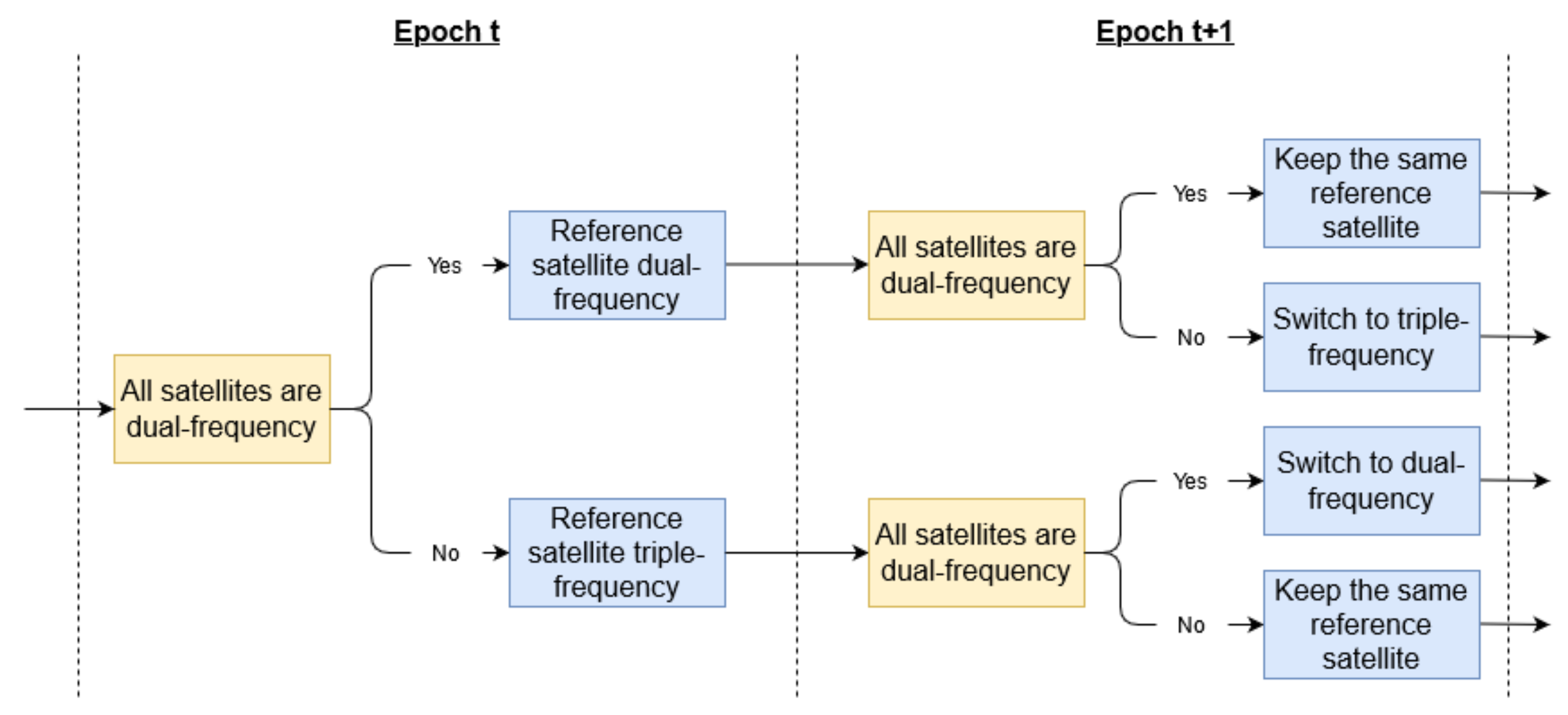
The fact that the datum of the carrier-phase measurements is set by the reference satellite’s ambiguities means that the reference satellite choice must depend on the number of frequencies available for the constellation in question. Indeed, for the GPS constellation for example, if only dual-frequency satellites are visible to the receiver, then the reference satellite can be dual-frequency. However, as soon as a triple-frequency satellite is included in the processing, the reference satellite must be switched to one of the triple-frequency satellites to set the datum on the third frequency. The reference satellite must therefore contain as many frequencies as the maximum number of frequencies in its constellation. A summary of the strategy of reference satellite choice is provided in Figure 1. The summary only focuses on the impact of the number of frequencies on the reference satellite choice. Other parameters need to be taken into account when making the choice, such as choosing a satellite that was processed for a long enough time that its ambiguities are correctly estimated, and a satellite that has the highest elevation angle and signal-to-noise ratio among the available satellites, etc. Note that another approach can be used when setting the datum for phase measurements, as the datum on each frequency does not have to be set by the same satellite. As a consequence, instead of requiring the reference satellite to have as many frequencies as processed for its constellation, the datum on the first two frequencies can be set by a dual-frequency satellite, while the datum on the third frequency can be set by one of the triple-frequency satellites’ third frequency phase measurement.
2.2. Data and Processing
The algorithms described above are tested on two sets of data. One worldwide set of stations from the International GNSS Service (IGS) is chosen to assess the global performance of the algorithms, as well as to draw conclusions on areas of improvement. Another set of kinematic data were collected by placing a geodetic receiver on a car and driving in a surburban environment, where the purpose is to highlight the benefits from the additional frequencies to achieve instantaneous precise positioning in the kinematic case.
Figure 2 shows the network of stations used in the processing. 32 IGS stations were randomly chosen, the only constraints being that they should track all four major GNSS constellations on up to three frequencies. The stations were processed in 1-h-long independent datasets from day 70–77 of 2021, with a sample interval of 30 s, leading to a total of 6137 individual datasets after filtering out some datasets with missing epochs of observations. This sample size is considered to be significant enough to allow generalization of the conclusions and results to assess the performance of the proposed algorithms and to analyze the impact of the fixing of the third frequency’s ambiguities.
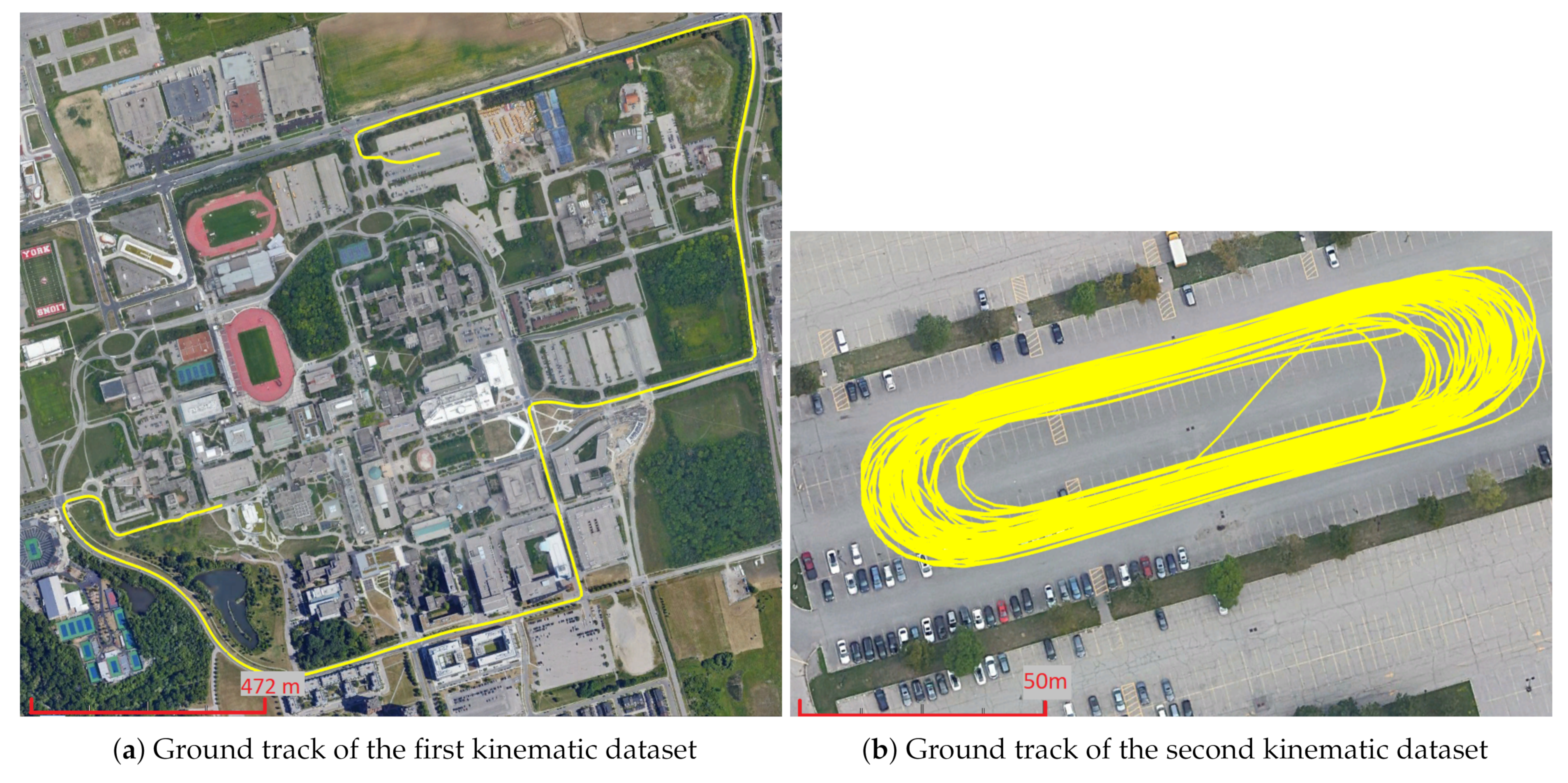
The kinematic testing is done with a geodetic NovAtel PwrPak7 receiver, which was placed, along with its antenna, on a rack on top of the roof of a car. The car was driven to collect two separate datasets, with a sampling rate of 1 Hz: one dataset was collected by driving close to the York University campus in Toronto, Canada on DOY 337, 2020, and a second parking lot dataset where the car was driven in an open-sky parking lot on DOY 151, 2021. The ground tracks of the two datasets are shown in Figure 3. A second NovAtel PwrPak7 receiver was used as a base station at a surveyed location and an RTK (Real Time Kinematics) solution was generated as a reference solution using the commercial RTK software NovAtel Inertial Explorer. The baseline for both datasets was kept under 5 km.
The constellations being processed are GPS, GLONASS, Galileo, and BeiDou-2, with ambiguities being resolved for GPS, Galileo, and BeiDou-2. BeiDou-3 was not included in the processing due to satellite bias corrections not being widely available yet, making ambiguity resolution impossible. In terms of frequencies, L1, L2, and L5 were processed for GPS, G1, and G2 for GLONASS, E1, E5b, and E5a for Galileo, and B1-2, B2b, and B3 for BeiDou-2.
Although the IGS stations are static, they are processed as if they were kinematic without imposing constraints on the receiver’s dynamics. The stations’ position coordinates are estimated using process noise of 100 km/h. The same process noise is also used for the two kinematic datasets. For receiver biases, although they tend to only vary by a few nanoseconds over a day, their behaviour depends on the temperature, location, and quality of the receiver, as they could reach relatively high variations [23,24,25]. To be cautious, the DCM does not make assumptions on the behaviour of biases and treats them as clock-like terms, leading to all receiver-related states being estimated as clock-like terms and treated as white noise processes. Receiver and satellite antenna corrections are corrected for using the IGS14 ANTEX file [26]. Because the GPS L5 satellite antenna corrections are not included in the ANTEX file, the corrections on L2 are applied on L5 measurements. A complete description of the processing strategies adopted for the various estimated parameters is provided in Table 2. The processing was performed with the in-house PPP engine developed at York University’s GNSS lab [27,28].
To allow for PPP processing in general, and ambiguity resolution specifically, satellite products are required. The products used in this work are provided by Centre National d’Etudes Spatiales (CNES), in RINEX format. The products are ultra-rapid but provided in post-processing, meaning that the products would be the same as those used by a real-time engine. However, instead of doing the processing in real-time, it is done in post-processing with real-time products. Therefore, the performance in this work is expected to be same as the performance a real-time user would get. This fact is promising and increases the importance of the results in this manuscript, as it allows the assessment of the attainable performance for real-time applications, for example, autonomous vehicles, or any application interested in real-time use of PPP.
As the model is based on uncombined processing of measurements, the float ambiguities are estimated in their uncombined state. These ambiguities, together with their corresponding covariance matrix, are fed into the mLAMBDA (modified Least-squares AMBiguity Decorrelation Adjustment) method [31], which is a more computationally efficient version of the LAMBDA method introduced in [32]. The uncombined ambiguities are therefore fixed to their integer values based on the float ambiguities and their covariances on each epoch, and all the estimated states are updated based on the fixed integer ambiguities. For each dataset, the fixing of ambiguities is attempted from the first epoch of processing, with the fixing only being attempted on satellites with elevation angles above 15 degrees. The reason for eliminating satellites below that threshold is that such satellites would be expected to have more multipath, ionospheric refraction and measurement noise, which would affect the estimation of those satellites’ ambiguities. The fixing of the ambiguities is validated using a standard ratio test.
3. Results
The results section consists of two main parts. First, results from the network of IGS stations are analyzed through a comparison of dual-frequency, triple-frequency, and mixed dual-/triple-frequency results. The latter results (simultaneous processing of dual-frequency and triple-frequency satellites) are analyzed in more detail in terms of convergence time and accuracy, with sample results from a single dataset being provided as well. The second part of the results section focuses on the kinematic vehicle datasets and analyzes the performance that can be achieved in real kinematic scenarios. Results are discussed as they are presented, and where applicable, compared to published research.
3.1. Performance Comparison with Dual-, Triple-, and Mixed Dual-/Triple-Frequency Processing
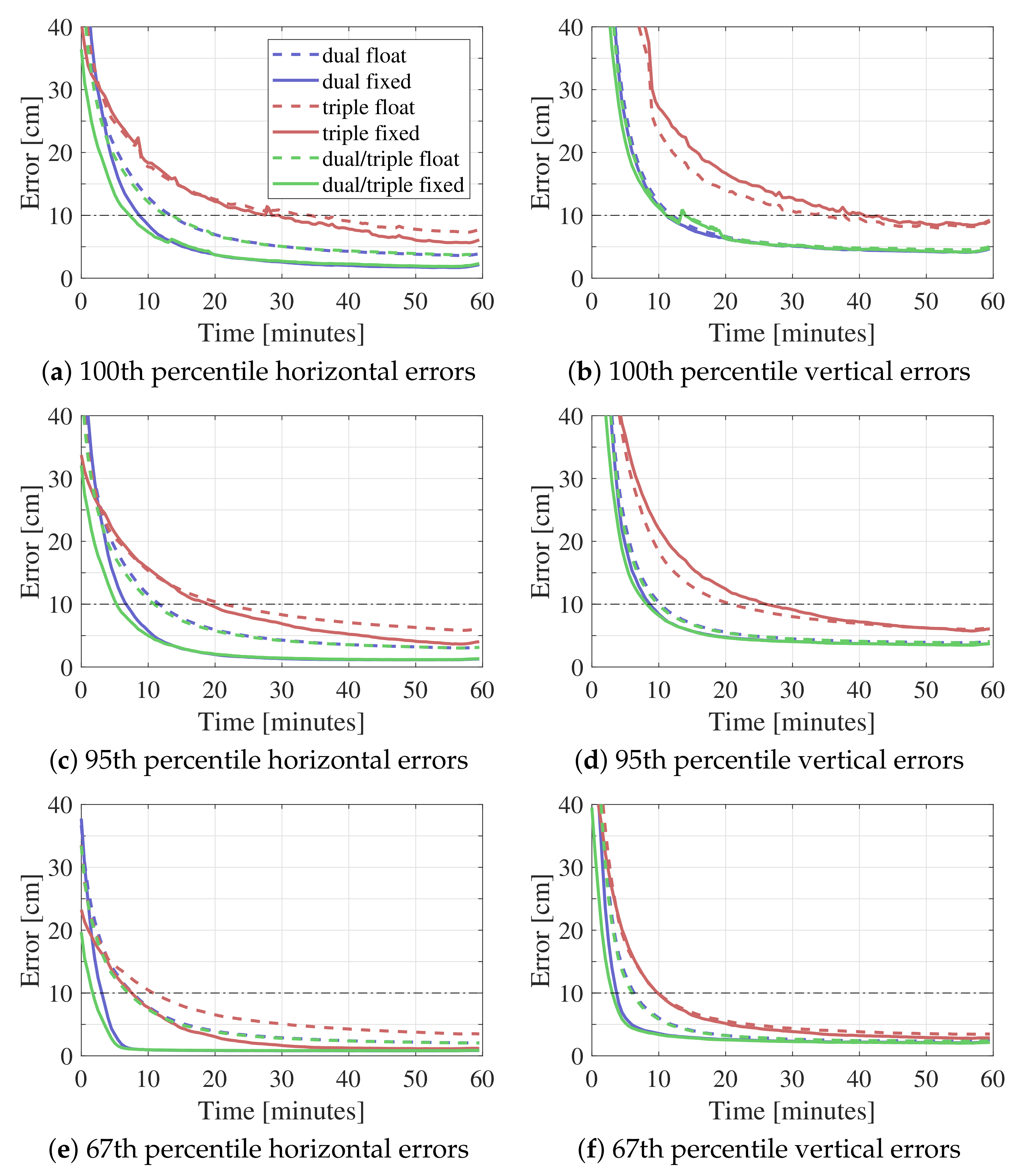
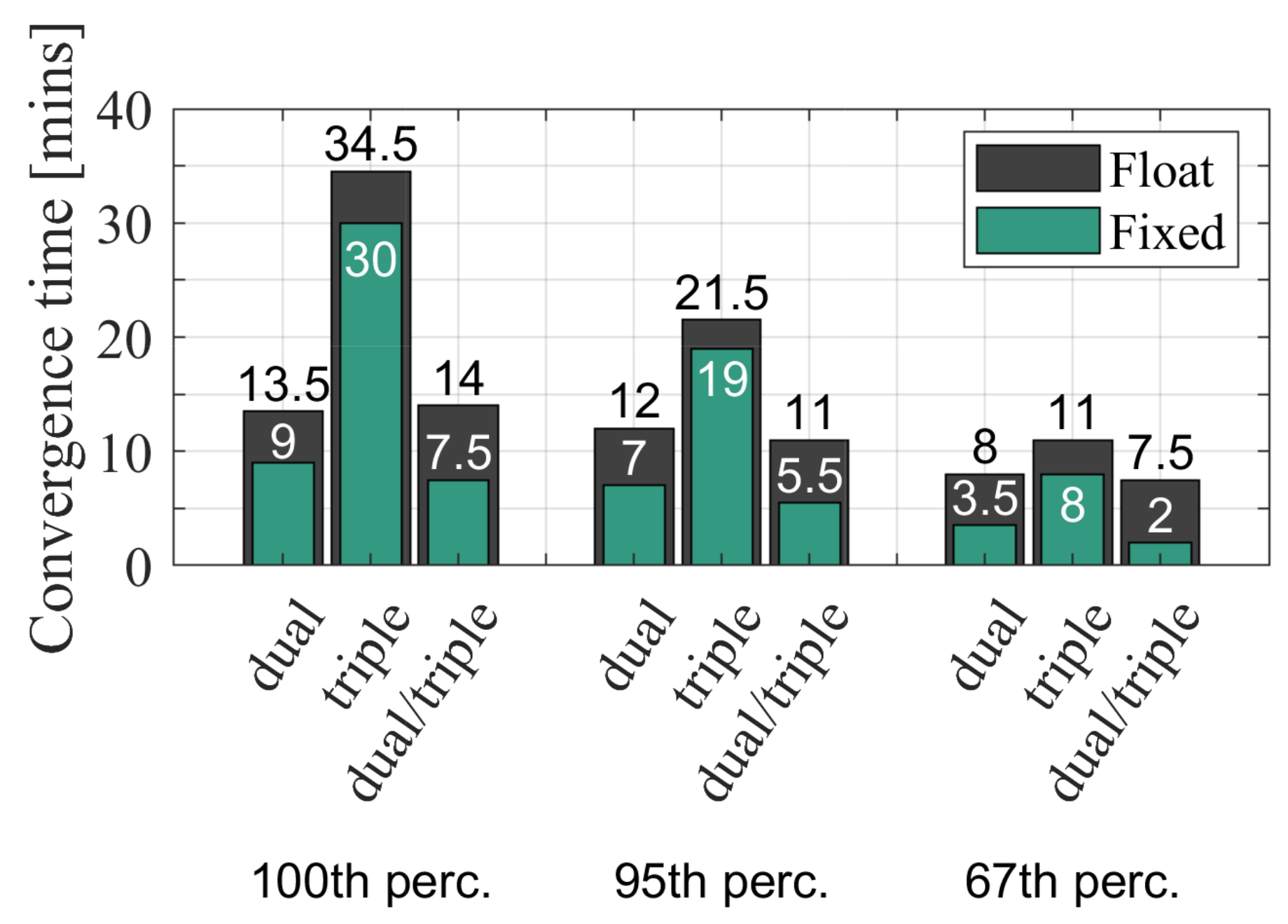
To assess the impact of the frequency combinations on the PPP and PPP-AR results, the 100th, 95th, and 67th percentiles are computed for both float and fixed horizontal and vertical errors. The results are presented in Figure 4 in the form of time series. The horizontal dashed lines refer to the convergence threshold defined in this work as the time it takes to reach and settle below a 10 cm horizontal error for the rest of the dataset. The horizontal convergence times corresponding to Figure 4 are summarized in Figure 5.
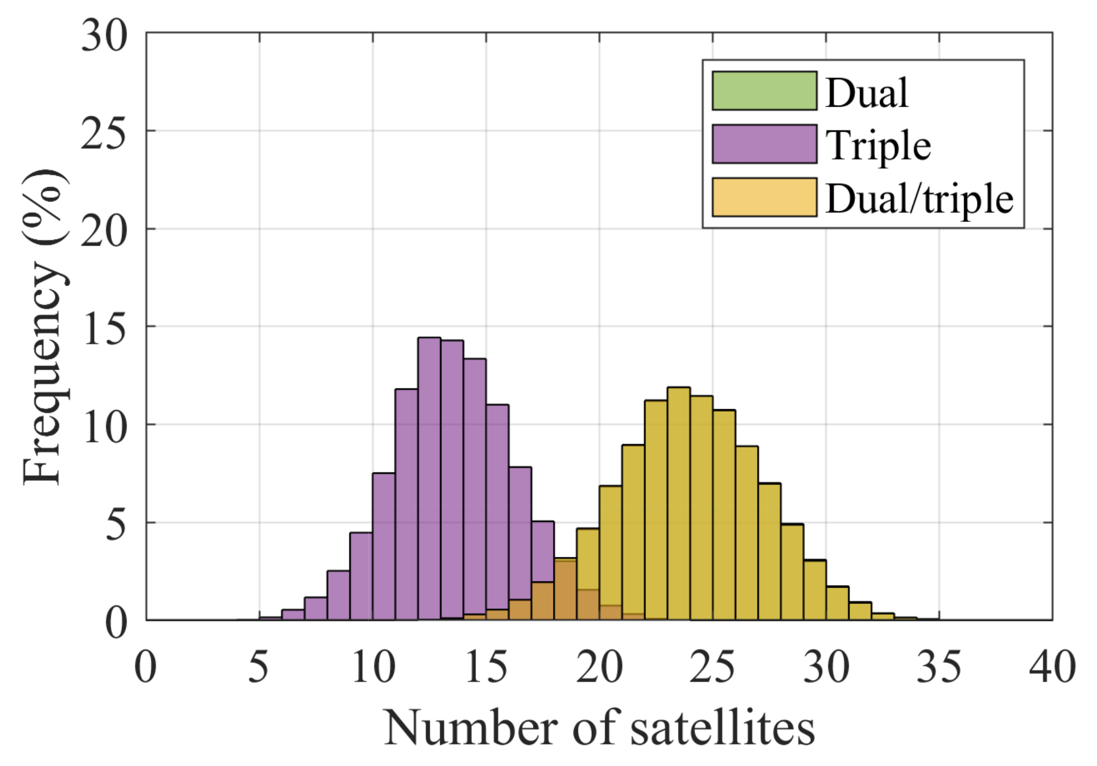
Multiple observations can be made from Figure 4 and Figure 5. Firstly, let us discuss the triple-frequency results to highlight the importance of processing and fixing a combination of dual- and triple-frequency satellites. The triple-frequency results appear to perform worse than dual-frequency and dual-/triple-frequency results, for both float and fixed solutions. The reason behind this behaviour is that the triple-frequency result excludes any satellite that does not have measurements on all three frequencies simultaneously. This exclusion means that only GPS-IIF and GPS-III satellites are processed for example, and GLONASS is not included in the processing as all of its satellites are dual-frequency. The histogram of the number of satellites for all three frequency combinations is shown in Figure 6. The graph is based on all epochs from all datasets, and indicates the distribution of the number of satellites overall. Given that the dual-/triple-frequency processing mode includes both dual- and triple-frequency satellites, the number of satellites distributions between the dual-frequency mode and dual-/triple-frequency mode are completely overlapping. On average, there are 13 satellites being processed in the triple-frequency mode, as opposed to 23 satellites in dual-(/triple-)frequency mode. This discrepancy in the number of satellites explains the worse performance in the triple-frequency-only results.
The triple-frequency results show worse performance from the AR solution at the 100th and 95th percentiles. The reason is that there are certain datasets for which a very low number of satellites is being tracked on all three frequencies simultaneously, leading to poor satellite geometry as well. Some of the problematic datasets are removed in the 95th percentile results, while most are removed when looking at the 67th percentile. The latter shows a decrease in the horizontal convergence time from 11 min for the float solution to 8 min for the fixed solution. The convergence time of the vertical solution was not impacted by AR, owing to the limited impact of AR on the vertical component.
When comparing the dual-frequency and mixed dual-/triple-frequency results, the addition of the third frequency does not seem to have any significant impact on the float solutions. Indeed, when comparing the dual-frequency and dual-/triple-frequency results, both float solutions have centimetre or even millimetre-level differences at all percentiles for both the horizontal and vertical components. This observation hints that the additional pseudorange and carrier-phase measurements do not provide significantly new information that would help the estimation of the various PPP states, as opposed to, e.g., adding a satellite to the processing, which would improve the satellite geometry and provide a new set of independent measurements.
However, despite the third frequency having a limited impact on the float solutions, its impact on the fixed solutions is more noticeable. Adding a third frequency to the dual-frequency fixed solutions improves performance, especially when it comes to the convergence of the solution. At the 100th percentile for example, not only does the horizontal convergence time decrease from 9 min to 7.5 min, but the initial errors decrease as well from 60 cm to 36 cm on the first epoch. The same levels of improvement are noticed at lower percentiles for the horizontal error, with the convergence time decreasing from 7 min to 5.5 min at the 95th percentile, and from 3.5 min to 2 min at the 67th percentile. The initial horizontal error decreases from 55 cm to 32 cm at the 95th percentile, and from 38 cm to 20 cm at the 67th percentile. The improvements in the fixed solution with the addition of the third frequency are attributed to the fixing becoming more reliable. Indeed, the ambiguities from the same satellite are correlated, which means that adding a third ambiguity for a satellite would lead to more reliable and accurate fixing of the ambiguities, as was similarly discussed in [33]. The impact of the third frequency on the ambiguity success rate for one of the kinematic datasets will be discussed in Figure 10.
In terms of the vertical component, the addition of the third frequency appears to have a limited effect on both the float and fixed solutions. For the float solutions, millimetre-level differences are seen between dual-frequency and mixed dual-/triple-frequency solutions. As described above for the horizontal solutions, this behaviour is attributed to the limited information provided by the third frequency to the state estimation. The improvements from the third frequency come from the addition of another ambiguity to fix, which is correlated to the first and second frequency ambiguities. However, its effect is very limited for the vertical component. The vertical convergence time at the 100th percentile decreases from 11.5 min to 11 min, while decreasing from 9 min to 8.5 min at the 95th percentile, and from 4 min to 3.5 min at the 67th percentile. The limited impact of AR on the vertical component’s convergence was also noticed in [19,34]. However, there are still improvements that can be noticed in the initial epochs, as the third frequency helps reduce the vertical errors before convergence. For instance, at the 100th percentile, the dual-frequency solution’s 124 cm initial error decreases to 90 cm with the dual-/triple-frequency solution. At the 95th percentile, the initial error decreases from 109 cm to 78 cm, while it decreases at the 67th percentile from 62 cm to 40 cm.
3.2. Mixed Dual-/Triple-Frequency Performance Analysis
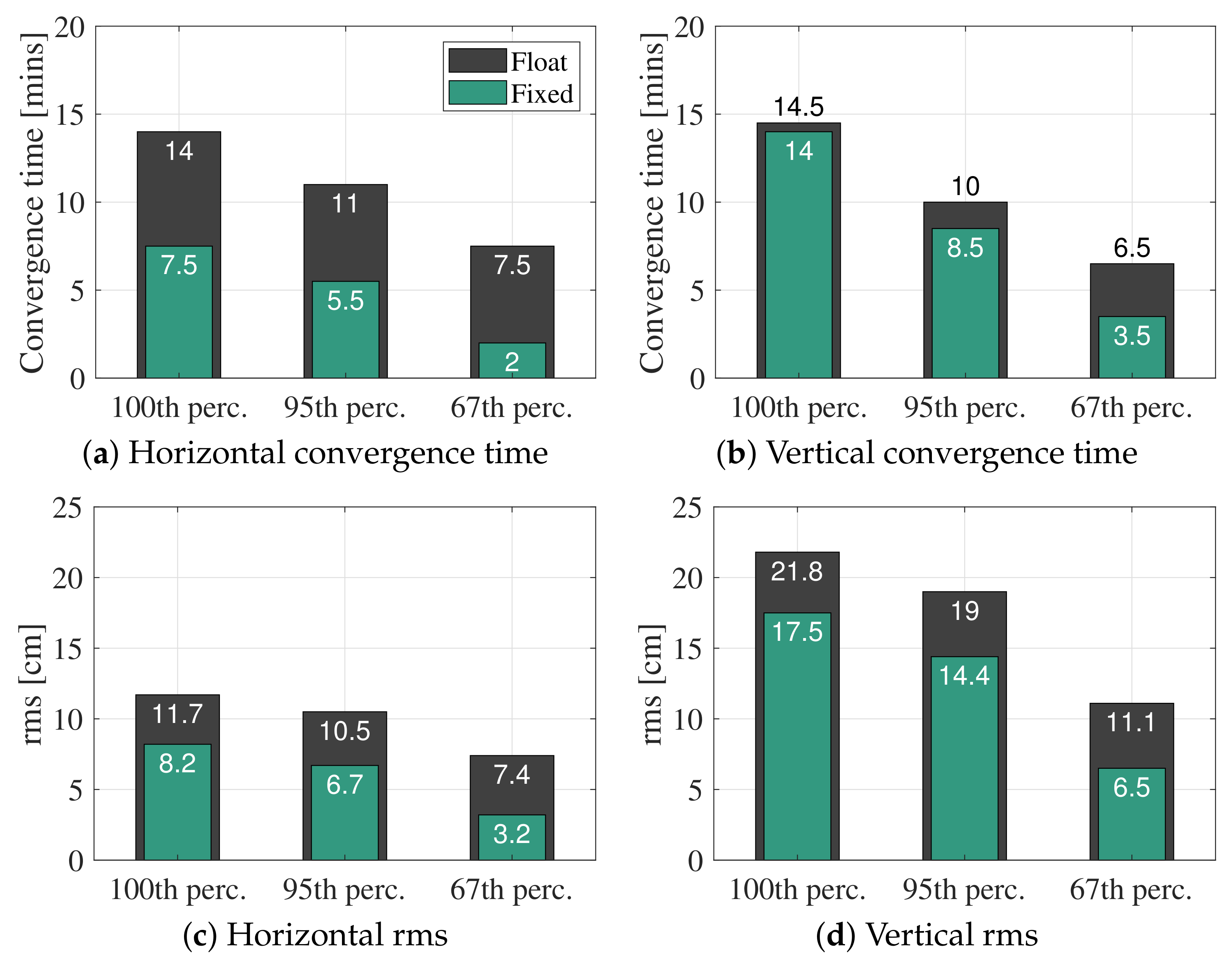
The previous section showed the benefits of simultaneously processing and fixing dual- and triple-frequency satellites. The current section focuses on the dual- and triple-frequency solution and analyzes its convergence time and accuracy performance in more detail. The horizontal and vertical convergence time and rms (root mean square error) for the dual-/triple-frequency solution are summarized in Figure 7.
As discussed in the previous section, looking at lower percentiles eliminates outlier solutions and gives a better idea on the distribution of the performance. For instance, the benefits of ambiguity resolution on up to three frequencies are clear on the horizontal convergence time. When fixing ambiguities, at the 1-sigma (67th percentile), the solutions converge to and stay below one decimetre within 2 min, with a improvement compared to that of the float solution. This result shows that it is possible to approach RTK levels of performance in terms of convergence time using only global corrections. Horizontal accuracy is also significantly improved as, at the 1-sigma (67th percentile), the rms reaches 3.2 cm. Note that this rms value is computed over the whole hour of processing and that it includes the initial convergence period. The accuracies after convergence are below 1 cm. These results could be improved with the inclusion of BeiDou-3, as well as the fourth Galileo frequency. However, the effect of AR is limited when it comes to the vertical component when looking at the 100th and 95th percentiles, as the improvements to the convergence time and rms are not as significant as for the horizontal component. Though at the 67th percentile, the vertical convergence time sees a improvement to reach 3.5 min. Similar conclusions are valid for the vertical rms, as the vertical positions are not as accurate as the horizontal ones. The better performance of the horizontal metrics is attributed to the fact that it is harder to estimate the vertical component due to the visible satellites all being distributed above the antenna (and the surface of the Earth).
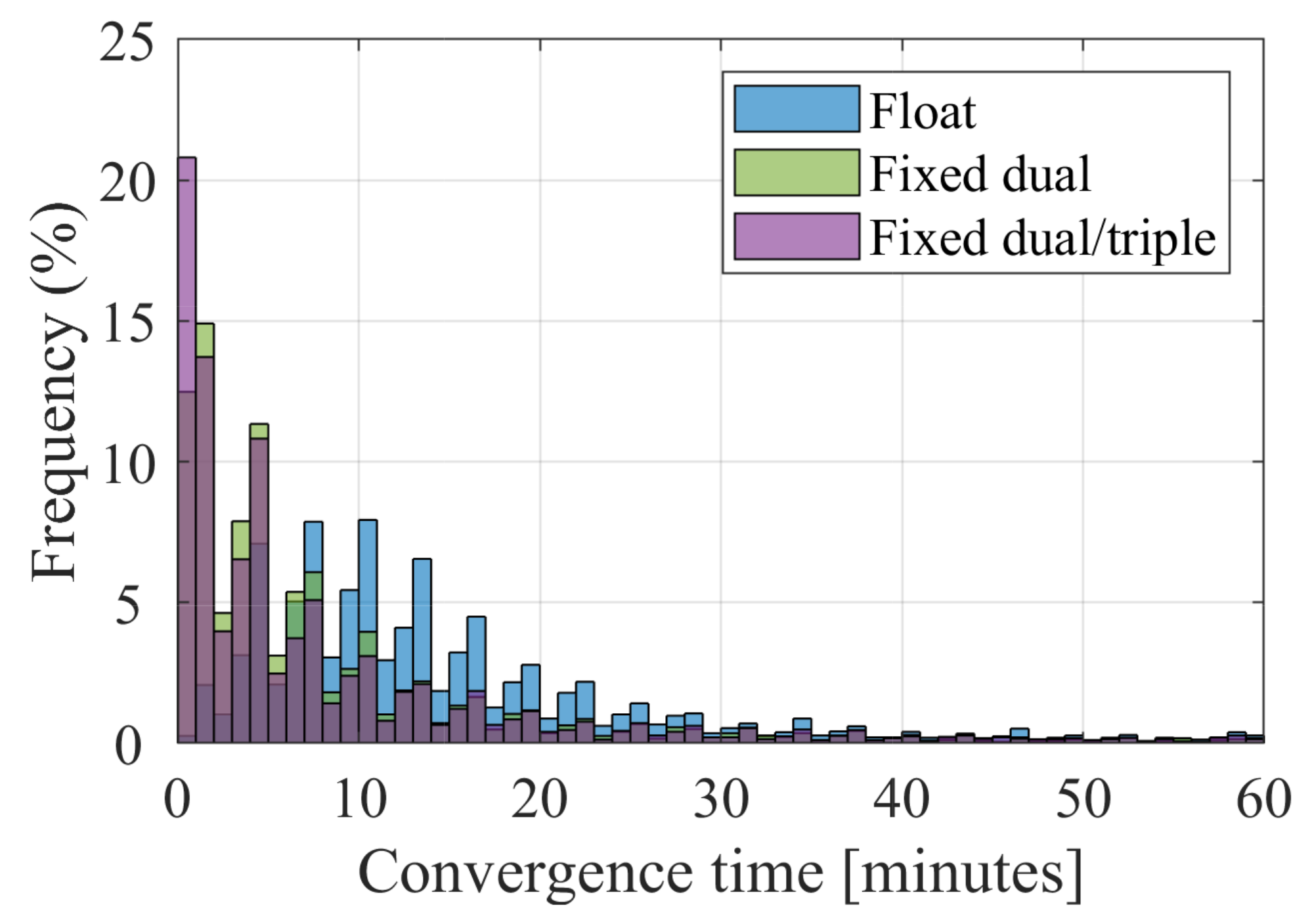
To understand the effect of AR and of the third frequency at the dataset level, Figure 8 shows the distribution of the convergence time based on all the datasets. Only one float histogram is shown, as the performance of both dual-frequency and mixed dual-/triple-frequency float solutions is very similar.
Figure 8 shows clear improvements when fixing ambiguities compared to the float solution: the histograms get shifted to the left of the x-axis, with datasets converging sooner and with the mean of the histogram becoming smaller. A large portion of the fixed results converge within the first few minutes, as opposed to the float results, for which the majority converge within 10 min. More specifically, only of float solutions converge instantaneously, compared to for the fixed dual-frequency solutions, and for the dual-/triple-frequency solutions. Similarly, only of float solutions converge within a minute, as opposed to for the fixed dual-frequency solutions, and for the dual-/triple-frequency solutions. These results show that fixing ambiguities on as many frequencies as possible brings PPP closer to global instantaneous convergence, as fixing more frequencies leads to faster convergence at the dataset level. To further highlight the impact of the third frequency at the dataset level, one sample result is shown in Figure 9 for station GODS in Greenbelt, USA.
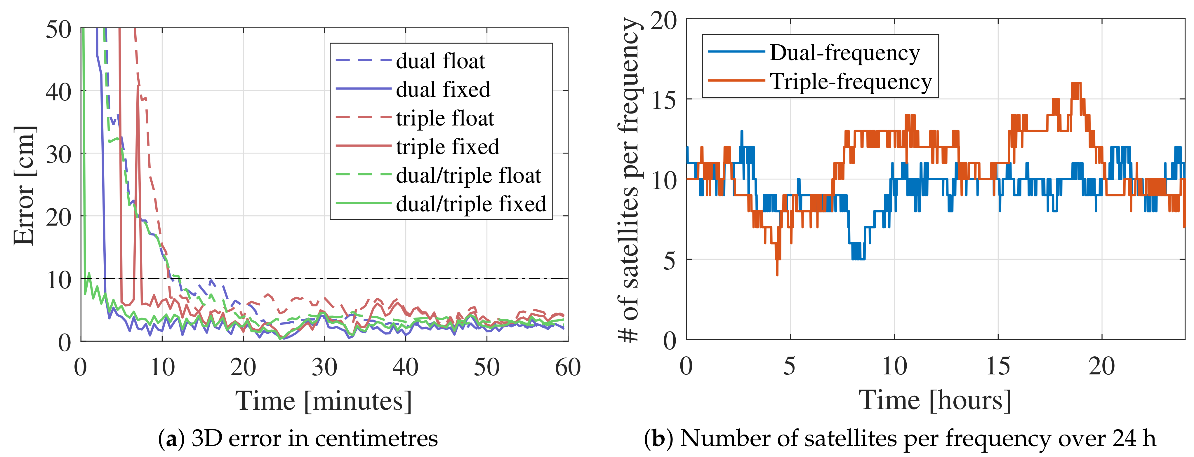
First, Figure 9 shows the similar performance between both dual-frequency and dual-/triple-frequency float solutions. Both solutions are overlapping with minimal differences, as was noticed in the average results using all datasets. The triple-frequency solution appears to perform worse than its dual(/triple)-frequency counterpart. As was explained in Figure 6, the reason behind this difference is the fewer number of satellites broadcasting on three frequencies. Figure 9b shows the number of satellites broadcasting on two and three frequencies and the evolution of the numbers over one day. In the case of triple-frequency processing, all dual-frequency-only satellites are rejected, leading to the number of satellites corresponding to the orange line and dropping as low as 4 satellites at around 4 am. Including both dual- and triple-frequency satellites leads to the number of satellites being the sum of both blue and orange graphs.
When looking at the fixed solutions, the triple-frequency solution performs the worst out of the three, as it uses a lower number of satellites. However, when comparing dual-frequency and dual-/triple-frequency results, the benefits of the third frequency become obvious. The 3D convergence time of the dual-/triple-frequency solution reaches 1.5 min, compared to 3 min for that of the dual-frequency solution. This reduction in the convergence time is a direct consequence of the third frequency, since it helps quicken the correct fixing of the ambiguities due to the correlation between ambiguities from the same satellite. After convergence, all accuracies are relatively similar, showing that most of the benefits from the additional frequency are in the form of faster convergence and smaller position errors before convergence. The fluctuations in the solutions after convergence are due to the receiver coordinates being estimated in kinematic mode, leading to noise affecting the position estimates.
3.3. Kinematic Automotive Data Results
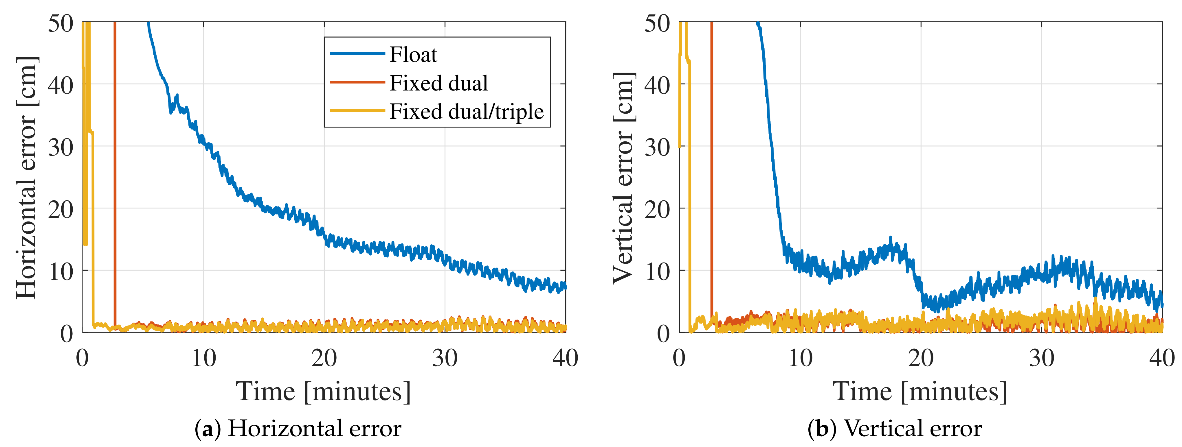
While it is important to assess the performance of the proposed algorithm with static IGS data, it is equally important to do the assessment with various test scenarios. In this case, the focus is on kinematic data using geodetic hardware. Two datasets are collected, as shown with their ground tracks in Figure 3 and processed in dual-frequency and dual-/triple-frequency modes. The triple-frequency processing is omitted as its limitations were established in the previous sections. Figure 10 shows the results for the first suburban dataset.
Figure 10a,b show the improvements from both ambiguity resolution and the third frequency. The horizontal float solution (being the same in both dual-frequency and dual-/triple-frequency) converges below a decimetre after 24.5 min and has an overall rms of 12.5 cm. These statistics are greatly improved when fixing ambiguities in dual-frequency mode, as the convergence time decreases to 0.5 min, with an overall rms of 3.2 cm. The results improve further when fixing the third frequency, as instantaneous convergence is achieved with an overall rms of 1.5 cm. This level of performance is comparable to RTK and is impressive given that only ultra-rapid global orbits, clocks and biases are used in the processing. The improvements from the third frequency in this case appear in the form of correct fixing in the initial epochs when the ambiguities tend to not be estimated well enough to be fixed correctly. This impact on the correct fixing of ambiguities is shown in Figure 10d which shows the ambiguity success rate [35] for both frequency combinations: adding a third frequency leads to an increase of the success rate of the ambiguities, especially during the initial epochs of processing, allowing for instantaneous convergence.
As was the case with the IGS data, the vertical component in this case is not estimated as well as the horizontal component. The variations in the float solution, which has an rms of 7.8 cm, are reduced when fixing the ambiguities, as the rms of the dual-frequency fixed solution is reduced to 4.7 cm, to be further reduced to 3 cm for the dual-/triple-frequency fixed solution. The higher variations that are seen in both horizontal and vertical errors after 20 min are due to the car being driven in a high-multipath area, with buildings on both sides of the road. The effect of the signal blockages on the number of satellites can be seen in Figure 10c.
While the effect of the third frequency is relatively limited for this first dataset, it is more noticeable when looking at the second dataset, which was collected in an open-sky parking lot. The results from the processing are summarized in Figure 11.
In the same fashion as for the first kinematic dataset, only one float solution is shown due to both float solutions being very similar in performance. The horizontal float solution takes a relatively long time of 35 min to converge to the decimetre-level in this case with an overall rms of 36.4 cm. Similarly to the first dataset, fixing the dual-frequency ambiguities allows for better accuracies to be reached sooner, as the solution converges within 2.7 min, with an accuracy of 32.4 cm. The relatively high rms value is due to the errors being relatively high before convergence, as the rms after convergence is 1 cm. The convergence time is further decreased to 51 s when fixing the third frequency as well, with a total rms of 5 cm, and an rms after convergence of 1 cm. A similar performance is noticed with the vertical component, as the rms after 5 min reaches 17 cm, 1.7 cm, and 1.9 cm for the float, fixed dual-frequency, and fixed dual-/triple-frequency solutions, respectively, with convergence times of 34 min, 2.7 min, and 51 s, respectively.
4. Discussion
The analysis of the impact of the third frequency on PPP and PPP-AR with a flexible model was not shown in the literature. Analysis involving multiple frequencies tends to be focused on comparing only satellites with the same number of frequencies (for example Galileo, or GPS-IIF) [9,17,18,36]. In this manuscript, a comprehensive performance analysis is done by not rejecting satellites that only broadcast on two frequencies, allowing for the processing of many healthy satellites that would be otherwise rejected. This flexible processing allows for a realistic assessment of PPP performance in the current multi-GNSS multi-frequency context, and it proves the benefits of including as many satellites as available, as PPP performance is further improved compared to a solution where only dual-frequency or only triple-frequency satellites are processed.
The impact of simultaneous processing and fixing of dual-frequency and triple-frequency satellites is demonstrated. On the one hand, given that not all satellites broadcast on three frequencies, allowing for the mix of dual- and triple-frequency measurements leads to an increase of the number of processed satellites, as opposed to rejecting satellites without a third frequency. On the other hand, the addition of a third frequency is shown to improve the PPP-AR solutions. This improvement is attributed to the fixing becoming more reliable. For instance, the addition of the third frequency allows for the formation of the extra-widelane (EWL) ambiguity, which has metre-level wavelength and can be fixed instantaneously. Being able to fix the EWL helps in the fixing of the widelane ambiguity, which in turn helps the fixing of the narrowlane. Ref. [37] demonstrated the improvements that the third frequency ambiguities bring to the correct fixing of the narrowlane ambiguities based on simulated GPS data.
Limited impact is noticed from the addition of a third frequency on the PPP float solutions. Similar observations on the limited effect of additional frequencies on the float solution were noticed in [36] using the BeiDou constellation and the effect of the third frequency was expected to be more significant in the case of poor measurement quality. The limited effect of the third frequency was also mentioned in [19], where the Galileo constellation was used, and in [9] where multiple constellations were processed. Despite this limited effect of the third frequency measurements on the float solutions, it is important not to reject any satellite with only two frequencies, as that would lead to the performance seen in the triple-frequency results.
The proposed algorithms are also tested on datasets collected with geodetic hardware placed on a car. The vehicle results, shown in the previous section, demonstrate the benefits of processing a mix of dual- and triple-frequency measurements from all four major GNSS constellations. Doing so opens the door to instantaneous precise positioning that only requires globally estimated satellite products. The analysis of the impact of PPP-AR in general, and multi-frequency PPP-AR specifically, on vehicle datasets is limited in the literature. For instance, ref. [38] analyzed the performance of a triple-frequency four-constellation solution where only triple-frequency satellites were processed and where the average number of satellites was 12. The solution achieved rms of 0.29 m, 0.35 m, and 0.77 m in the east, north, and up components, respectively, although only widelane and extra-widelane ambiguities were fixed. Ref. [39] analyzed the impact of an inertial navigation system (INS) on PPP-AR re-convergence using GPS and GLONASS on two frequencies, and was able to achieve convergence (time to first fix (TTFF)) in approximately 30 min. Ref. [40] achieved 0.23 m, 0.27 m, and 0.46 m rms in the east, north, and up components, though only the BeiDou constellation was used, and only widelane and extra-widelane ambiguities were fixed. This brief literature review highlights the importance of the kinematic results in this manuscript, as narrowlane ambiguities are fixed in addition to widelane and extra-widelane, in a model that is able to process and fix dual- and triple-frequency measurements from all major GNSS constellations. This flexibility and capability allow for instantaneous centimetre-level positioning within seconds to tens of seconds.
5. Conclusions
Ambiguity resolution proved to be an important tool to level-up PPP towards instantaneous centimetre positioning. With all the frequencies being broadcast from all the major constellations in orbit, ambiguity resolution can be made to be more successful, especially during initial epochs of processing, bringing the PPP convergence time down. In this manuscript, a flexible multi-GNSS triple-frequency uncombined Decoupled Clock Model is introduced. Given that all satellites do not broadcast on three frequencies, as some only support two frequencies, the DCM was altered to be able to process and fix both dual-frequency and triple-frequency satellites simultaneously. This simultaneous processing requires careful handling of the PPP states and of the reference satellite, as the latter has to contain as many frequencies as the maximum number of frequencies being available in all satellites.
The algorithm was first tested on static IGS data processed in kinematic mode, which showed that convergence below a decimetre for the horizontal component is possible within 2 min of processing at the 1-sigma (67th percentile). After convergence, the horizontal rms reaches 1 cm, while the vertical rms reaches 2 cm. The third frequency is found to have a limited impact on the float solution, as most of its benefits are in the form of more successful ambiguity fixing during convergence, allowing for centimetre accuracies to be achieved faster; though the effect of both ambiguity resolution and the third frequency is relatively limited when it comes to the vertical component. The algorithm was also tested on kinematic data collected by driving a car in two different scenarios. The results show that quasi-instantaneous centimetre positioning is possible even with a moving receiver, as one dataset reached and stayed at 1 cm horizontal error for the whole duration of the dataset, while the other dataset managed to do so after 51 s. Though it was noticed that the environment can still have an impact on the level of noise in the position estimates, in high-multipath areas, for example.
The work in this manuscript is novel in the fact that, rather than discarding satellites broadcasting only on two frequencies as is typically done, those satellites are included in the processing, alongside triple-frequency satellites. Doing so allows for improvements in the geometry, but also more reliable fixing of ambiguities. Having this flexible processing is shown to provide significant improvements compared to a dual-frequency-only or a triple-frequency-only solution. The importance of this work is confirmed by the results, as they show that global instantaneous centimetre-level positioning is possible, even with vehicle data. Indeed, these results are based on ultra-rapid products generated from a global network, without the use of any local information. These results open the door for PPP to be used in real-time applications that require precise positioning, such as autonomous driving.
The results are expected to further improve by adding additional frequencies, such as Galileo’s E6 signal, or with the addition of BeiDou-3, which are all intended as future work. By doing so, it is expected that the results would improve even further, with more datasets being able to converge instantaneously. When it comes to kinematic datasets, the results can be further improved through careful handling of the multipath errors in areas where it would affect the positioning accuracy.
Author Contributions
Conceptualization, N.N. and S.B.; methodology, N.N.; software, N.N.; investigation, N.N.; writing—original draft preparation, N.N.; writing—review and editing, N.N. and S.B.; visualization, N.N.; supervision, S.B. funding acquisition, S.B. All authors have read and agreed to the published version of the manuscript.
Funding
This article/publication is part of the project GISCAD-OV that received funding from the European GNSS Agency under the European Union’s Horizon 2020 research and innovation program under grant agreement No. 870231. This research was also funded by York University.
Data Availability Statement
GNSS observation data are provided by the Multi-GNSS Experiment (MGEX) from the International GNSS Service (IGS). Satellite products are provided by CNES. All the data and products are publicly available through the respective organizations’ websites.
Conflicts of Interest
The authors declare no conflict of interest.
References
- Zumberge, J.; Heflin, M.; Jefferson, D.; Watkins, M.; Webb, F. Precise point positioning for the efficient and robust analysis of GPS data from large networks. J. Geophys. Res. Solid Earth 1997, 102, 5005–5017. [Google Scholar] [CrossRef] [Green Version]
- Kouba, J.; Héroux, P. Precise point positioning using IGS orbit and clock products. GPS Solut. 2001, 5, 12–28. [Google Scholar] [CrossRef]
- Takasu, T.; Yasuda, A. Kalman-filter-based integer ambiguity resolution strategy for long-baseline RTK with ionosphere and troposphere estimation. In Proceedings of the 23rd International Technical Meeting of the Satellite Division of the Institute of Navigation (ION GNSS 2010), Portland, OR, USA, 21–24 September 2010; pp. 161–171. [Google Scholar]
- Odolinski, R.; Teunissen, P.; Odijk, D. Combined GPS+ BDS for short to long baseline RTK positioning. Meas. Sci. Technol. 2015, 26, 045801. [Google Scholar] [CrossRef]
- Bisnath, S. PPP: Perhaps the natural processing mode for precise GNSS PNT. In Proceedings of the 2020 IEEE/ION Position, Location and Navigation Symposium (PLANS), Portland, OR, USA, 20–23 April 2020; pp. 419–425. [Google Scholar]
- Bisnath, S.; Gao, Y. Precise point positioning a powerful technique with a promising future. GPS World 2009, 20, 43–50. [Google Scholar]
- Nadarajah, N.; Khodabandeh, A.; Wang, K.; Choudhury, M.; Teunissen, P.J. Multi-GNSS PPP-RTK: From large-to small-scale networks. Sensors 2018, 18, 1078. [Google Scholar] [CrossRef] [PubMed] [Green Version]
- Collins, P.; Lahaye, F.; Heroux, P.; Bisnath, S. Precise point positioning with ambiguity resolution using the decoupled clock model. In Proceedings of the 21st International Technical Meeting of the Satellite Division of the Institute of Navigation (ION GNSS 2008), Savannah, GA, USA, 16–19 September 2008; pp. 1315–1322. [Google Scholar]
- Geng, J.; Guo, J.; Meng, X.; Gao, K. Speeding up PPP ambiguity resolution using triple-frequency GPS/BeiDou/Galileo/QZSS data. J. Geod. 2020, 94, 1–15. [Google Scholar] [CrossRef] [Green Version]
- Naciri, N.; Bisnath, S. Multi-GNSS Ambiguity Resolution as a Substitute to Obstructed Satellites in Precise Point Positioning Processing. In Proceedings of the 33rd International Technical Meeting of the Satellite Division of the Institute of Navigation (ION GNSS+ 2020), Virtual, 21–25 September 2020; pp. 2960–2971. [Google Scholar]
- Collins, P. Isolating and estimating undifferenced GPS integer ambiguities. In Proceedings of the Institute of Navigation, National Technical Meeting, San Diego, CA, USA, 28–30 January 2008; Volume 2, pp. 720–732. [Google Scholar]
- Collins, P.; Lahaye, F.; Bisnath, S. External ionospheric constraints for improved PPP-AR initialisation and a generalised local augmentation concept. In Proceedings of the 25th International Technical Meeting of the Satellite Division of the Institute of Navigation (ION GNSS 2012), Nashville, TN, USA, 17–21 September 2012; pp. 3055–3065. [Google Scholar]
- Banville, S.; Collins, P.; Zhang, W.; Langley, R.B. Global and regional ionospheric corrections for faster PPP convergence. Navig. J. Inst. Navig. 2014, 61, 115–124. [Google Scholar] [CrossRef]
- Aggrey, J.; Bisnath, S. Improving GNSS PPP convergence: The case of atmospheric-constrained, multi-GNSS PPP-AR. Sensors 2019, 19, 587. [Google Scholar] [CrossRef] [PubMed] [Green Version]
- Naciri, N.; Hauschild, A.; Bisnath, S. Exploring Signals on L5/E5a/B2a for Dual-Frequency GNSS Precise Point Positioning. Sensors 2021, 21, 2046. [Google Scholar] [CrossRef]
- Cai, C.; Gao, Y.; Pan, L.; Zhu, J. Precise point positioning with quad-constellations: GPS, BeiDou, GLONASS and Galileo. Adv. Space Res. 2015, 56, 133–143. [Google Scholar] [CrossRef]
- Li, X.; Liu, G.; Li, X.; Zhou, F.; Feng, G.; Yuan, Y.; Zhang, K. Galileo PPP rapid ambiguity resolution with five-frequency observations. GPS Solut. 2020, 24, 1–13. [Google Scholar] [CrossRef]
- Geng, J.; Guo, J. Beyond three frequencies: An extendable model for single-epoch decimeter-level point positioning by exploiting Galileo and BeiDou-3 signals. J. Geod. 2020, 94, 1–15. [Google Scholar] [CrossRef]
- Naciri, N.; Bisnath, S. An uncombined triple-frequency user implementation of the decoupled clock model for PPP-AR. J. Geod. 2021, 95, 1–17. [Google Scholar] [CrossRef]
- El-Mowafy, A.; Deo, M.; Rizos, C. On biases in precise point positioning with multi-constellation and multi-frequency GNSS data. Meas. Sci. Technol. 2016, 27, 035102. [Google Scholar] [CrossRef]
- Håkansson, M.; Jensen, A.B.; Horemuz, M.; Hedling, G. Review of code and phase biases in multi-GNSS positioning. GPS Solut. 2017, 21, 849–860. [Google Scholar] [CrossRef] [Green Version]
- Zhou, F.; Dong, D.; Li, P.; Li, X.; Schuh, H. Influence of stochastic modeling for inter-system biases on multi-GNSS undifferenced and uncombined precise point positioning. GPS Solut. 2019, 23, 1–13. [Google Scholar] [CrossRef]
- Abdelazeem, M.; Çelik, R.N.; El-Rabbany, A. MGR-DCB: A precise model for multi-constellation GNSS receiver differential code bias. J. Navig. 2016, 69, 698–708. [Google Scholar] [CrossRef] [Green Version]
- Zhang, B.; Teunissen, P.; Yuan, Y. On the short-term temporal variations of GNSS receiver differential phase biases. J. Geod. 2017, 91, 563–572. [Google Scholar] [CrossRef] [Green Version]
- Zhang, B.; Teunissen, P.; Yuan, Y.; Zhang, X.; Li, M. A modified carrier-to-code leveling method for retrieving ionospheric observables and detecting short-term temporal variability of receiver differential code biases. J. Geod. 2018, 93, 19–28. [Google Scholar] [CrossRef] [Green Version]
- Schmid, R.; Dach, R.; Collilieux, X.; Jäggi, A.; Schmitz, M.; Dilssner, F. Absolute IGS antenna phase center model igs08. atx: Status and potential improvements. J. Geod. 2016, 90, 343–364. [Google Scholar] [CrossRef] [Green Version]
- Aggrey, J. Precise Point Positioning Augmentation for Various Grades of Global Navigation Satellite System Hardware. Ph.D. Thesis, York University, Toronto, ON, Canada, 2019. [Google Scholar]
- Seepersad, G. Reduction of Initial Convergence Period in GPS PPP Data Processing. Ph.D. Thesis, York University, Toronto, ON, Canada, 2012. [Google Scholar]
- Kouba, J. Testing of global pressure/temperature (GPT) model and global mapping function (GMF) in GPS analyses. J. Geod. 2009, 83, 199–208. [Google Scholar] [CrossRef]
- Laurichesse, D.; Blot, A. Fast PPP convergence using multi-constellation and triple-frequency ambiguity resolution. In Proceedings of the 29th International Technical Meeting of the Satellite Division of the Institute of Navigation, ION GNSS+ 2016, Portland, OR, USA, 12–16 September 2016; Volume 3, pp. 2082–2088. [Google Scholar] [CrossRef] [Green Version]
- Chang, X.W.; Yang, X.; Zhou, T. MLAMBDA: A modified LAMBDA method for integer least-squares estimation. J. Geod. 2005, 79, 552–565. [Google Scholar] [CrossRef] [Green Version]
- Teunissen, J. The least-squares ambiguity decorrelation adjustment: A method for fast GPS integer ambiguity estimation. J. Geod. 1995, 70, 65–82. [Google Scholar] [CrossRef]
- Xiao, G.; Li, P.; Gao, Y.; Heck, B. A unified model for multi-frequency PPP ambiguity resolution and test results with Galileo and BeiDou triple-frequency observations. Remote Sens. 2019, 11, 116. [Google Scholar] [CrossRef] [Green Version]
- Shi, J.; Gao, Y. A troposphere constraint method to improve PPP ambiguity-resolved height solution. J. Navig. 2014, 67, 249–262. [Google Scholar] [CrossRef]
- Teunissen, P. Influence of ambiguity precision on the success rate of GNSS integer ambiguity bootstrapping. J. Geod. 2007, 81, 351–358. [Google Scholar] [CrossRef] [Green Version]
- Guo, F.; Zhang, X.; Wang, J.; Ren, X. Modeling and assessment of triple-frequency BDS precise point positioning. J. Geod. 2016, 90, 1223–1235. [Google Scholar] [CrossRef]
- Geng, J.; Bock, Y. Triple-frequency GPS precise point positioning with rapid ambiguity resolution. J. Geod. 2013, 87, 449–460. [Google Scholar] [CrossRef]
- Geng, J.; Guo, J.; Chang, H.; Li, X. Toward global instantaneous decimeter-level positioning using tightly coupled multi-constellation and multi-frequency GNSS. J. Geod. 2019, 93, 977–991. [Google Scholar] [CrossRef] [Green Version]
- Zhang, X.; Zhu, F.; Zhang, Y.; Mohamed, F.; Zhou, W. The improvement in integer ambiguity resolution with INS aiding for kinematic precise point positioning. J. Geod. 2019, 93, 993–1010. [Google Scholar] [CrossRef]
- Li, X.; Li, X.; Liu, G.; Yuan, Y.; Freeshah, M.; Zhang, K.; Zhou, F. BDS multi-frequency PPP ambiguity resolution with new B2a/B2b/B2a+ b signals and legacy B1I/B3I signals. J. Geod. 2020, 94, 1–15. [Google Scholar] [CrossRef]
Figure 1.
Reference satellite choice strategy when processing a combination of dual- and triple-frequency satellites.
Figure 1.
Reference satellite choice strategy when processing a combination of dual- and triple-frequency satellites.

Figure 2.
IGS stations used in processing.

Figure 3.
Ground tracks of datasets used in kinematic processing.

Figure 4.
Time series comparison of 100th, 95th, and 67th percentile horizontal and vertical errors for dual-frequency, triple-frequency, and mixed dual-/triple-frequency combinations both with and without ambiguity resolution. Horizontal dashed lines represent convergence threshold.
Figure 4.
Time series comparison of 100th, 95th, and 67th percentile horizontal and vertical errors for dual-frequency, triple-frequency, and mixed dual-/triple-frequency combinations both with and without ambiguity resolution. Horizontal dashed lines represent convergence threshold.

Figure 5.
Horizontal convergence time for dual-frequency, triple-frequency, and mixed dual-/triple-frequency results with and without AR at 100th, 95th, and 67th percentiles. Convergence time statistics correspond to results in Figure 4.
Figure 5.
Horizontal convergence time for dual-frequency, triple-frequency, and mixed dual-/triple-frequency results with and without AR at 100th, 95th, and 67th percentiles. Convergence time statistics correspond to results in Figure 4.

Figure 6.
Histogram of number of satellites being processed in dual-frequency, triple-frequency, and mixed dual-/triple-frequency processing. Graph is based on all epochs from all datasets. “dual” and “dual/triple” histograms are overlapping.
Figure 6.
Histogram of number of satellites being processed in dual-frequency, triple-frequency, and mixed dual-/triple-frequency processing. Graph is based on all epochs from all datasets. “dual” and “dual/triple” histograms are overlapping.

Figure 7.
100th, 95th, and 67th percentile horizontal and vertical convergence times and rms for solution combining dual-frequency and triple-frequency satellites, with and without AR.
Figure 7.
100th, 95th, and 67th percentile horizontal and vertical convergence times and rms for solution combining dual-frequency and triple-frequency satellites, with and without AR.

Figure 8.
Float, dual-frequency fixed, and mixed dual-/triple-frequency fixed histogram of horizontal convergence time of all processed datasets.
Figure 8.
Float, dual-frequency fixed, and mixed dual-/triple-frequency fixed histogram of horizontal convergence time of all processed datasets.

Figure 9.
(a) Dual-frequency, triple-frequency, and mixed dual-/triple-frequency 3D errors for station GODS, on DOY 72, 2021 between UTC hours 5 and 6, and (b) number of satellites with two and three frequencies at station GODS on DOY 72, 2021.
Figure 9.
(a) Dual-frequency, triple-frequency, and mixed dual-/triple-frequency 3D errors for station GODS, on DOY 72, 2021 between UTC hours 5 and 6, and (b) number of satellites with two and three frequencies at station GODS on DOY 72, 2021.

Figure 10.
Float and fixed dual-frequency and dual-/triple-frequency horizontal (a) and vertical (b) errors, number of satellites per frequency (c), and ambiguity success rate (d) for the first kinematic dataset collected near York University on DOY 337, 2020.
Figure 10.
Float and fixed dual-frequency and dual-/triple-frequency horizontal (a) and vertical (b) errors, number of satellites per frequency (c), and ambiguity success rate (d) for the first kinematic dataset collected near York University on DOY 337, 2020.

Figure 11.
Float and fixed dual-frequency and dual-/triple-frequency horizontal (a) and vertical (b) errors for open sky kinematic dataset collected near York University on DOY 151, 2021. Car is static in the first 7 min, and kinematic in the rest of dataset.
Figure 11.
Float and fixed dual-frequency and dual-/triple-frequency horizontal (a) and vertical (b) errors for open sky kinematic dataset collected near York University on DOY 151, 2021. Car is static in the first 7 min, and kinematic in the rest of dataset.


Table 1.
States and number of states to be estimated for each constellation and frequency. A cross in state term dependency column means that a state term is either receiver-, constellation-, or satellite-dependent. A cross in measurement type column specifies whether pseudorange or carrier-phase measurements are used to estimate state. A cross in frequency band column means that measurements on selected frequency are used to estimate state term.
| State Term Dependency (One Per …) | Measurement Type | Frequency Band | ||||||
|---|---|---|---|---|---|---|---|---|
| Receiver | Constellation | Satellite | Code | Phase | 1 | 2 | 3 | |
| Receiver coordinates | X | X | X | X | X | X | ||
| Wet tropospheric delay | X | X | X | X | X | X | ||
| Receiver pseudorange clock | X | X | X | X | X | |||
| Receiver carrier-phase clock | X | X | X | X | X | |||
| Receiver L2 phase bias | X | X | X | |||||
| Receiver L3 phase bias | X | X | X | |||||
| Receiver IFB | X | X | X | |||||
| Slant ionospheric delay | X | X | X | X | X | X | ||
| L1 ambiguity | X | X | X | |||||
| L2 ambiguity | X | X | X | |||||
| L3 ambiguity | X | X | X | |||||
Table 2.
Processing strategies.
| Parameter | Strategy |
|---|---|
| Receiver coordinates | Kinematic mode: estimated with process noise equivalent to 100 km/h |
| Static mode: estimated as constants | |
| Receiver reference coordinates | IGS SINEX positions |
| Receiver code and phase clocks | Estimated as white noise processes |
| Receiver L2 and L3 phase biases and IFB | Estimated as white noise processes |
| Tropospheric delay | Dry: GMF model and mapping function [29]. |
| Wet: estimated as a random walk process with process noise of 0.05 mm/ | |
| Ionospheric delays | Estimated as white noise processes |
| Ambiguities | Estimated as constants on each continuous arc |
| Elevation angle cut-off | 7 |
| Satellite orbits and clocks | Corrected for using CNES ultra-rapid products [30] |
| Code and phase biases | Corrected for using CNES ultra-rapid observable-specific bias (OSB) products |
| Weighting strategy | Elevation dependent weighting: with equal to |
| 0.3 m and 0.003 m for the pseudorange and carrier-phase measurements, | |
| respectively, and being the elevation angle. a and b were determined | |
| based on a residual and measurement quality analysis. |
Publisher’s Note: MDPI stays neutral with regard to jurisdictional claims in published maps and institutional affiliations. |
© 2021 by the authors. Licensee MDPI, Basel, Switzerland. This article is an open access article distributed under the terms and conditions of the Creative Commons Attribution (CC BY) license (https://creativecommons.org/licenses/by/4.0/).
Share and Cite
MDPI and ACS Style
Naciri, N.; Bisnath, S. Approaching Global Instantaneous Precise Positioning with the Dual- and Triple-Frequency Multi-GNSS Decoupled Clock Model. Remote Sens. 2021, 13, 3768. https://0-doi-org.brum.beds.ac.uk/10.3390/rs13183768
AMA Style
Naciri N, Bisnath S. Approaching Global Instantaneous Precise Positioning with the Dual- and Triple-Frequency Multi-GNSS Decoupled Clock Model. Remote Sensing. 2021; 13(18):3768. https://0-doi-org.brum.beds.ac.uk/10.3390/rs13183768
Chicago/Turabian StyleNaciri, Nacer, and Sunil Bisnath. 2021. "Approaching Global Instantaneous Precise Positioning with the Dual- and Triple-Frequency Multi-GNSS Decoupled Clock Model" Remote Sensing 13, no. 18: 3768. https://0-doi-org.brum.beds.ac.uk/10.3390/rs13183768
Note that from the first issue of 2016, this journal uses article numbers instead of page numbers. See further details here.