
Revisiting Lightning Activity and Parameterization Using Geostationary Satellite Observations

 , , , ,
Abstract
:
1. Introduction
2. Data and Methodology
2.1. Data
2.2. Tracking Convection
2.3. Estimation of Cloud Top Vertical Velocity (w)
3. Results and Discussion
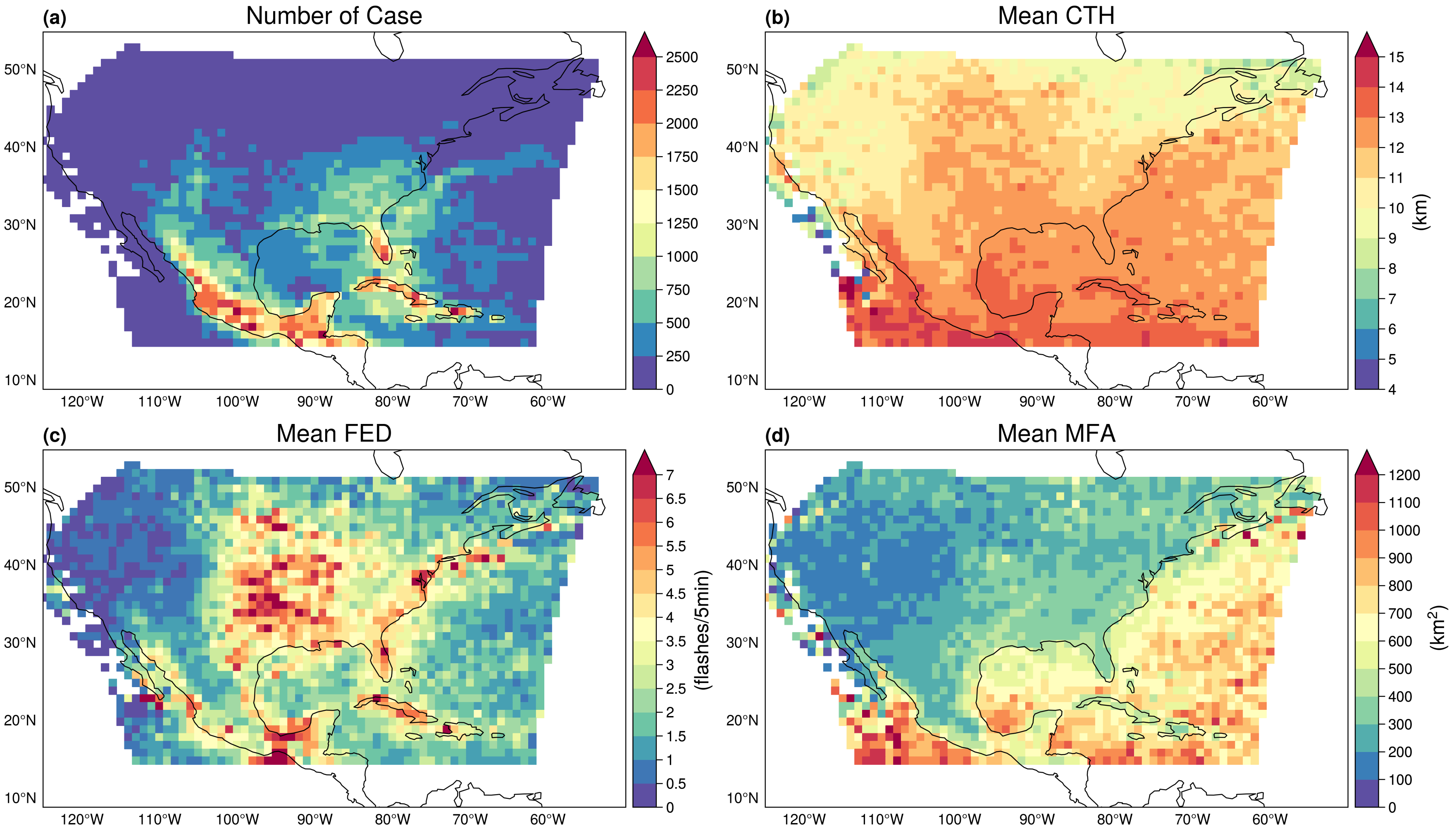
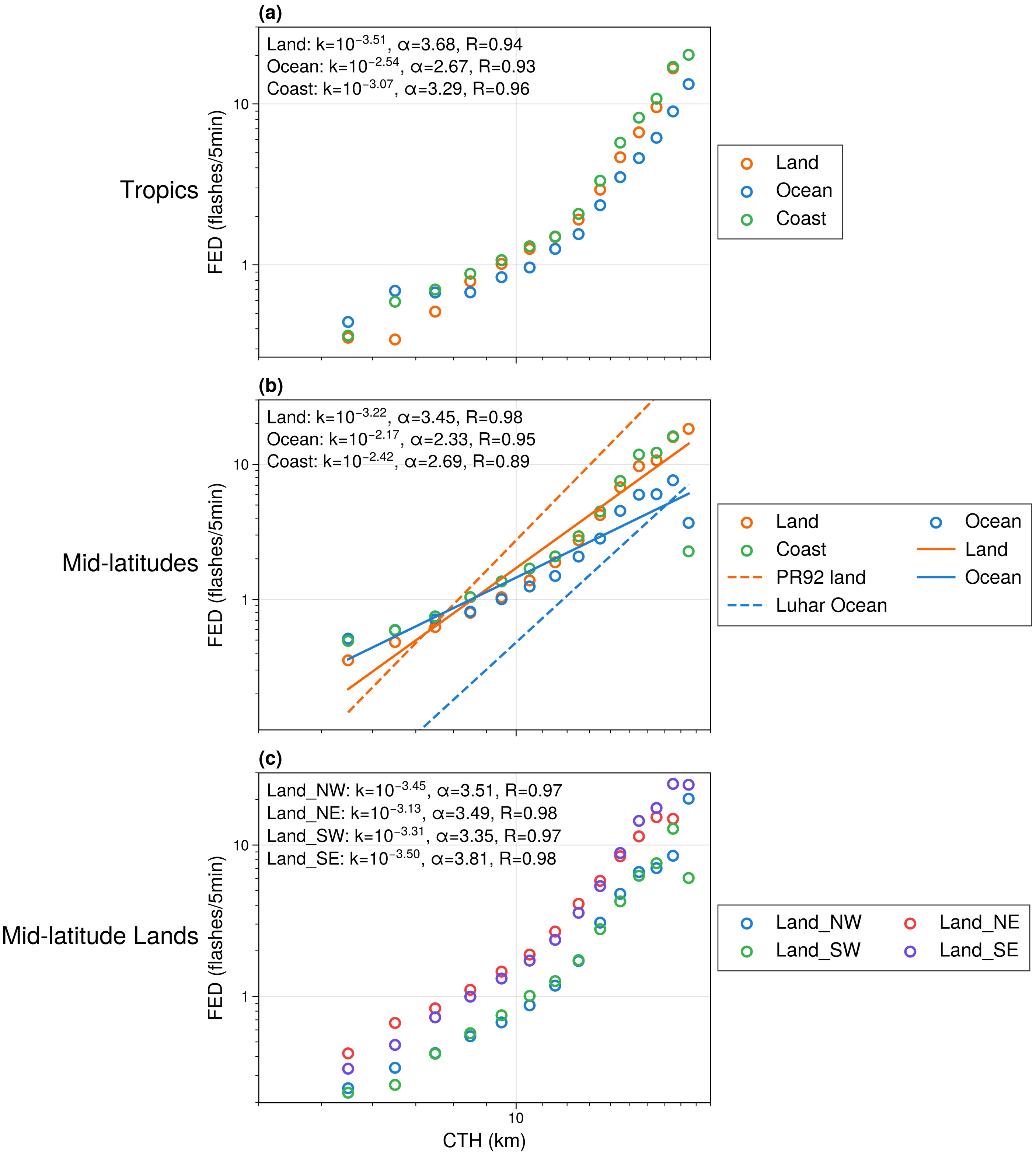
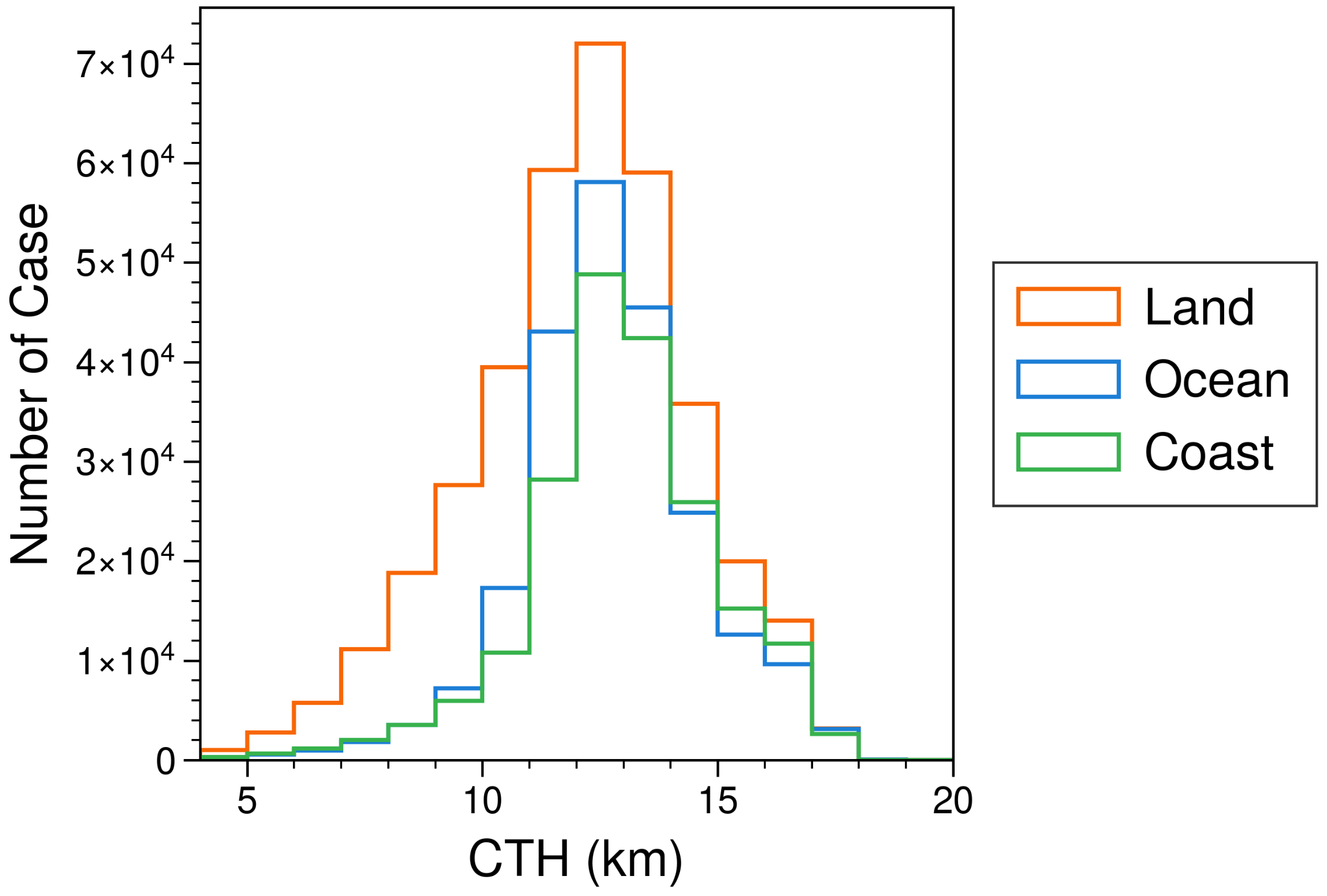
3.1. Regional Variations
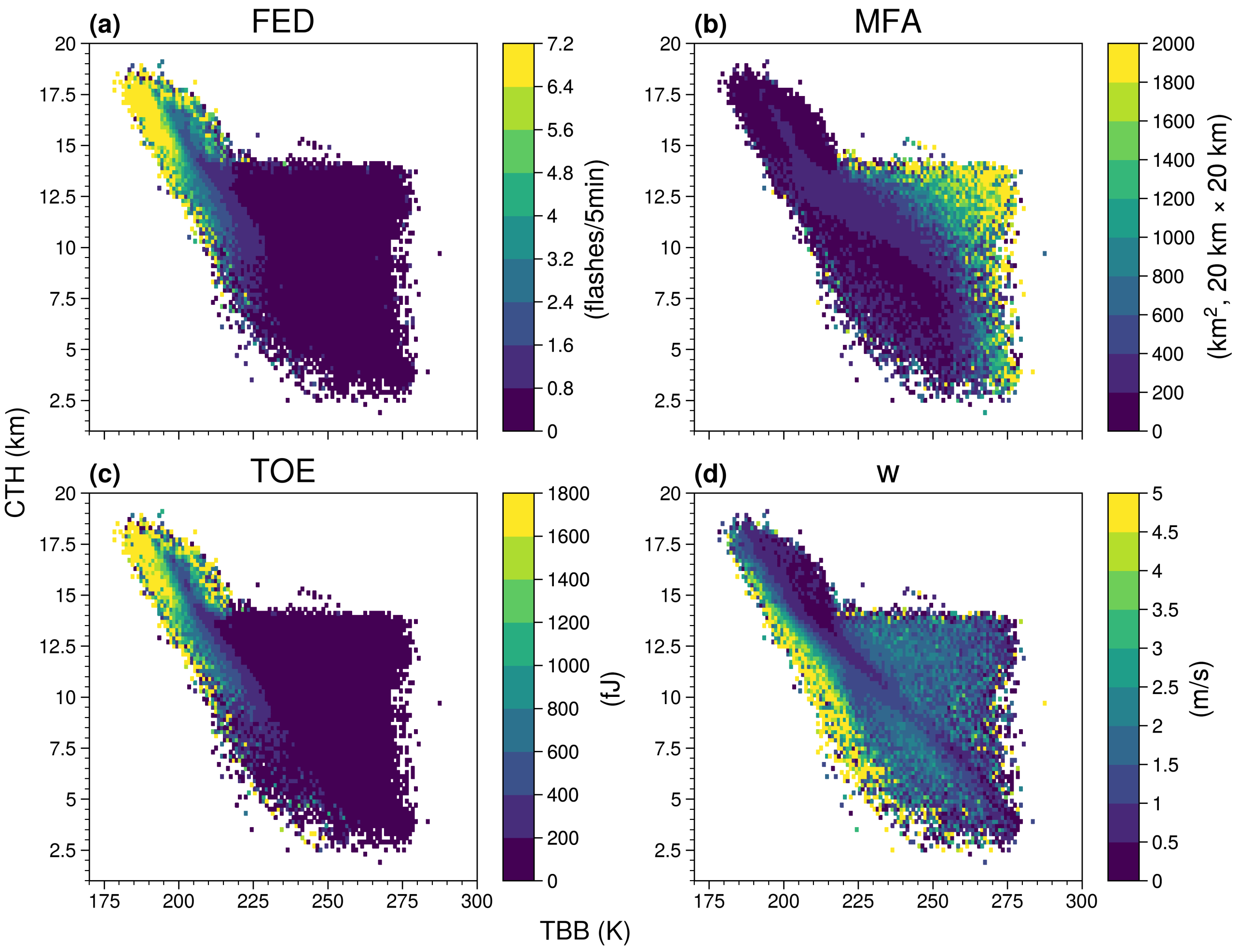
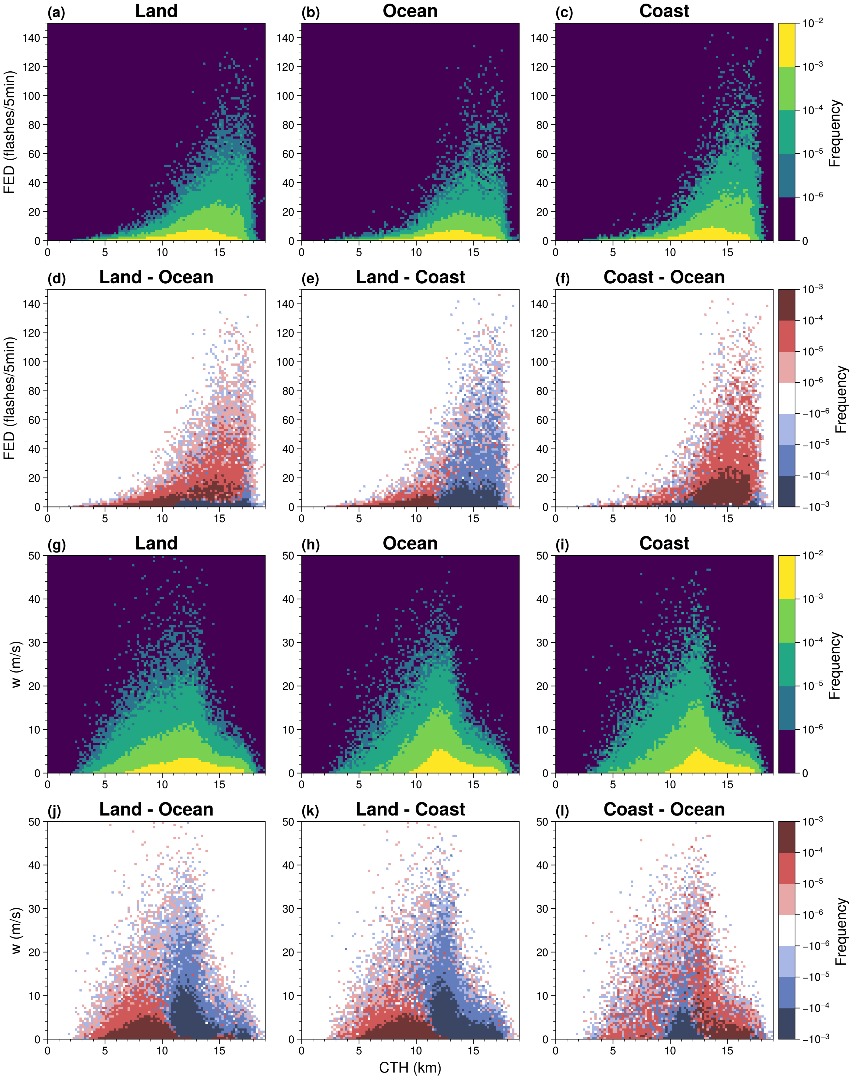
3.2. ABI-GLM Relationships
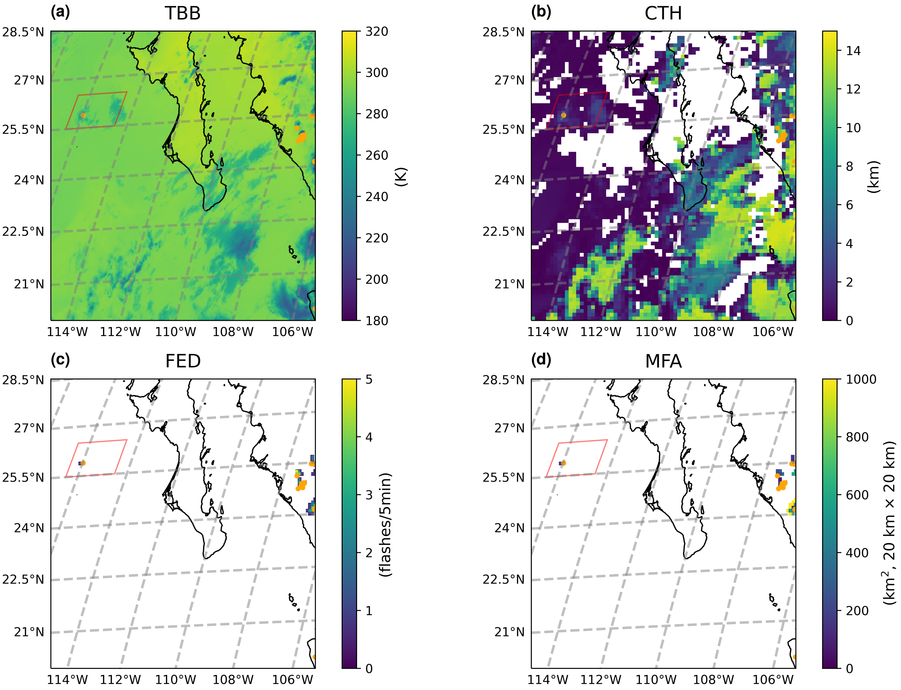
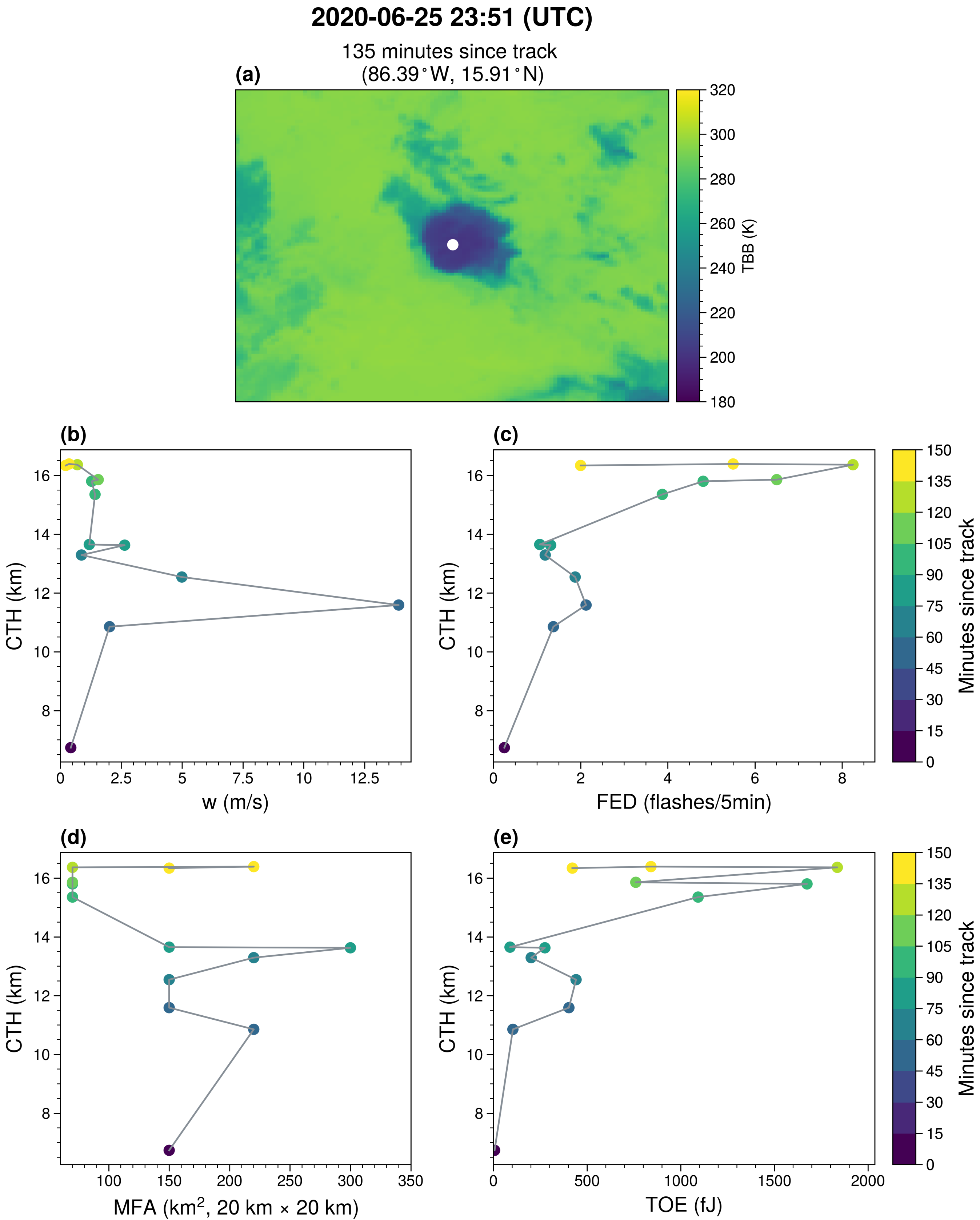
3.3. Case Studies
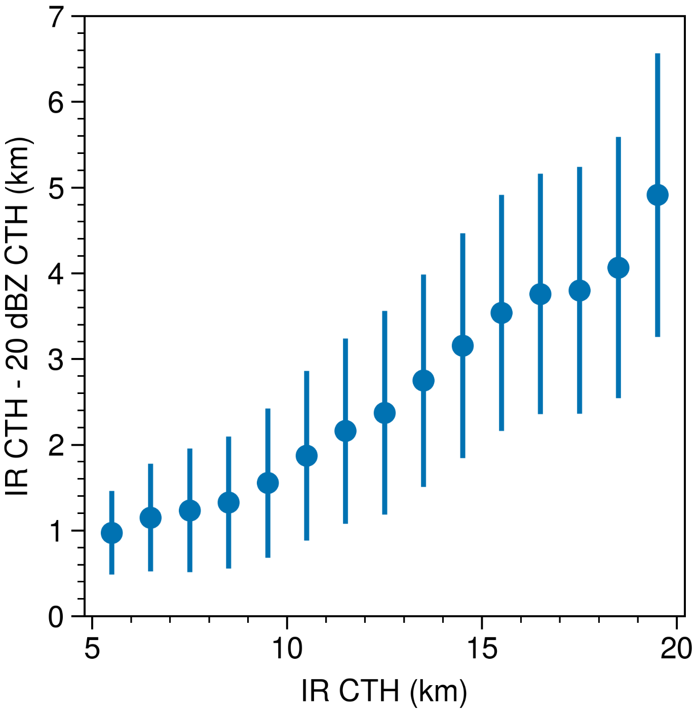
3.4. CTH Proxy
4. Conclusions
Author Contributions
Funding
Institutional Review Board Statement
Informed Consent Statement
Data Availability Statement
Acknowledgments
Conflicts of Interest
References
- Blakeslee, R.J.; Lang, T.J.; Koshak, W.J.; Buechler, D.; Gatlin, P.; Mach, D.M.; Stano, G.T.; Virts, K.S.; Walker, T.D.; Cecil, D.J.; et al. Three Years of the Lightning Imaging Sensor Onboard the International Space Station: Expanded Global Coverage and Enhanced Applications. J. Geophys. Res. Atmos. 2020, 125, e2020JD032918. [Google Scholar] [CrossRef]
- Aich, V.; Holzworth, R.; Goodman, S.; Kuleshov, Y.; Price, C.; Williams, E. Lightning: A New Essential Climate Variable. Eos 2018, 99. [Google Scholar] [CrossRef]
- Price, C. Will a Drier Climate Result in More Lightning? Atmos. Res. 2009, 91, 479–484. [Google Scholar] [CrossRef]
- Price, C.; Yair, Y.; Mugnai, A.; Lagouvardos, K.; Llasat, M.; Michaelides, S.; Dayan, U.; Dietrich, S.; Galanti, E.; Garrote, L.; et al. The FLASH Project: Using Lightning Data to Better Understand and Predict Flash Floods. Environ. Sci. Policy 2011, 14, 898–911. [Google Scholar] [CrossRef] [Green Version]
- Harel, M.; Price, C. Thunderstorm Trends over Africa. J. Clim. 2020, 33, 2741–2755. [Google Scholar] [CrossRef]
- Etten-Bohm, M.; Yang, J.; Schumacher, C.; Jun, M. Evaluating the Relationship Between Lightning and the Large-Scale Environment and Its Use for Lightning Prediction in Global Climate Models. J. Geophys. Res. Atmos. 2021, 126, e2020JD033990. [Google Scholar] [CrossRef]
- Yair, Y. Lightning Hazards to Human Societies in a Changing Climate. Environ. Res. Lett. 2018, 13, 123002. [Google Scholar] [CrossRef]
- Schumann, U.; Huntrieser, H. The Global Lightning-Induced Nitrogen Oxides Source. Atmos. Chem. Phys. 2007, 7, 3823–3907. [Google Scholar] [CrossRef] [Green Version]
- Pickering, K.E.; Thompson, A.M.; Tao, W.K.; Kucsera, T.L. Upper Tropospheric Ozone Production Following Mesoscale Convection during STEP/EMEX. J. Geophys. Res. Atmos. 1993, 98, 8737–8749. [Google Scholar] [CrossRef]
- Morris, G.A.; Thompson, A.M.; Pickering, K.E.; Chen, S.; Bucsela, E.J.; Kucera, P.A. Observations of Ozone Production in a Dissipating Tropical Convective Cell during TC4. Atmos. Chem. Phys. 2010, 10, 11189–11208. [Google Scholar] [CrossRef] [Green Version]
- Huntrieser, H.; Lichtenstern, M.; Scheibe, M.; Aufmhoff, H.; Schlager, H.; Pucik, T.; Minikin, A.; Weinzierl, B.; Heimerl, K.; Fütterer, D.; et al. On the Origin of Pronounced O3 Gradients in the Thunderstorm Outflow Region during DC3. J. Geophys. Res. Atmos. 2016, 121, 6600–6637. [Google Scholar] [CrossRef] [Green Version]
- Myhre, G.; Shindell, D.; Bréon, F.M.; Collins, W.; Fuglestvedt, J.; Huang, J.; Koch, D.; Lamarque, J.F.; Lee, D.; Mendoza, B. Climate Change 2013: The Physical Science Basis. Contribution of Working Group I to the Fifth Assessment Report of the Intergovernmental Panel on Climate Change; Tignor, M.K., Allen, S.K., Boschung, J., Nauels, A., Xia, Y., Bex, V., Midgley, P.M., Eds.; Cambridge University Press: Cambridge, UK; New York, NY, USA, 2013. [Google Scholar]
- Molinie, G.; Jacobson, A.R. Cloud-to-Ground Lightning and Cloud Top Brightness Temperature over the Contiguous United States. J. Geophys. Res. Atmos. 2004, 109. [Google Scholar] [CrossRef]
- Thiel, K.C.; Calhoun, K.M.; Reinhart, A.E.; MacGorman, D.R. GLM and ABI Characteristics of Severe and Convective Storms. J. Geophys. Res. Atmos. 2020, 125, e2020JD032858. [Google Scholar] [CrossRef]
- Tessendorf, S.A.; Miller, L.J.; Wiens, K.C.; Rutledge, S.A. The 29 June 2000 Supercell Observed during STEPS. Part I: Kinematics and Microphysics. J. Atmos. Sci. 2005, 62, 4127–4150. [Google Scholar] [CrossRef]
- Deierling, W.; Petersen, W.A. Total Lightning Activity as an Indicator of Updraft Characteristics. J. Geophys. Res. Atmos. 2008, 113. [Google Scholar] [CrossRef] [Green Version]
- Romps, D.M.; Seeley, J.T.; Vollaro, D.; Molinari, J. Projected Increase in Lightning Strikes in the United States Due to Global Warming. Science 2014, 346, 851–854. [Google Scholar] [CrossRef]
- Finney, D.L.; Doherty, R.M.; Wild, O.; Stevenson, D.S.; MacKenzie, I.A.; Blyth, A.M. A Projected Decrease in Lightning under Climate Change. Nat. Clim. Chang. 2018, 8, 210–213. [Google Scholar] [CrossRef]
- Romps, D.M. Evaluating the Future of Lightning in Cloud-resolving Models. Geophys. Res. Lett. 2019, 46, 14863–14871. [Google Scholar] [CrossRef]
- Hudman, R.C.; Jacob, D.J.; Turquety, S.; Leibensperger, E.M.; Murray, L.T.; Wu, S.; Gilliland, A.B.; Avery, M.; Bertram, T.H.; Brune, W.; et al. Surface and Lightning Sources of Nitrogen Oxides over the United States: Magnitudes, Chemical Evolution, and Outflow. J. Geophys. Res. Atmos. 2007, 112. [Google Scholar] [CrossRef] [Green Version]
- Gressent, A.; Sauvage, B.; Cariolle, D.; Evans, M.; Leriche, M.; Mari, C.; Thouret, V. Modeling Lightning-NOx Chemistry on a Sub-Grid Scale in a Global Chemical Transport Model. Atmos. Chem. Phys. 2016, 16, 5867–5889. [Google Scholar] [CrossRef] [Green Version]
- Price, C.; Rind, D. A Simple Lightning Parameterization for Calculating Global Lightning Distributions. J. Geophys. Res. Atmos. 1992, 97, 9919–9933. [Google Scholar] [CrossRef]
- Vonnegut, B. Some Facts and Speculations Concerning the Origin and Role of Thunderstorm Electricity. In Severe Local Storms; Atlas, D., Booker, D.R., Byers, H., Douglas, R.H., Fujita, T., House, D.C., Ludlum, F.H., Malkus, J.S., Newton, C.W., Ogura, Y., et al., Eds.; American Meteorological Society: Boston, MA, USA, 1963; pp. 224–241. [Google Scholar] [CrossRef]
- Williams, E.R. Large-Scale Charge Separation in Thunderclouds. J. Geophys. Res. Atmos. 1985, 90, 6013. [Google Scholar] [CrossRef]
- Clark, S.K.; Ward, D.S.; Mahowald, N.M. Parameterization-Based Uncertainty in Future Lightning Flash Density. Geophys. Res. Lett. 2017, 44, 2893–2901. [Google Scholar] [CrossRef]
- Luhar, A.K.; Galbally, I.E.; Woodhouse, M.T.; Abraham, N.L. Assessing and Improving Cloud-Height-Based Parameterisations of Global Lightning Flash Rate, and Their Impact on Lightning-Produced NOx and Tropospheric Composition in a Chemistry–Climate Model. Atmos. Chem. Phys. 2021, 21, 7053–7082. [Google Scholar] [CrossRef]
- Boccippio, D.J. Lightning Scaling Relations Revisited. J. Atmos. Sci. 2002, 59, 1086–1104. [Google Scholar] [CrossRef]
- Ushio, T.; Heckman, S.J.; Boccippio, D.J.; Christian, H.J.; Kawasaki, Z.I. A Survey of Thunderstorm Flash Rates Compared to Cloud Top Height Using TRMM Satellite Data. J. Geophys. Res. Atmos. 2001, 106, 24089–24095. [Google Scholar] [CrossRef]
- Futyan, J.M.; Genio, A.D.D. Relationships between Lightning and Properties of Convective Cloud Clusters. Geophys. Res. Lett. 2007, 34. [Google Scholar] [CrossRef] [Green Version]
- Sieglaff, J.M.; Cronce, L.M.; Feltz, W.F.; Bedka, K.M.; Pavolonis, M.J.; Heidinger, A.K. Nowcasting Convective Storm Initiation Using Satellite-Based Box-Averaged Cloud-Top Cooling and Cloud-Type Trends. J. Appl. Meteor. Climatol. 2011, 50, 110–126. [Google Scholar] [CrossRef]
- Adler, R.F.; Fenn, D.D. Thunderstorm Vertical Velocities Estimated from Satellite Data. J. Atmos. Sci. 1979, 36, 1747–1754. [Google Scholar] [CrossRef] [Green Version]
- Hamada, A.; Takayabu, Y.N. Convective Cloud Top Vertical Velocity Estimated from Geostationary Satellite Rapid-Scan Measurements. Geophys. Res. Lett. 2016, 43, 5435–5441. [Google Scholar] [CrossRef] [Green Version]
- Yang, J.; Zhang, Z.; Wei, C.; Lu, F.; Guo, Q. Introducing the New Generation of Chinese Geostationary Weather Satellites, Fengyun-4. Bull. Amer. Meteor. Soc. 2017, 98, 1637–1658. [Google Scholar] [CrossRef]
- Hui, W.; Zhang, W.; Lyu, W.; Li, P. Preliminary Observations from the China Fengyun-4A Lightning Mapping Imager and Its Optical Radiation Characteristics. Remote Sens. 2020, 12, 2622. [Google Scholar] [CrossRef]
- Rudlosky, S.D.; Goodman, S.J.; Virts, K.S.; Bruning, E.C. Initial Geostationary Lightning Mapper Observations. Geophys. Res. Lett. 2019, 46, 1097–1104. [Google Scholar] [CrossRef]
- Cao, D.; Lu, F.; Zhang, X.; Yang, J. Lightning Activity Observed by the FengYun-4A Lightning Mapping Imager. Remote Sens. 2021, 13, 3013. [Google Scholar] [CrossRef]
- Orville, R.E.; Henderson, R.W. Absolute Spectral Irradiance Measurements of Lightning from 375 to 880 Nm. J. Atmos. Sci. 1984, 41, 3180–3187. [Google Scholar] [CrossRef] [Green Version]
- Goodman, S.J.; Christian, H.J.; Rust, W.D. A Comparison of the Optical Pulse Characteristics of Intracloud and Cloud-to-Ground Lightning as Observed above Clouds. J. Appl. Meteor. 1988, 27, 1369–1381. [Google Scholar] [CrossRef] [Green Version]
- Goodman, S.J.; Blakeslee, R.J.; Koshak, W.J.; Mach, D.; Bailey, J.; Buechler, D.; Carey, L.; Schultz, C.; Bateman, M.; McCaul, E., Jr.; et al. The GOES-R Geostationary Lightning Mapper (GLM). Atmos. Res. 2013, 125-126, 34–49. [Google Scholar] [CrossRef] [Green Version]
- Edgington, S.; Tillier, C.; Anderson, M. Design, Calibration, and on-Orbit Testing of the Geostationary Lightning Mapper on the GOES-R Series Weather Satellite. In Proceedings of the International Conference on Space Optics—ICSO, Chania, Greece, 9–12 October 2018; Karafolas, N., Sodnik, Z., Cugny, B., Eds.; SPIE: Chania, Greece, 2019; p. 143. [Google Scholar] [CrossRef] [Green Version]
- Mach, D.M. Geostationary Lightning Mapper Clustering Algorithm Stability. J. Geophys. Res. Atmos. 2020, 125, e2019JD031900. [Google Scholar] [CrossRef]
- Mach, D.M.; Christian, H.J.; Blakeslee, R.J.; Boccippio, D.J.; Goodman, S.J.; Boeck, W.L. Performance Assessment of the Optical Transient Detector and Lightning Imaging Sensor. J. Geophys. Res. Atmos. 2007, 112, D09210. [Google Scholar] [CrossRef]
- Christian, H.; Blakeslee, R.; Goodman, S.; Mach, D. Algorithm Theoretical Basis Document (ATBD) for the Lightning Imaging Sensor (LIS); NASA/Marshall Space Flight Center: Huntsville, AL, USA, 2000; 53p. [Google Scholar]
- Goodman, S.; Mach, D.; Koshak, W.; Blakeslee, R. Algorithm Theoretical Basis Document (ATBD) for the GLM Lightning Cluster-Filter Algorithm; NESDIS Center for Satellite Applications and Research v2.0; NOAA: Washington, DC, USA, 2010. [Google Scholar]
- Bateman, M.; Mach, D.; Stock, M. Further Investigation into Detection Efficiency & False Alarm Rate for the Geostationary Lightning Mappers aboard GOES-16 and GOES-17. Earth. Space. Sci. 2020, 8, e2020EA001237. [Google Scholar] [CrossRef]
- Rodger, C.J.; Brundell, J.B.; Dowden, R.L.; Thomson, N.R. Location Accuracy of Long Distance VLF Lightning Locationnetwork. Ann. Geophys. 2004, 22, 747–758. [Google Scholar] [CrossRef] [Green Version]
- Liu, C.; Sloop, C.; Heckman, S. Application of Lightning in Predicting High Impact Weather. In Proceedings of the WMO Technical Conference on Meteorological and Environmental Instruments and Methods of Observation, Saint Petersburg, Russia, 7 July 2014; Volume 9. [Google Scholar]
- Cummins, K.L.; Murphy, M.J. An Overview of Lightning Locating Systems: History, Techniques, and Data Uses, with an In-Depth Look at the U.S. NLDN. IEEE Trans. Electromagn. Compat. 2009, 51, 499–518. [Google Scholar] [CrossRef]
- Murphy, M.J.; Said, R.K. Comparisons of Lightning Rates and Properties from the U.S. National Lightning Detection Network (NLDN) and GLD360 With GOES-16 Geostationary Lightning Mapper and Advanced Baseline Imager Data. J. Geophys. Res. Atmos. 2020, 125, e2019JD031172. [Google Scholar] [CrossRef]
- Bruning, E.C.; Tillier, C.E.; Edgington, S.F.; Rudlosky, S.D.; Zajic, J.; Gravelle, C.; Foster, M.; Calhoun, K.M.; Campbell, P.A.; Stano, G.T.; et al. Meteorological Imagery for the Geostationary Lightning Mapper. J. Geophys. Res. Atmos. 2019, 124, 14285–14309. [Google Scholar] [CrossRef]
- Bruning, E. Deeplycloudy/Glmtools: Glmtools Release to Accompany Publication. Zenodo 2019. [Google Scholar] [CrossRef]
- Calhoun, K.M.; MacGorman, D.R.; Ziegler, C.L.; Biggerstaff, M.I. Evolution of Lightning Activity and Storm Charge Relative to Dual-Doppler Analysis of a High-Precipitation Supercell Storm. Mon. Wea. Rev. 2013, 141, 2199–2223. [Google Scholar] [CrossRef]
- Mecikalski, R.M.; Bain, A.L.; Carey, L.D. Radar and Lightning Observations of Deep Moist Convection across Northern Alabama during DC3: 21 May 2012. Mon. Wea. Rev. 2015, 143, 2774–2794. [Google Scholar] [CrossRef]
- Rudlosky, S.D.; Goodman, S.J.; Virts, K.S. Lightning Detection: GOES-R Series Geostationary Lightning Mapper. In The GOES-R Series; Elsevier: Amsterdam, The Netherlands, 2020; pp. 193–202. [Google Scholar] [CrossRef]
- Hersbach, H.; Bell, B.; Berrisford, P.; Hirahara, S.; Horányi, A.; Muñoz-Sabater, J.; Nicolas, J.; Peubey, C.; Radu, R.; Schepers, D.; et al. The ERA5 Global Reanalysis. Q. J. R. Meteorol. Soc. 2020, 146, 1999–2049. [Google Scholar] [CrossRef]
- Heikenfeld, M.; Marinescu, P.J.; Christensen, M.; Watson-Parris, D.; Senf, F.; van den Heever, S.C.; Stier, P. Tobac 1.2: Towards a Flexible Framework for Tracking and Analysis of Clouds in Diverse Datasets. Geosci. Model Dev. 2019, 12, 4551–4570. [Google Scholar] [CrossRef] [Green Version]
- Soille, P.J.; Ansoult, M.M. Automated Basin Delineation from Digital Elevation Models Using Mathematical Morphology. Signal Process. 1990, 20, 171–182. [Google Scholar] [CrossRef]
- Allan, D.B.; Caswell, T.; Keim, N.C.; van der Wel, C.M.; Verweij, R.W. Soft-Matter/Trackpy: Trackpy v0.5.0. Zenodo, 2021. [Google Scholar] [CrossRef]
- Kelso, N.V. Nvkelso/Natural-Earth-Vector. 2021. Available online: https://www.naturalearthdata.com/downloads/ (accessed on 27 September 2021).
- Christian, H.J.; Blakeslee, R.J.; Boccippio, D.J.; Boeck, W.L.; Buechler, D.E.; Driscoll, K.T.; Goodman, S.J.; Hall, J.M.; Koshak, W.J.; Mach, D.M.; et al. Global Frequency and Distribution of Lightning as Observed from Space by the Optical Transient Detector. J. Geophys. Res. Atmos. 2003, 108, ACL-4-1–ACL-4-15. [Google Scholar] [CrossRef]
- Ramesh Kumar, P.; Kamra, A.K. Land–Sea Contrast in Lightning Activity over the Sea and Peninsular Regions of South/Southeast Asia. Atmos. Res. 2012, 118, 52–67. [Google Scholar] [CrossRef]
- Kaplan, J.O.; Lau, K.H.K. The WGLC Global Gridded Lightning Climatology and Time Series. Earth Syst. Sci. Data 2021, 13, 3219–3237. [Google Scholar] [CrossRef]
- Peterson, M.; Mach, D.; Buechler, D. A Global LIS/OTD Climatology of Lightning Flash Extent Density. J. Geophys. Res. Atmos. 2021, 126, e2020JD033885. [Google Scholar] [CrossRef]
- Zipser, E.J.; Lutz, K.R. The Vertical Profile of Radar Reflectivity of Convective Cells: A Strong Indicator of Storm Intensity and Lightning Probability? Mon. Wea. Rev. 1994, 122, 1751–1759. [Google Scholar] [CrossRef] [Green Version]
- Bang, S.D.; Zipser, E.J. Differences in Size Spectra of Electrified Storms over Land and Ocean. Geophys. Res. Lett. 2015, 42, 6844–6851. [Google Scholar] [CrossRef]
- Aumann, H.H.; DeSouza-Machado, S.G.; Behrangi, A. Deep Convective Clouds at the Tropopause. Atmos. Chem. Phys. 2011, 11, 1167–1176. [Google Scholar] [CrossRef] [Green Version]
- Boccippio, D.J.; Cummins, K.L.; Christian, H.J.; Goodman, S.J. Combined Satellite- and Surface-Based Estimation of the Intracloud–Cloud-to-Ground Lightning Ratio over the Continental United States. Mon. Weather Rev. 2001, 129, 108–122. [Google Scholar] [CrossRef]
- Yoshida, S.; Morimoto, T.; Ushio, T.; Kawasaki, Z. A Fifth-Power Relationship for Lightning Activity from Tropical Rainfall Measuring Mission Satellite Observations. J. Geophys. Res. Atmos. 2009, 114. [Google Scholar] [CrossRef]
- Liu, C.Y.; Chiu, C.H.; Lin, P.H.; Min, M. Comparison of Cloud-Top Property Retrievals From Advanced Himawari Imager, MODIS, CloudSat/CPR, CALIPSO/CALIOP, and Radiosonde. J. Geophys. Res. Atmos. 2020, 125, e2020JD032683. [Google Scholar] [CrossRef]
- Jeyaratnam, J.; Luo, Z.J.; Giangrande, S.E.; Wang, D.; Masunaga, H. A Satellite-Based Estimate of Convective Vertical Velocity and Convective Mass Flux: Global Survey and Comparison With Radar Wind Profiler Observations. Geophys. Res. Lett. 2021, 48, e2020GL090675. [Google Scholar] [CrossRef]
- Williams, E.; Stanfill, S. The Physical Origin of the Land–Ocean Contrast in Lightning Activity. Comptes Rendus Physique 2002, 3, 1277–1292. [Google Scholar] [CrossRef]
- Takahashi, T. Riming Electrification as a Charge Generation Mechanism in Thunderstorms. J. Atmos. Sci. 1978, 35, 1536–1548. [Google Scholar] [CrossRef]
- Zipser, E.J.; LeMone, M.A. Cumulonimbus Vertical Velocity Events in GATE. Part II: Synthesis and Model Core Structure. J. Atmos. Sci. 1980, 37, 2458–2469. [Google Scholar] [CrossRef] [Green Version]
- Romps, D.M.; Charn, A.B. Sticky Thermals: Evidence for a Dominant Balance between Buoyancy and Drag in Cloud Updrafts. J. Atmos. Sci. 2015, 72, 2890–2901. [Google Scholar] [CrossRef]
- Liu, C.; Zipser, E.J.; Nesbitt, S.W. Global Distribution of Tropical Deep Convection: Different Perspectives from TRMM Infrared and Radar Data. J. Climate 2007, 20, 489–503. [Google Scholar] [CrossRef]
- Song, H.J.; Kim, S.; Roh, S.; Lee, H. Difference Between Cloud Top Height and Storm Height for Heavy Rainfall Using TRMM Measurements. J. Meteorol. Soc. 2020, 98, 901–914. [Google Scholar] [CrossRef]
- Peterson, M.; Rudlosky, S.; Zhang, D. Changes to the Appearance of Optical Lightning Flashes Observed From Space According to Thunderstorm Organization and Structure. J. Geophys. Res. Atmos. 2020, 125, e2019JD031087. [Google Scholar] [CrossRef] [PubMed]
- Marchand, M.; Hilburn, K.; Miller, S.D. Geostationary Lightning Mapper and Earth Networks Lightning Detection Over the Contiguous United States and Dependence on Flash Characteristics. J. Geophys. Res. Atmos. 2019, 124, 11552–11567. [Google Scholar] [CrossRef]
- Liu, C.; Zipser, E.J.; Cecil, D.J.; Nesbitt, S.W.; Sherwood, S. A Cloud and Precipitation Feature Database from Nine Years of TRMM Observations. J. Appl. Meteor. Climatol. 2008, 47, 2712–2728. [Google Scholar] [CrossRef]
- Bateman, M.; Mach, D. Preliminary Detection Efficiency and False Alarm Rate Assessment of the Geostationary Lightning Mapper on the GOES-16 Satellite. J. Appl. Remote. Sens. 2020, 14, 032406. [Google Scholar] [CrossRef]
- Holmlund, K.; Grandell, J.; Schmetz, J.; Stuhlmann, R.; Bojkov, B.; Munro, R.; Lekouara, M.; Coppens, D.; Viticchie, B.; August, T.; et al. Meteosat Third Generation (MTG): Continuation and Innovation of Observations from Geostationary Orbit. Bull. Amer. Meteor. Soc. 2021, 102, E990–E1015. [Google Scholar] [CrossRef]
- Zhang, X. Xin_RS_2021_GOES_lightning_data. Zenodo, 2021. [Google Scholar] [CrossRef]
- Zhang, X. Zxdawn/Xin_RS_2021_GOES_lightning: Version 1.0. Zenodo, 2021. [Google Scholar] [CrossRef]
- Davis, L.L.B. ProPlot. Zenodo, 2021. [Google Scholar] [CrossRef]
- Raspaud, M.; Hoese, D.; Dybbroe, A.; Lahtinen, P.; Devasthale, A.; Itkin, M.; Hamann, U.; Rasmussen, L.Ø.; Neilsen, E.S.; Leppelt, T.; et al. PyTroll: An Open-Source, Community-Driven Python Framework to Process Earth Observation Satellite Data. Bull. Amer. Meteor. Soc. 2018, 99, 1329–1336. [Google Scholar] [CrossRef] [Green Version]
- Raspaud, M.; Hoese, D.; Lahtinen, P.; Finkensieper, S.; Holl, G.; Dybbroe, A.; Proud, S.; Meraner, A.; Zhang, X.; Joro, S.; et al. Pytroll/Satpy: Version 0.25.1. Zenodo 2021. [Google Scholar] [CrossRef]


| Area | Region * | Number of Tracked Pixels |
|---|---|---|
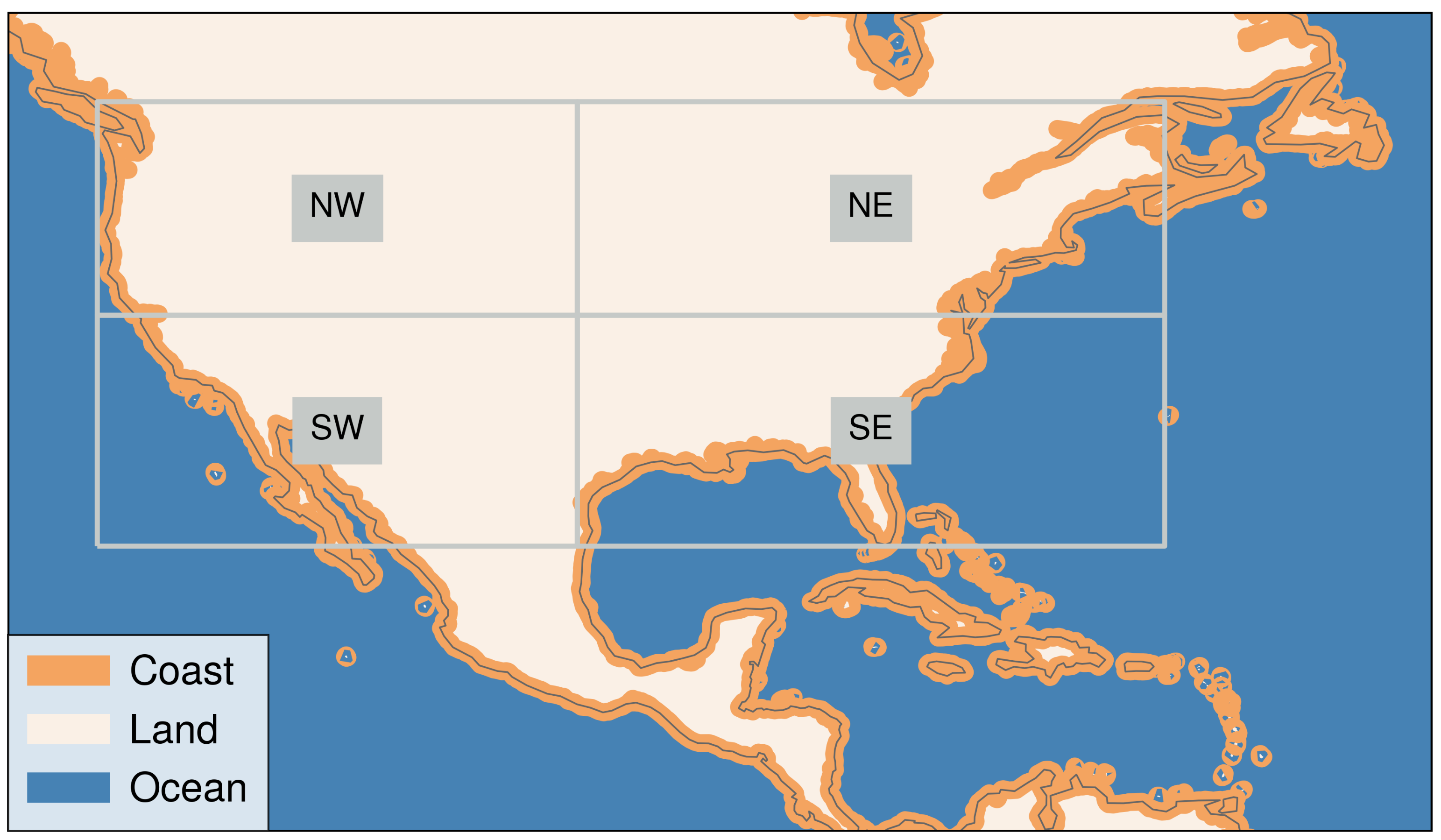
| Land | NW (38–50 N, 98–125 W) | 27,273 |
| NE (38–50 N, 65–98 W) | 48,378 | |
| SW (25–38 N, 98–125 W) | 75,156 | |
| SE (25–38 N, 65–98 W) | 77,091 | |
| Tropics (<23.5 N) | 123,409 | |
| Mid-latitudes (≥23.5 N) | 246,765 | |
| CONUS (GOES-16 scan) | 370,174 | |
| Ocean | Tropics (<23.5 N) | 96,773 |
| Mid-latitudes (≥23.5 N) | 132,013 | |
| CONUS (GOES-16 scan) | 228,786 | |
| Coast | Tropics (<23.5 N) | 134,719 |
| Mid-latitudes (≥23.5 N) | 64,797 | |
| CONUS (GOES-16 scan) | 199,516 |
Publisher’s Note: MDPI stays neutral with regard to jurisdictional claims in published maps and institutional affiliations. |
© 2021 by the authors. Licensee MDPI, Basel, Switzerland. This article is an open access article distributed under the terms and conditions of the Creative Commons Attribution (CC BY) license (https://creativecommons.org/licenses/by/4.0/).
Share and Cite
Zhang, X.; Yin, Y.; Kukulies, J.; Li, Y.; Kuang, X.; He, C.; Lapierre, J.L.; Jiang, D.; Chen, J. Revisiting Lightning Activity and Parameterization Using Geostationary Satellite Observations. Remote Sens. 2021, 13, 3866. https://0-doi-org.brum.beds.ac.uk/10.3390/rs13193866
Zhang X, Yin Y, Kukulies J, Li Y, Kuang X, He C, Lapierre JL, Jiang D, Chen J. Revisiting Lightning Activity and Parameterization Using Geostationary Satellite Observations. Remote Sensing. 2021; 13(19):3866. https://0-doi-org.brum.beds.ac.uk/10.3390/rs13193866
Chicago/Turabian StyleZhang, Xin, Yan Yin, Julia Kukulies, Yang Li, Xiang Kuang, Chuan He, Jeff L. Lapierre, Dongxin Jiang, and Jinghua Chen. 2021. "Revisiting Lightning Activity and Parameterization Using Geostationary Satellite Observations" Remote Sensing 13, no. 19: 3866. https://0-doi-org.brum.beds.ac.uk/10.3390/rs13193866