1. Introduction
Gravity observations are a well-established element of today’s Earth observation from space. Measurement of the gravity field reveals Earth’s state of mass balance and its dynamics and provides the geoid as reference for sea level, global ocean circulation and height systems, and the variations of gravity and of the geoid provide information on mass exchange processes in the Earth system [
1].
The GOCE satellite [
2] was orbiting from 2009 to 2013 at a mean altitude of 255 km (nominal mission) and 225 km (extended mission) in drag-free mode. The scientific payload was a gravity gradiometer, which consisted of six ultraprecise accelerometers, and a dual-frequency GPS receiver. The measurements of these instruments were used to derive gravity gradients and precise orbits, which were transformed into a gravity map of Earth with a mean global accuracy of 2 cm in terms of geoid heights and 0.5 mGal for gravity anomalies, at 100 km spatial resolution [
3]. The low controlled altitude, the drag compensation control (so-called “drag-free”) and the accurate angular accelerations measured as a by-product of the gradiometer payload were all instrumental in GOCE’s outstanding result.
From 2002 to 2017, the GRACE satellites [
4] provided measurements that were processed to obtain monthly estimates of Earth’s global gravity field at scales of several hundreds of kilometers and larger. The time variations of the gravity field were used to determine changes in Earth’s mass distribution [
5], with applications ranging from measurement of continental water storage (e.g., seasonal changes in large river basins and groundwater depletion) [
6,
7,
8,
9,
10], to ice and snow accumulation and depletion in the polar regions and large glaciers [
11,
12,
13], to the monitoring of global mean barystatic sea-level variations and oceans [
14,
15,
16,
17,
18,
19,
20]. The two GRACE satellites were identical and flew in near-circular, polar (89° inclination) orbits, initially at 500 km altitude, at along-track distance varying around a mean value of 220 km. The instantaneous distance variation measured by a dual-band microwave ranging instrument (24 GHz, 32 GHz) was the main observable, supplemented by GPS positions and nongravitational acceleration measured by high-precision accelerometers. The satellite altitude decayed naturally under atmospheric drag down to about 320 km at the end of the extended mission lifetime, with the consequence that the ground track pattern was changing continuously, resulting in variable quality of monthly solutions.
The GRACE Follow-On (GRACE-FO) satellites [
21] were launched on 22 May 2018 and are meant to continue the GRACE time series for at least five years. The satellite design is fully inherited from GRACE but includes a laser ranging interferometer (LRI) as a technology demonstration of a more precise ranging capability.
Acceleration measurement errors (e.g., temperature-induced bias drifts), the relatively high and variable altitude and the one-dimensional North–South sampling are known to affect the GRACE gravity model quality. Improvements to the spacecraft design (thermal control, attitude measurement and control) can help to reduce systematic errors. Beyond that, however, aliasing mainly due to monthly temporal sampling dominates due to unavoidable errors in the aliasing reduction modeling of high-frequency ocean and atmospheric mass variations: even a substantially improved instrument such as the LRI cannot be fully exploited [
22]. A single pair of satellites cannot meet operational and global user community needs. This would result only in partial information, and it would not be possible to support key applications, e.g., ground water and aquifer monitoring for improved water management, at the required spatiotemporal resolution. A future gravity mission dedicated to mass change in the Earth system, as studied in the context of a Next Generation Gravity Mission [
23], will require improvements in the instrumentation, the spacecraft (disturbing accelerations) and the mission design (sampling). In addition, a constellation of two pairs of satellites in an optimized orbit configuration and a strategy for reducing potential remaining aliasing errors are required.
A number of authors have studied future gravity field mission concepts based on precise ranging between two low-flying satellites forming a pair. Most of them considered either a single pair flying in formation or two satellite pairs flying in a so-called Bender constellation [
24], where one pair is in a polar orbit and the other pair in an orbit with an inclination of 63° (see, e.g., [
25] and the references therein). Other satellite formations, such as the Cartwheel, Pendulum and Helix formations, impose excessive attitude and orbit control and, consequently, power demands on the satellite system and were therefore abandoned. The favored option seems to be the Bender constellation with two satellite pairs flying in an in-line formation like the GRACE and GRACE-FO satellites.
The orbit optimization of the Bender constellation is a complex problem. For individual satellite pairs, we could use the Nyquist-type rule introduced in [
26] or its revised version presented in [
27]. For a Bender constellation, [
28] proposed to use a genetic algorithm. All these approaches have the drawback that they optimize the orbits for a single temporal resolution, whereas multiple temporal resolutions are required to serve the needs of all users [
28,
29]. For this reason, a new orbit selection approach that aims at optimizing the spatial sampling of the Bender constellation for multiple temporal resolutions [
30] was developed. The approach was successfully used for generating the orbits in a number of ESA-funded simulation studies [
31,
32,
33].
NGGM can be understood as one of the Bender pairs of the MAGIC constellation, providing either global coverage via the polar pair or enhanced coverage of the mid-latitudes through the inclined pair. In this case, the combination of NGGM with a second pair is under study together with NASA to arrive at the MAGIC constellation. The global user community requirements were identified by the Joint NASA/ESA Ad-hoc Science Study Team (AJSST) composed of US and European representatives of the global scientific community, for a univocal consolidation of the threshold and target user requirements and initial mission requirements for observation systems orbiting at different altitudes. The Mission Requirements Document (MRD) includes user and application needs in user community reports from the IUGG [
29], the NASA/ESA Interagency Gravity Science Working Group [
34], the US Decadal Survey for Earth Science and Applications from Space [
35] and other recent work cited in the MRD. A full science traceability matrix can be found in
Appendix A of the MRD [
36].
The spatiotemporal mapping shall be such that atmospheric, ocean and ocean tide (AO + OT) signals and/or errors can be decoupled from signals from other Earth system constituents (ice, hydrology, oceans and solid Earth), taking into account possible aliasing periods. Notably, a double satellite pair mission concept has the intrinsic potential to retrieve the full atmosphere, ocean, hydrology, ice and solid Earth (AOHIS) signal in contrast to a single-pair mission, where tailored postprocessing further reduces the signal and is not able to achieve the same resolution and performance as a double-pair mission without postprocessing [
31].
Following the orbit optimization problems, the methodology to derive the engineering system requirements is presented: the paper also addresses the mission-enabling technology (i.e., propulsion) and corresponding instrument performances, the accelerometer selection for the selected set of orbits and the drag compensation solution and its versatility in order to address the entwined impact of different levels of drag compensation designs and related orbit altitudes on the mission performance.
2. Orbit Selection Approach
The satellites’ altitude is a key parameter for spatial and temporal sampling. A drag compensation system can also maintain the altitude and offers the opportunity to select it such that the spatial and temporal sampling is optimal for the gravity field retrieval. This is an important difference with respect to the GRACE and GRACE-FO missions, where the orbits were allowed to drift naturally and, consequently, the satellites slowly decayed over time due to atmospheric drag. Here, we describe an approach for the selection of orbits of two satellite pairs flying in a Bender constellation [
24], where one pair is placed in a polar orbit and the other one in an inclined orbit with an approximate inclination of 70°. This approach was used to define constellations that were investigated in the recent mission simulation studies [
31,
32] funded by ESA and also analyzed together with JPL in [
37].
To serve the needs of the broad range of users of time-variable gravity field models [
29], our objective is to optimize the constellation’s spatial sampling for the recovery of mass change signals in a range of temporal scales. The orbit selection is therefore closely related to the characteristics of the mass change signals in space and time, which are realistically represented in the Earth system model (ESM) [
38,
39]. These characteristics are illustrated in
Figure 1, which shows the amplitude spectral density (ASD) of the combined nontidal mass change signals in the atmosphere, oceans, land hydrology, land cryosphere and solid Earth. The ASD was calculated for each spherical harmonic coefficient of the time-variable gravitational potential using Welch’s method [
40] and then averaged per degree.
Figure 1 shows large day-to-day mass change signals, which originate to a large extent from the atmosphere and oceans [
39]. Since the daily spatial sampling is a consequence of the period of the orbiting satellite and of the fact that Earth makes one full rotation per day, densifying the daily spatial sampling can only be achieved with more satellite pairs. In the gravity field model retrieval, one may use the Wiese approach [
41] or the daily Kalman filter method [
42] for the (co)estimation of daily gravity field models. Mass change signals with a period of a few days are significantly smaller than the day-to-day ones. In a sense, it takes a few days before the accumulated mass change signal is large enough to become appreciable and, thus, worthwhile to account for in a gravity field model. In contrast to the one-day period, it is, however, possible to optimize a constellation for the retrieval of gravity field models spanning a few days. Simulations by [
32] demonstrated that the Bender constellation in combination with a certain accuracy level of the instruments allows the estimation of 3-day gravity field models, even though the spatial sampling is sparse due to the limited number of orbital revolutions within that period. For periods longer than three days, the amplitude of the mass change signals and the number of orbital revolutions increase further. Hence, it is expected that it will be much less challenging to find a constellation that offers a sufficiently dense spatial sampling for the retrieval of, e.g., monthly gravity field models, and capturing the time-variable signal within the month at shorter intervals will also improve monthly models.
Since we aim for optimizing the spatial sampling at multiple temporal resolutions (daily to weekly, monthly to seasonal and long-term trends), we need a tool to assess the spatial sampling as a function of time and altitude, where the latter is the parameter that we select in the optimization process. In the following, we introduce two graphs for that purpose: the first graph will guide the selection of the altitudes of the individual satellite pairs, and the second is used for fine-tuning of the selected altitudes, such that the interleaving of the ground tracks of the two satellite pairs remains fixed for one of the temporal resolutions.
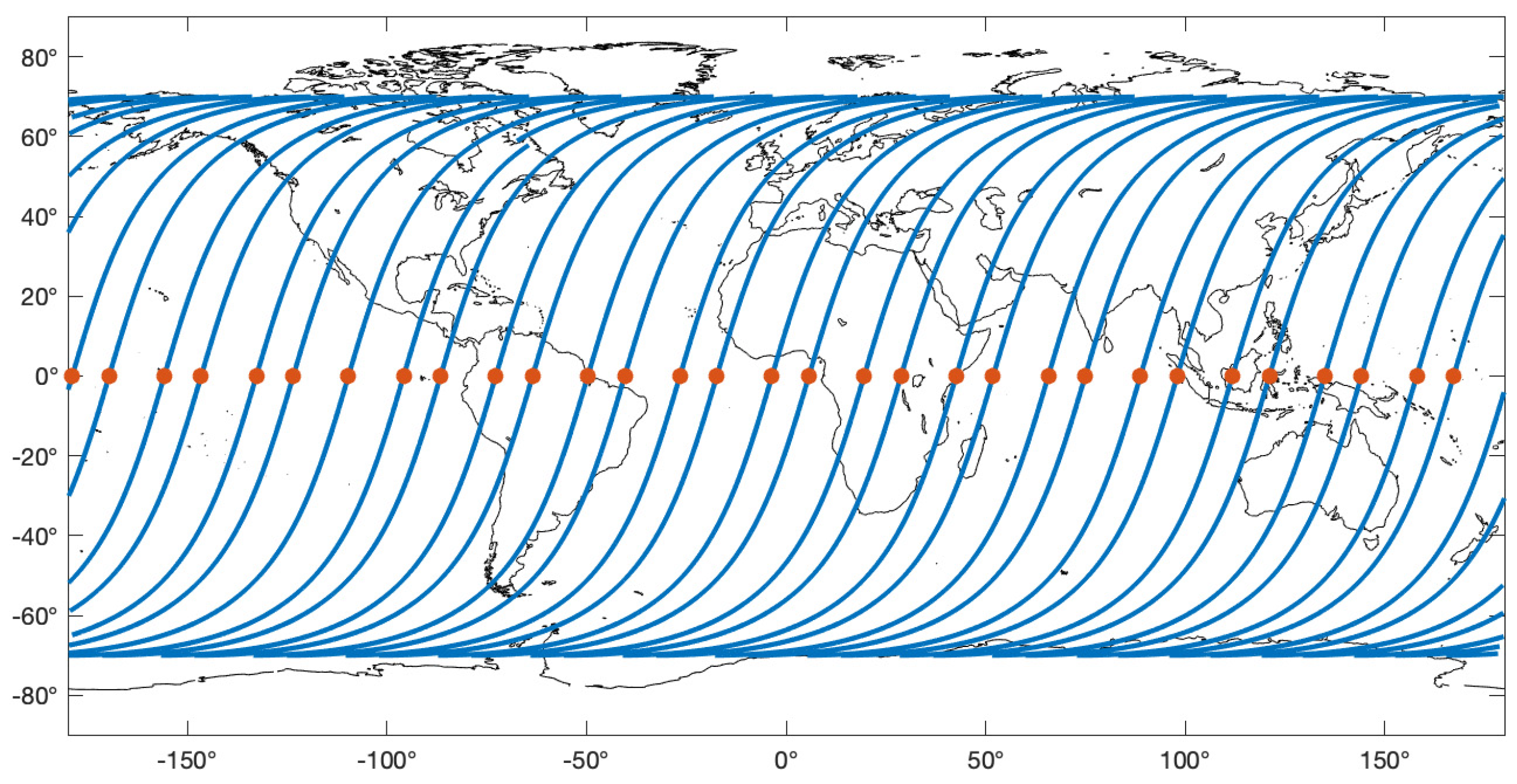
Generally, the satellites for measuring the gravity field need to orbit as low as possible because the magnitude of the gravity field is stronger at lower altitudes. To spend as much time as possible at low altitudes, circular orbits are preferred. To enable the retrieval of gravity field models with a high resolution in space and time, we need to achieve a dense spatial sampling with a minimum number of orbital revolutions. To analyze the denseness of the sampling, we exploit the fact that the ground tracks of two arbitrary revolutions of a circular orbit differ mainly in longitude at the equator. We simplify by considering only the ascending tracks, i.e., the half of the ground track where the satellite is orbiting northward. Obviously, the spatial sampling is as dense as possible when the intersections of the ascending tracks at the Earth equator are evenly distributed along the equator. This is illustrated in
Figure 2, which shows 31 ascending tracks of a circular orbit with a semimajor axis of 6,718,085 m and an inclination of 70°. The intersections of the ascending tracks and the equator, to which we refer as ascending equator crossings in the following, are marked by red dots. Since they are almost evenly distributed, the spatial sampling is near homogeneous; i.e., it is almost as dense as possible for that number of orbital revolutions.
To quantify the denseness of the spatial sampling at a predefined number of orbital revolutions, we define the ground track homogeneity
.
is the ratio of the largest and the smallest difference between adjacent ascending equator crossings, denoted by and, respectively, where is the number of orbital revolutions. The value indicates that the ground track repeats every orbital revolutions, which is the definition of a repeat orbit. Values larger than unity, but still close to unity, indicate near-repeat orbits. In the following, we describe how to calculate the homogeneity .
We start with the difference in longitude between one ascending equator crossing and another after
orbital revolutions,
where
is the secular motion of the ascending node,
is Earth’s mean angular velocity and
is the orbital period. The secular motion of the ascending node is defined as
where
is Earth’s gravitational constant,
is Earth’s dynamical form factor,
R is the equatorial radius of the Earth (6.3781366 × 10
6 m), is the semimajor axis of the orbit,
is the eccentricity of the orbit and
is the inclination of the orbit. The orbital period is
which remains practically constant as an orbit maintenance and/or drag compensation system can ensure the spacecraft’s target altitude.
Let
denote the longitude of the
th ascending equator crossing, which we may freely select. Then, the longitudes of all other ascending equator crossings can be calculated by
Alternatively, we could determine the longitudes of the ascending equator crossings through orbit integration. Successively, we sort the first
longitudes in ascending order, so that they form a monotonously increasing sequence.
The largest and the smallest difference of the cyclic sequence of sorted longitudes are
and
respectively. Since we are interested in the denseness of the spatial sampling, we calculate these differences for
orbital revolutions to find when the largest difference in longitude is notably reduced, i.e., when the spatial sampling densifies. Both differences are bounded by
, which is the lower bound for
and the upper bound for
.
Figure 3 illustrates the differences and the bounding value of
for the first 90 orbital revolutions of the circular orbit presented in
Figure 2. The differences typically remain constant for a number of orbital revolutions before they are notably reduced, i.e., they depart from the bounding value of
and then make a step back towards that value. To find such steps, we check when the largest difference in longitude is reduced from one orbital revolution to the next one, more than its lower bound; i.e., we search for the index
, for which
The differences that fulfill Equation (9) are marked by black circles in
Figure 3. We calculate the ground track homogeneity only for these differences, which we signified by using the same index
in Equations (1) and (9). In this way, we identify at which numbers of orbital revolutions the ground track is near homogeneous, i.e., when we achieve a dense spatial sampling with a minimum number of orbital revolutions.
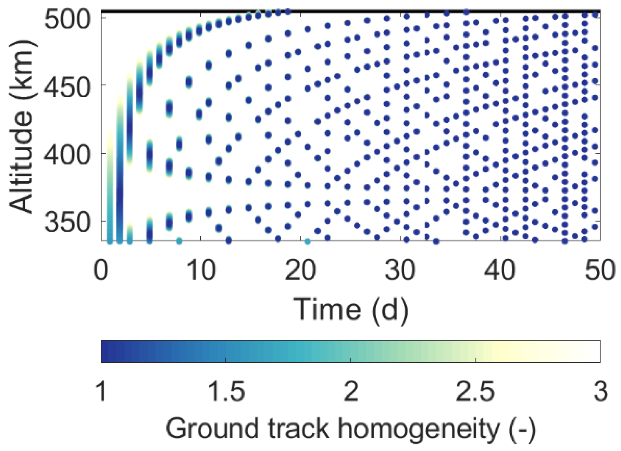
Since the altitude is the parameter to optimize, we calculate the homogeneity for a large number of orbits whose orbital elements are identical except for the semimajor axis. In practice, we repeat the calculations for all values of the semimajor axis in the range from
to
in steps of
. While the range is typically predefined, we need to select the step size
. For that purpose, we determine how much the longitude of the last ascending equator crossing,
, changes when the semimajor axis is altered by
. This change in longitude, denoted by
, can be derived from the differential of Equation (2)
where
and
We select the step size
such that the longitude of the last ascending equator crossing changes at most by
which is the smallest possible reduction of
from the second-last to the last orbital revolution. In this way, we found the step size
for semimajor axes in the range of 6718–6888 km, which corresponds to an altitude range of 340–510 km, and
(50 days). On the left,
Figure 4 presents all homogeneity values
in that altitude range within a time span of 1–50 days. This graph is particularly useful for selecting the altitude of the individual satellite pairs of the constellation. We only have to draw a horizontal line into the graph to identify whether an altitude provides small homogeneity values, i.e., a dense spatial sampling, for the desired time spans and obtain an overview of the achievable subcycles offered by the selected altitude.
Generally, the graph in
Figure 4 reveals that for shorter time spans small homogeneity values stretch over much larger altitude ranges than for longer time spans. At three days, for example, homogeneity values
stretch from 406 to 433 km, i.e., over an altitude range of 27 km. This altitude range offers many other small homogeneity values at longer time spans, which gives flexibility for optimizing the spatial sampling at multiple temporal resolutions. We propose using this flexibility to optimize the constellation in the following way: First, we note that the ground track will shift by
after
orbital revolutions.
Figure 5 shows
for the homogeneity values
, which are illustrated in
Figure 4. For homogeneity values equal to 1, which correspond to repeat orbits, the ground track shift is obviously zero. Generally, homogeneity values close to 1 result in small ground track shifts.
The first step of the constellation optimization is the selection of the shortest period that is longer than one day and shall be resolved by the gravity field modeling. Since the spatial sampling is obviously less dense for shorter time spans, we select altitudes of the satellite pairs such that both their ground tracks exhibit the same within that short period. Then, the crossover points of the satellite pairs’ ground tracks will shift in longitude by after orbital revolutions, whereas their latitude will not change. In a sense, the interleaving of these ground tracks for a single pair of satellites will nearly repeat every orbital revolutions, such that the density of the spatial sampling within that short period does not change over time. This feature ensures a constant quality of gravity field models for each chosen estimation period, which is an important benefit for emergency and operational applications and services.
Since we only require that
is the same for both satellite pairs, we still have the flexibility to select the altitudes such that the orbits offer near-homogeneity values at longer periods. In practice, we create plots of the homogeneity and ground track shift as shown in
Figure 4 and
Figure 5 for both satellite pairs. Then, we search for the altitudes that offer near-homogeneity values for a number of periods, which relate to the desired temporal resolutions (for example, 1 week and 1 month), and fulfill the constraint that the ground track shift of the shortest period longer than one day is the same for both satellite pairs. Thus, the combination of the two plots as illustrated in
Figure 4 and
Figure 5 enables us to optimize the sampling of each individual pair as well as the constellation. The latter optimization can be achieved by interleaving the sampling of the second pair at the equator in between the sampling of the first one, resulting in an effective doubling of the spatial resolution, which can be achieved for a given period.
As mentioned before, the orbits used in several ESA studies were selected by the approach described in this section. For example, [
31] based their simulations on orbits with inclinations of 70 and 89° and altitudes of 355 and 340 km, respectively, and a ground track shift of 1.3° every 7 days. In addition to the period of 7 days, the orbit with an inclination of 70° offered a near-homogeneity value of 1.1 at 19 days, whereas the orbit with an inclination of 89° offered a near-homogeneity value of 1.1 at 18 days. Thus, the sampling was optimized for the retrieval of weekly as well as 18–19-day gravity field models.
3. Application to the MAGIC Mission
The approach described in the previous section was used to identify a starting set of orbits for the Phase A studies of the NGGM mission concept. Achieving accurate and purely satellite-based solutions on daily to weekly time scales is not possible with the current generation of gravity missions. MAGIC aims at responding to this objective to improve current models and in particular to introduce the capability to support monitoring and mitigating extreme events. For this reason, particular attention was paid to weekly/subweekly subcycles in the MAGIC orbit candidates’ selection process. Another benefit of the choice of these near-homogeneous short periods is that, for example, weekly variations within each month are separable from the monthly variations, thus resulting in improved monthly solutions.
The so-called Bender constellation consisting of two satellite pairs flying at two different orbit inclinations was identified as the most promising concept to meet the global user community requirements and is currently the baseline for MAGIC. This constellation type is favored over other formations due to its good performance for the gravity field retrieval and its implementation options allowing different spatial resolution results to be obtained for different periods. As stated in version 1 of the Mission Requirements Document (MRD) [
36], the constellation shall consist of two pairs: the first one in a near-polar orbit and the second one with an inclination between 65 and 70°. A deviation from these inclinations, such as up to 75°, can be investigated if another orbit sampling/coverage is favorable for specific applications. In addition, the mission shall provide a near-homogeneous sampling over a subcycle of 3–7 days. To quantify the density of the spatial sampling at a predefined number of orbital revolutions, we can use the ground track homogeneity parameter (
). In order to select the optimal orbits for the two pairs, it is necessary to search for the altitudes that offer small homogeneity values for a number of periods common to both, which relate to the desired temporal resolutions and fulfill the constraint of the same ground track shift for both pairs at the targeted subweekly subcycle. Thus, the combination of the homogeneity and ground track shift in longitude and the interleaving of the sampling of both pairs at the equator enables optimized sampling of the individual pairs as well as the constellation.
In this section, we discuss the orbit candidates for a polar pair (PP) and an inclined pair (IP), which we have identified using the method introduced in
Section 2. The orbits are assumed to be at a constant mean altitude over the mission lifetime and the solutions are optimized for 5- and 7-day subcycles. Beyond this subweekly sampling, the presented scenarios offer at least another subcycle between 28 and 32 days, which guarantees for monthly solutions a near-homogeneous ground track as well. The ground track homogeneity is considered to range between 1.0 and 1.5 as a goal and 1.5 and 2.0 as a threshold. Since shorter periods have a lower ground track density than longer periods for the same value of
, the subweekly samplings are selected with a more rigid constraint of
< 1.5.
A large number of inclinations are introduced to illustrate the sampling capabilities. Inclined pairs are studied for inclinations of 65, 67, 70 and 75°, while polar pairs are investigated for 87, 88 and 89°. For the polar pair, a high inclination is preferred to avoid polar gaps. However, in this initial phase, lower inclinations (e.g., 87 and 88°) were also introduced to provide a broader range of sampling options for the two pairs.
3.1. Five-Day Subcycle
Table 1 lists near-optimal orbits for the 5-day subcycle sampling for the inclined and polar pair. In order to create a good constellation encompassing the inclined and polar pair, it is necessary as a first approximate step to choose between the different listed cases, selecting the combinations with minimal difference in longitude shift. When doing so, for each targeted subcycle, the two pairs could have an overlapping ground track crossing at the equator, or, probably better, interleaved tracks filling in gaps from the first pair by the second pair.
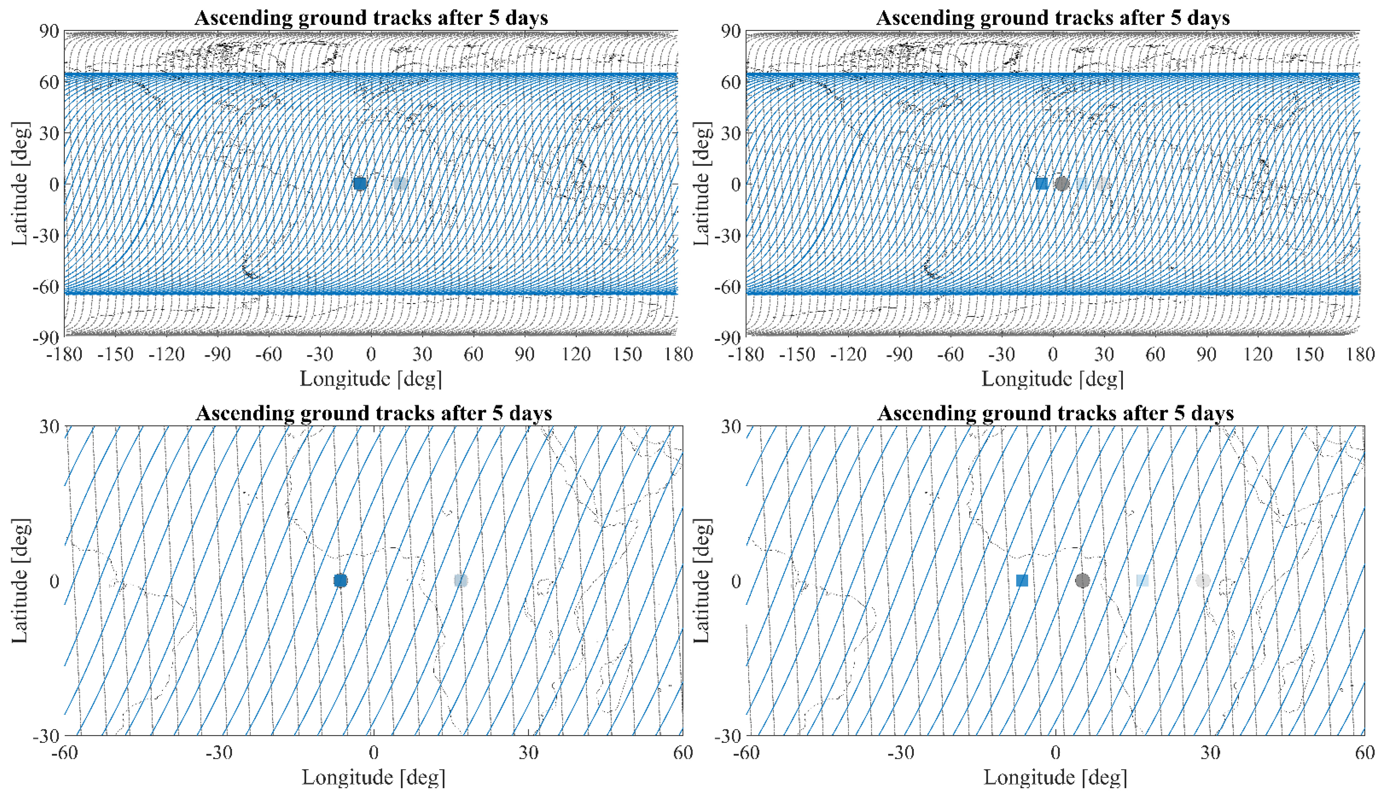
Figure 6 illustrates an example of the ground tracks after 5 days for one of the optimized scenarios listed above. In particular, this figure shows the accumulated ascending ground tracks in 5 days for an inclined pair at 396 km and 65° of inclination and a polar pair at 434 km and 89°. In this example, the orbits are chosen in order to have an overlap of the ground track position of the satellites (inclined and polar pairs) at the ascending node (on the left in
Figure 6) or to have interleaved positions at the equator to enhance the spatial sampling (on the right in
Figure 6). Ground track near homogeneity for the two altitudes and inclinations is shown in
Figure 7.
3.2. Seven-Day Subcycle
Table 2 lists the near-optimal orbits of the inclined and polar pair for the 7-day subcycle sampling. As it can be observed, the number of possibilities is reduced with respect to the 5-day scenario. This is due to the ground track homogeneities, which are more sensitive to changes in altitude for longer subcycles. The latter can also be seen from
Figure 4, where the altitude ranges, over which small homogeneity values stretch, appears reciprocal to the length of the subcycles.
3.3. Recommended Orbits
Based on previous
Table 1 and
Table 2, it is possible to identify specific sets of orbits that are nearly nullifying the difference in the ground track longitude shifts for certain subweekly subcycles (
Table 3). The inclinations and/or altitudes in
Table 3 can be fine-tuned to make sure that the longitude shifts of the two pairs have an exact match. For example, in the worst case of scenario 3d_M, it would require a + 0.2° change in inclination or a 321 m change in altitude for the inclined pair. See
Appendix B for the full table of matching combinations. The 5- and 7-day subcycle scenarios are identified by “5d” and “7d”, respectively. The scenario ID is supplemented by “M” for medium and “H” for higher altitudes. These IDs are associated with having one or two sets at altitudes approximately between 400 and 450 km and over 450 km, respectively. Altitudes over 500 km are not recommended due to the too low sensitivity to the gravity signal and to the limit in achieving the user needs as shown in the
Appendix B of the MAGIC MRD [
36]. For completeness, two scenarios optimized for 3 days are also introduced in the following table to provide additional options, should higher priority be given to short time scales for example for near-real-time applications. As additional information, the last column of
Table 3 provides a list of all the common subcycles achievable by both pairs. As previously mentioned, all the recommended scenarios include at least one subcycle between 28 and 32 days. As discussed before, higher importance is given to the homogeneity at short time scales. A more detailed version of
Table 3 is provided in
Appendix A.
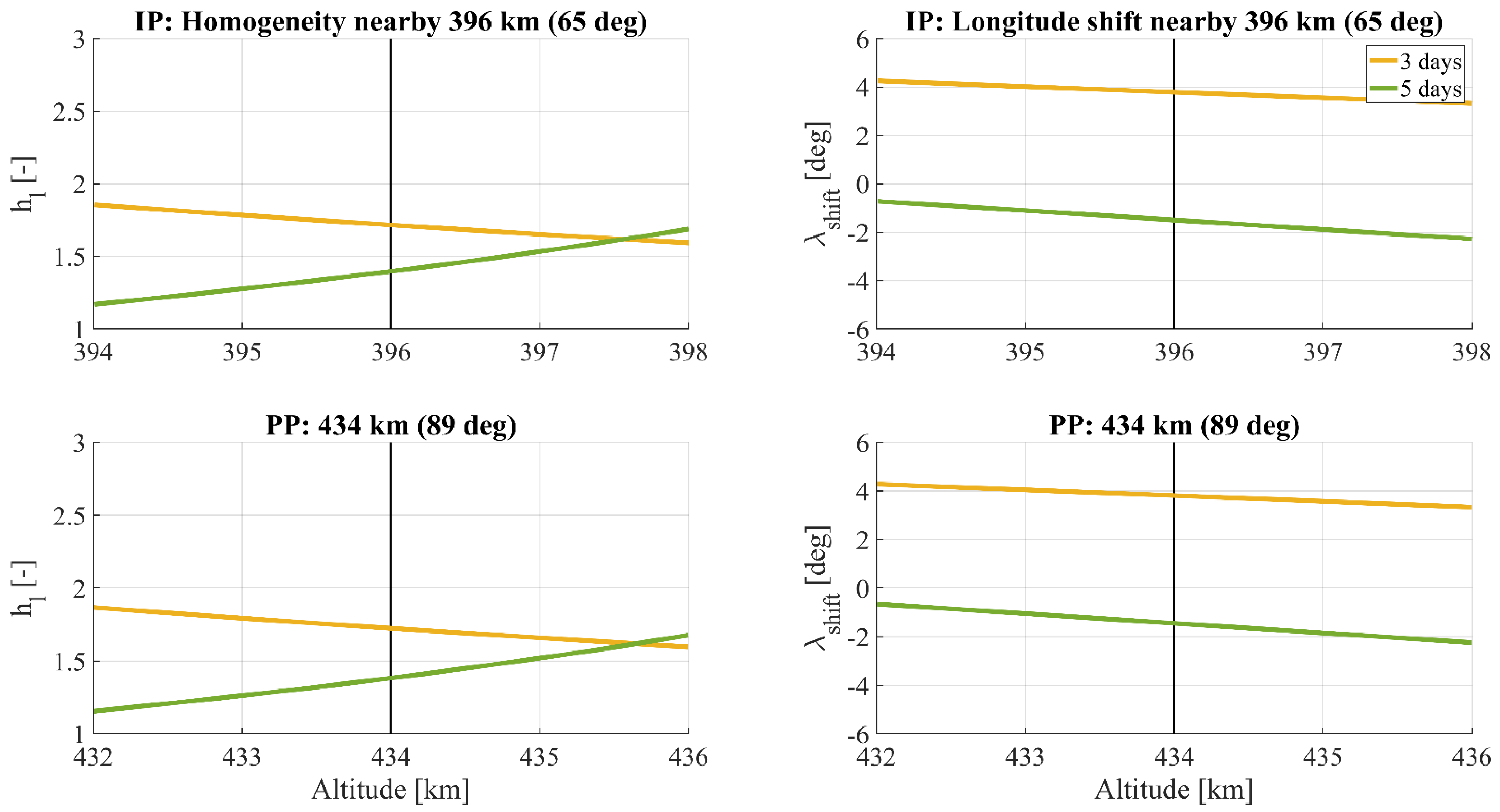
Figure 8 illustrates the sensitivity to altitude changes (±2 km) around the altitudes of the 5d_Ma orbit candidate, while
Table 4 quantifies the variations for
hl and longitude shifts for all the recommended orbits. The change in homogeneity and longitude shift of the 3-day subcycles can be around 2 and 5 times less sensitive to a change in altitude than the 5- and 7-day examples, respectively.
The values are estimated at the scenarios’ altitudes, and the ones between brackets are for subcycles with 2< hl <3. The consequences of the altitude variation are given to provide relevant information for the system design and further scientific studies.
The orbit inclination is a less strict parameter and nearly does not change over the mission lifetime. However, if a change in inclination would be required, it is important to know that inclination changes of ±1° for subcycles of 3, 5 and 7 days can modify the ground track homogeneity with an average 0.07, 0.15 and 0.26 deg−1, respectively. This further confirms the higher stability of 3-day solutions and the low influence of the inclination changes on the homogeneity also for longer subcycles.
4. Instrument Sensitivity, Accelerometer and Drag Compensation Assessment
The aim of NGGM as part of the MAGIC constellation is to obtain relatively high-resolution measurements in space and time, including the capability to determine and separate the contributions in the variations of the gravity field due to mass change in terrestrial water storage (i.e., for hydrology thematic field), cryosphere, oceans, solid Earth and climate change signals. This capability enables the mission to serve science and operational applications, including services. The user requirements in [
29,
34] have been established based on an exhaustive list of mass change signals for each of the thematic fields of interest listed above and are expressed as cumulative equivalent water height (EWH) error thresholds/goals per spherical harmonic (SH) degree of expansion of the Earth gravity field model. Such requirements form the basis for deriving observation requirements.
We describe here a tool that helps in trading off between technical feasibility and fulfilling user requirements for the accuracy and spatiotemporal resolution of the gravity field solutions taking into account the heritage from previous missions and engineering knowledge of specific technology to be embarked on the satellites. Thus, the scope is to search for the acceptable noise level of the ranging and acceleration observations in dependence on altitude and intersatellite distance. These two mission parameters have an unavoidable impact on the mission design and performance: a lower altitude implies a (multiaxis) drag compensation, and a larger intersatellite distance reduces the impact of accelerometer noise but changes the sensitivity to small-scale gravity signals.
The search space for the space segment design is rather vast. Thus, in order to assess which user requirements can be fulfilled, according to their prioritization, semianalytical simulations of error propagation for different sensor systems have been performed for a single, polar satellite pair, disregarding temporal aliasing (obviously tackled at constellation level) and focusing on the estimation of covariance matrices of the SH coefficients [
43,
44]. Such simulations test the impact of nominal intersatellite distances between, e.g.,
dmin = 50 km and
dmax = 300 km, and different mission altitudes between
hmin = 300 km and
hmax = 500 km, taking into account current and future instrument technology and mission limiting factors, such as limited onboard resources (if orbiting too low) or limited instrument sensitivity (if orbiting too high). The driving design choices for the space segment are related to the
range observations for the relative distance measurements between a pair of satellites and the
acceleration observations for the measurement of nongravitational accelerations acting on the individual satellites, and they are combined at formation orbiting satellite pair level. Depending on the design and control of the satellites, additional information such as attitude knowledge may be required to apply corrections to the aforementioned observations. From both observables, the sensitivity level of the instrument/sensor is expressed in terms of amplitude spectral density (ASD) of their correlated noise. For sake of the preliminary sensitivity analysis, the noise ASD of the observables can be simplified as follows: For the satellite-to-satellite tracking instrument devoted to the range observations, the following simplified equation can be written, as a function of the frequency
f:
where
kr expresses the parametric performance of the tracking instrument. Similarly, for the accelerometers, we can write
where
ka expresses the white noise performance in the measurement bandwidth. More complicated and realistic models can be used for refined analyses later on (see [
29] and
Section 4.1).
Focusing on the definition of the requirements for the sensors and instruments, several matrices were produced where the observable noises are represented as a function of the altitude and of the satellite separation, as in
Table 5. The selected set of user requirements—assumed during the ESA Phase 0 studies—that are linked directly with the example in
Table 5 are stated in terms of geoid accuracy, namely 1 mm accuracy at 3-day intervals with 500 km spatial resolution and 10-day intervals with 150 km spatial resolution.
The preliminary requirements of the satellite-to-satellite tracking (SST) instrument and of the differential accelerometer performance (i.e., the difference between each satellite’s accelerometer measurements projected along the virtual line connecting the centers of mass of the two satellites) are shown for all combinations of altitude and intersatellite distance in terms of the maximum noise level at which the requirements mentioned before are still fulfilled. Thus, the instrument requirements are derived directly from the fulfillment of the selected user requirements in terms of errors at the different SH degrees and at different temporal scales (from daily to monthly solutions, up to long-term trends). To meet the user requirements, the noise level of the instruments shall therefore be lower than the values listed in the matrices of
Table 5. The mission scenario is consequently given by the combination of the boxes of the ranging instrument and accelerometer at the selected altitude and intersatellite distance. Every possible mission scenario has a color code according to the needed level of sensitivity (grey = technologically not feasible, orange = major technological improvements needed, yellow = minor technological improvements needed, green = achievable with existing technology), with different granularity within the same level.
In the top part of
Table 5, we can observe that shorter distances are beneficial for the ranging, where distances of 50–100 km at an altitude of 300 km fulfill the requirements with existing technology. Further, we find that altitudes of 500 km and higher cannot meet all the user requirements with existing ranging technology or minor improvements thereof. Orbiting at such a low altitude for years is challenging and may result in a complex mission design. But even if orbiting for years at such low altitude is not feasible, it does not mean that the mission cannot be done. In fact, a subset of the initial user requirements—or a different set of them—can be fulfilled when orbiting higher and with different intersatellite separations, also enabling trade-offs for a relaxation of the instrument and/or sensor requirements. Then, the exercise can be repeated starting from different sets of orbits in
Table 3, up to a preliminary verification of the user requirements with new or updated ranging instrument and accelerometer performances.
The design methodology based on the system-sizing parameters in
Table 5 has allowed identifying the mission scenarios studied during the feasibility assessment of the NGGM mission. The preliminary design of the NGGM satellite pair has targeted the most challenging scenario in a low (300 to 350 km) and generic (not sun-synchronous) circular orbit, embarking a high-accuracy laser ranging instrument (named laser tracking instrument) and ultrafine accelerometers, implementing a drag compensation system combined with an attitude, pointing and “loose” formation orbiting control. This corresponds to an intrinsic higher sensitivity of the instrument at low altitude where the gravity signal is stronger. The best compromise for the intersatellite separation among mission performances, acceleration sensitivity (where a large separation is preferable) and laser ranging instrument performance (where a medium/short separation is desirable) has been found around a baseline value of 100 km at these low altitudes. This intersatellite distance may need to be re-evaluated for higher altitude ranges.
4.1. Accelerometer Selection and Drag Compensation Assessment
The successive step concerns the selection of the suitable sensors compliant with the required accuracy specified in
Table 5, demanding a ranging instrument able to capture the intersatellite distance variation with the resolution of few nanometers (described in
Section 4.2). Focusing on low altitudes, the current intersatellite distance baseline has been set around 100 km (as per
Section 4): for distances in the range of 70–100 km, the NGGM performance is relatively constant, and lengths > 100 km do not provide any benefit in terms of variable gravity field recovery [
44]. The most suitable instruments with a performance better than 10
−11 m/s
2/√Hz (in green in
Table 5, bottom) are the GOCE GRADIO accelerometers, whose specifications are compared in
Table 6 to the GRACE SuperSTAR accelerometer. Both instruments were developed by ONERA and are described in [
45,
46].
The targeted differential nongravitational acceleration requirements can be only achieved taking into account the in-orbit lessons learned from GOCE. The performances of the GOCE GRADIO-class [
47] accelerometers have been modeled considering the colored noise of the analog-to-digital-converter of the capacitive detector (of the proof-mass motion) at high frequency (>100 mHz), the estimated thermal drift at low frequency (<5 mHz) and the noise floor of 9.81×10
−12 m/s
2/√Hz on the basis of the in-orbit measured noise. The full noise level of a single accelerometer has been assessed with a bottom-up approach, taking into account the following:
- -
Accelerometer intrinsic measurement error;
- -
Accelerometer coupling errors with the spacecraft;
- -
Spacecraft-generated error (e.g., self-gravity effects);
- -
Geometric transformation errors.
These errors are combined linearly if correlated and with root square sum (RSS) if uncorrelated. The same is done for the companion satellite, and the combined differential nongravitational linear acceleration measurement can be computed as in
Table 5 (bottom) according to the logic presented in
Figure 9.
The noise floor of the differential nongravitational acceleration can be decreased to some extent by optimizing the instrument, allowing for a better exploitation of the laser ranging instrument in the millihertz region, where the accelerometer accuracy is the limiting factor [
28,
29]. The new generation of MicroSTAR-class accelerometers, under development at ONERA [
45], is a promising candidate for NGGM. In fact, its performance can be customized to the mission needs by optimizing the following parameters:
Shape and mass of the proof mass: a heavier and cubic proof mass can potentially bring the performance along all three axes closer to the 10−13 m/s2/√Hz noise floor (as opposed to the GRACE and GOCE accelerometers, which offer only two ultraprecise axes);
Increasing the gap between proof mass and electrodes (at the cost of a smaller dynamic range);
Changing the material and the stiffness of the proof-mass grounding wire, which keeps the proof mass at the polarization voltage avoiding discharges and parasitic electrostatic forces;
Redesign of the read-out and proof-mass control electronics, for decoupling the measured translational and rotational motion of the proof mass.
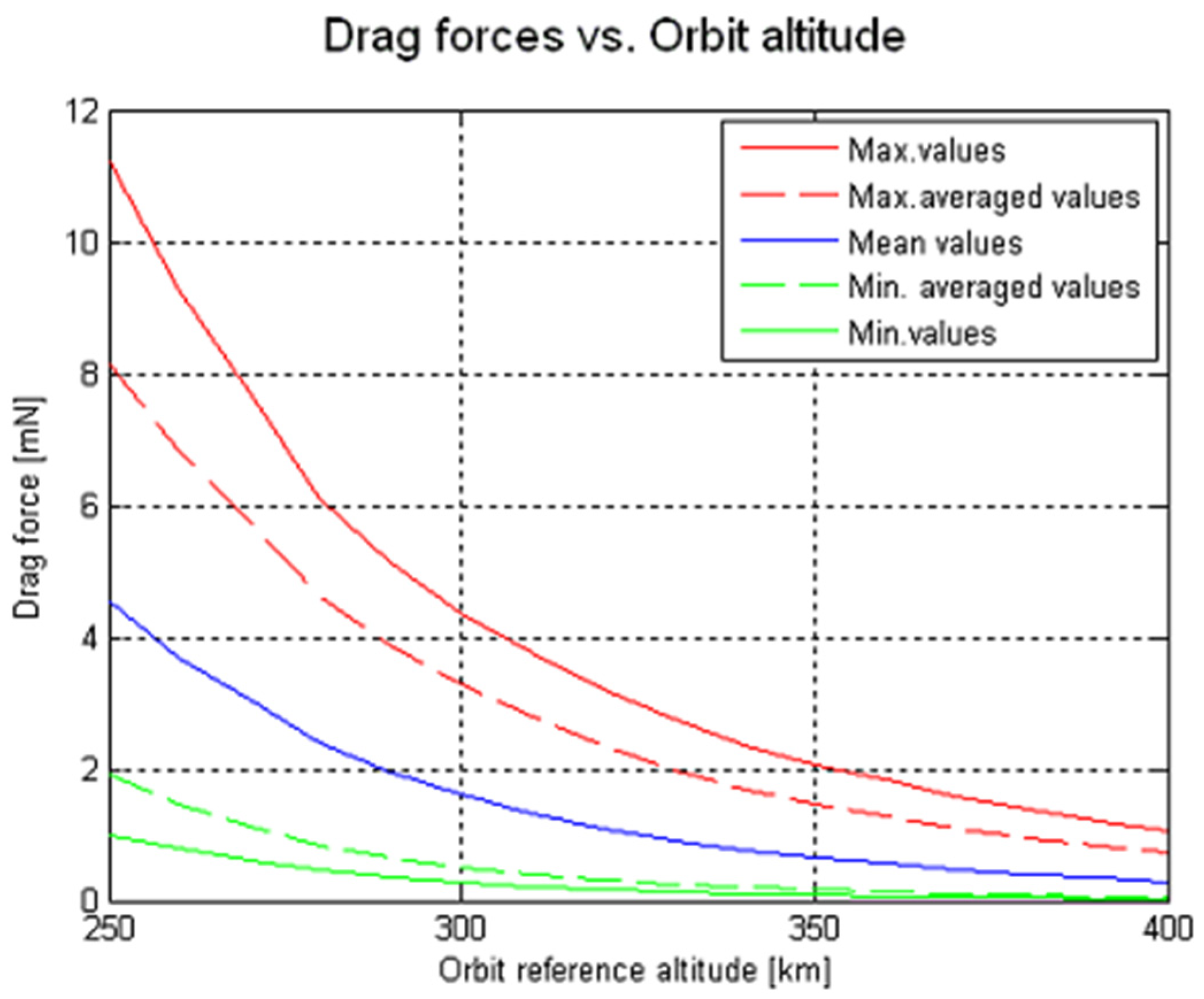
Such new sensors will enable NGGM satellites to orbit at higher altitudes with a fine-tuned intersatellite distance and with a higher sensitivity over a wider range of frequencies, especially at the low end of the science measurement bandwidth. Accelerometer selection and orbit altitude have to be traded off against the need for a drag compensation system. For NGGM, the “drag” experienced by each satellite due to residual atmosphere in the altitude range between 300 and 400 km can be modeled as in
Figure 10, where the in-track drag forces are reverted to accelerations for a GOCE-like satellite of 1 t mass.
Drag accelerations have to be counteracted to ensure a good accelerometer performance and to avoid saturation of the accelerometer measurements. For instance, accelerations of 1–6 × 10
−6 m/s
2 need to be compensated by thrusters on average in case of maximum solar activity. To guarantee the best accelerometer performance, also the cross-track (Y-axis) and radial accelerations (Z-axis), which are one order of magnitude smaller than the in-track drag acceleration, as well as the angular accelerations need to be compensated by the drag-free formation, attitude and orbit control system (DFAOCS). Consequently, all the engineering requirements of
Section 5 have been derived for this worst-case scenario.
One of the current subjects of study is the impact on the system and mission performance when the system design deviates from this scenario, namely when one or more of the engineering requirements are relaxed. As an example, since the errors in the Y- and Z-axis acceleration components only enter the main measurement as projections on the acceleration along the line of sight between the satellites, the corresponding specifications could therefore be relaxed. Some further relaxation of the thrust requirements will result from the concurrent actuation of the magnetic torquers, which are included in the design, as implemented in the GOCE control. Yet another area of investigation is the attitude and pointing control requirements. All these aspects will drive the final design, which will anyway retain, as distinguishing features, at least the along-track drag compensation and the laser beam steering by orienting the satellites. This avoids continuously moving mirrors, which degrade the performance of the measurement of the intersatellite distance (changing the measured optical path and introducing noise in the measurements) and potentially worsen the correction provided by the nongravitational accelerations.
4.2. The Laser Tracking Instrument Preliminary Design
The preliminary SST performances in
Table 5 (top) can an achieved with a laser tracking instrument (LTI), which measures the intersatellite distance variation with a resolution of a few nanometers. The LTI will be a heterodyne Michelson interferometer, which is particularly suitable for measurements over very long distances and operates with continuous wave sources at 1064 nm wavelength (282 THz). As opposed to GRACE-FO, the LTI will be the primary payload of NGGM and specifically designed to match the laser metrology performance, which means that the ultimate performance is due to the instrument and not to other effects, such as a nonoptimal accommodation, environmental effects (e.g., temperature fluctuations) and the dynamic effects of residual air drag.
At present, two interferometer schemes are under evaluation for MAGIC/NGGM. The first is a transponder scheme inherited from the GRACE-FO LRI [
48,
49]. In such an interferometer (see
Figure 11), the laser beam transmitted by the follower satellite (Satellite 2) is received by the leader satellite (Satellite 1) where it is “regenerated” by a second laser source, phase-locked with a frequency offset (heterodyne frequency) to the incoming beam, and retransmitted to Satellite 2. In the optical transponder scheme, a source with limited optical power output of approximately 25 mW, provided directly by the master oscillator, is sufficient to achieve the required signal-to-noise ratio on the photoreceiver. On the other hand, two laser sources must be active simultaneously, one on each of the satellites.
In the second interferometer concept, the optical transponder is replaced by a passive retroreflector on Satellite 1, which intercepts the laser beam transmitted by Satellite 2 and reflects it back. Here, an acousto-optic modulator on Satellite 2 generates the heterodyne frequency, and also the photoreceivers detect the two beat signals produced by the interference of the laser beams: the combination of the photoreceiver outputs produces a sinusoidal signal with a phase proportional to the intersatellite distance variation. The retroreflector scheme (
Figure 12) requires a source with a larger optical power output of approximately 500 mW, which is provided by a fiber amplifier stage after the master oscillator of the same power and quality as in the transponder scheme. In the retroreflector configuration, the acquisition of the optical link between the satellites is significantly simplified: it is sufficient to illuminate Satellite 1 with the laser to obtain the return beam, and no laser frequency scan is necessary to bring the beat signal within the photoreceiver bandwidth. Moreover, by replicating all the interferometer elements on both satellites, these can be made identical, thus realizing a functionally fully redundant system. In case of failure of the active part on Satellite 2, the position of the two satellites along the orbit can be swapped, keeping the same orientation, and the measurement can continue with the interferometer active on Satellite 1. All these features reduce the system complexity and increase its robustness, which are key aspects for an operational gravity mission and motivate a trade-off with the flight-proven optical transponder scheme [
50].
For both concepts, the intersatellite distance variation measurement performance has been assessed via a bottom-up approach in order to verify the compliance to the top-level requirements in
Table 5. For very low orbits of approximately 350 km and intersatellite distances of 100 km, the LTI has to reach an accuracy better than 20 nm/√Hz (threshold) and 10 nm/√Hz (goal) in the measurement bandwidth. The error contributions are split into laser interferometer and spacecraft coupling noise sources as shown in the error tree in
Figure 13.
Each error source has been allocated and estimated as a current best estimate (CBE). The budgets have been computed also for worst-case conditions (WC), when, e.g., the maximum allowed separation between the satellite pair is reached and the measurement is still possible with a minimum amount of received photons. More details on the budgeting for the two concepts can be found in [
50]. Similar to the accelerometer, the errors were combined linearly if correlated and with RSS if uncorrelated, but the LTI overall performance is given by the combination of the error budgets originating from the individual satellites since the LTI instrument is split—in the two different designs—between the satellites of a pair.
The ultimate limiting factor of the performance of both interferometer concepts is the stability of the laser frequency ν, which is the first error source in the budget of
Figure 13: a frequency variation δν induces a distance variation measurement error δd = d·(δν/ν), where d is the distance between the satellites (baseline 100 km). Consequently, to achieve the required accuracy of the intersatellite distance measurement error, the laser frequency stability spectral density of the master oscillator shall be better than 40 Hz/√Hz (threshold) and 20 Hz/√Hz (goal) values [
51]. The required stability can be achieved by locking the frequency of the master oscillator to the resonance of an optical cavity made from low thermal expansion material thermally insulated. Such a frequency stabilization system is now flying on GRACE-FO, and an ad hoc design for NGGM is in progress in the ESA technology program.
5. Single Satellite Pair System Engineering Requirements
The specific NGGM mission and system design will build on the experience of GOCE, in particular for the design of the attitude and orbit control, GRACE, for the concept of SST via precise metrology in low-Earth orbit, and GRACE-FO for the LTI. Whereas
Section 4 focused on the technology selection for the space segment to fulfill user requirements, we derive here the detailed engineering requirements. The NGGM mission requirements were consolidated through a series of system studies and are summarized as follows:
First of all, the scientific instrument of each satellite of the NGGM shall comprise a laser interferometer (or a functional part of it), one accelerometer positioned at the center of mass of the satellite or multiple accelerometers around it, GNSS receivers and a passive retroreflector for laser ranging from the ground.
The operational lifetime for the NGGM satellite pair shall be 7 years as a goal, after a commissioning phase of 6 months for both satellites. Orbiting at a constant mean altitude during the entire mission lifetime is preferred over a variable altitude profile. Phase 0 studies identified that the lowest viable altitude is 340–350 km, which is compatible with the sensitivity requirements (cf.
Table 5) and with the resources needed for orbit maintenance and drag compensation over the complete lifetime. The current baseline of the intersatellite distance is set around 100 km as stated in
Section 4.
The altitude shall be maintained as for the GOCE mission, within a range around a specified value that will be selected to realize a controlled longitude shift of the ground track as described in
Section 3.
The engineering requirements for the satellite design derive from the top-level system requirements formulated in
Section 4.
Figure 14 shows the ASD of the system measurement requirements (threshold and goal) of the fundamental observables of the mission: the intersatellite relative distance variation and the projection of the differential nongravitational acceleration along the satellite-to-satellite direction, based on the ultraprecise accelerometers such as the ones of the GOCE mission (cf.
Table 6).
Successively, the fundamental observables of the mission shall be combined as uncorrelated spectra, as total measurement error ASD in acceleration units (m/s
2/√Hz):
where
(m) is the measurement error ASD of the intersatellite relative distance variation and
(m/s
2) is the measurement error ASD of the differential nongravitational linear acceleration projected along the line joining the satellites’ centers of mass. Alternately, the overall measurement error ASD can be converted in range-rate units (m/s/√Hz):
The system performances for the NGGM pair of satellites are summarized in
Figure 15.
The primary objective of the accelerometer sensor suite on NGGM is to measure the satellite nongravitational acceleration in the satellite-to-satellite tracking direction, with a low-frequency noise (below 1 mHz, where it becomes the dominant error source) possibly better than in GOCE. Several options for accelerometer accommodation are under consideration: one accelerometer is installed in the center of mass, or two (or more) accelerometers can be arranged symmetrically around the center of mass. Moreover, the accelerometers shall provide the measurements on board for the drag-free formation, attitude and orbit control system (DFAOCS) ensuring orbit and formation maintenance, drag compensation, control of the satellite angular accelerations and rates and a high stability pointing of the laser beam.
The internal layout is dictated by the requirement that the optical reference for the intersatellite distance measurement shall be placed in the center of mass and the accelerometers close to and symmetrically accommodated with respect to each satellite center of mass. A stringent temperature stability requirement of
applies in the compartment enveloping the optical bench, where T is the temperature as a function of frequency f, on which all temperature-sensitive items are mounted, including parts of the laser equipment (optical bench assembly and retroreflector) and the accelerometer sensor heads.
The instrument and service equipment boxes (instrument electronics, laser stabilization unit, power control and distribution units, etc.) are accommodated on either side of the central bay, accommodated according to function [
51].
The main driving spacecraft system requirements are associated with the assumptions on DFAOCS and propulsion system. The two systems are fully explained and assessed in the next section.
Enabling Technologies for the NGGM Mission and Derived Control Requirements
The basic requirements of time-variable gravity measurements from space can be realized with a space segment having (a) orbit altitude as low as possible to maximize signal strength, (b) retrieval periods as short as possible to maximize the time resolution of the gravity field solutions and (c) near-homogeneous ground track coverage as dense as possible for each retrieval period (such as a week and a month) for maximum spatial resolution. The lowest possible altitude is dictated by satellite engineering constraints related to the satellite configuration, the cross-section area exposed to air drag, the propulsion type and the amount of propellant. Here, we discuss specific orbit and attitude control solutions that enable formation and ground track maintenance and relative attitude control required by the LTI in the altitude range around 350 km.
The attitude and the environmental disturbing accelerations will be controlled within the frequency range from 1 to 100 mHz according to the derived control requirements in
Table 7. The formation of the two satellites will tend to drift apart under the action of differential air drag and differential accelerometer biases, which can be corrected by commanding a thrust bias as in the case of the GOCE mission [
52]. Dedicated control acting below 1 mHz can ensure that the mean semimajor axis remains within ±100 m of the nominal value and the relative distance is remained within 10% of the nominal intersatellite distance.
The spacecraft propulsion enabling the DFAOCS and orbit control functions is the main challenge of the spacecraft design. For the selected low orbit in the worst-case scenario of average solar maximum conditions, the thrust range and modulation capability imposed by the mission profile, coupled with the lifetime requirement, can likely only be achieved with electric propulsion, which trades propellant mass for electric power. Generating the requested system power of approximately 1 kW is a challenging task for a mission that needs to keep the drag cross-section small (below 1 m²) with high seasonal and orbital variation of the solar aspect angle. Moreover, a high specific impulse is only available over a limited thrust range, and the thrust demand varies by a factor of 3 to 5 during one orbital revolution and even more between the highest and lowest solar activity encountered during the mission lifetime. In the all-electric satellite design, the drag compensation can be enabled by a system of gridded ion engine thrusters of two types, drag control thruster (DCT) and fine control thruster (FCT), which operate in different thrust ranges. The engineering requirements envelope has been derived for each type of thruster in terms of thrust throttling range, specific impulse, total impulse, response time, noise and beam divergence, under ceiling requirements on total propellant mass and total power demand. These are reported in
Table 8 as derived in Phase 0. These will be critically reviewed together with the optimization of the NGGM/MAGIC orbits during the NGGM Phase A. Thrusters meeting these requirements have already been demonstrated in [
53], and FCT backup options encompass flight-proven technologies such as cold-gas thrusters (flown, e.g., on LISA Pathfinder and GAIA) and promising propulsion technologies under development and qualification such as indium-fed FEEP [
54].
For the NGGM application, two 15 mN-class DCT thrusters, in cold redundancy, provide the main force components for the in-line in-band (1 to 100 mHz) drag compensation, formation orbiting control (at frequency below 1 mHz) and orbit maintenance. Two candidate implementations compliant with the requirements exist, and both have flight heritage: The first is the GOCE T5 ion thruster, which can serve—in principle—the same purpose in NGGM. The main difference is that GOCE operated in the thrust range from 70 μN to 20 mN, whereas NGGM requires a thrust range extended at the lower bound since it will orbit considerably higher than GOCE (above 340 km as opposed to 260 km), at the expense of a lower upper thrust limit. Two operating regimes have been specified for the DCT:
Dynamic (throttled) thrust range between 60 μN and 8 mN for the science operations;
Steady-state (unmodulated) thrust of at least 10 mN for the orbit operations such as formation acquisition, collision avoidance and altitude trimming.
A cluster of proportional mN-class FCT microthrusters compensate the drag forces into the cross-track and radial directions and the perturbing aerodynamic torque (for angular drag control purposes), as well as providing attitude and pointing control. The minimal configuration of 8 thrusters offers no redundancy, whereas the fully redundant configuration comprises 16 thrusters. Configurations with 8 thrusters plus 1–2 cold-redundant thrusters have been studied, and other options are possible including 10 operating thrusters with compliant operation in case of one failure and gracefully degraded operation in case of two failures. While the specified minimum operating thrust range is between 50 μN and 1 mN, a reasonably efficient operation below 50 μN and above 1 mN is highly desirable.
The optimal configuration and operation of the FCT system have been intensively studied in the last few years and are still under critical assessment in the MAGIC/NGGM feasibility studies. The following stringent system constraints apply:
The propellant mass for DCT and FCT in combination shall not exceed 100 kg;
The total subsystem peak power for DCT and FCT shall not exceed 350 W;
Both spacecraft shall have an identical thruster layout, keeping in mind that the forces acting on the leading and trailing spacecraft are not identical, while robustly maintaining the laser link;
One or two redundant thrusters shall be able to cope with the failure of any one of the nominal eight thrusters;
The total impulse per thruster shall not exceed the demonstrated lifetime of the candidate technology.
The technology readiness of the entire subsystem, as opposed to the thruster alone, will be a crucial selection criterion during the feasibility studies. Details on the configuration, thruster performances and optimal solution for the redundancy problem are provided in [
51,
53].


