
Metop First Generation AVHRR FRAC SST Reanalysis Version 1


1
NOAA STAR, 5830 University Research Court, College Park, MD 20740, USA
2
Global Science and Technology, Inc., 7501 Greenway Center Drive, Suite 1100, Greenbelt, MD 20770, USA
*
Author to whom correspondence should be addressed.
Remote Sens. 2021, 13(20), 4046; https://0-doi-org.brum.beds.ac.uk/10.3390/rs13204046
Submission received: 25 August 2021
/
Revised: 1 October 2021
/
Accepted: 6 October 2021
/
Published: 10 October 2021
(This article belongs to the Special Issue Remote Sensing Data Sets)
Abstract
:The first full-mission global AVHRR FRAC sea surface temperature (SST) dataset with a nominal 1.1 km resolution at nadir was produced from three Metop First Generation (FG) satellites: Metop-A (2006-on), -B (2012-on) and -C (2018-on), using the NOAA Advanced Clear Sky Processor for Ocean (ACSPO) SST enterprise system. Historical reprocessing (‘Reanalysis-1’, RAN1) starts at the beginning of each mission and continues into near-real time (NRT). ACSPO generates two SST products, one with global regression (GR; highly sensitive to skin SST), and another one with piecewise regression (PWR; proxy for depth SST) algorithms. Small residual effects of orbital and sensor instabilities on SST retrievals are mitigated by retraining the regression coefficients daily, using matchups with drifting and tropical moored buoys within moving time windows. In RAN, the training windows are centered at the processed day. In NRT, the same size windows are employed but delayed in time, ending four to ten days prior to the processed day. Delayed-mode RAN reprocessing follows the NRT with a two-month lag, resulting in a higher quality and a more consistent SST record. In addition to its completeness, the newly created Metop-FG RAN1 SST dataset shows very close agreement with in situ data (including the fully independent Argo floats), well within the NOAA specifications for accuracy (global mean bias; ±0.2 K) and precision (global standard deviation; 0.6 K) in a ~20% clear-sky domain (percent of clear-sky SST pixels to the total of ice-free ocean). All performance statistics are stable in time, and consistent across the three platforms. The Metop-FG RAN1 data set is archived at the NASA JPL PO.DAAC and NOAA NCEI. This paper documents the newly created dataset and evaluates its performance.
1. Introduction
Advanced Clear Sky Processor for Ocean (ACSPO) is the NOAA enterprise sea surface temperature (SST) system. It is currently employed to produce a consistent line of SST products from several AVHRR GAC and FRAC, MODIS, and VIIRS sensors flown onboard low Earth orbiting (LEO; NOAA-7/9/11/12/14/15/16/17/18/19, Metop-A/B/C, Terra/Aqua, and S-NPP/NOAA-20), and ABI and AHI sensors flown onboard geostationary (GEO; GOES-16/17 and Himawari-8) satellites [1,2,3,4,5,6,7,8].
The global AVHRR/3 Full Resolution Area Coverage (FRAC) data, with a nominal resolution ~1.1 km at nadir and ~6 km at swath edge, have been available since the launch of European satellite Metop-A (aka. Metop-2 prior to launch) on 19 October 2006, followed by Metop-B (aka. Metop-1; 17 September 2012) and Metop-C (aka. Metop-3; 7 November 2018). Together, these three satellites comprise the Metop First Generation (FG) series. Under the NOAA-EUMETSAT Initial Joint Polar System (IJPS) partnership, NOAA produces several geophysical products from Metop-FG, including SST. Metop-A will be de-orbited in November 2021 [9]. As of this writing, it remains fully operational, and NOAA will continue producing Metop-A SST until the end of its mission. Although the projected life expectancy of the Metop-FG satellites is only five years, based on the Metop-A experience one may realistically expect that Metop-B/C data will continue well into the 2030s. At the same time, EUMETSAT started transitioning to the Metop Second Generation (SG) series, which will carry a new METImage sensor onboard, with improved SST capability. The first launch is expected in ~2023/24 and Metop-SG is planned to continue into the 2040s. NOAA will produce SST from Metop-SG, under the renewed Joint Polar System (JPS) partnership with EUMETSAT [10]), while continuing its core Joint Polar Satellite System (JPSS; extension of the NOAA heritage Polar Operational Environmental Satellites, POES system) along with Metop-FG SST products [11].
The global FRAC data are well suited for accurate clear-sky masking and high-quality SST retrievals from AVHRR/3 bands 3b, 4, and 5, centered at 3.7, 10.8, and 12 µm, respectively. To prepare for the Metop-SG era, and ensure its continuity with the Metop-FG and POES/JPSS SSTs, the first full consistently reprocessed Metop-FG SST record was created at NOAA with its ACSPO system [1,2,3,4,5]. The first historical reprocessing (RAN1) starts after quality L1b data in the AVHRR infrared bands became available (1 December 2006 for Metop-A, 19 October 2012 for Metop-B, and 4 December 2018 for Metop-C), and continues into near-real time (NRT), with several hours latency. Delayed-mode RAN reprocessing follows the NRT with a two-month lag, resulting in a higher quality and a more consistent SST record. Retrieved SSTs are available in three formats: L2P, L3U, and L3S (e.g., [2,5,12,13] and references therein). All data are archived with the NASA Physical Oceanography Distributed Active Archive Center (PO.DAAC) [14,15,16,17,18,19]. Archival with the NOAA Centers for Environmental Information (NCEI) is also underway. Note that prior to the AVHRR FRAC RAN1, the only Metop-FG SST data which existed were two OSISAF NRT datasets produced by EUMETSAT and also available from PO.DAAC (AVHRR_SST_METOP_A-OSISAF-L2P-v1.0 from 4 June 2013–23 November 2016 [20], and AVHRR_SST_METOP_B-OSISAF-L2P-v1.0 from 19 January 2016–present [21]).
This study documents the AVHRR FRAC RAN1 dataset, with focus on the L2P data. The performance of the L3U data is fully consistent with L2P and not discussed here. The L3S data are documented in [12,13]. Time series of global biases and standard deviations of retrieved SST minus quality controlled in situ SST are analyzed in the NOAA SST Quality Monitor system (SQUAM, [22,23]). The in situ SSTs from drifting and tropical moored buoys (D + TM) and Argo floats (AF), employed in the calibration and validation (Cal/Val) of satellite data, come from another NOAA system, in situ SST Quality Monitor (iQuam, [24,25]). Consistency checks against the Canadian Met Centre Level 4 analysis (CMC L4 SST) are also performed in SQUAM, including analyses of clear-sky fraction (percent of SST pixels to the total ice-free ocean pixels; cf. prior analyses for AVHRR GAC RANs [2,8,26]). Quality of the ACSPO Clear-Sky Mask (ACSM) and SST imagery, as well as the newly derived thermal fronts product, are monitored in the NOAA ACSPO Regional Monitor for SST system (ARMS [27]).
2. ACSPO Algorithms
ACSPO generates two SST products, one with the global regression (GR) and the other with the piecewise regression (PWR) algorithms. Both algorithms are regressions trained against in situ SSTs obtained from (D + TM), with the GR trained in the full retrieval domain and the PWR separately in its multiple segments. Note that the GR SST is also referred to as the subskin SST since it is highly sensitive to spatial and temporal variations in skin SST, TSKIN, being at the same time globally unbiased with respect to in situ (depth) SST, TIS [4]. The ACSPO GR subskin SST is produced similarly to the OSISAF Metop FRAC subskin SST product [28], i.e., by direct training against in situ data. (This is in contrast with the ‘skin’ SSTs, produced by other retrieval systems, which either train the regression against in situ SST and then subtract 0.17 K [29], or employ physical retrievals which should result in ‘skin’ SST.) The PWR SST, on the other hand, is less sensitive to TSKIN, but more precise with respect to depth TIS [3]. Due to its superior accuracy and precision of fitting TIS, the PWR serves as a proxy for ‘depth’ SST, TDEPTH. The GR SST is reported in the ACSPO L2P GDS2 files in the ‘sea_surface_temperature’ layer, whereas the ‘SSES_bias’ layer reports the difference between the GR and PWR SSTs. One can obtain the PWR SST by subtracting the ‘SSES_bias’ from the GR SST. (Correspondingly, the PWR SST is also referred below as the ‘Debiased’ SST).
Both ACSPO SSTs are calculated during day- and nighttime with different, two- and three-band regression equations, respectively, with the switch-over occurring at the solar zenith angle = 90°. The daytime two-band SST equation takes the following form:
The nighttime three-band equation is written as follows:
Here, T3.7, T11 and T12 are AVHRR brightness temperatures (BTs) at 3.7, 10.8, and 12 µm;
, is satellite view zenith angle (VZA); and are regression coefficients; and are offsets. is the first-guess SST obtained by interpolating the gridded L4 analysis to AVHRR pixels (note that RAN1 employs the Canadian Meteorological Center Level 4 analysis, CMC L4 SST [30]).
The GR SSTs use daily-recalculated, globally non-variable sets of coefficients, one for day and another one for night. Both are trained against (D + TM) in the corresponding global data sets of matchups (MDS). The PWR SST uses multiple sets of coefficients, also recalculated daily but trained against subsets of matchups, whose vectors of regressors, R, belong to specific segments in the space of regressors (R-space). The total number of segments, into which the R-space is subdivided, is 320. The PWR coefficients are calculated for a given segment, if the corresponding subset includes at least 100 matchups. Otherwise the GR coefficients are used. To avoid discontinuities in the PWR SST, its coefficients are interpolated between the neighboring segments in the R-space. Detailed description of the PWR algorithm can be found in [3]. During the retrieval, the PWR coefficients at a given pixel are selected by the value of R.
Note that Equations (1) and (2) include more terms than the OSISAF equations [28]. Increased number of regressors is intended to extract maximum information from the satellite observations. The risk of adding more regressors in the equation, however, is that due to increased correlations between them within the training MDS, the estimated coefficients, produced with the conventional least-squares method, may become unstable. This risk is minimized with the method documented in [31], which reduces the dimensionality of the subspace, in which the vector of coefficients is estimated, by cutting off the least informative dimensions in the R-space. This is aimed at extracting maximal information from the regressors, while stabilizing the estimates of the coefficients.
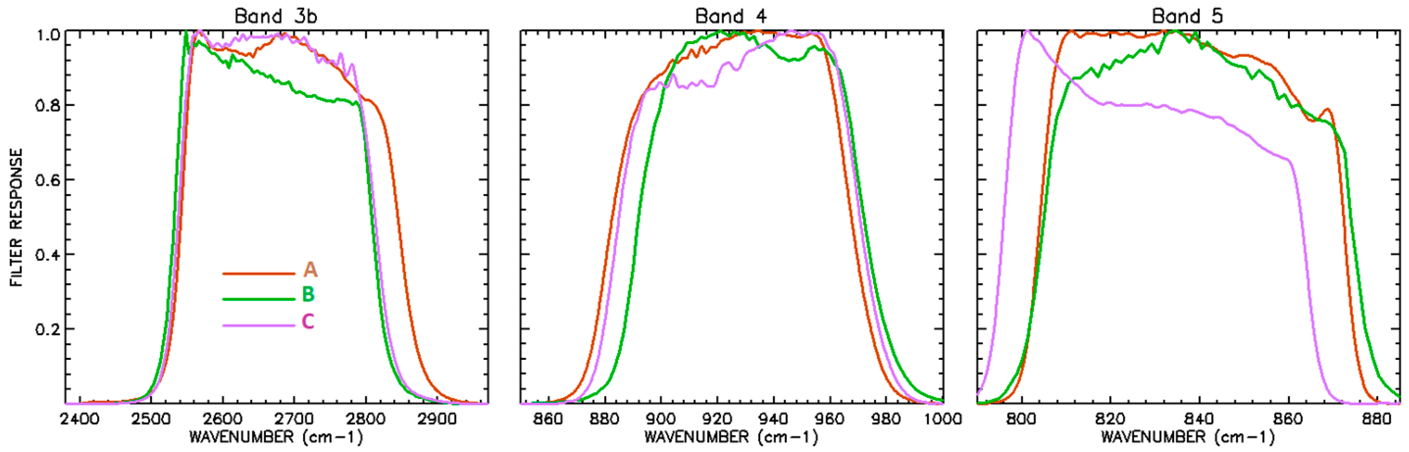
Equations (1) and (2) both follow the conventional NLSST approach [32] by including regressors depending on T0. The global correlation between the T0 and TIS is usually very high (>0.9), and the inclusion of T0-dependent regressors in the GR equation improves precision of fitting TIS with TS. However, the improved precision is even more noticeable in the PWR SST (where the correlations of T0 with TIS are generally lower over segmental subsets of matchups than within a global MDS). This is due to the fact that the same number of predictors is applied over a limited set of atmospheric and SST conditions, where a priori SST variability is reduced compared to the global MDS. The drawback of using T0-dependent regressors is that the retrieved TS becomes sensitive to T0, while its sensitivity to the ‘true’ TSKIN may degrade, if not controlled during the training process. Note that the concept of sensitivity to ‘true’ SST was introduced in [33]. Sensitivity varies across the full retrieval domain, and defines how well the spatial and temporal contrasts in the ‘true’ TSKIN are captured in the retrieved satellite SST, TS, in each pixel (ideally, it should be = 1). According to [34], the global mean nighttime sensitivities of the ACSPO GR SSTs are ~0.97 for Metop-A and ~0.94 for Metop-B/C. The corresponding daytime statistics are ~0.89 for Metop-A, ~0.88 for Metop-B and ~0.87 for Metop-C. The small differences between the three Metops likely result from different AVHRR spectral response functions (SRFs; shown in Figure 1) [35].
Although the regression coefficients are individually trained for each satellite sensor against the same iQuam (D + TM) SSTs, different SRFs may result in slightly different performance of the corresponding SSTs. Nevertheless, as it will be shown later, the cross-platform SST differences are small and do not affect their global performance statistics in any statistically significant way.
In contrast with the GR SSTs, the mean sensitivity of the PWR SSTs is controlled during the training. The segmental coefficients are initially calculated using a standard least-squares method. If the mean sensitivity in a given segment is less than 0.4, then the coefficients are recalculated with the segmental mean sensitivity constrained at 0.4, using the method [31]. The global mean sensitivity of the resulting PWR SSTs is close to ~0.6.
The clear-sky identification is performed with the ACSPO Clear-Sky Mask (ACSM), which employs a set of threshold-based filters [1]. The following four filters use retrieved SSTs and measured BTs in the individual AVHRR IR bands as predictors:
- SST filter (includes static and adaptive parts);
- Warm SST filter (for low stratus clouds);
- Low stratus filter (proved a useful addition to the ‘Warm SST filter’ above);
- Spatial uniformity filter.
The above four filters are used during both day and night. During the daytime, the ACSM also includes three additional filters:
- 5.
- Reflectance Relative Contrast filter;
- 6.
- Reflectance Gross Contrast filter;
- 7.
- SST/Reflectance Cross-Correlation filter.
Filters 5 and 6 use AVHRR reflectance bands 1 (0.63 µm) and 2 (0.87 µm). Filter 7 exploits cross correlation between the band 1 reflectance and GR SST. All filters are binary, with output being either “clear” (usable for SST) or “cloudy” (unusable for SST). The definition of quality levels in ACSPO is based on the ACSM individual bit flags. Only pixels with QL = 5 (assigned when all filters are set to “clear”) are recommended for use, in all applications.
3. Variable Regression Coefficients
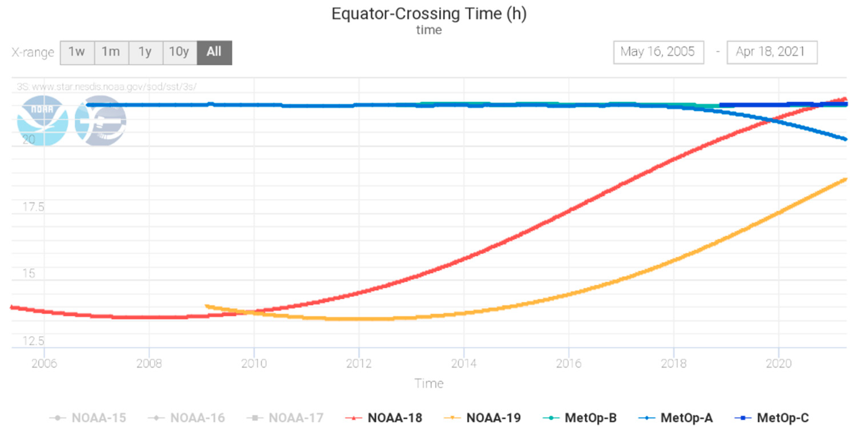
Metops are maintained in stable ‘mid-morning’ orbits, with local equator crossing times, LEXTs~9:30 am/pm. This is achieved by performing periodical orbital corrections, using available fuel onboard. (Note that the NOAA satellites comprising the US heritage POES constellation, have no fuel onboard and basically operate in a ‘free-falling’ mode, immediately after launch [36].) Figure 2 shows LEXTs for the three Metop-FG satellites, and for the two most recent POES satellites, NOAA-18 and -19. The NOAA-18 and -19 were launched in May 2005 and February 2009, respectively, into the standard POES ‘afternoon’ orbits with LEXT~1:30 am/pm, however, their LEXTs have significantly drifted since then. In particular, by August 2021, NOAA-18 crossed the equator around LEXT~10 am/pm, later than Metops, whereas the NOAA-19 still flied at ~7 am/pm, progressing towards the nominal 9:30 am/pm Metop orbit [35,36,37]. The major Metops’ advantage is that they observe ocean at about same local time during many years in space, thus minimizing the effect of the diurnal cycle on retrieved SST, whereas the POES satellites move through almost full diurnal cycle during their shorter lifetimes. The Metop-A satellite ran out of fuel in September 2016, and its orbit has not been controlled since then, making it a ‘free-falling’ object like all POES satellites [37]. The drifting POES orbits were a major motivation for using variable regression coefficient in AVHRR GAC RAN1 [2]. From the LEXT perspective (except for the past several years of Metop-A life), the need for those in Metop RAN is not as compelling as it was in POES RAN.
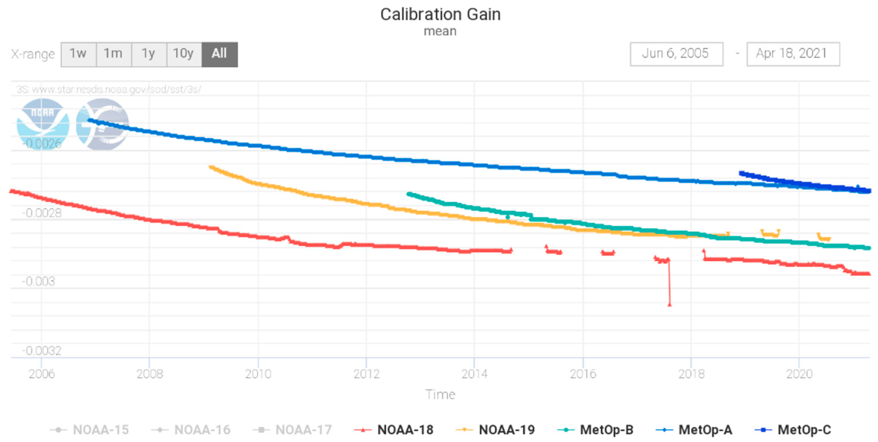
Another motivation for using variable regression coefficients in the GAC RAN1 was the well-known instability of the AVHRR sensors onboard POES satellites (e.g., [37] and references therein). In addition to flying in stable orbits, the bigger Metops provide better housing for the AVHRRs. Together, these two factors are expected to lead to an overall more stable AVHRR performance. Figure 3 shows the nighttime gains in one of the AVHRR/3 bands used for SST, 3b, for the three Metop and two POES satellites. Systematic degradation takes place in all five AVHRRs, due to apparently similar processes of ageing their fore optics, mirrors, and the overall sensor optical tracts. The changes on Metops are smoother and more predictable, whereas the two POES AVHRRs show frequent irregularities superimposed on the top of smooth degradation, in particular around the missing nighttime data (which occur when the NOAA satellites fly in all-Sun orbits, and do not go into Earth’s shadow during extended periods of time, up to several months).
Time series of LEXTs and calibration gains provide a suggestive, yet indirect and incomplete, evidence of sensor stability. Some other factors are not controlled or accounted for in the calibration algorithm. For instance, the sensor SRFs may change during many years in space. Immediate inputs into SST algorithms are BTs, and their time series provide more direct verification of sensor stability for SST. The differences between the observed BTs and those simulated with the Community Radiative Transfer Model (CRTM) [39] (‘O-M biases’) are monitored in the NOAA Monitor of Infrared Clear-sky Radiances over Ocean for SST (MICROS; [34,40]).
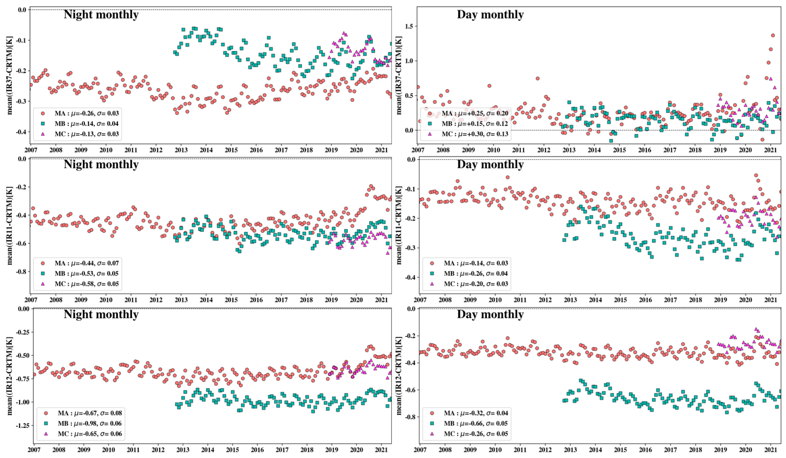
Full-mission time series of Metop-FG O-M biases are shown in Figure 4 (including the 3.7 µm band during the daytime, which however is only used for SST at night).
Note that systematic negative offsets in the O-M biases are expected, due to two factors in the ‘M’ (using warmer depth CMC L4 SST, instead of cooler skin SST, and unaccounted aerosols) and one factor in the ‘O’ (possible residual cloud in the observed clear-sky BTs) [40]. On average, the AVHRR L1b calibration algorithm efficiently mitigates the effect of smoothly degrading sensor gain, as expected. The O-M biases in different bands and on different satellites often vary in sync (cf. the well-expressed seasonality in all bands of all satellites). This is due to the inputs in the ‘M’ (CMC L4 SST and Global Forecast System, GFS atmospheric profiles. For instance, the difference between satellite skin and CMC depth SSTs varies regionally and seasonally). Some bands of some sensors (e.g., Metop-B band 12 µm) are out of family, possibly due to their incorrectly calculated CRTM coefficients (e.g., if their SRFs were measured incorrectly pre-launch, or CRTM coefficients were in error, due to some other reason) [40]. Errors in the ‘M’ (including such correlated and/or systematic) do not affect SST. However, when the O-M biases show significant multidirectional and inconsistent (uncorrelated) variations (between different bands, sensors, and day/night), those are due to the ‘O’ term (i.e., remaining sensor calibration or characterization issues) which directly affect SST retrievals. Favorably for Metops, such uncorrelated variations in their O’s are much smaller than they were in the NOAA GAC data (whose effect on SST was corrected in AVHRR GAC RAN1 using variable regression coefficients [2]).
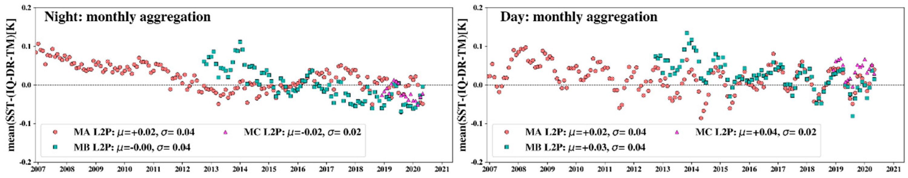
As in the AVHRR GAC RAN1 [2], we first tried to use a fixed set of coefficients for an initial version of Metop-FG RAN, and processed complete time series. Figure 5 shows the resulting monthly global mean biases in GR—(D + TM) SSTs. Typically, the ΔTs are within a ~±0.1 K corridor, and well within the NOAA SST accuracy specifications of ±0.2 K (cf. ~±0.2 K corridor in the AVHRR GAC SSTs derived with fixed coefficients [2]). However, the systematic trends in the ΔTs time series, and the remaining inconsistencies across individual platforms, suggest that they are attributed to variable biases in satellite BTs, and variable SST coefficients should mitigate them. The ‘initial’ L2P SST retrievals shown in Figure 5, were used to collect matchups of clear-sky AVHRR BTs with in situ SSTs, from which a set of variable regression coefficients was derived. This process was repeated several times, until the biases in Ts with respect to TIS were minimized, stabilized and reconciled. The remainder of this paper shows that using variable coefficients indeed significantly improves the stability of the SST time series, and their cross-platform consistency.
The variable regression coefficients for the GR and PWR SSTs are trained against matchups with (D + TM) collected within a limited time windows around the processed day. The size of time window is 91-day for the GR and 361-day for the PWR SSTs. The larger window size for the PWR SST is intended to provide sufficient numbers of matchups for specific segments in the R-space. The offsets of the GR and PWR equations are additionally corrected using a shorter time window of 31-day size. In RAN, all training windows are centered at the processed day. In the NRT processing, the training windows are of the same size, but cover a period ending four to ten days before the processed day. The data, processed in the NRT mode, are reprocessed later in the RAN mode, with a ~two-month lag. Note that using variable regression coefficients does not affect the standard deviations with respect to in situ data, and only serves to stabilize the corresponding mean global biases, ΔTs = Ts − TIS.
4. Validation
In this section, Metop FRAC SSTs are consistently validated against (D + TM) and AF data from the NOAA iQuam system, using matchups collected within 10 km × 30 min window. All satellite SST pixels in this window are matched up with the central in situ anchor, forming a “one-to-many” MDS. Each pair in the MDS is considered an independent match-up.
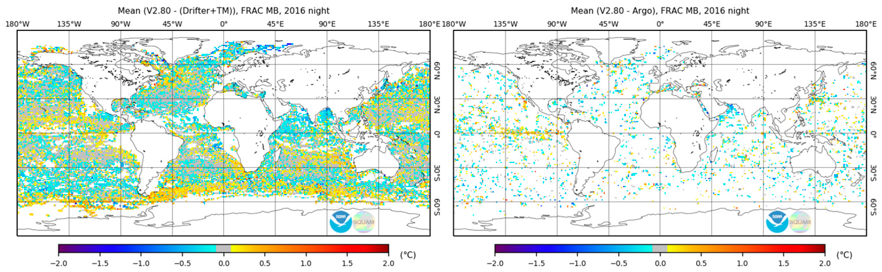
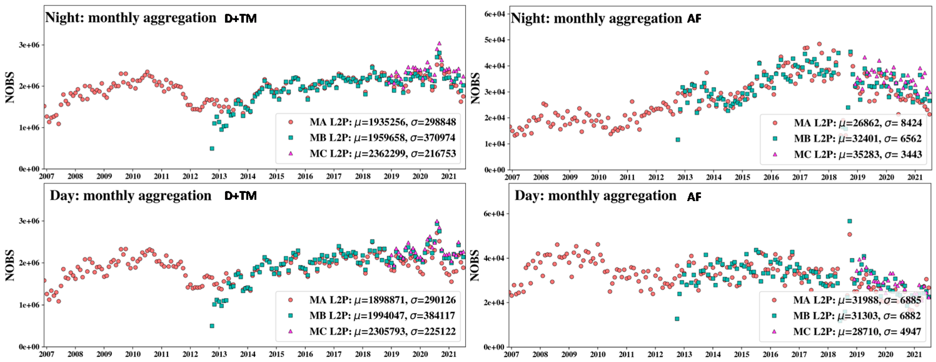
Figure 6 shows representative examples of nighttime yearly aggregated maps of GR—(D + TM) and GR—AF SSTs for Metop-B in 2016. The coverage by the (D + TM) matchups is close to uniform and globally representative (except in some areas with persistent cloud and heavy aerosols—e.g., off the west coasts of the South/North Americas and Africa, and tropical warm pool). Coverage with the AFs matchups is more uniform, although two orders of magnitude sparser (cf. the number of observations, NOBS, in Figure 7).
4.1. Validation against Drifters and Tropical Moorings (D + TM)
Note that the (D + TM) are used to train both GR and PWR regressions, and recalculate their coefficients in time, which maximally reconciles global satellite and in situ SSTs. Validation against the same in situ data is not fully independent, and may appear non-informative and even self-deceiving. We emphasize that it is still critically important, from several perspectives. It helps to verify that the selected sets of regressors and the training methodology are both adequate (i.e., the satellite data and adopted equations allow accurate fitting of the in situ data, with minimal regional and temporal biases). Note that daily recalculation of the regression coefficients (“calibration”) only minimally and statistically insignificantly affects the global standard deviations (a measure of SST regional biases). Also, using wide time windows for “calibration” results in non-zero (but small) global validation biases for each individual day. The global statistics vs. (D + TM) are also informative to compare the relative performance of the PWR and GR SSTs. Note also that compared to the AFs, the (D + TM) measure SST closer to the skin SST, sensed from the satellite, and cover a wider global domain (including improved coverage in the high latitudes), more densely and with more details. Moreover, availability of both (D + TM) and AF validation results allows one to check for qualitative and quantitative consistency between the dependent and independent in situ standards.
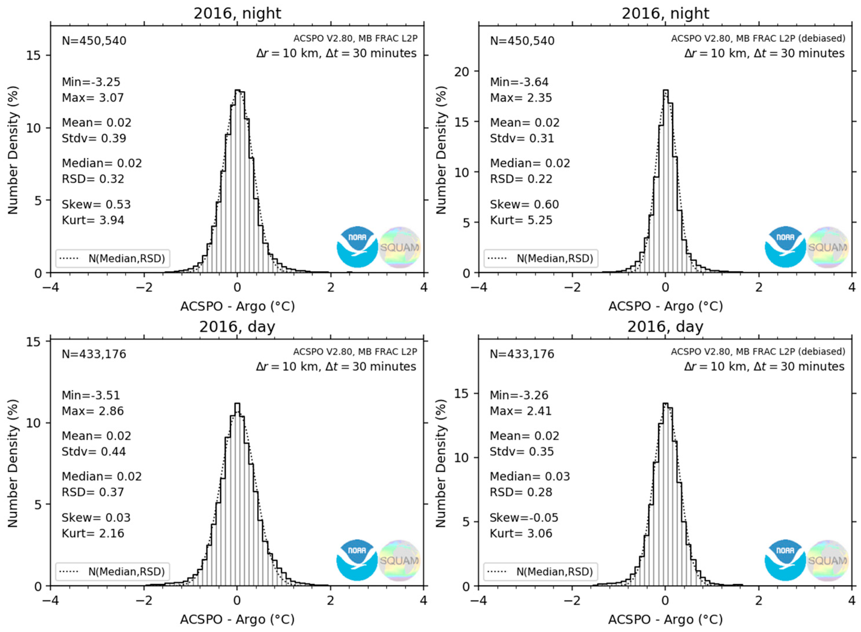
Figure 8 shows yearly histograms of nighttime and daytime GR—(D + TM) and PWR—(D + TM) SSTs for Metop-B in 2016. All histograms are close to Gaussian. The daytime distributions are wider than the nighttime ones, likely due to degraded performance of the daytime split-window two-band SST equation, compared to the nighttime three-band, and increased diurnal signal during the day. The histograms for the PWR (depth) SSTs are significantly narrower than for the GR (subskin) SST, as expected. The yearly statistics are based on ~24 million matchups and are statistically significant and globally representative. The results for Metop-A and -C (not shown) are largely consistent with Metop-B shown in Figure 8.
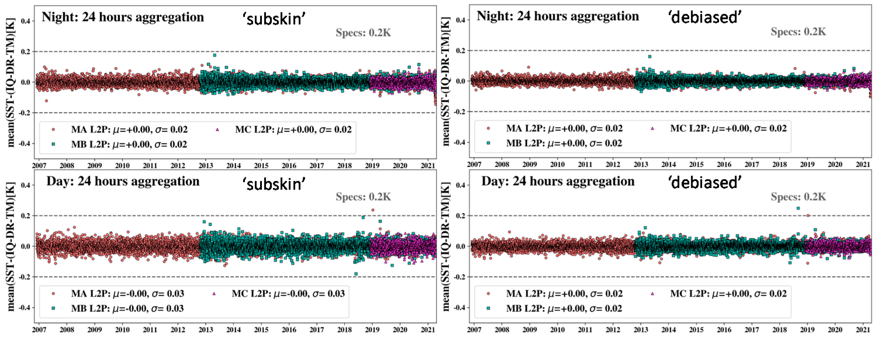
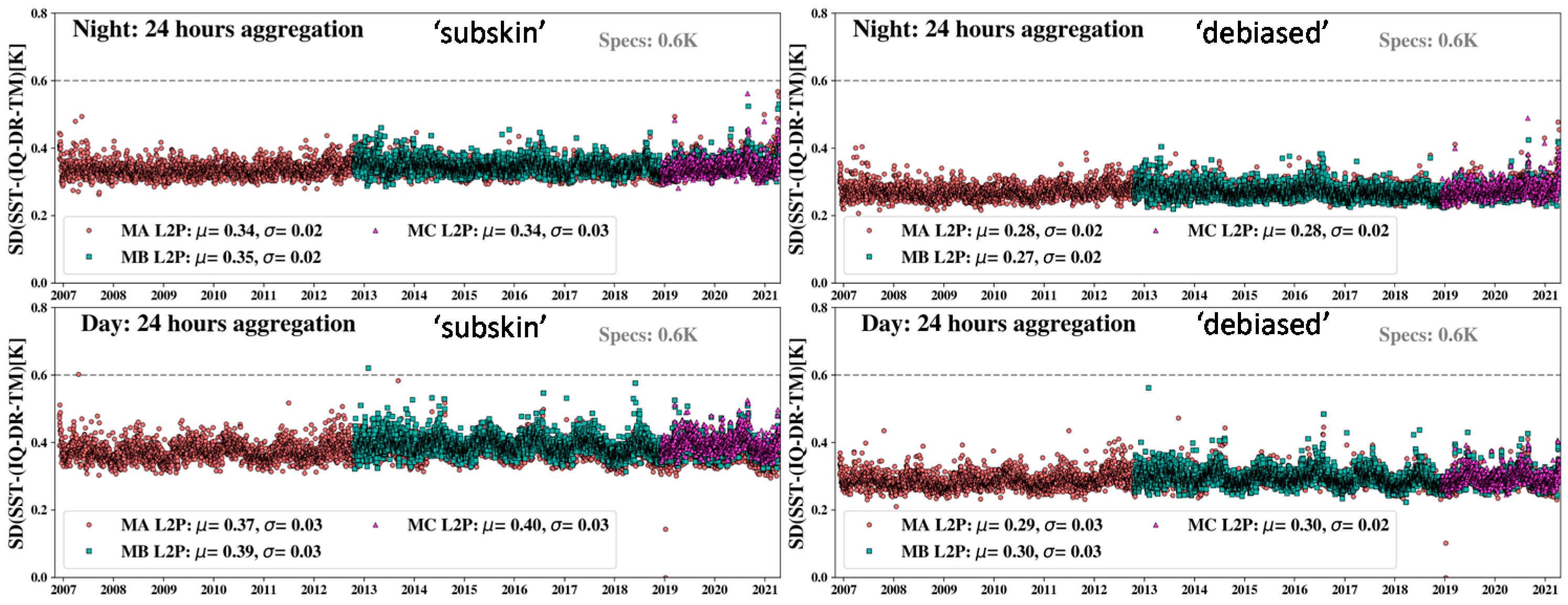
Figure 9 and Figure 10 show full Metop-FG time series of the 24-h aggregated global mean biases and SDs with respect to (D + TM). NOAA SST requirements are ±0.2 K for the accuracy (global mean biases wrt. in situ data) and 0.6 K for the precision (corresponding SDs). Both nighttime and daytime biases are stable and meet the NOAA specs, with a wide margin. The PWR SSTs are more consistent with (D + TM), with biases being closer to zero and forming a tighter cluster than for the GR SST. The SDs are also consistent across all three satellites, for both GR and PWR. The daytime and nighttime SDs compare favorably with the NOAA specifications, with the PWR SDs exceeding the NOAA requirements with a wider margin. Seasonal variations in the daytime SDs in Figure 10 are caused by the regional and seasonal differences in the diurnal warming cycles between the subskin and in situ depth SSTs.
4.2. Validation against Argo Floats (AF)
The AFs were not used for the training of the regression SST equations and thus represent an independent validation data set. Figure 11 shows histograms against AFs, similar to those against (D + TM) in Figure 8. Their shape remains near-Gaussian, but with slightly positive biases, due to the (D + TM) being closer to the surface (~0.2–1.0 m) and warmer than the ~6 m-deep measurements from the AFs.
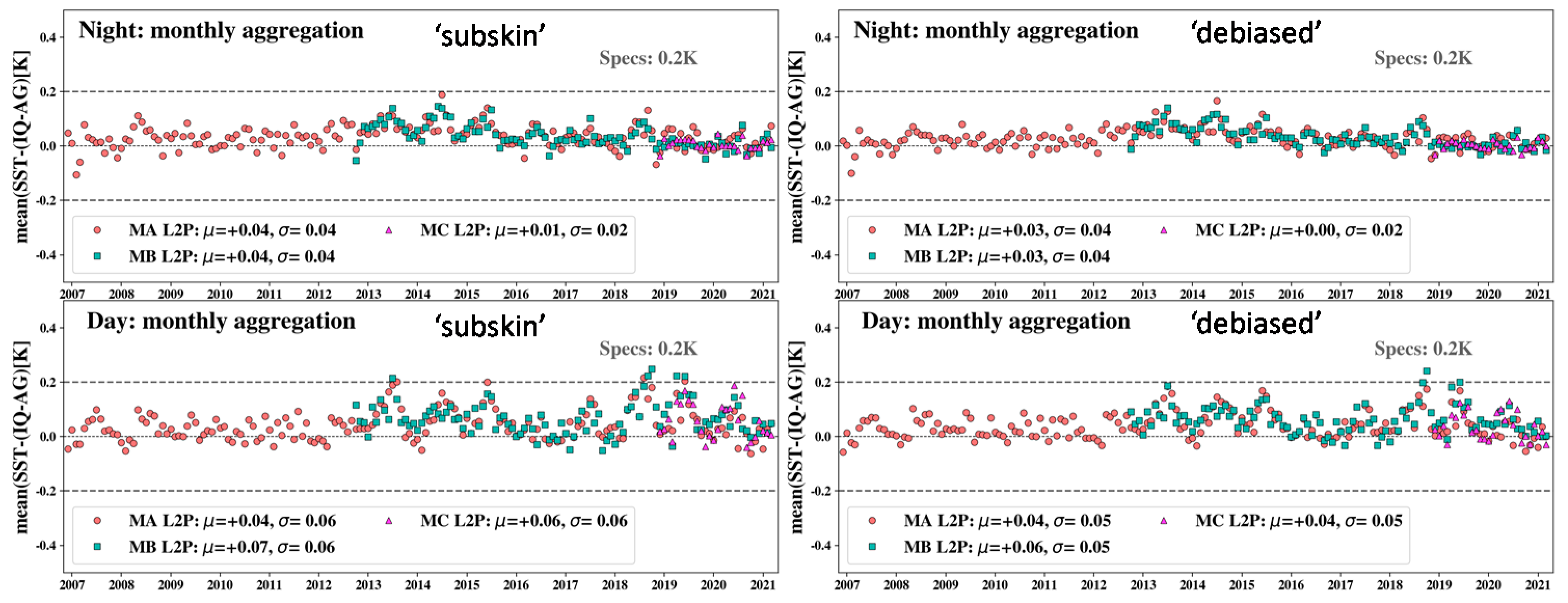
Figure 12 and Figure 13 show the time series of the monthly global mean biases and corresponding SDs, with respect to AFs.
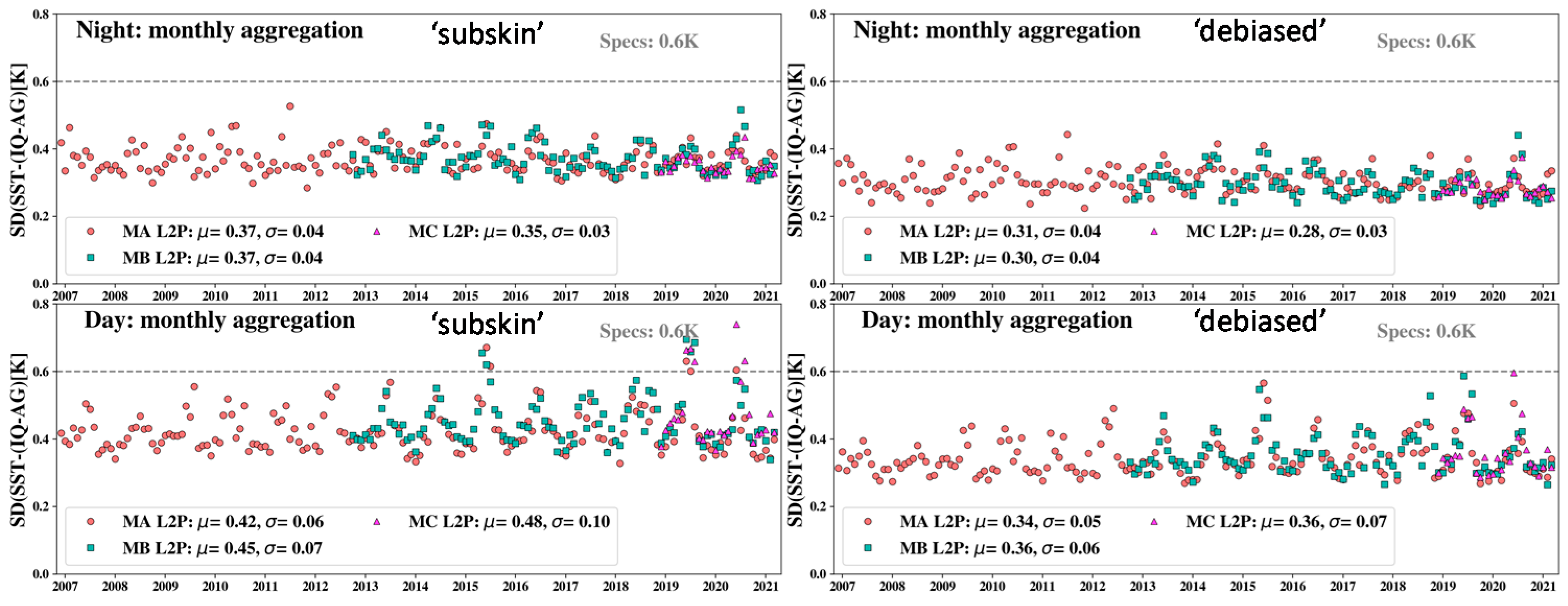
Both the GR and PWR SSTs are on average 0.03–0.04 K warmer than the AFs (cf. ~+0.02 K biases in Figure 8), due to training against slightly shallower and warmer (D + TM). The AF validation statistics continue showing seasonal cycle, due to different phasing of the SST diurnal thermocline in the Northern and Southern Hemispheres. Despite AF monthly aggregation (vs. daily for the D + TM, to mitigate their approximately two orders of magnitude different daily NOBS), all AF statistics are noisier than their (D + TM) counterparts. Two major factors are deemed to be contributing to the increased noise: AF’s being independent from, and most importantly, measuring much deeper than the (D + TM). Typical SDs of the GR SST wrt. AFs (0.35–0.37 K at night and 0.42–0.48 K during the daytime) are increased from the corresponding (D + TM) statistics (0.34–0.35 K at night and 0.37–0.40 K for the day). The same trends are seen in the PWR SST: 0.28–0.31 K (AF) vs. 0.27–0.28 K (D + TM) at night, and 0.34–0.36 K vs. 0.29–0.30 K during the day. Importantly, the validation against fully independent AFs remains largely within the NOAA requirements, and consistent across all three platforms.
5. Consistency with CMC L4
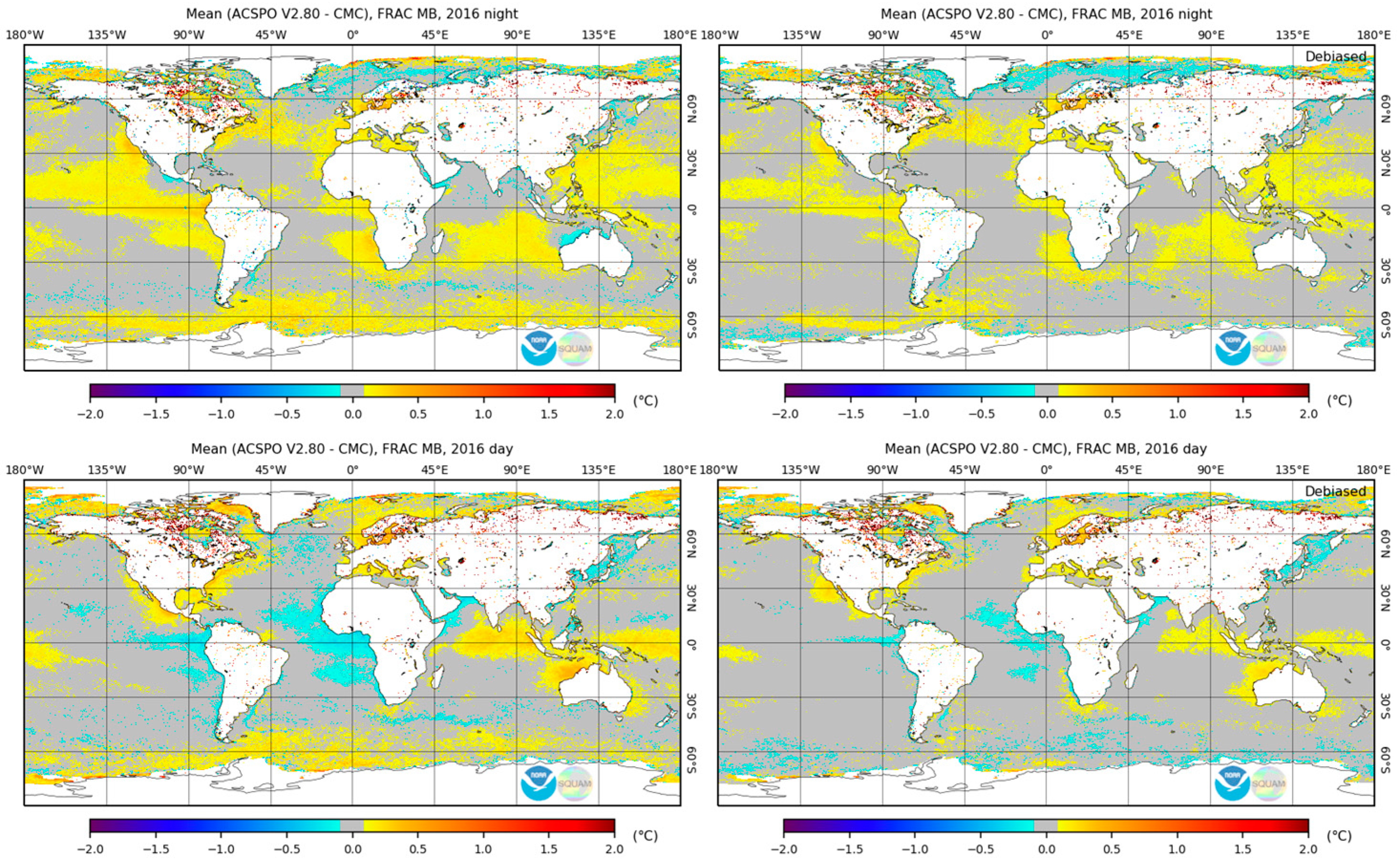
Figure 14 shows example yearly composite maps of Metop-B ACSPO—CMC L4 SST in 2016, for night and day. Note that the CMC L4 analysis currently does not assimilate the ACSPO Metop data. Being a fully independent dataset, the CMC L4 product is thus appropriate for additional verification of the newly derived Metop-FG SST dataset.
Overall, the ACSPO Clear-Sky Mask (ACSM) is efficient in preventing significant cloud leakages in retrieved SSTs. However, suppressed GR SSTs (with ΔTS < −0.1 K) are seen in the Arabian Sea, off the West Africa, South America, East Asia, and South Australia. All these areas are characterized by persistent cloud and elevated aerosols, and the ACSM may miss some of those. The ACSPO PWR (depth) SST successfully mitigates many of these coldish spots and is closer to the ‘foundation’ CMC L4 SSTs than the GR (subskin) SST, as expected. In some cases, however, the PWR SST is biased colder than the GR (high latitudes in both Northern and Southern Hemispheres). It is not immediately clear what product represents the true SST more closely, and more analyses are needed to validate SST at the high latitudes.
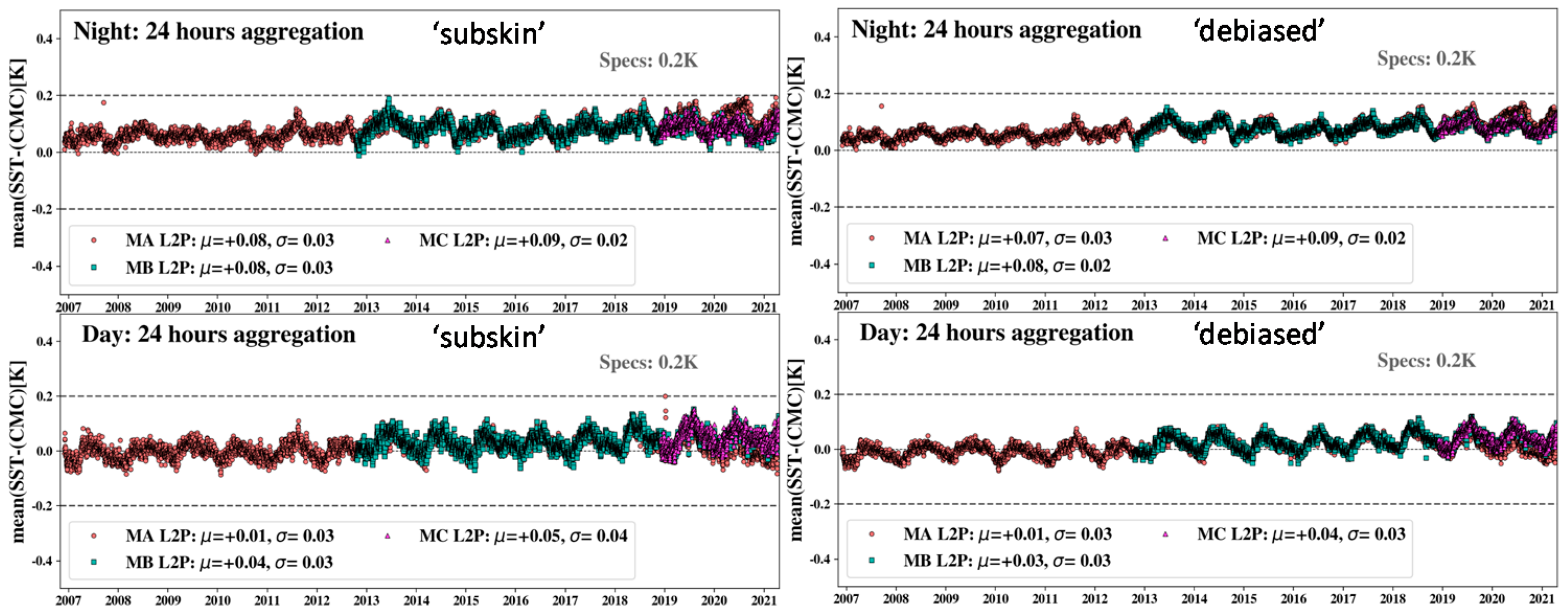
Figure 15 shows time series of the global mean biases wrt. CMC L4 SST. At night (~9:30 pm local time, LT), ACSPO SST closely agrees with the ‘foundation’ CMC L4 SST during the boreal winters. However, during the boreal summers, it develops seasonal warm biases up to ~0.2 K (likely due to residual diurnal warming at ~9:30 pm, during the periods when the insulation during the daytime is high and wind mixing suppressed). The daytime (~9:30 am LT) biases are centered at ~0 K. The PWR SSTs exhibit the same seasonality as the GR SST, except the three Metops are now clustered much tighter. Being ‘depth’ SST, it is expected to agree better with the ‘foundation’ CMC L4. Metop-A starts deviating from the daily CMC L4 SST in recent years, due to its orbital shift from 9:30 am/pm in 2016 to ~8 am/pm in August 2021.
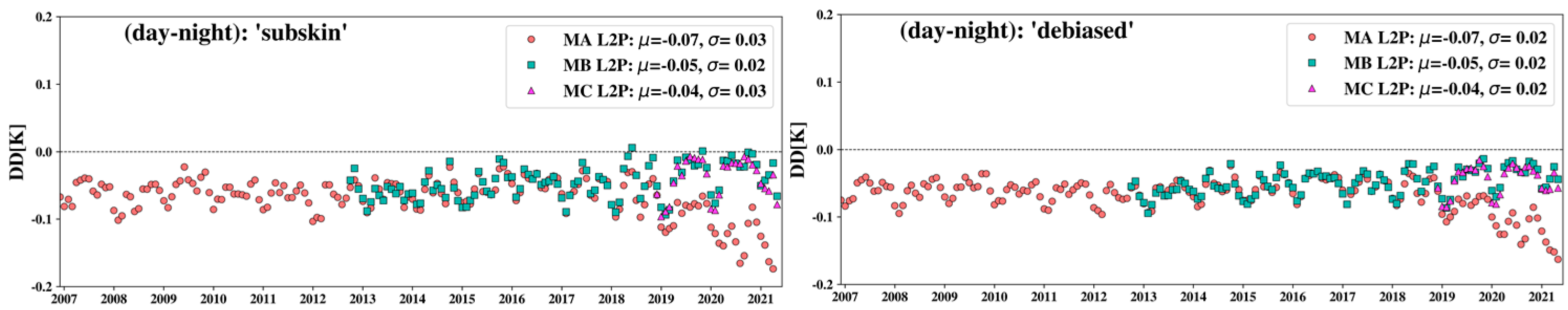
Figure 16 shows the global Double Differences, defined as DD = [(ACSPO day—CMC L4 SST)—(ACSPO night—CMC L4 SST)]. Note that DDs are widely used in climatology and sensor calibration communities (e.g., [40] and references therein), to compare statistics of the two fields measured in different domains. The CMC L4 SST being subtracted from the day and night SSTs, largely cancels out and leaves DD representing the diurnal signal in satellite SSTs. The DD ~−0.05 K suggests that globally, daytime SST at ~9:30 am LT is on average 0.05 K cooler than nighttime SST at ~9:30 pm LT. Apparently, some residual diurnal warming still remains at 9:30 pm, which subsequently cools off over night, and does not warm up as much before the 9:30 am. This demonstrates the potential of the Metop-FG SST to measure a subtle diurnal change and its stability over time. The other impressive characteristic is capturing the increasing Metop-A DD after year 2018, due to its de-orbiting and shifting LEXT to the earlier hours (~8 am/pm as of August 2021 [38]). Cooling between 8 pm and 8 am is even larger, up to >0.10 K, due to larger diurnal residual remaining at 8 pm. Diurnal signal in the PWR SST is comparable to that in the GR SST, but less noisy, and more cross-platform consistent.
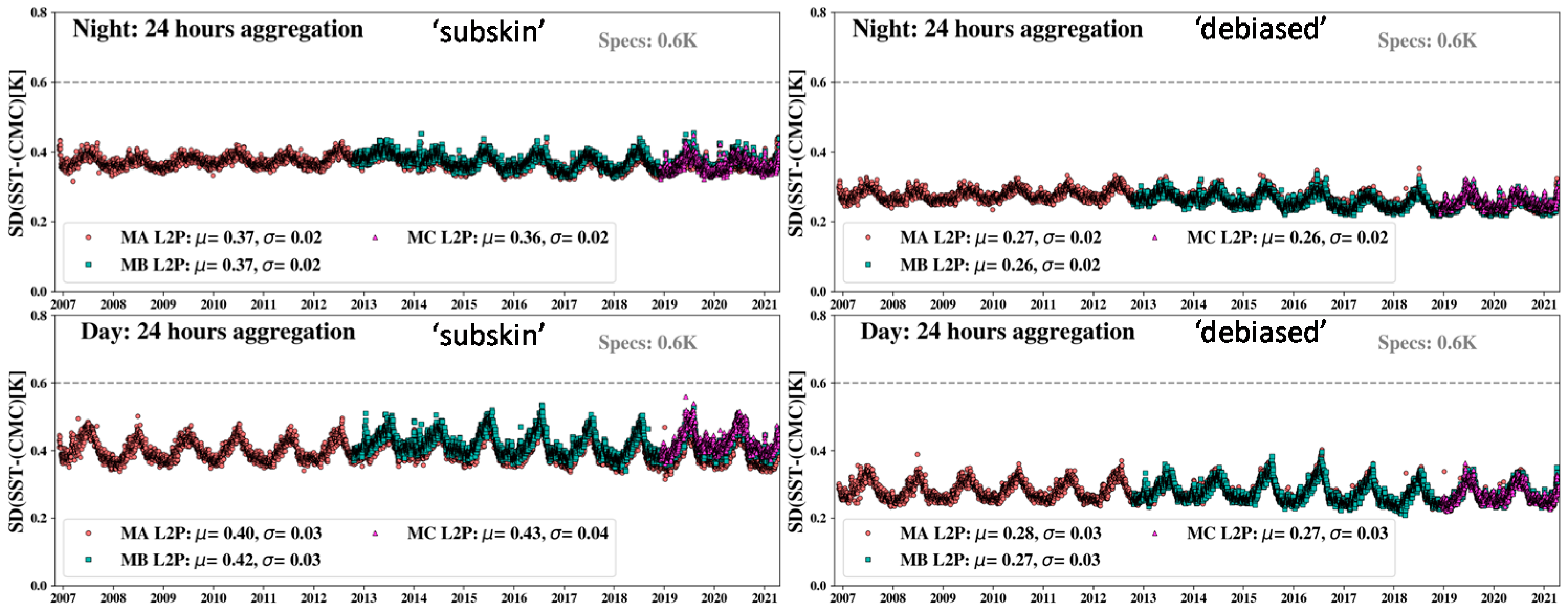
Figure 17 shows SDs of ACSPO—CMC L4 SST (corresponding to mean biases in Figure 15). All time series are stable in time, suggesting that the ACSPO L2P and CMC L4 datasets are very consistent, while being fully independent. The SDs of the PWR SSTs are noticeably smaller than for the GR SST, and form tighter clusters across the three satellites.
Figure 18 shows the time series of nighttime and daytime clear-sky fractions (i.e., the percent of clear-sky pixels, identified by the ACSM, to the total of ice-free ocean pixels). The daily clear-sky fractions are consistent across three platforms (at ~20–22%, on average) and show an approximately ±2% seasonality. Note that NOAA requirements for SST coverage are 18%, and the Metop-FG RAN1 product fully meets it.
6. Latitudinal Hovmöller Diagrams of Biases with Respect to (D + TM)
Time series presented in Section 4 and Section 5 suggest that the global statistics of the ACSPO Metop FRAC SSTs are stable in time and consistent across three platforms. This section additionally analyzes residual latitudinal dependencies of the SST biases.
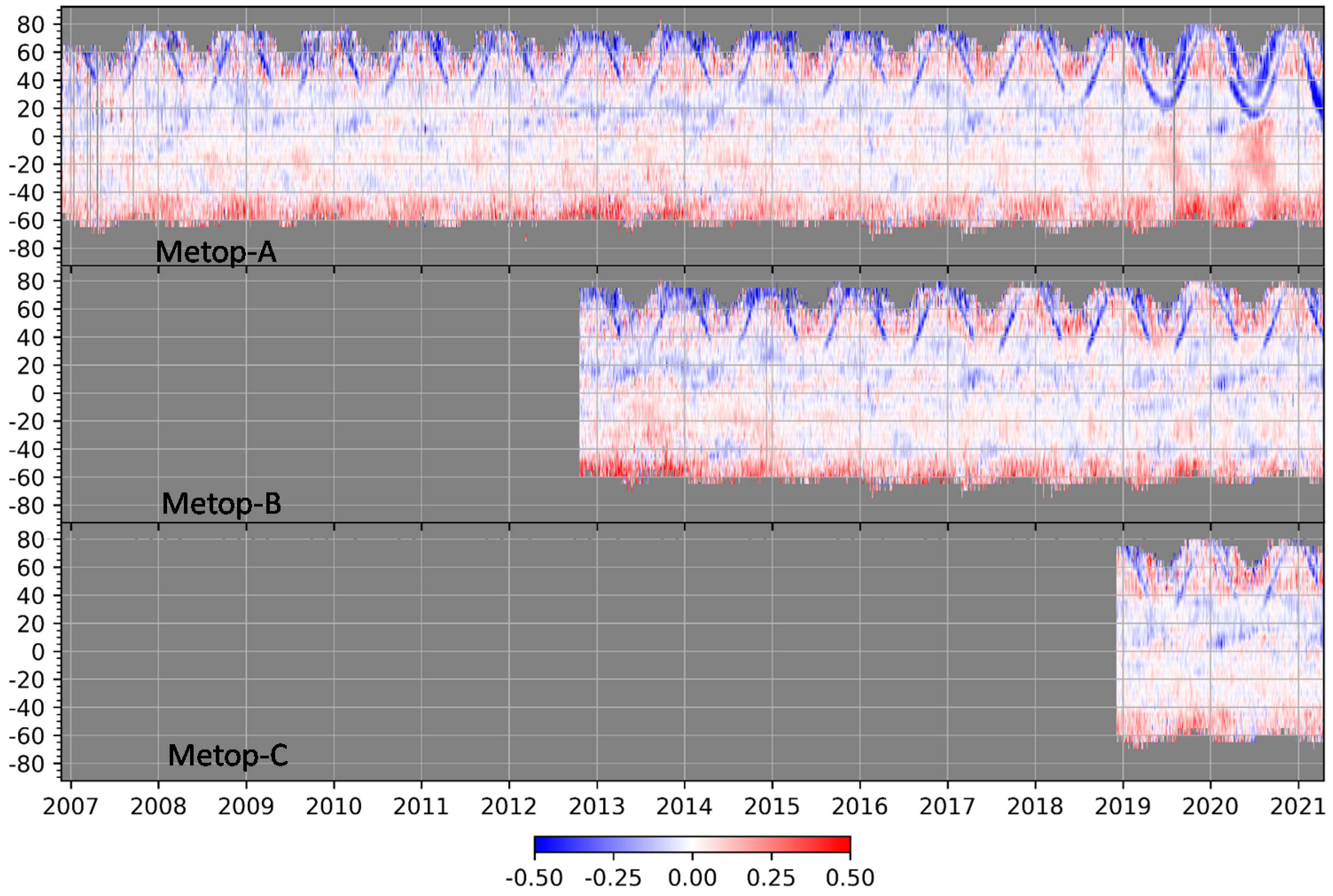
Figure 19 shows nighttime Hovmöller diagrams of GR—(D + TM) SST biases. All three products exhibit warm biases in the Southern Hemisphere (SH) high latitudes, reaching ~0.2–0.3 K, during the SH summers, and almost simultaneously, cold biases up to −0.2 K in the Northern Hemisphere (NH) high latitudes. Increased biases may be due to these high-latitude situations being under-represented in the training MDS, which requires extrapolation of the SST retrieval algorithm to situations not well covered by the global MDS. The second prominent feature of Figure 19 are the “cold arches” in the NH. They originate from the calibration errors caused by Sun impingement on the AVHRR black body calibration target, when the satellite orbit approaches the terminator from the dark side of the Earth. Note that this effect has intensified in Metop-A SST since 2019, approximately three years after its orbit ceased being controlled. More detailed (but still preliminary) discussions of this effect are found in [7].
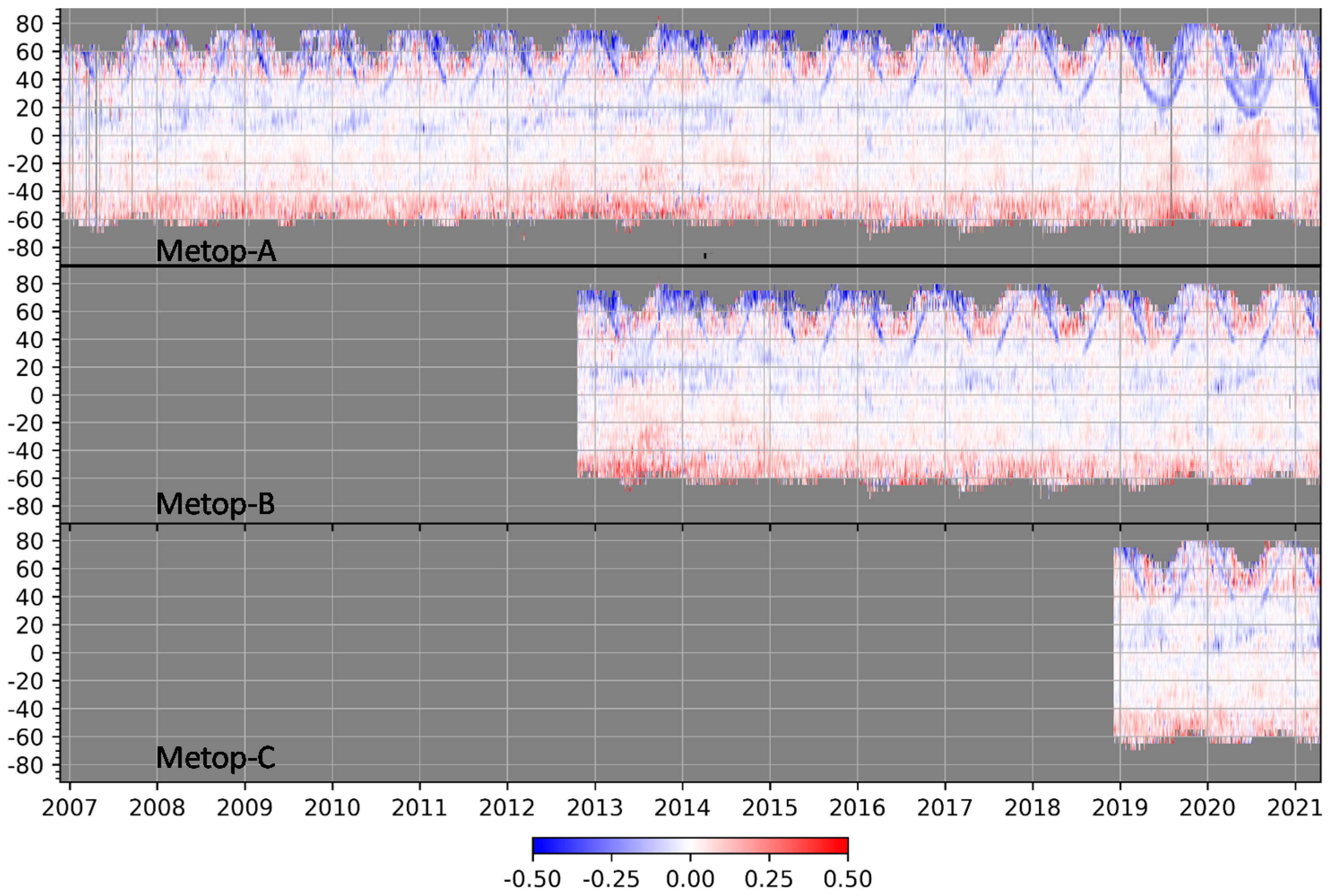
Figure 20 shows the latitudinal Hovmöller diagrams of nighttime PWR—(D + TM) SST biases. The high-latitude anomalies are reduced but not fully eliminated.
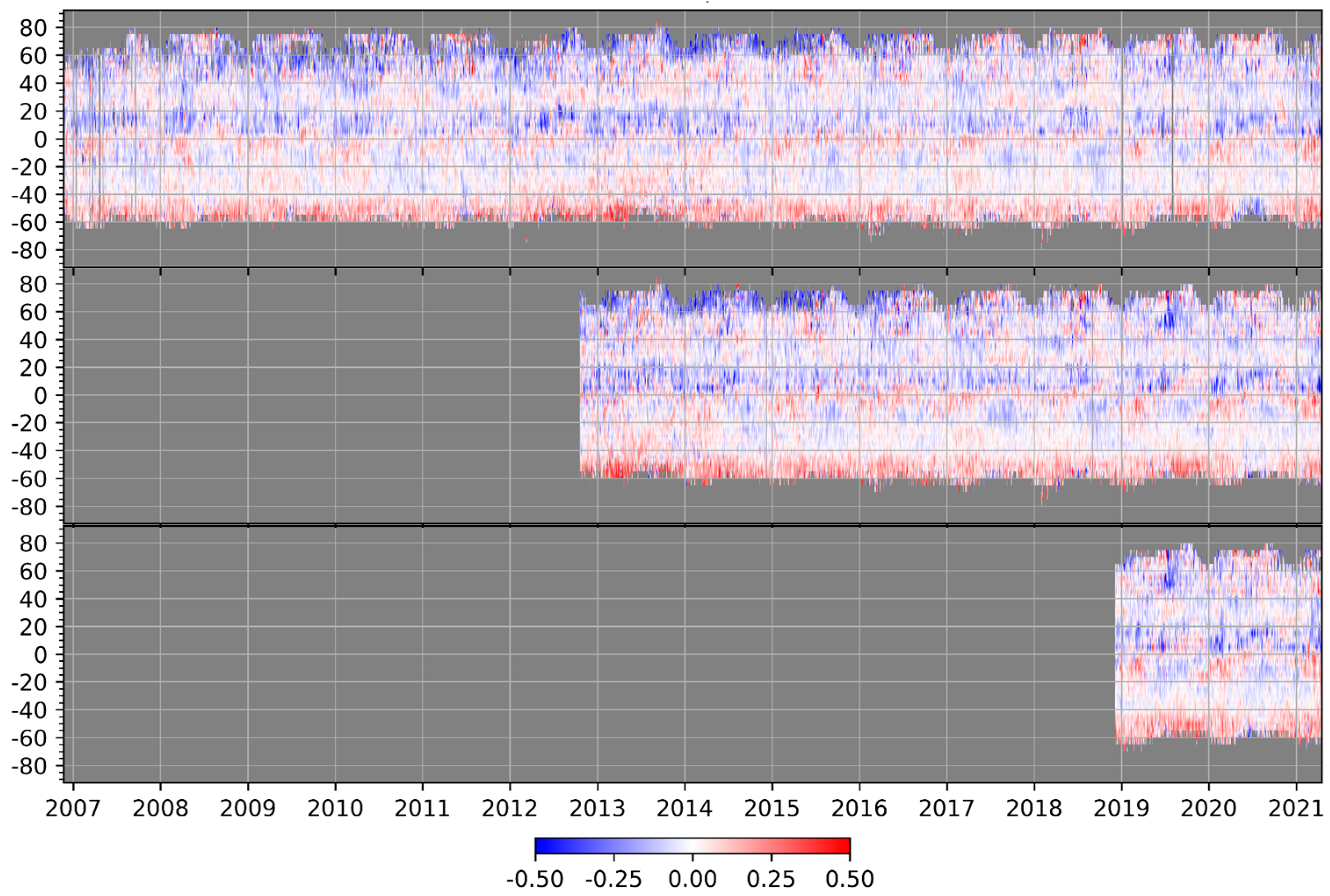
Figure 21 and Figure 22 show the daytime latitudinal Hovmöller diagrams for GR– (D + TM) and PWR– (D + TM) SSTs, respectively. The calibration artifacts are not seen in the daytime diagrams, but the warm biases in the Southern high and low latitudes are still present. Recall that these areas are under-represented in the corresponding MDS. The systematic cold biases in daytime SSTs are also noticeable in the 0°–20° N latitudinal band.
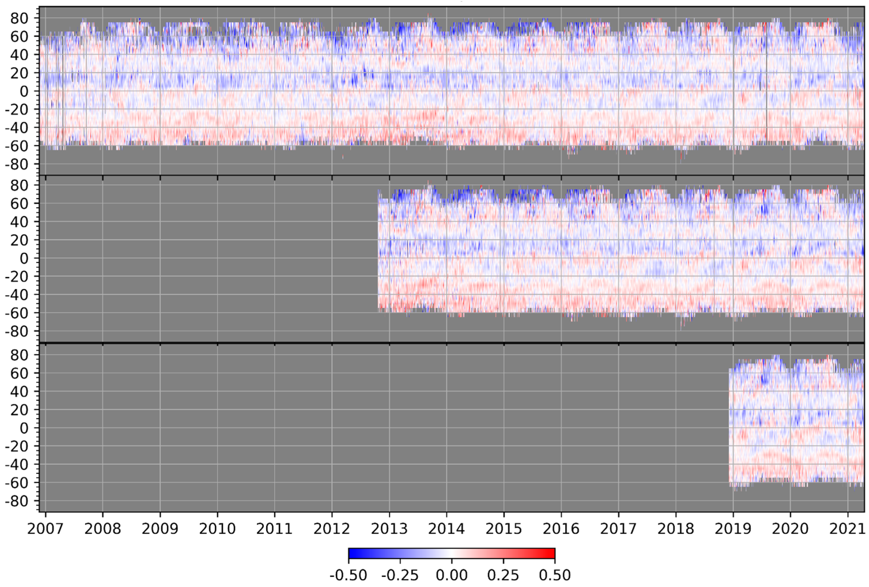
As for the nighttime anomalies, the daytime PWR shown in Figure 22 reduces the SST anomalies but does not eliminate them fully. This may require fine-tuning or revisiting the PWR and training algorithms, in the future AVHRR FRAC Reanalyses.
To summarize, high-latitude biases are seen in both GR and PWR SSTs. Those are due to a combination of the suboptimal AVHRR calibration on the current operational L1b data and limitations of the adopted SST equations, in conjunction with relatively sparse coverage of the near-polar regions with matchups. The GR in the high latitudes basically represents an extrapolation of the fitting the low-to-mid-latitudes matchups. The PWR SST does not mitigate these biases either (recall that the PWR coefficients are calculated only if a sufficient number of matchups is available within a given segment in the R-space; otherwise, the GR coefficients are used, which is often the case in the high-latitudes, where matchups are very sparse). Improved AVHRR calibration and SST algorithms will be explored in the next AVHRR FRAC Reanalysis, RAN2.
7. Thermal Fronts
The AVHRR FRAC RAN1 dataset was produced with ACSPO v2.80, which includes two new layers in the output files: ’sst_front_position’ and ‘sst_gradient_magnitude’, derived from the GR SST. The first layer represents a bit indicating the presence of the front in a given pixel. The second layer gives the magnitude of the front (NaN, if no front presence bit is set). Below we briefly illustrate the new ACSPO functionality, for interested users.
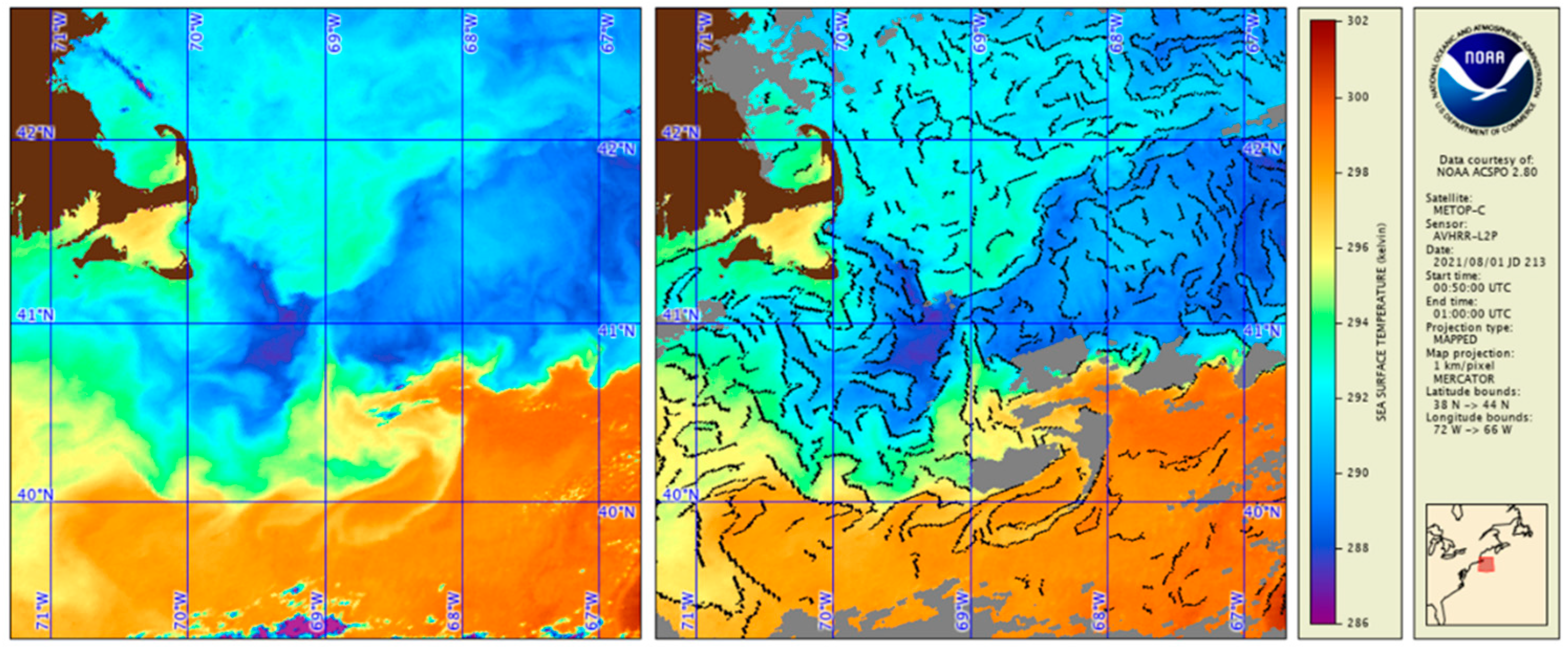
Figure 23 shows the nighttime GR SST over the Georges Bank/Nantucket Shoals on 1 August 2021, with and without ACSM and thermal fronts overlaid. Visually, the thermal fronts shown in the right panel, well capture the positions of SST gradients. Validation and documentation of this new ACSPO thermal fronts product is underway and will be reported elsewhere.
Another observation from Figure 23 is that the current ACSM performs reasonably well in the lower and upper parts of the image, whereas in the central area, it over-screens dynamic SST features. Even more over-screening may occur on some other days and/or areas (not shown). Oftentimes, if clouds are present in the scene, the current ACSM typically captures them quite well, but tends to over-screen, especially in coastal and dynamic areas. Work is underway to mitigate this overly conservative nature of the current ACSM.
8. Summary
The first complete and consistent global SST record from 1-km AVHRR FRAC data onboard three Metop-FG (Metop-A, -B and -C) was created with the NOAA Advanced Clear-Sky Processor for Ocean (ACSPO) version 2.80 SST system. The 1st historical reprocessing (Reanalysis-1, RAN1) goes back to the beginning of each satellite mission, and continues into near-real time (NRT). Special steps are taken to process NRT data maximally consistently with RAN, given the lack of the right-hand side of the time scale in real time operations. Improved science-quality RAN reprocessing follows the NRT processing, with a two-month lag.
Metop AVHRR FRAC BTs are more stable than in the NOAA AVHRR GAC data [2]. Nevertheless, they still suffer from residual instabilities on order of several tenths of a degree Kelvin. Those are mitigated by daily recalculation of regression coefficients against match-ups with iQuam Drifters and Tropical Moorings. In FRAC RAN1, the coefficients are calculated using matchups collected within time windows centered at the processed day. In NRT, the coefficients are derived from delayed windows of the same size ending from 4 to 10 days before the processed day. Anchoring satellite SSTs to (D + TM) reconciles satellite SSTs with in situ data, and across different platforms. It does not however affect the global SDs, which remain the same as in the data processed with fixed SST coefficients.
Independent validation against Argo floats confirms that derived SSTs are indeed stable in time and highly cross-platform consistent. Significantly sparser number of matchups, and deeper depths of AF measurements (~6 m), leads to noisier validation statistics, but the satellite SSTs continue meeting, and often exceeding with a wide margin, the NOAA specifications.
Additional consistency checks against CMC L4 SST (also fully independent of the Metop-FG RAN1) suggest that other than meeting the formal NOAA requirements, the newly created dataset is capable of supporting a wide variety of finer analyses and applications. In particular, for the first time it is demonstrated that a LEO product can successfully resolve a tiny diurnal SST signal between ~9:30 pm/am LT, a ~0.05 K cooling. Metop-A orbital degradation (to ~8 pm/am in August 2021) increases this diurnal signal to ~0.10 K.
Temporal anchoring of the ACSPO to (D + TM) SSTs reconciles satellite and in situ data. The ACSPO PWR SST (calculated in current ACSPO as GR SST minus SSES bias) further reduces the variability of global ACSPO minus in situ SST deltas. Moreover, the PWR SST reduces regional biases, thus improving the standard deviation of fitting in situ SSTs. Using the PWR SST, derived with variable regression coefficients, ensures using most stable time series, in conjunction with minimized regional biases.
Linking satellite SST to in situ SSTs has its merits and advantages, as confirmed by the evaluation of the newly produced AVHRR FRAC RAN1 dataset. By design, satellite SSTs are maximally reconciled with in situ data, at the stage of data production. Note that oftentimes, such satellite—in situ SST reconciliation is carried out by the L4 data producers, at the stage of assimilating satellite L2/3 data in their analyses. As a first step, they ‘bias-correct’ satellite SSTs and reconcile it with in situ SST. The FRAC RAN1 dataset meets users half way, in their desire of two maximally consistent data sets. L4 producers are still welcome to run their standard bias-correction (which however is expected to be of less value to the data assimilation, but this expectation must be independently tested and verified). The major challenge of the methodology relying on anchoring satellite SSTs to in situ data, is that one needs to ensure that the in situ dataset employed for such anchoring, is of high quality, globally representative (in terms of their spatial distribution), and stable and consistent in time. More analyses are needed to ensure that these conditions are indeed met, and no significant artifacts introduced in the satellite product, due to the evolving, not fully uniform and/or globally representative/fully optimal, in situ SST network. In that regard, the Metop-FG era from 2006-on is relatively rich with in situ data, compared to much more challenging earlier satellite years (1980–90s).
The new feature of the AVHRR FRAC data set is the availability of two additional layers, which characterize the positions and intensity of the ocean thermal fronts. This is a new product, derived and provided following numerous users’ requests. Its evaluation and documentation is still underway, as of this writing.
The ongoing next stage of the Metop FRAC SST Reanalysis is the mitigation of the AVHRR L1B calibration errors near the terminator, which causes cold biases in the northern hemisphere. Improvements to the ACSPO Clear-Sky Mask (to mitigate the overly conservative performance in the dynamic and coastal areas, and remaining cold biases in the highly cloudy and aerosol-contaminated areas), and to the SST retrieval, error characterization and training algorithms (to mitigate the remaining regional, including the high latitude warm biases) are also being explored. These and other improvements based on users’ feedback (as well as resulting from our own use of the individual sensor L3U data to produce super-collated L3S-LEO-AM product from 3 Metops [13]) will be explored in the next release of Metop-FG AVHRR FRAC RAN2, tentatively planned in 2024.
Author Contributions
Conceptualization, A.I.; methodology, B.P., V.P. and A.I.; software, Y.K., V.P. and B.P.; validation, V.P., B.P. and A.I.; formal analysis, V.P., B.P. and A.I.; investigation, A.I., V.P. and B.P.; resources, A.I.; data curation, B.P., V.P.; writing—original draft preparation, V.P., B.P.; writing—review and editing, A.I., V.P. and B.P.; visualization, V.P., B.P.; supervision, A.I.; project administration, A.I.; funding acquisition, A.I. All authors have read and agreed to the published version of the manuscript.
Funding
This research was funded by the NOAA Ocean Remote Sensing Program.
Institutional Review Board Statement
Not applicable.
Informed Consent Statement
Not applicable.
Data Availability Statement
Metop-FG SST products are available at NASA/JPL PO.DAAC https://podaac.jpl.nasa.gov/ (accessed on 25 August 2021) and NOAA NCEI https://www.ncei.noaa.gov/metadata/geoportal/ (accessed on 25 August 2021). Metop-FG Level 1b data have been provided courtesy of the NOAA STAR Central Data Repository managed by the STAR Data Management Working Group (Bob Kuligowski, Chair).
Acknowledgments
The authors acknowledge support of Wen-Hao Li, Edward Armstrong, and Tim McKnight of NASA/JPL PO.DAAC, and John Relph and Yongsheng Zhang of NOAA/NCEI with archival of the Metop-FG SST dataset. Thanks go to Olafur Jonasson and Irina Gladkova, NOAA STAR, for help with data processing and advice. The views, opinions, and findings in this report are those of the authors and should not be construed as an official NOAA or U.S. government position or policy.
Conflicts of Interest
The authors declare no conflict of interest.
References
- Petrenko, B.; Ignatov, A.; Kihai, Y.; Heidinger, A. Clear-Sky Mask for the Advanced Clear-Sky Processor for Oceans. J. Atmos. Ocean Tech. 2010, 27, 1609–1623. [Google Scholar] [CrossRef]
- Ignatov, A.; Zhou, X.J.; Petrenko, B.; Liang, X.M.; Kihai, Y.; Dash, P.; Stroup, J.; Sapper, J.; DiGiacomo, P. AVHRR GAC SST Reanalysis Version 1 (RAN1). Remote Sens. 2016, 8, 315. [Google Scholar] [CrossRef] [Green Version]
- Petrenko, B.; Ignatov, A.; Kihai, Y.; Dash, P. Sensor-Specific Error Statistics for SST in the Advanced Clear-Sky Processor for Oceans. J. Atmos. Ocean Tech. 2016, 33, 345–359. [Google Scholar] [CrossRef]
- Petrenko, B.; Ignatov, A.; Kihai, Y.; Stroup, J.; Dash, P. Evaluation and selection of SST regression algorithms for JPSS VIIRS. J. Geophys. Res.-Atmos. 2014, 119, 4580–4599. [Google Scholar] [CrossRef]
- Ignatov, A.; Gladkova, I.; Ding, Y.N.; Shahriar, F.; Kihai, Y.; Zhou, X.J. JPSS VIIRS level 3 uncollated sea surface temperature product at NOAA. J. Appl. Remote Sens. 2017, 11, 032405. [Google Scholar] [CrossRef]
- Pryamitsyn, V.; Petrenko, B.; Ignatov, A.; Jonasson, O.; Kihai, Y. Historical and near-real time SST retrievals from MetOp AVHRR FRAC with the advanced clear-sky processor for ocean. Ocean Sens. Monit. 2021, 13, 11752. [Google Scholar] [CrossRef]
- Petrenko, B.; Pryamitsyn, V.; Ignatov, A. Filtering cold outliers in SSTs retrieved from early AVHRRs for the second AVHRR GAC reanalysis. Ocean. Sens. Monit. 2021, 13, 11752. [Google Scholar] [CrossRef]
- Pryamitsyn, V.; Ignatov, A.; Petrenko, B.; Jonasson, O.; Kihai, Y. Evaluation of the initial NOAA AVHRR GAC SST Reanalysis Version 2 (RAN2 B01). Proc. Spie 2020, 11420. [Google Scholar] [CrossRef]
- Plans for Metop-A End of Life. Available online: https://www.eumetsat.int/plans-metop-end-life (accessed on 23 April 2021).
- Metop Second Generation. Available online: https://www.nesdis.noaa.gov/OPPA/metop-sg.php (accessed on 19 August 2021).
- Jonasson, O.; Ignatov, A. Status of second VIIRS reanalysis (RAN2). SPIE Def. Commer. Sens. 2019, 11014, 1101400. [Google Scholar] [CrossRef]
- Jonasson, O.; Gladkova, I.; Ignatov, A.; Kihai, Y. Progress with Development of Global Gridded Super-Collated SST Products from Low Earth Orbiting Satellites (L3S-LEO) at NOAA; SPIE: Bellingham, MA, USA, 2020; Volume 11420. [Google Scholar]
- Jonasson, O.; Gladkova, I.; Ignatov, A.; Kihai, Y. Algorithmic Improvements and Consistency Checks of the NOAA Global Gridded Super-Collated SSTs from Low Earth Orbiting Satellites (ACSPO* L3S-LEO); SPIE: Bellingham, MA, USA, 2021; Volume 11752. [Google Scholar]
- STAR. GHRSST NOAA/STAR Metop-A AVHRR FRAC ACSPO v2.80 0.02º L3U Dataset (GDS v2); Jet Propulsion Laboratory: Pasadena, CA, USA, 2021. [CrossRef]
- STAR. GHRSST NOAA/STAR Metop-A AVHRR FRAC ACSPO v2.80 1 km L2P Dataset (GDS v2); Jet Propulsion Laboratory: Pasadena, CA, USA, 2021. [CrossRef]
- STAR. GHRSST NOAA/STAR Metop-B AVHRR FRAC ACSPO v2.80 0.02º L3U Dataset (GDS v2); Jet Propulsion Laboratory: Pasadena, CA, USA, 2021. [CrossRef]
- STAR. GHRSST NOAA/STAR Metop-B AVHRR FRAC ACSPO v2.80 1 km L2P Dataset (GDS v2); Jet Propulsion Laboratory: Pasadena, CA, USA, 2021. [CrossRef]
- STAR. GHRSST NOAA/STAR Metop-C AVHRR FRAC ACSPO v2.80 0.02º L3U Dataset (GDS v2); Jet Propulsion Laboratory: Pasadena, CA, USA, 2021. [CrossRef]
- STAR. GHRSST NOAA/STAR Metop-C AVHRR FRAC ACSPO v2.80 1 km L2P Dataset (GDS v2); Jet Propulsion Laboratory: Pasadena, CA, USA, 2021. [CrossRef]
- OSI SAF. GHRSST Level 2P Sub-Skin Sea Surface Temperature from the Advanced Very High Resolution Radiometer (AVHRR) on Metop Satellites (Currently Metop-A) (GDS V2) Produced by OSI SAF; OSI SAF: Hawthorne, CA, USA, 2015. [Google Scholar] [CrossRef]
- OSI SAF. GHRSST Level 2P Global Subskin Sea Surface Temperature from the Advanced Very High Resolution Radiometer (AVHRR) on the MetOp-B Satellite (GDS2 Version); OSI SAF: Hawthorne, CA, USA, 2016. [Google Scholar] [CrossRef]
- Dash, P.; Ignatov, A.; Kihai, Y.; Sapper, J. The SST Quality Monitor (SQUAM). J. Atmos. Ocean. Tech. 2010, 27, 1899–1917. [Google Scholar] [CrossRef]
- SST Quality Monitor (SQUAM AVHRR FRAC). Available online: https://www.star.nesdis.noaa.gov/socd/sst/squam/polar/avhrrfrac/ (accessed on 30 April 2021).
- Xu, F.; Ignatov, A. In situ SST Quality Monitor (iQuam). J. Atmos. Ocean Tech. 2014, 31, 164–180. [Google Scholar] [CrossRef]
- In Situ SST Quality Monitor System (iQuam). Available online: https://www.star.nesdis.noaa.gov/socd/sst/iquam/ (accessed on 30 April 2021).
- Petrenko, B.; Pryamitsyn, V.; Ignatov, A.; Kihai, Y. SST and Cloud Mask Algorithms in Reprocessing 1981–2002 NOAA AVHRR Data for SST with the Advanced Clear-Sky Processor for Oceans (ACSPO); SPIE: Bellingham, MA, USA, 2020; Volume 11420. [Google Scholar]
- ACSPO Regional Monitor for SST v2.1 (ARMS). Available online: https://www.star.nesdis.noaa.gov/socd/sst/arms/ (accessed on 1 June 2021).
- Marsouin, A.; Le Borgne, P.; Legendre, G.; Pere, S.; Roquet, H. Six years of OSI-SAF METOP-A AVHRR sea surface temperature. Remote Sens. Environ. 2015, 159, 288–306. [Google Scholar] [CrossRef]
- Kilpatrick, K.A.; Podesta, G.P.; Evans, R. Overview of the NOAA/NASA advanced very high resolution radiometer Pathfinder algorithm for sea surface temperature and associated matchup database. J. Geophys. Res.-Oceans 2001, 106, 9179–9197. [Google Scholar] [CrossRef]
- Brasnett, B.; Colan, D.S. Assimilating Retrievals of Sea Surface Temperature from VIIRS and AMSR2. J. Atmos. Ocean Tech. 2016, 33, 361–375. [Google Scholar] [CrossRef]
- Petrenko, B.; Ignatov, A.; Kramar, M.; Kihai, Y. Exploring New Bands in Modified Multichannel Regression SST Algorithms for the Next-Generation Infrared Sensors at NOAA; SPIE: Bellingham, MA, USA, 2016; Volume 9827. [Google Scholar]
- Walton, C.C.; Pichel, W.G.; Sapper, J.F.; May, D.A. The development and operational application of nonlinear algorithms for the measurement of sea surface temperatures with the NOAA polar-orbiting environmental satellites. J. Geophys Res.-Oceans 1998, 103, 27999–28012. [Google Scholar] [CrossRef]
- Merchant, C.J.; Harris, A.R.; Roquet, H.; Le Borgne, P. Retrieval characteristics of non-linear sea surface temperature from the Advanced Very High Resolution Radiometer. Geophys. Res. Lett. 2009, 36. [Google Scholar] [CrossRef] [Green Version]
- MICROS 2. Monitoring of IR Clear-Sky Radiances over Oceans for SST. Available online: https://www.star.nesdis.noaa.gov/socd/sst/micros/ (accessed on 31 May 2021).
- Visible/IR Spectral Response Functions (SRFs) and MW Passbands. Available online: https://www.nwpsaf.eu/site/software/rttov/download/coefficients/spectral-response-functions/ (accessed on 30 April 2021).
- Ignatov, A.; Laszlo, I.; Harrod, E.D.; Kidwell, K.B.; Goodrum, G.P. Equator crossing times for NOAA, ERS and EOS sun-synchronous satellites. Int. J. Remote Sens. 2004, 25, 5255–5266. [Google Scholar] [CrossRef]
- He, K.; Ignatov, A.; Kihai, Y.; Cao, C.Y.; Stroup, J. Sensor Stability for SST (3S): Toward Improved Long-Term Characterization of AVHRR Thermal Bands. Remote Sens. 2016, 8, 346. [Google Scholar] [CrossRef] [Green Version]
- 3S Sensor Stability for SST v2.0. Available online: https://www.star.nesdis.noaa.gov/socd/sst/3s/ (accessed on 30 April 2021).
- Liang, X.M.; Ignatov, A.; Kihai, Y. Implementation of the Community Radiative Transfer Model in Advanced Clear-Sky Processor for Oceans and validation against nighttime AVHRR radiances. J. Geophys. Res.-Atmos. 2009, 114. [Google Scholar] [CrossRef]
- Liang, X.; Ignatov, A. Monitoring of IR Clear-Sky Radiances over Oceans for SST (MICROS). J. Atmos. Ocean Tech. 2011, 28, 1228–1242. [Google Scholar] [CrossRef] [Green Version]
Figure 1.
Spectral response functions (SRFs) of the (red) Metop-A, (green) Metop-B, and (blue) Metop-C in AVHRR thermal bands (left) 3b, (center) 4, and (right) 5 [35].
Figure 1.
Spectral response functions (SRFs) of the (red) Metop-A, (green) Metop-B, and (blue) Metop-C in AVHRR thermal bands (left) 3b, (center) 4, and (right) 5 [35].

Figure 2.
Local equator crossing times (LEXT) for Metop-A/B/C and NOAA-18/19. (From the NOAA Sensor Stability for SST, 3S system [37,38] which calculates the LEXTs following [36].).

Figure 3.
Orbital average (over nighttime part of the orbit) calibration gains in AVHRR/3 channel 3B for Metop-A/B/C and NOAA-18/19. (From the NOAA Sensor Stability for SST, 3S system [37,38]).

Figure 4.
Monthly aggregated Observation—Model (O-M) biases in AVHRR thermal bands (top) 3.7 µm; (middle) 11 µm; (bottom) 12 µm of three Metop-FG satellites: (left) night; (right) day. Data are from the NOAA MICROS system [34,40].

Figure 5.
Monthly aggregated GR—(D + TM) SST biases computed with static regression coefficients: (left): night; (right) day.
Figure 5.
Monthly aggregated GR—(D + TM) SST biases computed with static regression coefficients: (left): night; (right) day.

Figure 6.
Nighttime yearly aggregated maps of Metop-B GR—in situ SSTs in 2016, for two in situ references: (left) D + TM; (right) AF.
Figure 6.
Nighttime yearly aggregated maps of Metop-B GR—in situ SSTs in 2016, for two in situ references: (left) D + TM; (right) AF.

Figure 7.
Time series of the monthly aggregated number of observations in the MDSs: (top) night; (bottom) day vs. (left) (D + TM); (right) AF.
Figure 7.
Time series of the monthly aggregated number of observations in the MDSs: (top) night; (bottom) day vs. (left) (D + TM); (right) AF.

Figure 8.
Yearly aggregated histograms of ACSPO—(D + TM) SST for Metop-B in 2016. (Left) night; (right) day; (top) GR; (bottom) PWR.
Figure 8.
Yearly aggregated histograms of ACSPO—(D + TM) SST for Metop-B in 2016. (Left) night; (right) day; (top) GR; (bottom) PWR.

Figure 9.
Time series of 24-h aggregated ACSPO—(D + TM) SST global mean biases. (Top) night; (bottom) day; (left) GR; (right) PWR.
Figure 9.
Time series of 24-h aggregated ACSPO—(D + TM) SST global mean biases. (Top) night; (bottom) day; (left) GR; (right) PWR.

Figure 10.
Same as in Figure 9 but for the global standard deviations (SD).
Figure 10.
Same as in Figure 9 but for the global standard deviations (SD).

Figure 11.
Same as in Figure 8 but against AFs.
Figure 11.
Same as in Figure 8 but against AFs.

Figure 12.
Time series of monthly ACSPO—AF SST global mean biases. (Top) night; (bottom) day; (left) GR; (right) PWR.
Figure 12.
Time series of monthly ACSPO—AF SST global mean biases. (Top) night; (bottom) day; (left) GR; (right) PWR.

Figure 13.
Same as in Figure 12, but for the global standard deviations (SDs).
Figure 13.
Same as in Figure 12, but for the global standard deviations (SDs).

Figure 14.
Yearly composite maps of Metop-B ACSPO—L4 CMC SST in 2016. (Top) night; (bottom) day; (left) GR; (right) PWR.
Figure 14.
Yearly composite maps of Metop-B ACSPO—L4 CMC SST in 2016. (Top) night; (bottom) day; (left) GR; (right) PWR.

Figure 15.
Time series of global ACSPO—L4 CMC SST mean biases. (Top) night; (bottom) day; (left) GR; (right) PWR.
Figure 15.
Time series of global ACSPO—L4 CMC SST mean biases. (Top) night; (bottom) day; (left) GR; (right) PWR.

Figure 16.
Time series of global monthly aggregated (day ACSPO—L4 CMC) minus (night ACSPO—L4 CMC) SST Double Differences. (Left) GR; (right) PWR.
Figure 16.
Time series of global monthly aggregated (day ACSPO—L4 CMC) minus (night ACSPO—L4 CMC) SST Double Differences. (Left) GR; (right) PWR.

Figure 17.
Same as in Figure 15 but for the corresponding global standard deviations (SDs).
Figure 17.
Same as in Figure 15 but for the corresponding global standard deviations (SDs).

Figure 18.
Time series of 24 h aggregated (left) night and (right) day clear-sky fractions (in %).

Figure 19.
Hovmöller diagrams of 24 h aggregated latitudinal biases in nighttime GR—(D + TM) SST for the full Metop-FG missions.
Figure 19.
Hovmöller diagrams of 24 h aggregated latitudinal biases in nighttime GR—(D + TM) SST for the full Metop-FG missions.

Figure 20.
Same as in Figure 19 but for nighttime PWR—(D + TM) SST.
Figure 20.
Same as in Figure 19 but for nighttime PWR—(D + TM) SST.

Figure 21.
Same as in Figure 19 but for daytime GR—(D + TM) SST.
Figure 21.
Same as in Figure 19 but for daytime GR—(D + TM) SST.

Figure 22.
Same as in Figure 19 but for daytime PWR—(D + TM) SST.
Figure 22.
Same as in Figure 19 but for daytime PWR—(D + TM) SST.

Figure 23.
Nighttime maps of GR SST in the Georges Bank/Nantucket Shoals on 1 August 2021. The left map is an ‘all-sky’ SST, the right map applies the ACSPO Clear-Sky Mask (ACSM; rendered in grey) and overlays thermal fronts (in black lines). Maps are taken from the NOAA ACSPO Regional Monitor for SST system (ARMS) [27]. Land is rendered in dark brown.

Publisher’s Note: MDPI stays neutral with regard to jurisdictional claims in published maps and institutional affiliations. |
© 2021 by the authors. Licensee MDPI, Basel, Switzerland. This article is an open access article distributed under the terms and conditions of the Creative Commons Attribution (CC BY) license (https://creativecommons.org/licenses/by/4.0/).
Share and Cite
MDPI and ACS Style
Pryamitsyn, V.; Petrenko, B.; Ignatov, A.; Kihai, Y. Metop First Generation AVHRR FRAC SST Reanalysis Version 1. Remote Sens. 2021, 13, 4046. https://0-doi-org.brum.beds.ac.uk/10.3390/rs13204046
AMA Style
Pryamitsyn V, Petrenko B, Ignatov A, Kihai Y. Metop First Generation AVHRR FRAC SST Reanalysis Version 1. Remote Sensing. 2021; 13(20):4046. https://0-doi-org.brum.beds.ac.uk/10.3390/rs13204046
Chicago/Turabian StylePryamitsyn, Victor, Boris Petrenko, Alexander Ignatov, and Yury Kihai. 2021. "Metop First Generation AVHRR FRAC SST Reanalysis Version 1" Remote Sensing 13, no. 20: 4046. https://0-doi-org.brum.beds.ac.uk/10.3390/rs13204046
Note that from the first issue of 2016, this journal uses article numbers instead of page numbers. See further details here.