Article

Shallow Water Bathymetry Retrieval Using a Band-Optimization Iterative Approach: Application to New Caledonia Coral Reef Lagoons Using Sentinel-2 Data

1
Institut Français de Recherche pour l’Exploitation de la MER, UMR 9220 ENTROPIE (Institut de Recherche pour le Développement, Université de la Réunion, IFREMER, Centre National de la Recherche Scientifique, Université de la Nouvelle-Calédonie), BP 32078, 98848 Nouméa, New Caledonia, France
2
Institut de Recherche pour le Développement, UMR 9220 ENTROPIE (IRD, IFREMER, Université de la Réunion, Centre National de la Recherche Scientifique, Université de la Nouvelle-Calédonie), BP A5, 98848 Nouméa, New Caledonia, France
*
Author to whom correspondence should be addressed.
Remote Sens. 2021, 13(20), 4108; https://0-doi-org.brum.beds.ac.uk/10.3390/rs13204108
Submission received: 15 September 2021 / Revised: 8 October 2021 / Accepted: 11 October 2021 / Published: 14 October 2021
(This article belongs to the Special Issue Remote Sensing of the Aquatic Environments-Part II)

Abstract

:
To achieve high accuracy bathymetry retrieval using remote sensing images with robust performance in a 0 to 25 m-deep lagoon with sharp bottom depth variations, a new Iterative Multiple Band Ratio (IMBR) algorithm is tested against known Multiple Band Ratio (MBR) and Single Band Ratio (SBR) algorithms. The test was conducted using the five multispectral bands, at 10 to 60 m resolution, of a Sentinel-2 image of the 25 km2 Poe lagoon, a UNESCO World Heritage Area. The IMBR approach requires training datasets for the definitions of depth threshold at which optimal band ratios vary. IMBR achieved accuracy, quantified with an original block cross-validation procedure across the entire depth range reached a mean absolute error of 46.0 cm. It compares very favorably against MBR (78.3 cm) and the various SBR results (188–254 cm). The method is suitable for generalization to other sites pending a minimal ground-truth dataset crossing all the depth range being available. We stress that different users may need different precisions and can use MBR or SBR algorithms for their applications. For the hydrodynamic modelling applications that are developing in New Caledonia, the IMBR solutions applied to Sentinel imagery are optimal.

1. Introduction

Knowledge of bathymetry is a critical issue for many coastal scientific and management applications. In shallow coral reefs and lagoons, bathymetry plays an important role in geophysical and biological processes: living communities, substrate types and habitat zonation are frequently related to water depth [1], sedimentary facies are controlled by depth and energy regime [2,3] and coral bleaching is also depth-dependent [4]. In terms of applied coastal studies, accurate bathymetry is paramount to achieve many applications, from the assessment of coasts facing storms or changing climate conditions [5], to realistic hydrodynamic 3D modelling [6,7] or the exploration of submerged landscapes and archaeological sites [8,9].
In New Caledonia, located in the Southwest Pacific, sediments produced in particular by the mining industry impact marine living communities all around the main island, called Grande-Terre [10]. Hydrodynamic models are used to investigate the dynamics and fate of terrestrial inputs into the lagoons [11]. However, bathymetry is not known precisely everywhere for the 19,385 km2 of shallow and deep lagoons [12] that surround Grande-Terre. Gaps in bathymetric data have impaired the development of coastal models in the past, but recent projects aim to expand the current spatial coverage of hydrodynamic models from the south-west lagoon [11] to all lagoons around Grande-Terre. Therefore, it was necessary to investigate a relatively low-cost, fast, and accurate way to fill bathymetric gaps especially for shallow lagoon areas that cannot be navigated and surveyed with traditional hydrographic means using depth sounders.
Traditional bathymetric measurements made by echo-sounders, either single- or multi-beam, record water depth from the sea surface from some sort of sea-going vessels. This acquisition process remains expensive and time-consuming [13]. Furthermore, soundings in shallow water require specific compact echosounders which still cannot perform in the shallowest part of lagoons (0–1 m), out of reach even for small vessels. The problem is even more acute in areas with sharp bottom depth variations (i.e., rugose areas), such as around reticulated patch reefs that can be very extensive and impenetrable. Methods relying on airborne bathymetric LIDAR (Light Detection And Ranging) provide very efficient solutions in such shallow waters down to 30 m in clear waters, but remain very expensive despite improving in cost/coverage ratios [14,15]. Finally, satellite imagery can be interpreted to infer bathymetry synoptically using optical data with a wide range of spatial resolutions (from 300 m down to 1 m) and therefore at a much lower cost. However, the spatial resolution remains much lower than traditional hydroacoustic methods (~0.05 m).
Limitations of satellite optical imagery for bathymetric modelling have been extensively discussed in the past [16,17] and these inherent limits are still present today [18]. Nevertheless, developments are still on-going, taking advantage in particular of new multispectral high spatial resolution (1–10 m) sensors that allow new algorithms to be tested [19,20,21,22,23,24,25,26,27,28]. Specifically, for New Caledonia, a first attempt of bathymetry retrieval using MEdium Resolution Imaging Spectrometer (MERIS) scenes has been undertaken [29] but the spatial resolution was too coarse to be relevant for the development of numerical models. However, many of these recent developments use commercial imagery with narrow swath, whose processing would be too costly to cover all New Caledonia lagoons. Considering our constraints, we aimed for deriving Satellite-Derived Bathymetry (SDB) using preferentially the free wide-swath Sentinel-2 multispectral images. With a five-day revisit time, a 10 m medium-scale native resolution and its suitable spectral resolution, the European Space Agency sensor have high potential for marine and coastal applications [30,31,32,33,34], and its use for bathymetry retrievals is increasing [21,22,23,24].
Several methods relating to passive SDB have been demonstrated in recent years. These approaches can be subdivided into three different categories. The first category, based on empirical modelling, is the most commonly applied on passive hyperspectral and multispectral data [13]. These methods rely on a simple radiative model describing the subsurface water reflectance following depth [35,36,37,38], for instance
R ( h ) = r v ( 1 e α h ) + r b e α h
where h is the depth, r v is the reflectance due to volume scattering resulting from an infinitely deep-water column, r b is the bottom reflectance and α is a water attenuation coefficient considering downwelling and upwelling pathway. We follow here the notations and formalism provided by Lyzenga et al. [36].
Many complex processes and especially the air–water interface effects are often neglected, which allows the model form to be applied with reflectance as well as with radiance, most often assuming homogeneous effects of the atmosphere over the study area, which is generally small. As a result, three main factors of variation of the radiative signal are generally taken into account: water attenuation, bottom reflectance and volume scattering. Equations are solved by empirical estimation requiring in situ depth measurements or some simplifying hypotheses to remove some of the unknowns. These methods generally suffer from the natural spatial variability of water attenuation and bottom reflectance that are inherently overlooked, especially over large areas. For this reason, they are commonly applied by spatial regions after some sort of spatial segmentation is performed to limit the intra-region variability [39,40] and with locally tuned parameters [41,42].
The second category of satellite-derived bathymetric approaches regroups the so-called semi-analytic methods. These methods theoretically do not require in situ depth measurements. They consist of solving a more constrained equation system from the radiative transfer theory with more optically important parameters (Inherent Optical Properties, IOPs), but also with more control of the model error on water leaving reflectance retrievals [14]. Their advantages are that they provide a per pixel solution whose performances are spatially more stable than empirical methods and allow in parallel the evaluation of several optically important biophysical parameters such as chlorophyll concentration or backscattering coefficient. On the other hand, they require a spectral library of the so-called end-members and rely on the spectral matching between the simulated and the measured signals. An important first step is thus an accurate atmospheric correction. Considering the more complex equations and numbers of unknown factors to solve, these methods are more suitable for hyperspectral sensors [14,21,25].
Finally, the last category of bathymetric approaches regroups pure statistical classification or machine-learning methods. Most machine-learning processes targeting water depth retrieval rely on decision trees [43] or neural networks [44,45]. They are very efficient and accurate, but often require a large set of calibration measurements, in order to avoid over-fitting and to be able to generalize from one area to another. Neural networks present the advantages of considering the non-linear relationship that can occur between depth and optical signals [44].
This study describes the application of a new SDB algorithm based on Sentinel-2 data available from the Copernicus Program and its portal. The shallow and rugose Poe lagoon located on the west coast of New Caledonia is investigated, also using adequate ground-truthing for model calibration and validation. Specifically, after a brief review of the current state of the art, we evaluate the performance of single-band ratio and multi-band ratios models applied to Sentinel-2 data. We first applied these models to the shallowest part of the Poe lagoon (< 4 m) and then to an extended area including bathymetry up to 25 m. However, choosing suitable bands remains a difficult task and often results in depth-dependent performances, enabling good accuracy for either shallow or deep waters, but not both. To overcome this issue, a new band optimization iterative approach is proposed that optimally suited our objectives to perform well on shallow water lagoons displaying large and sharp bathymetric changes as well as very irregular shallow coral reef areas.

2. Materials and Methods
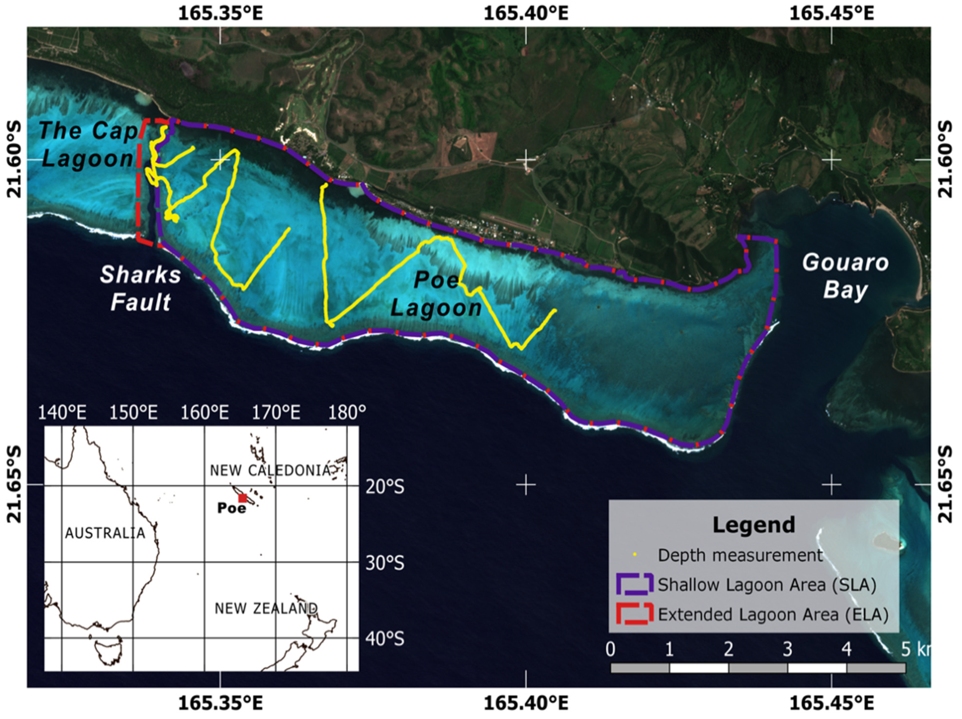
2.1. Study Site

The study site, the Poe area, is located in the central part of the west coast of New Caledonia. It is part of the UNESCO’s World Heritage Lagoons of New Caledonia. It includes a 25 km2 shallow sedimentary lagoon bounded on the shore side by an extensive seagrass bed. This shallow lagoon, quasi rectangular-shaped, is bounded on its western side by a narrow pass called the Sharks’ Fault (Faille aux Requins), and on its eastern side by the Gouaro Bay which is open onto the ocean. Finally, on the southern side, Poe lagoon is delimited by a 15 km long barrier reef (Figure 1). The lagoon itself contains several benthoscapes (e.g., bottom types, substrates, depth variability) such as sand, very low-density seagrass and algal beds, irregular coral structures and mixed hardground bottoms, which are more abundant eastward. With a maximum measured depth of about 25 m in the pass and a maximum depth of only 4 m in the inner lagoon, the study site demands a bathymetry retrieval process that is accurate for the narrow range of shallow depth found throughout most of the lagoon, while still being accurate within the 0–25 m range around the pass area. These constraints are, however, actually fairly typical of most island shallow reef systems, bordered by deep channels and slopes. Considering this, we hereafter defined two areas of interest for the rest of the study (Figure 1). The first one, called the Shallow Lagoon Area (SLA), encompasses only the inner lagoon whose maximum depth is less than 4 m. The second zone is then called the Extended Lagoon Area (ELA) and is composed of the SLA, the Sharks Fault and the eastern border of the Cap lagoon.

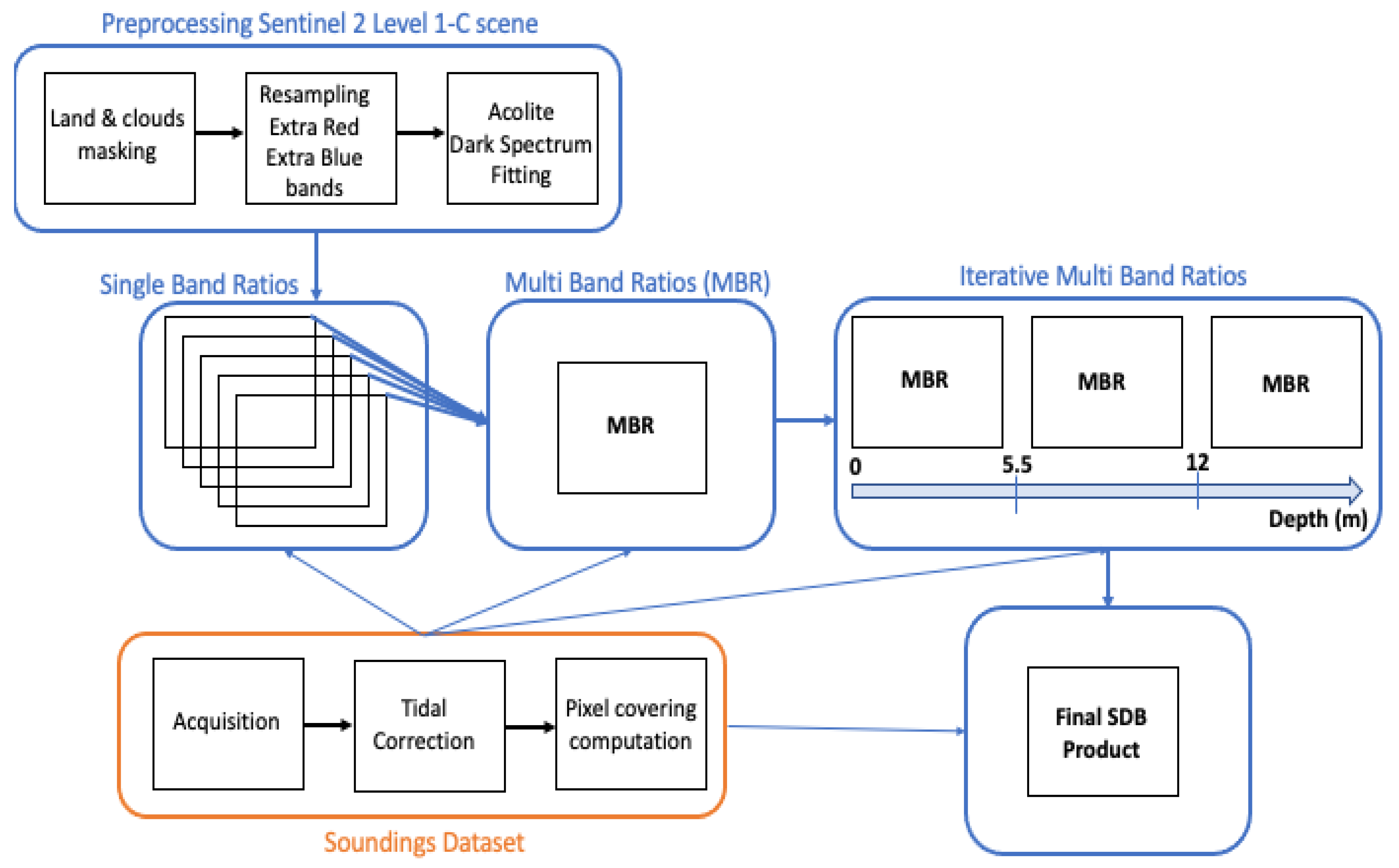
2.2. Sentinel-2 Imagery and Pre-Processing

The 10 m spatial resolution available for several bands of the MultiSpectral Instrument (MSI) Sentinel-2A and -2B sensors was deemed a good compromise to capture the topography of the area with adequate precision while allowing us to collect a reasonable amount of calibration/validation bathymetric data at the same resolution.
The open-data Sentinel-2 distribution strategy allows accessing numerous images, which is a significant advantage as different images can provide different qualities due to sea surface effect and glint, cloud cover or water clarity, which ultimately can alter any algorithm performances [22]. The choice of the ‘best’ image must follow several criteria. Ideally, the image should be free of apparent sea surface sunglint and with no cloud cover. Moreover, the end of high tide at the time of acquisition and low precipitation the days before the acquisition generally mean better water clarity and transparency for this area. The Sentinel-2A level 1-C image selected for this study (S2A_MSIL1C_20180305T230901) was captured on 5 March 2018, with a tide level of 1.31 m. Without any apparent glint in the lagoon that could have required some radiometric corrections [46], the image has been judged of sufficient quality.
Following the same philosophy than Kerr and Purkis [25], the five most water-penetrating spectral bands were considered (Table 1).
The land and few clouds were masked by thresholding the near-infrared band. Cloud cover was less than 1.5% with residual cloud shadows far away from the study site.
The shorter blue and longer red bands (Table 1) were resampled (nearest-neighbor method) at a spatial ground resolution of 10 m to match the higher spatial resolution of the other bands.
The image was atmospherically corrected using the ACOLITE software [47], which is designed to process Sentinel-2 and Landsat 5/7/8 for coastal and inland water application [48]. The method uses multiple dark targets in the scene to construct a “dark spectrum”, which is used to estimate the atmospheric path reflectance according to the best fitting aerosol model [28,49,50].

2.3. In Situ Acquisition and Processing

Empirical methods require depth datasets for training and validation purposes. This is compulsory for the calibration of the algorithms, and for accuracy assessment. In situ bathymetric transects were acquired using a single-beam echosounder in the deep pass (Sharks Fault) and in the shallow lagoon using a Seafloor HydroLite™-TM, HydroLite-DFX, which has a precision of 0.1% of actual depth (Figure 1). Records were georeferenced using a Geode, Juniper SystemTM, GPS. This campaign took place 22nd–23rd of May 2018. The survey was accomplished at a rate of 2 Hz with a maximum cruising speed of about 2 m/s. Records were resampled to provide approximately one sounding every 2 m. Finally, a pressure sensor was simultaneously deployed in the Poe lagoon to perform accurate tidal correction and to be in line with the chart datum of the Hydrographic Service of the French Navy.
In coral rugose environments, significant depth variation, even at a 10 m spatial resolution, within 100 m2-pixel can be found. In that case, insufficient coverage of in situ measurements can bias accuracy assessment since it is difficult to ascertain if a handful of in situ depth records can represent well the depth across the entire pixel. In order to reduce this bias in training or control, pixels overlapped by too few bathymetric records were discarded. For that purpose, a minimum threshold of 20% of pixel area covered by ground-truth data was applied. For valid pixels, the assigned ground-truth depth was the average of the overlapping in situ bathymetric records. Eventually, 607 pixels were kept, including 86 located within the Sharks Fault.

2.4. Baseline: The Stumpf Model with a Single Band-Ratio as an Enhancement of Empirical Models

Among the aforementioned first type of approaches (empirical modelling) and in order to reduce the effect of bottom reflectance changes, Stumpf et al. [38] proposed an empirical model based on the ratio of the logarithms of two bands i and j (practically blue and green), which can be expressed as
h ^ = m 1 ln ( n R w ( λ i ) ) ln ( n R w ( λ j ) ) m 0
where h ^ is the estimated depth, R w ( λ i )   the water reflectance for the spectral band i,   m 1 a tunable constant to scale the ratio to depth, m 0 an offset coefficient and n a fixed constant. In practice, it consists of calibrating two constants using in situ depth soundings: the scaling coefficient m 1 , and the offset coefficient m 0 . The constant n is only aimed at transforming the reflectance values in order to avoid negative logarithm and to obtain a linear response of the ratio with depth. In this paper, the expression “blue to green ratio” is used when referring to the ratio of logarithms of these two bands, after multiplication by the constant n .
The rationale of the method is that reflectance of both bands decreases exponentially as depth increases; however, the band with a shorter wavelength (blue band) will be less attenuated than the other. Accordingly, the ratio of the blue to green increases with depth. Moreover, it is stated that a change in bottom albedo affects both band logarithms similarly [37]; hence, ratios are much more sensitive to depth variation than to bottom albedo changes. In comparison with the first empirical models by Lyzenga [35], this solution allows reducing bottom change sensitivity and allows estimating depth with fewer empirical parameters. The method has been generally applied with a single ratio, generally using the blue to green bands, considering their depth of penetration and their availability on most multispectral very high-resolution sensors launched the past two decades (such as IKONOS, Quickbird, or GeoEye). However, to the best of our knowledge, except the use of multi-regression of the five most penetrating bands by Purkis et al. [26] and the use of different ratio of Sentinel-2 bands by Caballero and Stumpf [22], the choice of relevant bands according to their optimal depth of penetration has not been much discussed or implemented with the new generation multispectral sensors (e.g., Worldview2, or Sentinel-2).

2.5. Enhancement of Empirical Models with Band Selection and Adptative Iterative Modeling

2.5.1. General Principles

In practice, the performances achieved by empirical models remain spatially variable and can be poor in some conditions. The scientific literature reports this variability in accuracy and generally assumes sensitivity to environmental variations, such as water optical property or bottom reflectance variations, to be the factors responsible for it. However, the model calibration itself can be responsible for some part of the problems, as it is inherently dependent on the range of depths considered during the modelling exercise. Specifically, bands with a longer wavelength are completely attenuated after few meters (or less) under the surface and subsequently the backward signal is insignificant. In the case of unperfected or absent volume scattering correction, a noisy residual signal remains. On the other hand, bands with shorter wavelength penetrate deeper, going through larger amount of volume scattering, and generating larger error if improperly corrected. As a result, the ideal band ratio model should be optimized according to the processed bathymetric intervals, by minimizing, or avoiding, the contribution of less adequate bands. Unfortunately, most empirical models, including the Stumpf’s algorithm, are linear in the sense that they are not optimized according to the different depth intervals and use the same bands throughout the study areas. In doing so, longer wavelength coefficients, whose water-leaving reflectance entirely come from volume scattering in deep areas, can bias the prediction. This is not a new finding. Very early, Jupp [51] proposed a bathymetric model based on the depth of penetration of each band. The difference between the attenuation properties of different bands is well known [52,53] and the changes resulting from different band selections have been reported [54,55]. Yet, surprisingly, the selection of the best set of bands in regard to the depth interval at stake remained rarely considered.
Practically, the first step of our approach was to push the Stumpf model to its limits by systematizing its application with the calibration/validation of every possible single band ratio (called SBR hereafter) model available on Sentinel-2 and evaluate the performances for the different depth ranges occurring on our study site. Specifically, separated single band ratio models were individually compared for all the 10 ratios that can be available from the five chosen Sentinel-2 bands (Table 1). Second, the single-band ratio regression is extended to a general model by the simultaneous use of several ratios and the integration of a term penalizing model complexity. This penalization leads to an automatic selection of relevant ratios and avoids over-fitting, as shown by Figueiredo et al. [56].
Finally, in a last optimization step, a two-iteration calibration process is proposed. The principle is that the depth of any given pixel is firstly predicted by a global model calibrated with the whole sounding dataset. This initial prediction identifies depth within a narrow possible range, which is taken as a first guess allowing to refine further the pixels estimation. For this, a second iteration is performed using a model this time calibrated only with in situ measurements contained within the interval of the first guess.
The workflow in Figure 2 summarizes the overall process. The following sections refer to the title of the boxes in the flowchart.

2.5.2. Multiple Band-Ratio (MBR) Model

Five spectral bands can yield up to 10 different ratios. To achieve a general multiple band ratio (MBR) approach, multilinear regressions based on all available ratios against the training depth data were computed. This is formalized using:
h ^ = d = 1 D m d ln ( n R w ( λ i ) ) ln ( n R w ( λ j ) )     m 0
min M ( n = 1 N ( h n + m 0 d = 1 D m d ln ( n R w ( λ i ) ) ln ( n R w ( λ j ) )   ) 2 + α d = 1 D m d 2 ) , w i t h   M = [ m 0 m D ]
where formalism is the same as for Equation (2). D   a n d   h n are respectively the number and depth values of true soundings. The model in Equation (3) is a multilinear regression model with an offset coefficient m 0 . In order to avoid overfitting, a regularization process is used (see Equation (4)). The computations minimize the term in Equation (4) with respect to the coefficient vector M . The hyper-parameter α is thus here to penalize the complexity of the model. Here, we used the ridge regularization process, also known as the Tikhonov regularization [57,58].

2.5.3. Iterative Multiple Band-Ratio (IMBR) Model

Based on the observation of the influence of depth toward optical ratios (presented in Figure 3 in the Results section), we therefore choose to define depth thresholds before applying multiple MBR on multiple depth ranges. The first step of this method consists of computing a global MBR model using the full training dataset, as described above in Section 2.5.2. This first step allows establishing first guesses about unknown depth and consequently allows flagging each pixel within a likely range of depth. Secondly, for each pixel, these first bathymetric estimates are recomputed but only using a MBR model with weight ratios suitable to infer depth within the likely range of depth that was guessed at step 1. Visual analysis of the behaviors of the ratios along depth allowed us to define a first guess on these thresholds. Further analysis of performance of the model (using coefficient of determination, root mean square error, and mean absolute error) led us to refine two thresholds at 5.5 and 12 m (Figure S1). Thus, after a first screening of the whole Sentinel-2 area using a global MBR, three different MBR are performed for each range of depth between these thresholds (intervals 0–5.5 m, 5.5–12 m and over 12 m). This original two-step optimization forms our final iterative regularized multiple-band ratio (IMBR) model.

2.6. Accuracy Assessment

In order to account for the low number of available pixels, the models were assessed using a cross-validation process. Traditional leave-one-out and K-folds cross-validation were initially applied, but to avoid spatial correlation in the control bathymetric measurements that have been collected along continuous transects, we used a block cross-validation procedure. This means that segments of transect, representing at least 50 m, were used either as control or validation samples. This is comparable to a K-folds cross-validation applied to data which are ordered by acquisition time [59,60]. In other words, among the segments, one is retained as the control data, and the remaining segments are used for model calibration. The process is repeated, until each segment served once as the control data. Once all the prediction was achieved, the model performance was evaluated with the Mean-Absolute-Error metrics. The cross-validation process allows the tuning of the hyper-parameter of penalization and the estimation of model error.

2.7. Performance of the Different Models

We demonstrate the improvements made by our approach by firstly performing different bathymetry estimations (SBR and MBR) on the portion of the lagoon corresponding to the Shallow Lagoon Area (SLA). This area includes in situ measurements, within the 0–4 m range only. Then, measurements from the Extended Lagoon Area (ELA), down to 23 m, located within the pass were inserted in the training dataset for both SBR and MBR models. The comparison of the results provided by these two calibration sets allows discussing model robustness to various ranges of depth. Lastly, our IMBR algorithm was applied to the ELA, and then extended to a wider region of the west coast which included several other shallow lagoons.

3. Results

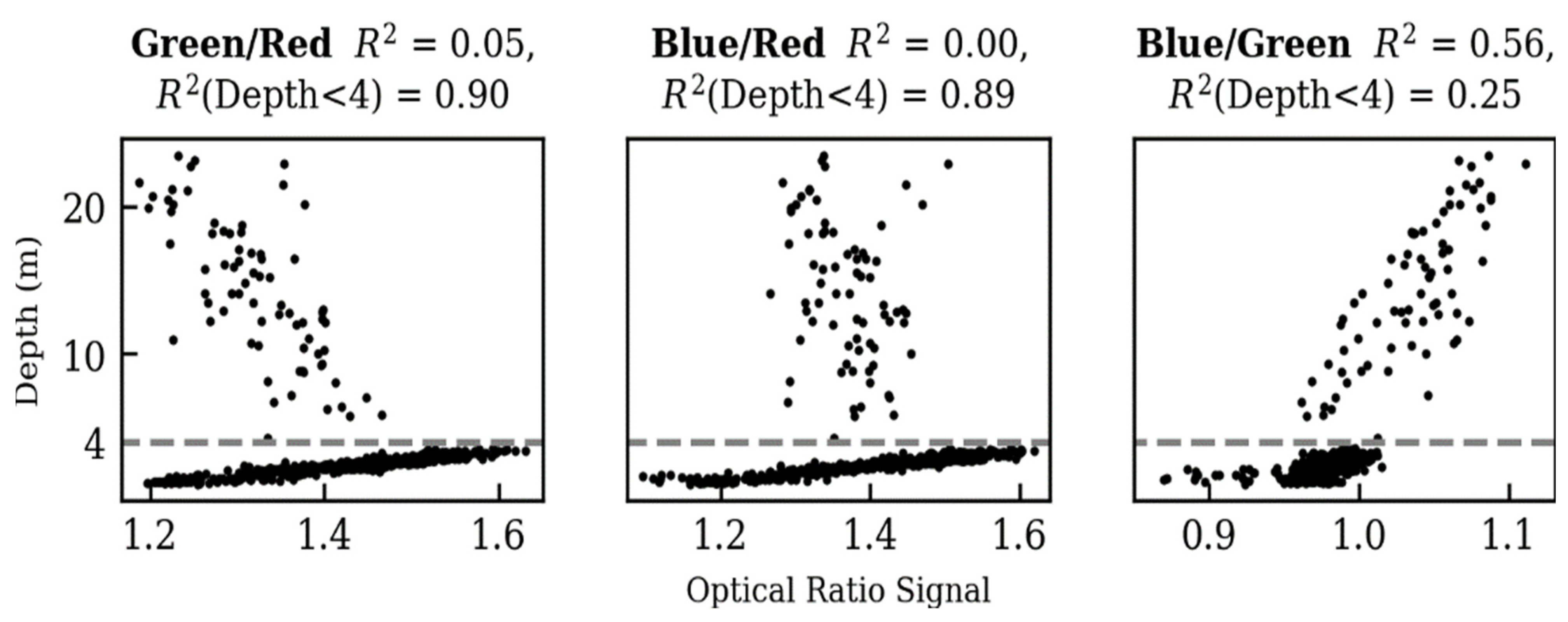
3.1. Single-Band Ratios

As expected, scatterplots of raw band ratios versus measured bathymetry soundings (Figure 3) show variable behaviors depending on the depth level and the selected wavelengths. Band ratios that used the red signal display a drastic change in behavior around a critical depth of about 4 m and display a quite linear relationship for soundings below this threshold. The blue to green ratio (i.e., ratio commonly used by practitioners of the Stumpf algorithm) displays a less straight relation but seems to cover a wider range of depth considering the fairly linear cloud of points between 1 and 20 m.
For single-band ratio models applied to the ELA, the best performances are obtained by the blue to green ratio, but it could only describe approx. 52% of the depth variation (see Supplementary Material Figure S2). Others SBR models performed very poorly in comparison. Once applied to the SLA, single-band ratio models showed opposite results. The amount of depth variation described by the blue to green model is reduced by more 30%, whereas models based on the red band showed a drastic increase in performance, reaching a coefficient of determination of 90% for the green/red SBR model (top and middle panels Figure 4 and Figure 5). However, no acceptable compromise remains as none of the ratios provided suitable solutions for both ELA and SLA areas.

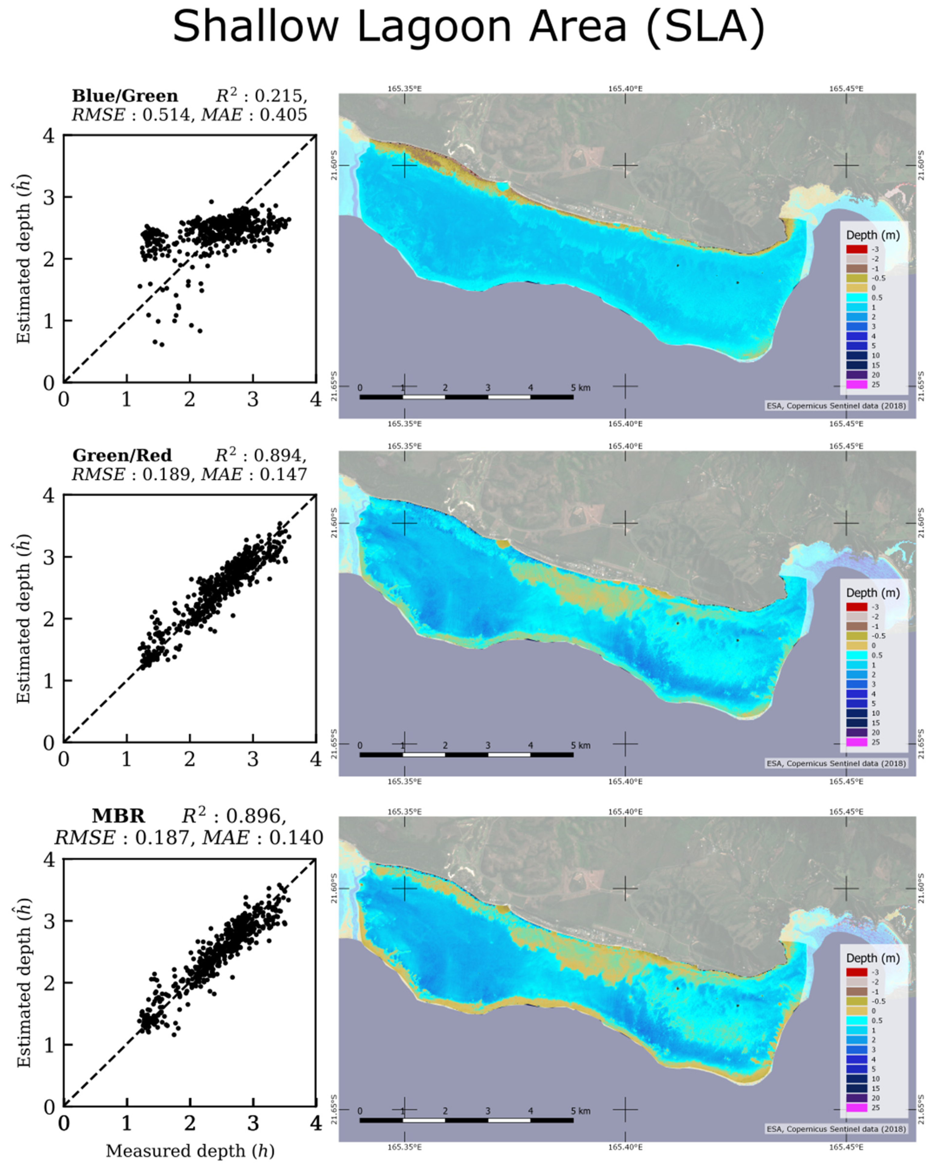
3.2. SBR versus MBR Models Applied on SLA

Stumpf’s model based on the blue to green ratio provided poor results (21.5% of variance explained only and Mean Absolute Error of 0.405 m) when applied to the SLA (Figure 4). It struggles to explain the small gradient of observed depths in this area (between approx. 1 m and 3.5 m) as most of the estimated depths lie between 2 and 3 m. Conversely, the green to red product offers remarkable results in this shallow bathymetric range. It explained almost 90% of the variance of depth, reduced both MAE and RMSE and thus achieved well its objectives. For the SLA, comparatively to the green/red SBR model, MBR provided a slight increase in accuracy. While the percentage of variance explained (89.4 versus 89.6%) is equivalent, the MBR provided notable differences spatially and improved spatial accuracy. Areas with a bathymetry close to the hydrographic zero are more important. The eastern part of the lagoon, known to have a rugose bathymetry, appears less smooth than with a green/red SBR (Figure 4).

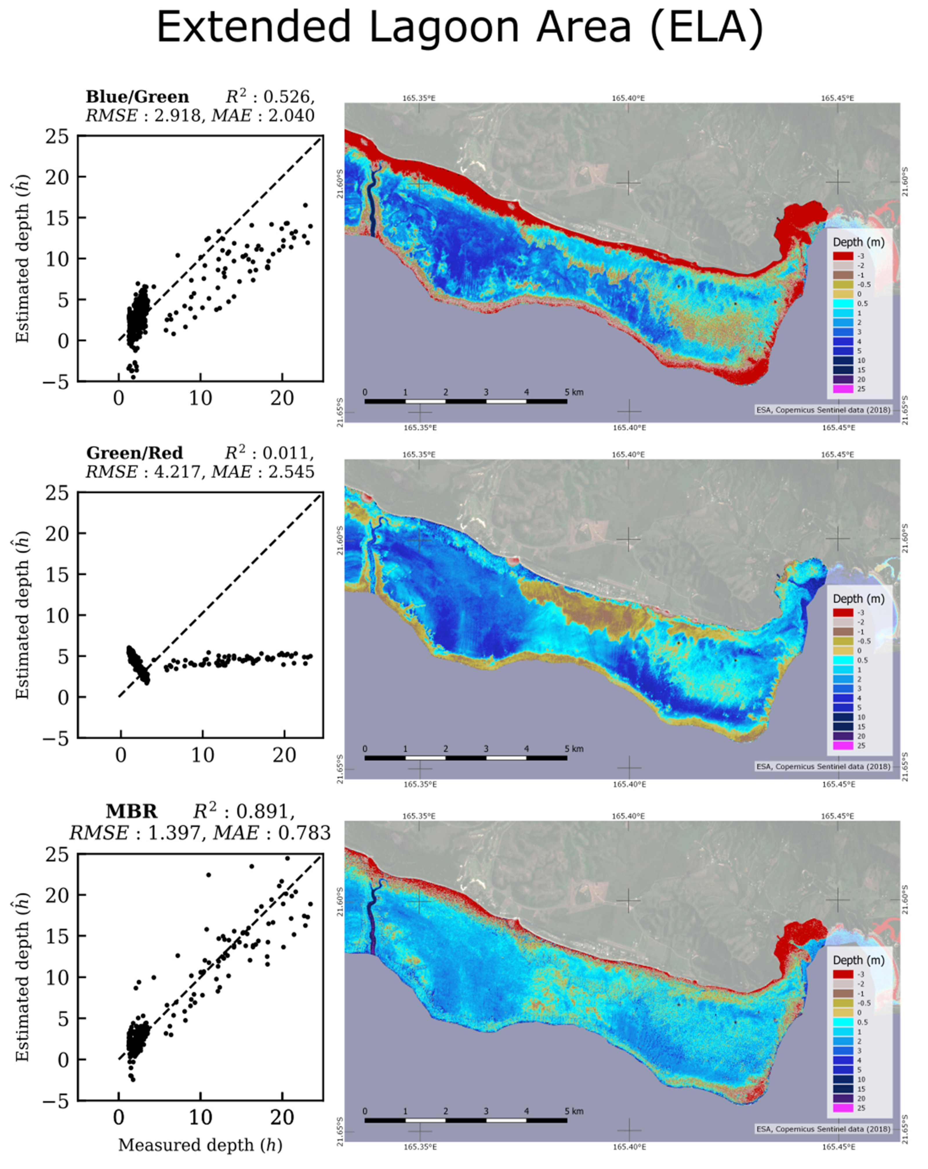
3.3. SBR versus MBR Models Applied on ELA

The green-red SBR and the MBR models calibrated on the SLA allows a precise prediction of depth. Figure 5 displays the results of the same SBR and MBR models but trained this time with the entire soundings dataset, thus including the Sharks Fault. For this extended dataset, the Stumpf model (i.e., the blue to green SBR) provided much better results than the green-red SBR, in line with previous Sentinel-2 studies [22]. The green-red SBR seems particularly inadequate for this range of depths (0–25 m). While the Stumpf blue-green ratio explained up to 52.6% of the variance, it still underestimated soundings over 4 m. The MBR model clearly outperformed the two SBR estimations and explained nearly 90% of the variance. Nevertheless, both the Stumpf and MBR models provided large areas of inaccurate (red in Figure 5) pixels located in the very shallow waters, scattered along the coastline and the barrier reef. With the MBR model, even if known features of the lagoon (e.g., sharp irregularities on its eastern side) seems to be poorly represented, the deep passage is now within a coherent range, from 7 m down to 25 m.

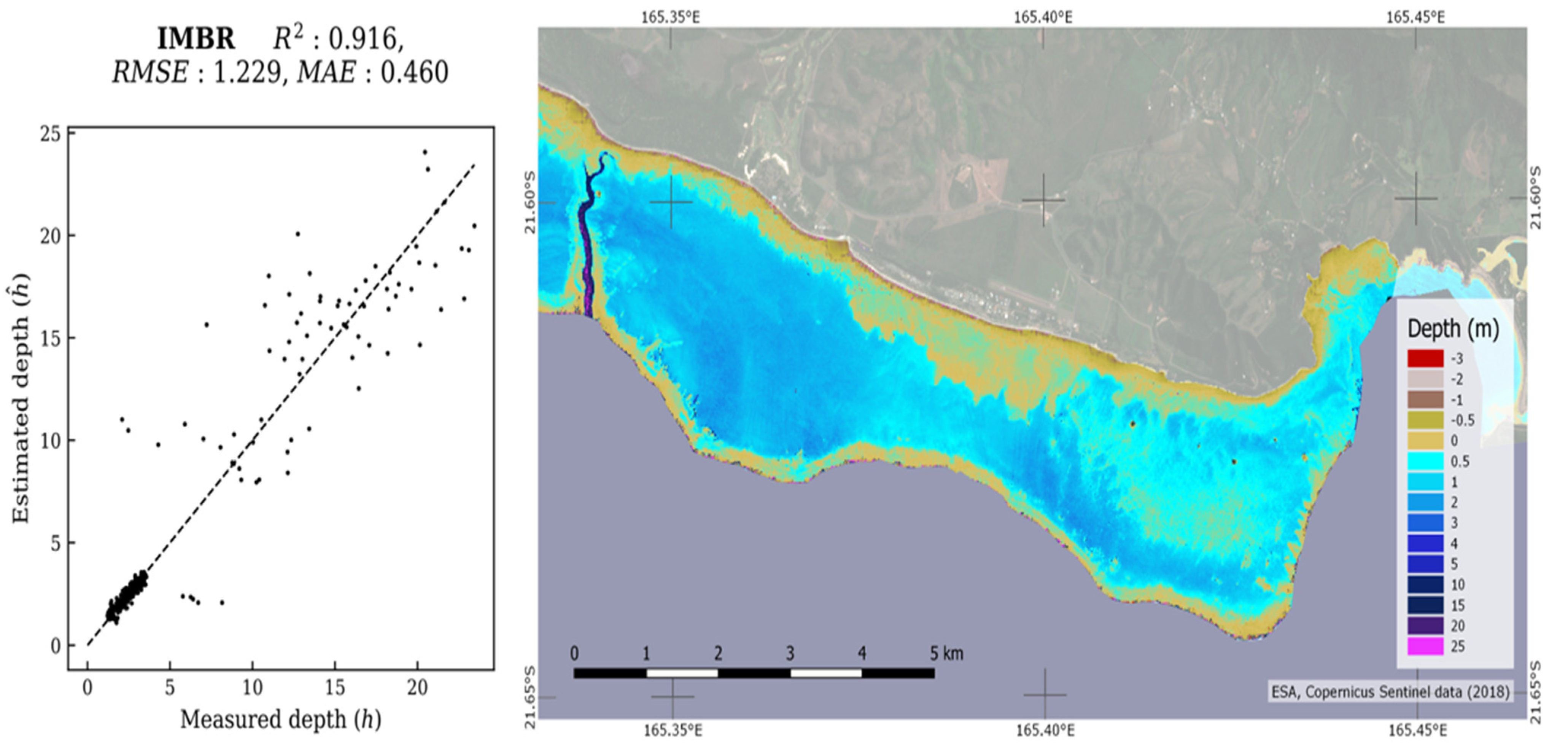
3.4. Results from IMBR on ELA

IMBR, by design, takes full advantage of the various band ratio behaviors presented in Figure 3. Based on Figure 3, an initial threshold has been defined at 4 m; then, empirical optimization led to the definition of two additional thresholds at 5.5 and 12 m as explained above (see Methods Section 2.5.3). Within these two thresholds, three different MBR were implemented with the most suitable bands (Figure 6). Figure 6 shows the evolution of weights (called md in Equation (4)) for every selected SBR depending on the intervals of depths. The importance given to band ratio is also changing along the calibration depth. Among a certain depth interval, negative weight for a specific ratio indicates that the importance of this ratio is quasi-negligible for estimation of depth. For example, green/red ratio is an important component for the 0–5.5 m and 5.5–12 m interval but its influence on bathymetric estimation is insignificant in the last interval (>12 m).
The calibration in two separated steps offers a general improvement of the performance, as seen in Figure 7, with a coefficient of determination reaching 92% and a mean absolute error almost falling by 45%. The greatest enhancement is achieved on the shallow prediction. The mean absolute error in prediction smaller than 4 m is about 16.7 cm, reaching the accuracy level obtained by models calibrated on the shallowest area. Simultaneously, the model is not limited to shallow depths and can predict deeper bathymetry without any strong bias. As a drawback, some outlier predictions remain. For example, two outliers, which are located on the steep ridge of the deep inlet, are strongly over-estimated. Their removals allow us to reach the best accuracy obtained in this study, with a mean absolute error of 13.7 cm for shallow depths (<4 m).
The generalization of the IMBR model is stable, as can be observed in Figure 7. The shallow bathymetry recovers the same level of detail as for MBR predictions over SLA (Figure 4), even in the eastern part of the lagoon. The number of pixels predicted above sea-level remains small and is generally contained in the intertidal zone, where the semi-dry area could be left after the soil thresholding/masking process. The Sharks Fault shows coherent predictions within a range of 7 up to 26 m.

4. Discussion

4.1. Interest of the New IMBR Approach

None of the single-band ratio models are able to properly estimate bathymetry across a wide range of depth. A tradeoff between performances in shallow and deeper areas is needed when selecting bands. Ratios based on longer red wavelengths provide accurate measurements of the shallow area but are unable to provide a valid estimation of deeper bathymetry. In such cases, the denominator band becomes fully attenuated, resulting in an insignificant signal. Conversely, predictions based on shorter wavelength ratios do not saturate within the interval from 0 to 25 m, but they have very low sensitivity in the shallower area, while the deeper areas undergo a light but systematic underestimation. Moreover, the presence of phytoplankton or green vegetation (as in Brisset et al. [61] during a green tide) at a shallow depth likely triggers an increase in the green reflectance. Using this band as the denominator brings the risk of a non-depth-related decrease in the ratio, which can bias shallow estimations.
The multiple-band ratios model overcomes this tradeoff of performances and is now frequently used, e.g., [25,26,40], providing fair estimations simultaneously on both shallow and deep bathymetry. The combination of ratios allows us to better leverage the complementarity of wavelengths which can carry information on different depth levels. However, the multiple-band ratios model is still biased. A significant part of the lagoon is predicted above the sea level, while the rugosity of the eastern part of the lagoon remains poorly represented. Indeed, as shown in Figure 3, the complete attenuation of the denominator bands results in a drastic change in the behavior of some ratios, around a critical depth. These inconsistent behaviors, together with the use of a unique linear solution, prevent the model from fully leveraging shorter-wavelength bands at a shallow depth.
The iterative multiple-bands ratio model is fully leveraging complementarity of wavelengths. It provides the most accurate estimation on shallow areas according to our tests on both SLA and ELA. As a first step, it takes advantage of the ability of the MBR model to provide fair estimation, regardless of the depth level. In a second step, it refines the estimation thanks to an optimal model dedicated to a narrower depth range. Nevertheless, few outliers and erroneous above-sea-level predictions may remain. These are mainly due to mis-classification during the first step. In addition, we acknowledge that the definition of depth threshold is not yet automatized, but further systematical incremental analysis showed that these two thresholds were the pair of values yielding the most reliable estimations (See Supplementary Material Figure S1). Readers are invited to apply the same analysis should they apply the method presented here.

4.2. The Use of Sentinel-2 Imagery

This paper demonstrates that the choice of Sentinel-2 imagery was quite satisfactory. Firstly, the native spatial resolution of Sentinel-2 scenes (10 m for 3 bands) is fully appropriate for building a high-resolution hydrodynamic model of New Caledonia lagoons, and to represent realistically sharp depth variations. The good results achieved here bring confidence for the further developments of these models. It must be however pointed out the need to resample the 20 m (extra-red band) and 60 m (extra-blue band) bands to take advantage of the portfolio of all possible band ratios. In some very rugose areas, this can be a limitation if ratios based on these two bands are effective. However, here, the best results were achieved with the contribution of the 10 m bands (see Figure 5, Figure 6 and Figure 7).
Second, with its straightforward, open-access delivery time and frequency of revisit (5 days), the whole mission offered a wide choice of available images, which is critical to avoid images polluted by cloud, waves, turbid plumes, etc. Selecting an image with a clear atmosphere and water column is critical for maximizing the performances of any algorithm. The flexibility brought by the Sentinel-2 image portal and tested for the Poe Lagoon is generalizable to the different New Caledonian lagoons. Many lagoons (but not all, as was the case for Poe before this study) have a good coverage of publicly available depth sounding data (by the French hydrographic survey offices) in a variety of depth ranges. That should allow the fast processing of other New Caledonia lagoons within the 0–30 m depth range at most. A first demonstration of generalization is provided with Figure 8 example, with a series of new Caledonian west coast lagoons in the same depth ranges and bottom types as Poe lagoon. In this case, we used the entire footprint of the Poe lagoon image and applied the IMBR calibrated on Poe soundings to this wider zone. Estimation of depth is coherent with patterns visible on the true-color images and based on our knowledge of these sites. Obviously, an independent ground-truth survey will quantify the errors, and also optimize the process locally should the Poe parameterization prove to be sub-optimal for these other lagoons.
Using the continuous growth of the Sentinel-2 archive also allows us to revisit areas that had to be processed with sub-optimal images (due to clouds, for instance, etc.), and/or revisit areas that could be affected by large disturbances that have the potentials to modify coastlines and shallow lagoons such as cyclones, floods or large swells [62].

4.3. Portfolio of Methods for Practitionners

The number of published methods to estimate bathymetry is wide and continues to expand, with several new references each year. In front of the wide portfolio of methods, it seems reasonable to recommend to practitioners and users of bathymetry products that are not remote sensing specialists to have a good understanding of their needs first. Indeed, the requirements are very variable from numerical modelers in search of very accurate products (in our case) to ecologists requesting a coarse level to characterize species habitats and who could be happy with a single-band ratio method and a low precision of few-meter accuracy. It also does not face the same challenges and choices when the sizes of targeted areas range from the entire New Caledonia (~20.000 km2 of reefs and lagoons) to a single lagoon or bay covering a few km2 at most. The review Section 2.1 summarizes the main types of algorithms available to date. Most have variations and different potential based on different images, which can range from MERIS at 300 m spatial resolution data to numerous multispectral-derived products at 1 to 10 m resolution, including Sentinel images, and to hyperspectral airborne images. Other important constraints include the access to a minimum set of ground-truth data, necessary for calibration and reaching good accuracy. Dense and regular surveys are difficult and costly to acquire and can be a challenge in some very shallow lagoon inaccessible even to small vessels.
Specifically, for New Caledonia, the next steps are to systematically map the bathymetry of the lagoons for which numerical models are being developed, and still using Sentinel-2 images. Elsewhere, in all coral reef provinces worldwide, it is possible to identify shallow lagoons intersected by deep passes where the approach described here can be usefully applied.

5. Conclusions

Using a New Caledonian lagoon example, the results of the study confirmed the limitations of Single-Band Ratio (SBR) algorithms that performed well on shallow and deep areas separately, as long as the suitable bands were used. Applying this method for rugose previously uncharted lagoons is, however, impractical as it requires a careful delimitation of each shallow and deep area to fit and apply separate models. Applying SBR models across the entire lagoon yielded average results.
The simultaneous use of Multiple-Band Ratios (MBR) has partially overcome the SBR algorithm limitations. When calibrated on the whole lagoon, SBR models were clearly outperformed by the MBR model on both shallow and deep areas. Yet, the MBR model did not achieve the best performances, obtained with dedicated SBR models, specifically fitted for the targeted depths.
Finally, the Iterative Multiple Band Ratios (IMBR) model addressed all limitations and reduced the average absolute error by more than 40% in some configurations. In shallow areas, IMBR outperformed MBR with an average absolute error of the same order as dedicated SBR models, while being calibrated on the whole lagoon. The IMBR model could address the entire depth range of the study area with a single procedure, which was accurate for both shallow details and deep channels.
Combined with the IMBR method, Sentinel-2 data proved to be a useful source of information for bathymetry retrieval, offering for our needs a satisfying ground resolution. This potential is strengthened by the mission revisit time which increases the probability to access free images of high environmental quality.

Supplementary Materials

The following are available online at https://0-www-mdpi-com.brum.beds.ac.uk/article/10.3390/rs13204108/s1, Figure S1: Influence of the choice of threshold pair on the IMBR performance (RMSE, MAE, R2). White rectangles showing best areas of thresholds combination. Figure S2: All possible combinations of SBR model outputs compared with in situ data on ELA. Accuracy metrics are provided above each validation plot.

Author Contributions

Conceptualization, S.A. (Sélim Amrari), R.L.G., B.S. and H.L.; methodology, S.A. (Sélim Amrari), R.L.G., B.S.; software, S.A. (Sélim Amrari), E.B.; validation, S.A. (Sélim Amrari), E.B., R.L.G.; formal analysis, S.A. (Sélim Amrari); investigation, S.A. (Sélim Amrari), R.L.G., B.S. and H.L.; resources, S.A. (Sélim Amrari); data curation, S.A. (Sélim Amrari) and E.B.; writing—original draft preparation, S.A. (Sélim Amrari), R.L.G., S.A. (Serge Andréfouët); writing—review and editing, B.S., E.B., R.L.G., S.A. (Sélim Amrari) and S.A. (Serge Andréfouët); visualization, S.A. (Sélim Amrari), E.B. and R.L.G.; supervision, R.L.G., B.S. and H.L.; project administration, B.S.; funding acquisition, R.L.G., B.S. and H.L. All authors have read and agreed to the published version of the manuscript.

Funding

This work was funded by New Caledonia institutions (Government, South Province, North Province) within the PRESENCE (PRESsures on coral Ecosystems of New CalEdonia) scientific project.

Data Availability Statement

The data presented in this study are openly available at [https://sextant.ifremer.fr, accessed on 15 September 2021].

Acknowledgments

The authors are grateful to José Herlin and Eric Le Tesson for their participation in data collection.

Conflicts of Interest

The authors declare no conflict of interest.

References

  1. Brock, J.; Yates, K.; Halley, R.; Kuffner, I.; Wright, C.; Hatcher, B. Northern Florida Reef Tract Benthic Metabolism Scaled by Remote Sensing. Mar. Ecol. Prog. Ser. 2006, 312, 123–139. [Google Scholar] [CrossRef] [Green Version]
  2. Harris, P.M.; Purkis, S.J.; Ellis, J.; Swart, P.K.; Reijmer, J.J.G. Mapping Bathymetry and Depositional Facies on Great Bahama Bank. Sedimentology 2015, 62, 566–589. [Google Scholar] [CrossRef]
  3. Purkis, S.J.; Rowlands, G.P.; Kerr, J.M. Unravelling the Influence of Water Depth and Wave Energy on the Facies Diversity of Shelf Carbonates. Sedimentology 2015, 62, 541–565. [Google Scholar] [CrossRef]
  4. Bridge, T.C.L.; Hoey, A.S.; Campbell, S.J.; Muttaqin, E.; Rudi, E.; Fadli, N.; Baird, A.H. Depth-dependent mortality of reef corals following a severe bleaching event: implications for thermal refuges and population recovery. F1000Research 2013, 2, 187. [Google Scholar] [CrossRef] [PubMed]
  5. Reguero, B.G.; Beck, M.W.; Agostini, V.N.; Kramer, P.; Hancock, B. Coral Reefs for Coastal Protection: A New Methodological Approach and Engineering Case Study in Grenada. J. Environ. Manag. 2018, 210, 146–161. [Google Scholar] [CrossRef] [PubMed]
  6. Andréfouët, S.; Ouillon, S.; Brinkman, R.; Falter, J.; Douillet, P.; Wolk, F.; Smith, R.; Garen, P.; Martinez, E.; Laurent, V.; et al. Review of Solutions for 3D Hydrodynamic Modeling Applied to Aquaculture in South Pacific Atoll Lagoons. Mar. Pollut. Bull. 2006, 52, 1138–1155. [Google Scholar] [CrossRef] [PubMed]
  7. Ye, F.; Zhang, Y.J.; Wang, H.V.; Friedrichs, M.A.M.; Irby, I.D.; Alteljevich, E.; Valle-Levinson, A.; Wang, Z.; Huang, H.; Shen, J.; et al. A 3D Unstructured-Grid Model for Chesapeake Bay: Importance of Bathymetry. Ocean Model. 2018, 127, 16–39. [Google Scholar] [CrossRef] [Green Version]
  8. Pydyn, A.; Popek, M.; Kubacka, M.; Janowski, Ł. Exploration and reconstruction of a medieval harbour using hydroacoustics, 3-D shallow seismic and underwater photogrammetry: A case study from Puck, southern Baltic Sea. Archaeol. Prospect. 2021, 1–16. [Google Scholar] [CrossRef]
  9. Micallef, A.; Foglini, F.; Le Bas, T.; Angeletti, L.; Maselli, V.; Pasuto, A.; Taviani, M. The submerged paleolandscape of the Maltese Islands: Morphology, evolution and relation to Quaternary environmental change. Mar. Geol. 2013, 335, 129–147. [Google Scholar] [CrossRef]
  10. Payri, C.E.; Allain, V.; Aucan, J.; David, C.; David, V.; Dutheil, C.; Loubersac, L.; Menkes, C.; Pelletier, B.; Pestana, G.; et al. New Caledonia. In World Seas: An Environmental Evaluation; Elsevier: Amsterdam, The Netherlands, 2019; pp. 593–618. ISBN 978-0-08-100853-9. [Google Scholar]
  11. Ouillon, S.; Douillet, P.; Lefebvre, J.P.; Le Gendre, R.; Jouon, A.; Bonneton, P.; Fernandez, J.M.; Chevillon, C.; Magand, O.; Lefèvre, J.; et al. Circulation and Suspended Sediment Transport in a Coral Reef Lagoon: The South-West Lagoon of New Caledonia. Mar. Pollut. Bull. 2010, 61, 269–296. [Google Scholar] [CrossRef] [Green Version]
  12. Andréfouët, S.; Cabioch, G.; Flamand, B.; Pelletier, B. A Reappraisal of the Diversity of Geomorphological and Genetic Processes of New Caledonian Coral Reefs: A Synthesis from Optical Remote Sensing, Coring and Acoustic Multibeam Observations. Coral Reefs 2009, 28, 691–707. [Google Scholar] [CrossRef]
  13. Manessa, M.D.M.; Kanno, A.; Sagawa, T.; Sekine, M.; Nurdin, N. Simulation-Based Investigation of the Generality of Lyzenga’s Multispectral Bathymetry Formula in Case-1 Coral Reef Water. Estuar. Coast. Shelf Sci. 2018, 200, 81–90. [Google Scholar] [CrossRef]
  14. Garcia, R.A.; Fearns, P.R.C.S.; McKinna, L.I.W. Detecting Trend and Seasonal Changes in Bathymetry Derived from HICO Imagery: A Case Study of Shark Bay, Western Australia. Remote Sens. Environ. 2014, 147, 186–205. [Google Scholar] [CrossRef] [Green Version]
  15. Pacheco, A.; Horta, J.; Loureiro, C.; Ferreira, Ó. Retrieval of Nearshore Bathymetry from Landsat 8 Images: A Tool for Coastal Monitoring in Shallow Waters. Remote Sens. Environ. 2015, 159, 102–116. [Google Scholar] [CrossRef] [Green Version]
  16. Mobley, C.D. Light and Water: Radiative Transfer in Natural Waters; Academic Press: Cambridge, MA, USA, 1994. [Google Scholar]
  17. Maritorena, S.; Morel, A.; Gentili, B. Diffuse Reflectance of Oceanic Shallow Waters: Influence of Water Depth and Bottom Albedo. Limnol. Oceanogr. 1994, 39, 1689–1703. [Google Scholar] [CrossRef]
  18. Kutser, T.; Hedley, J.; Giardino, C.; Roelfsema, C.; Brando, V.E. Remote Sensing of Shallow Waters–A 50 Year Retrospective and Future Directions. Remote Sens. Environ. 2020, 240, 111619. [Google Scholar] [CrossRef]
  19. Morel, Y.; Favoretto, F. 4SM: A Novel Self-Calibrated Algebraic Ratio Method for Satellite-Derived Bathymetry and Water Column Correction. Sensors 2017, 17, 1682. [Google Scholar] [CrossRef] [PubMed]
  20. Liang, J.; Zhang, J.; Ma, Y.; Zhang, C.-Y. Derivation of Bathymetry from High-Resolution Optical Satellite Imagery and USV Sounding Data. Mar. Geod. 2017, 40, 466–479. [Google Scholar] [CrossRef]
  21. Hedley, J.D.; Roelfsema, C.; Brando, V.; Giardino, C.; Kutser, T.; Phinn, S.; Mumby, P.J.; Barrilero, O.; Laporte, J.; Koetz, B. Coral Reef Applications of Sentinel-2: Coverage, Characteristics, Bathymetry and Benthic Mapping with Comparison to Landsat 8. Remote Sens. Environ. 2018, 216, 598–614. [Google Scholar] [CrossRef]
  22. Caballero, I.; Stumpf, R.P. Retrieval of nearshore bathymetry from Sentinel-2A and 2B satellites in South Florida coastal waters. Estuar. Coast. Shelf Sci. 2019, 226, 106277. [Google Scholar] [CrossRef]
  23. Casal, G.; Harris, P.; Monteys, X.; Hedley, J.; Cahalane, C.; McCarthy, T. Understanding satellite-derived bathymetry using Sentinel 2 imagery and spatial prediction models. GIScience Remote Sens. 2020, 57, 271–286. [Google Scholar] [CrossRef]
  24. Traganos, D.; Poursanidis, D.; Aggarwal, B.; Chrysoulakis, N.; Reinartz, P. Estimating Satellite-Derived Bathymetry (SDB) with the Google Earth Engine and Sentinel-2. Remote Sens. 2018, 10, 859. [Google Scholar] [CrossRef] [Green Version]
  25. Kerr, J.M.; Purkis, S. An Algorithm for Optically-Deriving Water Depth from Multispectral Imagery in Coral Reef Landscapes in the Absence of Ground-Truth Data. Remote Sens. Environ. 2018, 210, 307–324. [Google Scholar] [CrossRef]
  26. Purkis, S.J.; Gleason, A.C.R.; Purkis, C.R.; Dempsey, A.C.; Renaud, P.G.; Faisal, M.; Saul, S.; Kerr, J.M. High-Resolution Habitat and Bathymetry Maps for 65,000 Sq. Km of Earth’s Remotest Coral Reefs. Coral Reefs 2019, 38, 467–488. [Google Scholar] [CrossRef] [Green Version]
  27. Li, J.; Knapp, D.E.; Schill, S.R.; Roelfsema, C.; Phinn, S.; Silman, M.; Mascaro, J.; Asner, G.P. Adaptive Bathymetry Estimation for Shallow Coastal Waters Using Planet Dove Satellites. Remote Sens. Environ. 2019, 232, 111302. [Google Scholar] [CrossRef]
  28. Caballero, I.; Stumpf, R.P. Atmospheric Correction for Satellite-Derived Bathymetry in the Caribbean Waters: From a Single Image to Multi-Temporal Approaches Using Sentinel-2A/B. Opt. Express 2020, 28, 11742. [Google Scholar] [CrossRef] [PubMed]
  29. Minghelli-Roman, A.; Dupouy, C. Correction of the Water Column Attenuation: Application to the Seabed Mapping of the Lagoon of New Caledonia Using MERIS Images. IEEE J. Sel. Top. Appl. Earth Obs. Remote Sens. 2014, 7, 2619–2629. [Google Scholar] [CrossRef] [Green Version]
  30. Hedley, J.; Roelfsema, C.; Koetz, B.; Phinn, S. Capability of the Sentinel 2 Mission for Tropical Coral Reef Mapping and Coral Bleaching Detection. Remote Sens. Environ. 2012, 120, 145–155. [Google Scholar] [CrossRef]
  31. Dörnhöfer, K.; Göritz, A.; Gege, P.; Pflug, B.; Oppelt, N. Water Constituents and Water Depth Retrieval from Sentinel-2A—A First Evaluation in an Oligotrophic Lake. Remote. Sens. 2016, 8, 941. [Google Scholar] [CrossRef] [Green Version]
  32. Chybicki, A. Mapping South Baltic Near-Shore Bathymetry Using Sentinel-2 Observations. Pol. Marit. Res. 2017, 24, 15–25. [Google Scholar] [CrossRef]
  33. Chybicki, A. Three-Dimensional Geographically Weighted Inverse Regression (3GWR) Model for Satellite Derived Bathymetry Using Sentinel-2 Observations. Mar. Geod. 2018, 41, 1–23. [Google Scholar] [CrossRef]
  34. Poursanidis, D.; Traganos, D.; Reinartz, P.; Chrysoulakis, N. On the use of Sentinel-2 for coastal habitat mapping and satellite-derived bathymetry estimation using downscaled coastal aerosol band. Int. J. Appl. Earth Obs. Geoinf. 2019, 80, 58–70. [Google Scholar] [CrossRef]
  35. Lyzenga, D.R. Passive Remote Sensing Techniques for Mapping Water Depth and Bottom Features. Appl. Opt. 1978, 17, 379. [Google Scholar] [CrossRef] [PubMed]
  36. Lyzenga, D.R.; Malinas, N.P.; Tanis, F.J. Multispectral Bathymetry Using a Simple Physically Based Algorithm. IEEE Trans. Geosci. Remote Sens. 2006, 44, 2251–2259. [Google Scholar] [CrossRef]
  37. Philpot, W.D. Bathymetric Mapping with Passive Multispectral Imagery. Appl. Opt. 1989, 28, 1569. [Google Scholar] [CrossRef] [PubMed]
  38. Stumpf, R.P.; Holderied, K.; Sinclair, M. Determination of Water Depth with High-Resolution Satellite Imagery over Variable Bottom Types. Limnol. Oceanogr. 2003, 48, 547–556. [Google Scholar] [CrossRef]
  39. Lyons, M.; Phinn, S.; Roelfsema, C. Integrating Quickbird Multi-Spectral Satellite and Field Data: Mapping Bathymetry, Seagrass Cover, Seagrass Species and Change in Moreton Bay, Australia in 2004 and 2007. Remote Sens. 2011, 3, 42–64. [Google Scholar] [CrossRef] [Green Version]
  40. Niroumand-Jadidi, M.; Bovolo, F.; Bruzzone, L. SMART-SDB: Sample-Specific Multiple Band Ratio Technique for Satellite-Derived Bathymetry. Remote Sens. Environ. 2020, 251, 112091. [Google Scholar] [CrossRef]
  41. Su, H.; Liu, H.; Wang, L.; Filippi, A.M.; Heyman, W.D.; Beck, R.A. Geographically Adaptive Inversion Model for Improving Bathymetric Retrieval from Satellite Multispectral Imagery. IEEE Trans. Geosci. Remote Sens. 2014, 52, 465–476. [Google Scholar] [CrossRef]
  42. Vinayaraj, P.; Raghavan, V.; Masumoto, S. Satellite-Derived Bathymetry Using Adaptive Geographically Weighted Regression Model. Mar. Geod. 2016, 39, 458–478. [Google Scholar] [CrossRef]
  43. Manessa, M.D.M.; Kanno, A.; Sekine, M.; Haidar, M.; Yamamoto, K.; Imai, T.; Higuchi, T. Satellite-Derived Bathymetry Using Random Forest Algorithm and Worldview-2 Imagery. Geoplanning J. Geomat. Plan. 2016, 3, 117. [Google Scholar] [CrossRef] [Green Version]
  44. Ceyhun, Ö.; Yalçın, A. Remote Sensing of Water Depths in Shallow Waters via Artificial Neural Networks. Estuar. Coast. Shelf Sci. 2010, 89, 89–96. [Google Scholar] [CrossRef]
  45. Makboul, O.; Negm, A.; Mesbah, S.; Mohasseb, M. Performance Assessment of ANN in Estimating Remotely Sensed Extracted Bathymetry. Case Study: Eastern Harbor of Alexandria. Procedia Eng. 2017, 181, 912–919. [Google Scholar] [CrossRef]
  46. Hochberg, E.J.; Andrefouet, S.; Tyler, M.R. Sea Surface Correction of High Spatial Resolution Ikonos Images to Improve Bottom Mapping in Near-Shore Environments. IEEE Trans. Geosci. Remote Sens. 2003, 41, 1724–1729. [Google Scholar] [CrossRef]
  47. Vanhellemont, Q.; Ruddick, K. Acolite For Sentinel-2: Aquatic Applications of Msi Imagery. In Proceedings of the 2016 ESA Living Planet Symposium, Prague, Czech Republic, 9–13 May 2016; Volume 8, pp. 9–13. [Google Scholar]
  48. Vermote, E.; Tanré, D.; Deuzé, J.L.; Herman, M.; Morcrette, J.J.; Kotchenova, S.Y. Second simulation of a satellite signal in the solar spectrum-vector (6SV). 6S User Guid. 2006, 1–55. Available online: https://salsa.umd.edu/files/6S/6S_Manual_Part_1.pdf (accessed on 15 September 2021).
  49. Vanhellemont, Q.; Ruddick, K. Atmospheric Correction of Metre-Scale Optical Satellite Data for Inland and Coastal Water Applications. Remote Sens. Environ. 2018, 216, 586–597. [Google Scholar] [CrossRef]
  50. Vanhellemont, Q. Adaptation of the Dark Spectrum Fitting Atmospheric Correction for Aquatic Applications of the Landsat and Sentinel-2 Archives. Remote Sens. Environ. 2019, 225, 175–192. [Google Scholar] [CrossRef]
  51. Jupp, D.L.B. Background and extensions to depth of penetration (DOP) mapping in shallow coastal waters. In Proceedings of the Remote Sensing of the Coastal Zone International Symposium, Gold Coast, Australia, 1988; pp. IV.2.1–IV.2.19. [Google Scholar]
  52. Lee, Z.-P. Diffuse Attenuation Coefficient of Downwelling Irradiance: An Evaluation of Remote Sensing Methods. J. Geophys. Res. 2005, 110, C02017. [Google Scholar] [CrossRef]
  53. Mishra, D.R.; Narumalani, S.; Rundquist, D.; Lawson, M. Characterizing the Vertical Diffuse Attenuation Coefficient for Downwelling Irradiance in Coastal Waters: Implications for Water Penetration by High Resolution Satellite Data. ISPRS J. Photogramm. Remote Sens. 2005, 60, 48–64. [Google Scholar] [CrossRef]
  54. Doxani, G.; Papadopoulou, M.; Lafazani, P.; Pikridas, C.; Tsakiri-Strati, M. Shallow-water bathymetry over variable bottom types using multispectral worldview-2 image. Int. Arch. Photogramm. Remote Sens. Spat. Inf. Sci. 2012, XXXIX-B8, 159–164. [Google Scholar] [CrossRef] [Green Version]
  55. Niroumand-Jadidi, M.; Vitti, A. Optimal band ratio analysis of worldview-3 imagery for bathymetry of shallow rivers (case study: sarca river, italy). Int. Arch. Photogramm. Remote Sens. Spat. Inf. Sci. 2016, XLI-B8, 361–364. [Google Scholar] [CrossRef] [Green Version]
  56. Figueiredo, I.N.; Pinto, L.; Goncalves, G. A Modified Lyzenga’s Model for Multispectral Bathymetry Using Tikhonov Regularization. IEEE Geosci. Remote Sens. Lett. 2016, 13, 53–57. [Google Scholar] [CrossRef]
  57. Tikhonov, A.N. Solution of incorrectly formulated problems and the regularization method. Sov. Math. Dokl. 1963, 4, 1035–1038. [Google Scholar]
  58. Hoerl, A.E.; Kennard, R.W. Ridge Regression: Biased Estimation for Nonorthogonal Problems. Technometrics 1970, 12, 55–67. [Google Scholar] [CrossRef]
  59. Roberts, D.R.; Bahn, V.; Ciuti, S.; Boyce, M.S.; Elith, J.; Guillera-Arroita, G.; Hauenstein, S.; Lahoz-Monfort, J.J.; Schröder, B.; Thuiller, W.; et al. Cross-Validation Strategies for Data with Temporal, Spatial, Hierarchical, or Phylogenetic Structure. Ecography 2017, 40, 913–929. [Google Scholar] [CrossRef]
  60. Trachsel, M.; Telford, R.J. Technical Note: Estimating Unbiased Transfer-Function Performances in Spatially Structured Environments. Clim. Past 2016, 12, 1215–1223. [Google Scholar] [CrossRef] [Green Version]
  61. Brisset, M.; Van Wynsberge, S.; Andréfouët, S.; Payri, C.; Soulard, B.; Bourassin, E.; Le Gendre, R.; Coutures, E. Hindcast and Near Real-Time Monitoring of Green Macroalgae Blooms in Shallow Coral Reef Lagoons Using Sentinel-2: A New-Caledonia Case Study. Remote Sens. 2021, 13, 211. [Google Scholar] [CrossRef]
  62. Jullien, S.; Aucan, J.; Lefèvre, J.; Peltier, A.; Menkes, C.E. Tropical cyclone induced wave setup around New Caledonia during Cyclone COOK (2017). J. Coast. Res. 2020, 95, 1454–1459. [Google Scholar] [CrossRef]
Figure 1. Location of the study site (red dot on the lower-left thumbnail). Sentinel-2 image of the Poe lagoon (5 March 2018), including toponyms, tracks of in situ depth soundings (yellow dots), limits of the shallow lagoon area (purple) and the limit of the extended area that includes the Sharks Fault pass (red).
Remotesensing 13 04108 g001
Figure 2. Processing workflow; within its center, the three ratio approaches that are compared here for Poe lagoon.
Remotesensing 13 04108 g002
Figure 3. Examples of depth versus computed single-band optical ratios. Coefficients of determination R2 are displayed for the entire ground-truth dataset and for depth < 4 m.
Remotesensing 13 04108 g003
Figure 4. Applications to the SLA of the blue/green SBR model (top), the green-red SBR model (middle) and the MBR model (bottom). Accuracy metrics are provided above each validation plot on the left-inside.
Remotesensing 13 04108 g004
Figure 5. Applications to the ELA of the blue/green SBR model (top), the green-red SBR model (middle) and the MBR model (bottom). Predictions are at zero hydrographic level; therefore, red pixels are incoherent predictions, estimated above sea level. Accuracy metrics are provided above each validation plot on the left-inside.
Remotesensing 13 04108 g005
Figure 6. Evolution of the ratio weights (md Equation (4)) over the three depth intervals of calibration.
Remotesensing 13 04108 g006
Figure 7. IMBR-derived bathymetry for the ELA (calibration on the global dataset). Predictions are at zero hydrographic level; therefore, the very few red pixels on prediction maps are incoherent prediction, estimated above sea level. Accuracy metrics are provided above the validation plot.
Remotesensing 13 04108 g007
Figure 8. Up–Application of the IMBR model over the footprint of the same Sentinel-2 scene processed for the Poe lagoon. (a) zoom on the Poya lagoon; (b) zoom on the Sharks fault and surroundings; (c) zoom on the Moindou lagoon.
Remotesensing 13 04108 g008
Table 1. Sentinel-2 spectral and spatial characteristics.
Band NameCentral Wavelength (nm)Spectral Bandwidth (nm)Spatial Resolution (m)
Extra (shorter) Blue443.92760
Blue496.69810
Green560.04510
Red664.53810
Extra (longer) Red703.01920
Publisher’s Note: MDPI stays neutral with regard to jurisdictional claims in published maps and institutional affiliations.

