
Source Model and Simulated Strong Ground Motion of the 2021 Yangbi, China Shallow Earthquake Constrained by InSAR Observations

 , ,
, ,
Abstract
:1. Introduction
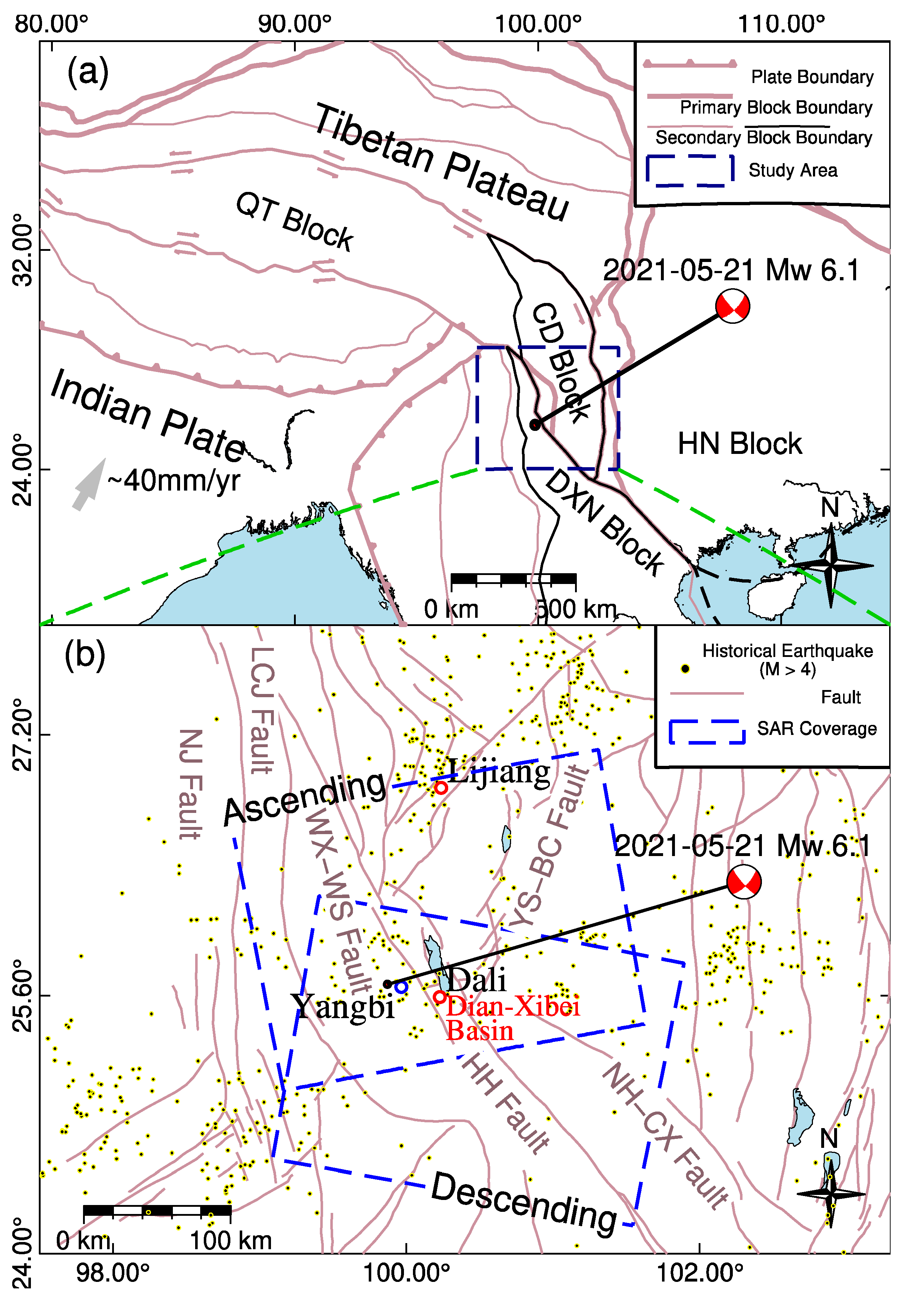
2. Tectonic Setting
3. Data and Methods
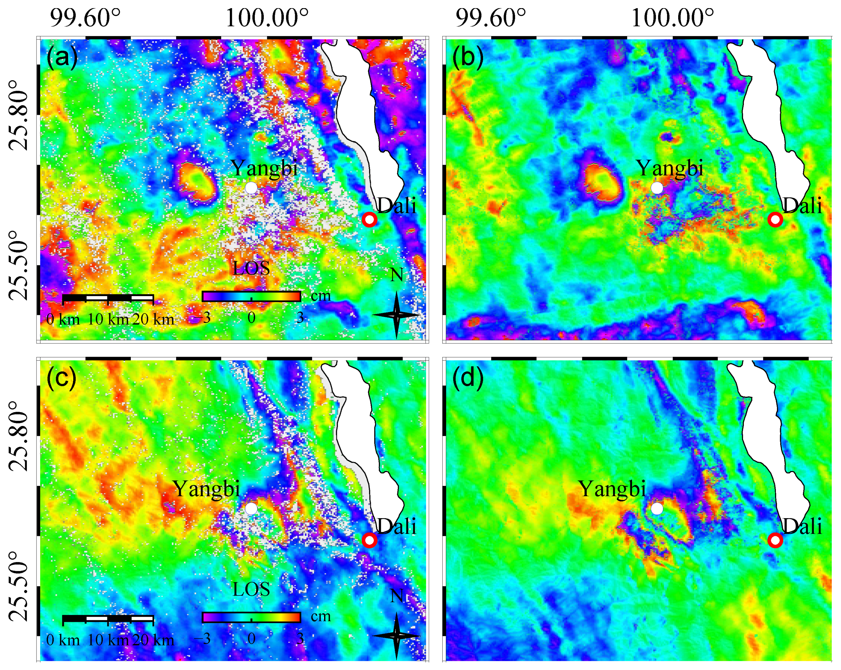
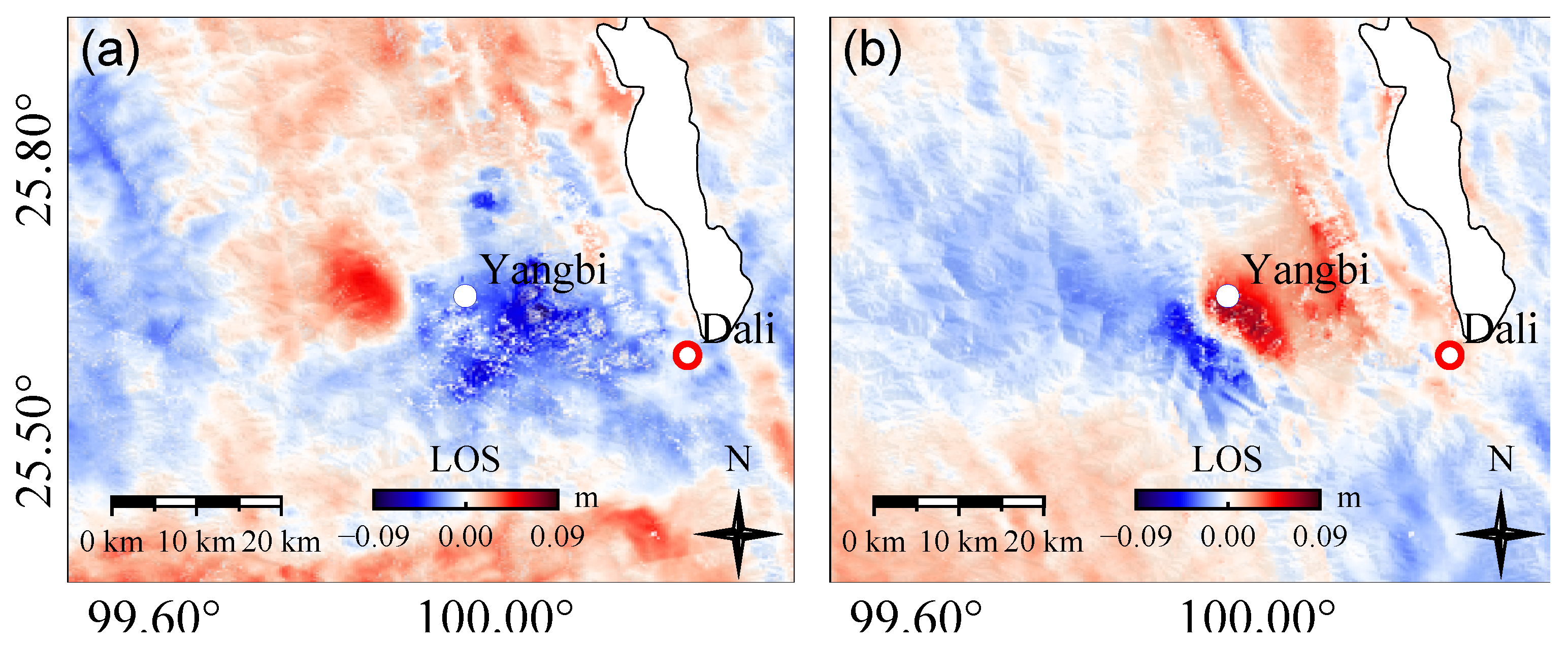
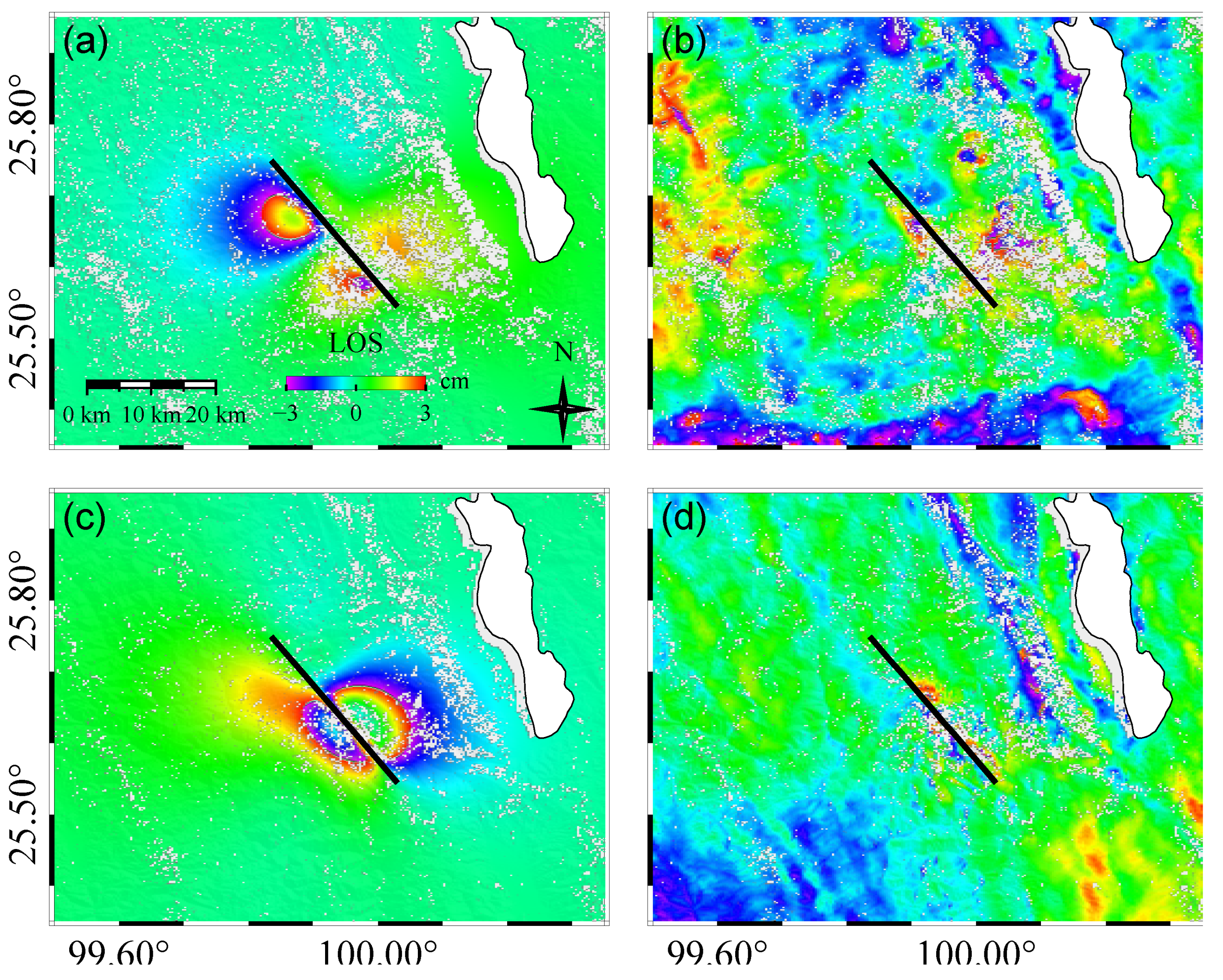
3.1. SAR Data and Processing
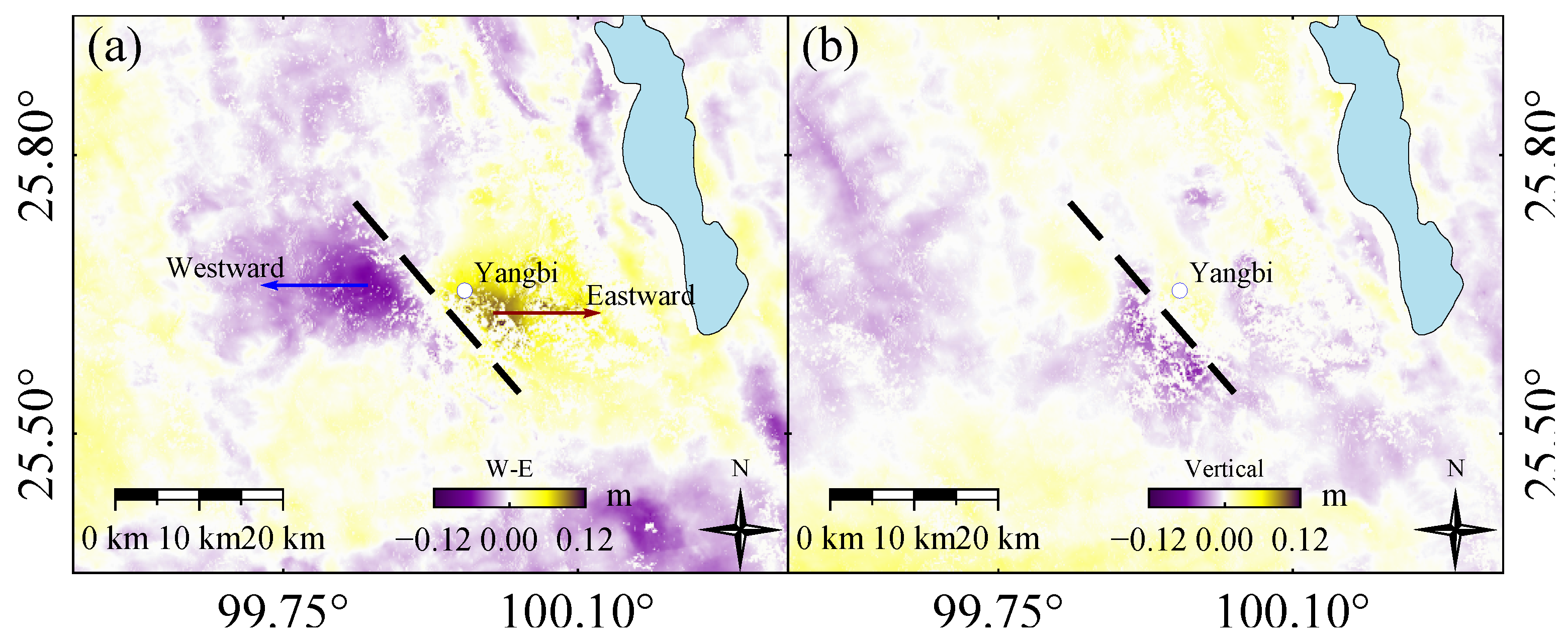
3.2. 2.5-D Surface Deformation
3.3. Source Modeling Method
3.4. Calculation of Coulomb Failure Stress Changes
3.5. Simulation of Strong Ground Motion
4. Results
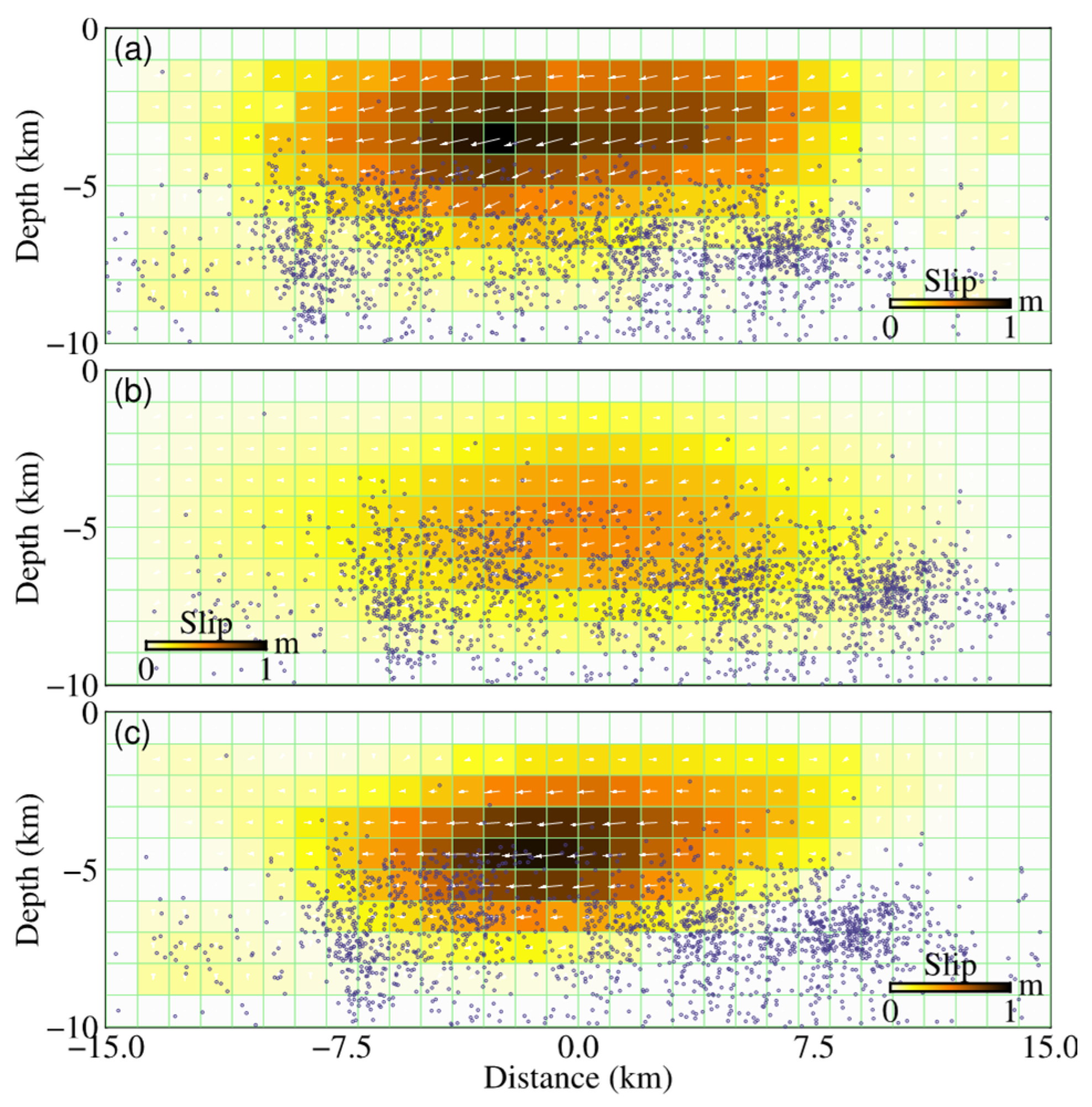
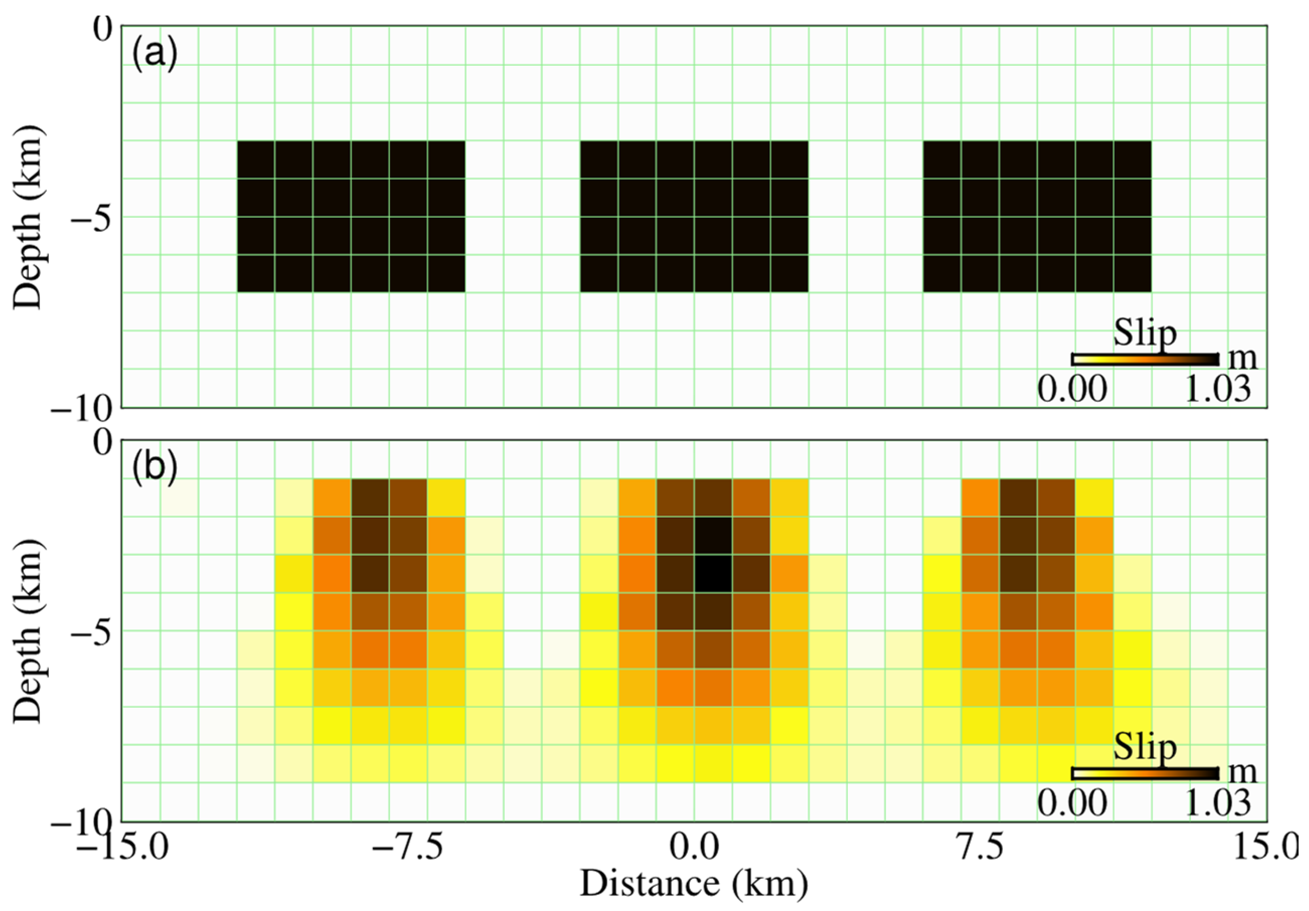
4.1. Source Model
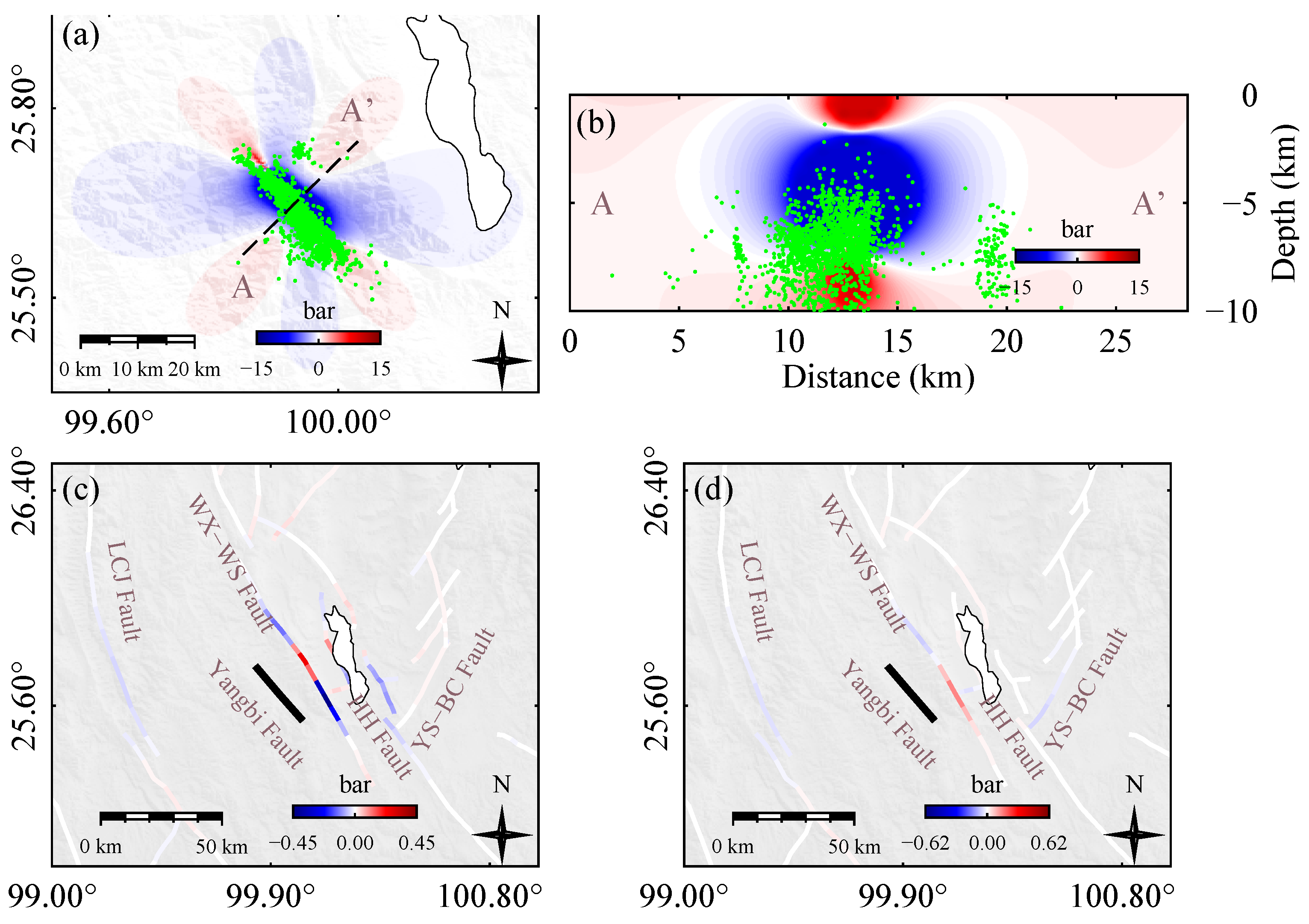
4.2. CFS Change
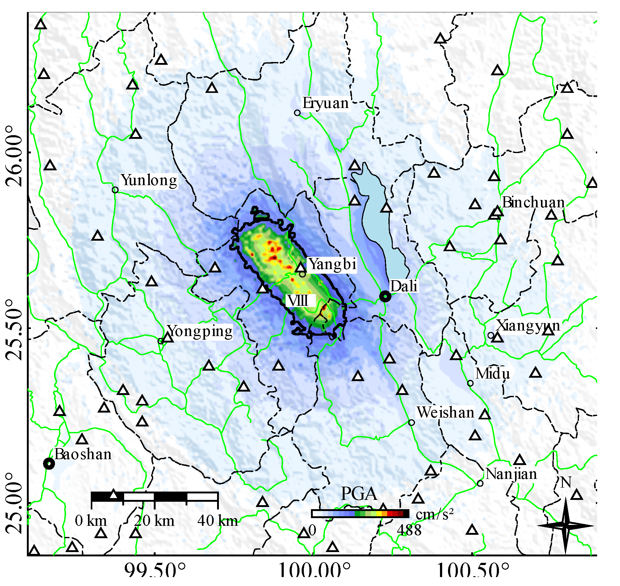
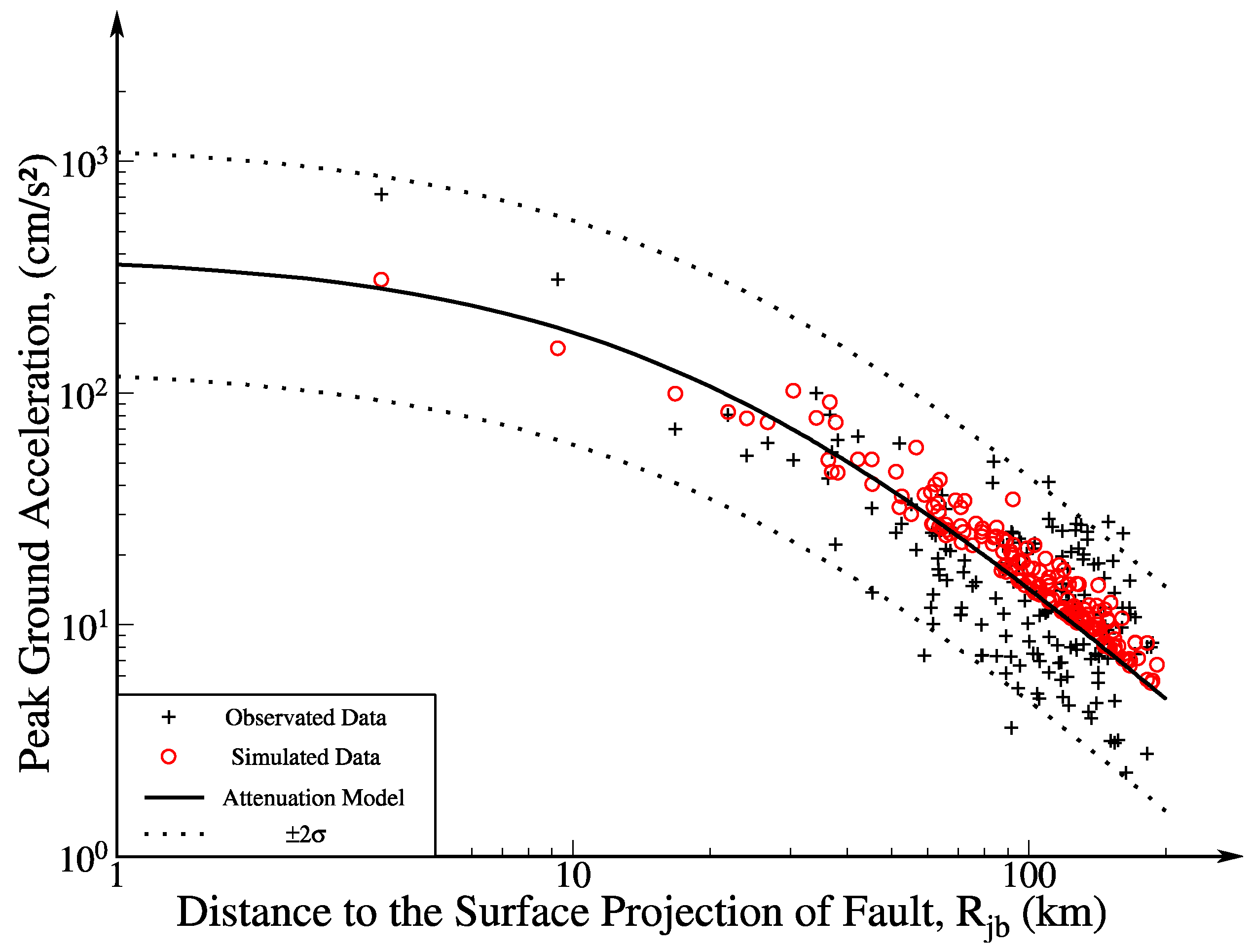
4.3. Peak Ground Acceleration (PGA)
5. Discussion
6. Conclusions
Supplementary Materials
Author Contributions
Funding
Institutional Review Board Statement
Informed Consent Statement
Data Availability Statement
Acknowledgments
Conflicts of Interest
References
- Yang, T.; Li, B.; Fang, L.; Su, Y.; Zhong, Y.; Yang, J.; Qin, M.; Xu, Y. Relocation of the Foreshocks and Aftershocks of the 2021 Ms6.4 Yangbi Earthquake. 2021. Available online: https://www.researchgate.net/profile/Lihua-Fang-3/publication/352441845_Relocation_of_the_foreshocks_and_aftershocks_of_the_2021_Ms64_Yangbi_earthquake/links/60c9edfa299bf1cd71d160d9/Relocation-of-the-foreshocks-and-aftershocks-of-the-2021-Ms64-Yangbi-earthquake.pdf (accessed on 14 October 2021).
- Lei, X.; Wang, Z.; Ma, S.; He, C. A preliminary study on the characteristics and mechanism of the May 2021 MS6.4, Yangbi earthquake sequence, Yunnan, China. Acta Seismol. Sin. 2021, 43, 261–286. (In Chinese) [Google Scholar] [CrossRef]
- Khoshmanesh, M.; Shirzaei, M. Multiscale Dynamics of Aseismic Slip on Central San Andreas Fault. Geophys. Res. Lett. 2018, 45, 2274–2282. [Google Scholar] [CrossRef]
- Wang, H.; Wright, T.J.; Liu-Zeng, J.; Peng, L. Strain Rate Distribution in South-Central Tibet From Two Decades of InSAR and GPS. Geophys. Res. Lett. 2019, 46, 5170–5179. [Google Scholar] [CrossRef] [Green Version]
- Song, X.; Jiang, Y.; Shan, X.; Gong, W.; Qu, C. A Fine Velocity and Strain Rate Field of Present-Day Crustal Motion of the Northeastern Tibetan Plateau Inverted Jointly by InSAR and GPS. Remote Sens. 2019, 11, 435. [Google Scholar] [CrossRef] [Green Version]
- Morishita, Y.; Lazecky, M.; Wright, T.J.; Weiss, J.R.; Elliott, J.R.; Hooper, A. LiCSBAS: An Open-Source InSAR Time Series Analysis Package Integrated with the LiCSAR Automated Sentinel-1 InSAR Processor. Remote Sens. 2020, 12, 424. [Google Scholar] [CrossRef] [Green Version]
- Xu, W.; Wu, S.; Materna, K.; Nadeau, R.; Floyd, M.; Funning, G.; Chaussard, E.; Johnson, C.W.; Murray, J.R.; Ding, X.; et al. Interseismic Ground Deformation and Fault Slip Rates in the Greater San Francisco Bay Area From Two Decades of Space Geodetic Data. J. Geophys. Res. Solid Earth 2018, 123, 8095–8109. [Google Scholar] [CrossRef]
- Jónsson, S.; Zebker, H.; Segall, P.; Amelung, F. Fault Slip Distribution of the 1999 Mw 7.1 Hector Mine, California Earthquake, Estimated from Satellite Radar and GPS Measurements. Bull. Seism. Soc. Am. 2002, 92, 1377–1389. [Google Scholar] [CrossRef]
- Sun, J.; Shen, Z.K.; Bürgmann, R.; Xu, X. Coseismic Slip Distribution of the 24 March 2011 Tarlay (Myanmar) Mw 6.8 Earthquake from ALOS PALSAR Interferometry. Bull. Seismol. Soc. Am. 2013, 103, 2928–2936. [Google Scholar] [CrossRef]
- Zhao, D.; Qu, C.; Shan, X.; Bürgmann, R.; Gong, W.; Tung, H.; Zhang, G.; Song, X.; Qiao, X. Multifault complex rupture and afterslip associated with the 2018 Mw 6.4 Hualien earthquake in northeastern Taiwan. Geophys. J. Int. 2021, 224, 416–434. [Google Scholar] [CrossRef]
- Li, C.; Zhang, G.; Shan, X.; Zhao, D.; Song, X. Geometric Variation in the Surface Rupture of the 2018 Mw7.5 Palu Earthquake from Subpixel Optical Image Correlation. Remote Sens. 2020, 12, 3436. [Google Scholar] [CrossRef]
- Yang, Y.; Chen, Q.; Xu, Q.; Liu, G.; Hu, J.-C. Source model and Coulomb stress change of the 2015 Mw 7.8 Gorkha earthquake determined from improved inversion of geodetic surface deformation observations. J. Geod. 2018, 93, 333–351. [Google Scholar] [CrossRef]
- Wang, K.; Bürgmann, R. Co- and Early Postseismic Deformation Due to the 2019 Ridgecrest Earthquake Sequence Constrained by Sentinel-1 and COSMO-SkyMed SAR Data. Seismol. Res. Lett. 2020, 91, 1998–2009. [Google Scholar] [CrossRef]
- Motagh, M.; Beavan, J.; Fielding, E.J.; Haghshenas, M. Postseismic Ground Deformation Following the September 2010 Darfield, New Zealand, Earthquake From TerraSAR-X, COSMO-SkyMed, and ALOS InSAR. IEEE Geosci. Remote Sens. Lett. 2014, 11, 186–190. [Google Scholar] [CrossRef]
- Fathian, A.; Atzori, S.; Nazari, H.; Reicherter, K.; Salvi, S.; Svigkas, N.; Tatar, M.; Tolomei, C.; Yaminifard, F. Complex co- and postseismic faulting of the 2017–2018 seismic sequence in western Iran revealed by InSAR and seismic data. Remote Sens. Environ. 2021, 253, 112224. [Google Scholar] [CrossRef]
- Yue, H.; Ross, Z.E.; Liang, C.; Michel, S.; Fattahi, H.; Fielding, E.; Moore, A.; Liu, Z.; Jia, B. The 2016 Kumamoto Mw = 7.0 earthquake: A significant event in a fault-volcano system. J. Geophys. Res. Solid Earth 2017, 122, 9166–9183. [Google Scholar] [CrossRef]
- Wen, Y.; Xiao, Z.; He, P.; Zang, J.; Liu, Y.; Xu, C. Source Characteristics of the 2020 Mw 7.4 Oaxaca, Mexico, Earthquake Estimated from GPS, InSAR, and Teleseismic Waveforms. Seismol. Res. Lett. 2021, 92, 1900–1912. [Google Scholar] [CrossRef]
- Zhang, K.; Gan, W.; Liang, S.; Xiao, G.; Dai, C.; Wang, Y.; Li, C.; Zhang, L.; Ma, G. Coseismic displacement and slip distribution of the 2021 May 21, MS6.4, Yangbi Earthquake derived from GNSS observations. Chin. J. Geophys. 2021, 64, 14. (In Chinese) [Google Scholar] [CrossRef]
- Wang, S.; Liu, Y.; Shan, X.; Qu, C.; Zhang, G.; Xie, C.; Zhao, D.; Fan, X.; Hua, J.; Liang, S.; et al. Coseismic surface deformation and slip models of the 2021 Ms6.4 Yangbi (Yunnan, China) earthquake. Seismol. Geol. 2021, 43, 14. (In Chinese) [Google Scholar] [CrossRef]
- Wu, D.; Deng, Q. Basic Characteristics of the Rift Basin in Northwestern Yunnan; Seismological Press: Beijing, China, 1985. [Google Scholar]
- Aydin, A.; Nur, A. Evolution of pull-apart basins and their scale independence. Tectonics 1982, 1, 15. [Google Scholar] [CrossRef]
- Smit, J.; Brun, J.P.; Cloetingh, S.; Ben-Avraham, Z. Pull-apart basin formation and development in narrow transform zones with application to the Dead Sea Basin. Tectonics 2008, 27, TC6018. [Google Scholar] [CrossRef] [Green Version]
- He, X.; Zhao, L.F.; Xie, X.B.; Tian, X.; Yao, Z.X. Weak Crust in Southeast Tibetan Plateau Revealed by Lg-Wave Attenuation Tomography: Implications for Crustal Material Escape. J. Geophys. Res. Solid Earth 2021, 126, 1–17. [Google Scholar] [CrossRef]
- Liu, J.; Ji, C.; Zhang, J.; Zhang, P.; Zeng, L.; Li, Z.; Wang, W. Tectonic setting and general features of coseismic rupture of the 25 April, 2015 Mw 7.8 Gorkha, Nepal earthquake. Chin. Sci. Bull. 2015, 60, 2640–2655. [Google Scholar] [CrossRef] [Green Version]
- Xuan, S.; Shen, C.; Shen, W.; Wang, J.; Li, J. Crustal structure of the southeastern Tibetan Plateau from gravity data: New evidence for clockwise movement of the Chuan–Dian rhombic block. J. Asian Earth Sci. 2018, 159, 98–108. [Google Scholar] [CrossRef]
- Tapponnier, P.; Zhiqin, X.; Roger, F.; Meyer, B.; Arnaud, N.; Wittlinger, G.; Jingsui, Y. Oblique stepwise rise and growth of the Tibet plateau. Science 2001, 294, 1671–1677. [Google Scholar] [CrossRef] [PubMed]
- Clark, M.K.; Royden, L.H. Topographic ooze: Building the eastern margin of Tibet by lower crustal flow. Geology 2000, 28, 703–706. [Google Scholar] [CrossRef]
- Deng, Q.; Zhang, P.; Ran, Y.; Yang, X.; Min, W.; Chu, Q. Basic characteristics of active tectonics of China. Sci. China Ser. D Earth Sci. 2003, 46, 356–372. (In Chinese) [Google Scholar] [CrossRef]
- Tang, P. Activity of the Weishan Basin Segment of the Weixi-Qiaohou Fault; Yunnan University: Kungming, China, 2013. [Google Scholar]
- Chang, Z.; Chang, H.; Zang, Y.; Dai, B. Recent active features of Weixi-Qiaohou fault and its relationship with the Honghe fault. J. Geomech. 2016, 22, 517–530. (In Chinese) [Google Scholar]
- Valerio, E.; Manzo, M.; Casu, F.; Convertito, V.; De Luca, C.; Manunta, M.; Monterroso, F.; Lanari, R.; De Novellis, V. Seismogenic Source Model of the 2019, Mw 5.9, East-Azerbaijan Earthquake (NW Iran) through the Inversion of Sentinel-1 DInSAR Measurements. Remote Sens. 2020, 12, 1346. [Google Scholar] [CrossRef] [Green Version]
- Sandwell, D.; Mellors, R.; Tong, X.; Wei, M.; Wessel, P. Open radar interferometry software for mapping surface Deformation. EOS Trans. Am. Geophys. Union 2011, 92, 234. [Google Scholar] [CrossRef] [Green Version]
- Sandwell, D.; Mellors, R.; Tong, X.; Wei, M.; Wessel, P. GMTSAR: An InSAR processing system based on generic mapping tools. Scripps Inst. Oceanogr. 2011, 58, 1090004. [Google Scholar] [CrossRef] [Green Version]
- Wang, K.; Fialko, Y. Observations and Modeling of Coseismic and Postseismic Deformation Due To the 2015 Mw 7.8 Gorkha (Nepal) Earthquake. J. Geophys. Res. Solid Earth 2018, 123, 761–779. [Google Scholar] [CrossRef]
- Wang, H.; Liuzeng, J.; Ng, A.H.M.; Ge, L.; Javed, F.; Long, F.; Aoudia, A.; Feng, J.; Shao, Z. Sentinel-1 observations of the 2016 Menyuan earthquake: A buried reverse event linked to the left-lateral Haiyuan fault. Int. J. Appl. Earth Obs. Geoinf. 2017, 61, 14–21. [Google Scholar] [CrossRef]
- Farr, T.G.; Caro, E.; Crippen, R.; Duren, R.; Hensley, S.; Kobrick, M.; Paller, M.; Rodriguez, E.; Rosen, L.R.; Seal, D.; et al. The Shuttle Radar Topography Mission. Rev. Geophys. 2007, 45, 183. [Google Scholar] [CrossRef] [Green Version]
- Baran, I.; Stewart, M.P.; Kampes, B.M.; Perski, Z.; Lilly, P. A modification to the Goldstein Radar Interferogram Filter. IEEE Trans. Geosci. Remote Sens. 2003, 41, 2114–2118. [Google Scholar] [CrossRef] [Green Version]
- Chen, C.W.; Zebker, H.A. Network approaches to two-dimensional phase unwrapping: Intractability and two new algorithms. J. Opt. Soc. Am. A-Opt. Image Sci. Vis. 2001, 17, 401–414. [Google Scholar] [CrossRef] [PubMed]
- Li, Z.; Xu, W.; Feng, G.; Hu, J.; Wang, C.; Ding, X.; Zhu, J. Correcting atmospheric effects on InSAR with MERIS water vapour data and elevation-dependent interpolation model. Geophys. J. Int. 2012, 189, 898–910. [Google Scholar] [CrossRef] [Green Version]
- He, P.; Wen, Y.; Ding, K.; Xu, C. Normal Faulting in the 2020 Mw 6.2 Yutian Event: Implications for Ongoing E–W Thinning in Northern Tibet. Remote Sens. 2020, 12, 3012. [Google Scholar] [CrossRef]
- Yu, C.; Li, Z.; Chen, J.; Hu, J.-C. Small Magnitude Co-Seismic Deformation of the 2017 Mw 6.4 Nyingchi Earthquake Revealed by InSAR Measurements with Atmospheric Correction. Remote Sens. 2018, 10, 684. [Google Scholar] [CrossRef] [Green Version]
- Yu, C.; Penna, N.T.; Li, Z. Generation of real-time mode high-resolution water vapor fields from GPS observations. J. Geophys. Res. Atmos. 2017, 122, 2008–2025. [Google Scholar] [CrossRef]
- Yu, C.; Li, Z.; Penna, N.T.; Crippa, P. Generic Atmospheric Correction Model for Interferometric Synthetic Aperture Radar Observations. J. Geophys. Res. Solid Earth 2018, 123, 9202–9222. [Google Scholar] [CrossRef]
- Feng, G.; Li, Z.; Xu, B.; Shan, X.; Zhang, L.; Zhu, J. Coseismic Deformation of the 2015 Mw 6.4 Pishan, China, Earthquake Estimated from Sentinel-1A and ALOS2 Data. Seismol. Res. Lett. 2016, 87, 800–806. [Google Scholar] [CrossRef]
- Yang, Y.; Zhu, J.; Wang, Y.; Xu, B. 3D displacement field of 2016 Kaohsiung Ms 6.7 earthquake from D-InSAR and along-track interferometry with ascending and descending Sentinel-1 images. J. Geod. Geodyn. 2017, 37, 5. (In Chinese) [Google Scholar] [CrossRef]
- Hanssen, R. Radar Interferometry: Data Interpretation and Error Analysis; Kluwer: Dordrecht, The Netherlands, 2001. [Google Scholar]
- Wright, T.J.; Parsons, B.E.; Lu, Z. Toward mapping surface deformation in three dimensions using InSAR. Geophys. Res. Lett. 2004, 31, L01607. [Google Scholar] [CrossRef] [Green Version]
- Wang, Y.; Li, Z.; Zhu, J.; Hu, J. Coseismic three-dimensional deformation of L’Aquila earthquake derived from multi-platform DInSAR data. Geomat. Inf. Sci. Wuhan Univ. 2012, 37, 859–863. [Google Scholar]
- Fujiwara, S.; Nishimura, T.; Murakami, M.; Nakagawa, H.; Tobita, M.; Rosen, P.A. 2.5-D surface deformation of M6.1 earthquake near Mt Iwate detected by SAR interferometry. Geophys. Res. Lett. 2000, 27, 2049–2052. [Google Scholar] [CrossRef]
- Okada, Y. Surface deformation due to shear and tensile faults in a half-space. Bull. Seismol. Soc. Am. 1985, 75, 1135–1154. [Google Scholar] [CrossRef]
- Feng, W.; Tian, Y.; Zhang, Y.; Samsonov, S.; Almeida, R.; Liu, P. A Slip Gap of the 2016 Mw 6.6 Muji, Xinjiang, China, Earthquake Inferred from Sentinel-1 TOPS Interferometry. Seismol. Res. Lett. 2017, 88, 1054–1064. [Google Scholar] [CrossRef]
- Bagnardi, M.; Hooper, A. Inversion of Surface Deformation Data for Rapid Estimates of Source Parameters and Uncertainties: A Bayesian Approach. Geochem.Geophys. Geosyst. 2018, 19, 2194–2211. [Google Scholar] [CrossRef]
- Wright, T.J.; Lu, Z.; Wicks, C. Source model for the Mw 6.7, 23 October 2002, Nenana Mountain Earthquake (Alaska) from InSAR. Geophys. Res. Lett. 2003, 30, 1974. [Google Scholar] [CrossRef]
- Toda, S.; Stein, R.S.; Beroza, G.C.; Marsan, D. Aftershocks halted by static stress shadows. Nature Geosci. 2012, 5, 410–413. [Google Scholar] [CrossRef]
- Harris, R.A. Introduction to special section: Stress triggers, stress shadows, and implications for seismic hazard. J. Geophys. Res. 1998, 103, 22. [Google Scholar] [CrossRef]
- Toda, S.; Matsumura, S. Spatio-temporal stress states estimated from seismicity rate changes in the Tokai region, central Japan. Tectonophysics 2006, 417, 53–68. [Google Scholar] [CrossRef]
- Hardebeck, J.L.; Nazareth, J.J.; Hauksson, E. The static stress change triggering model: Constraints from two southern California aftershock sequences. J. Geophys. Res. Solid Earth 1998, 103, 24427–24437. [Google Scholar] [CrossRef] [Green Version]
- Wang, S.; Yu, Y.; Gao, A.; Yan, X. Development of attenuation relations for ground motion in China. Earthq. Res. China 2000, 16, 8. (In Chinese) [Google Scholar]
- Chen, K.; Yu, Y.; Gao, M. Research on Shakemap system in terms of the site effect. Earthq. Res. China 2010, 26, 11. (In Chinese) [Google Scholar]
- Allen, T.I.; Wald, D.J. Topographic Slope as a Proxy for Seismic Site-Conditions (VS30) and Amplification Around the Globe; Open-File Report 2007-1357; U.S. Geological Survey: Reston, VA, USA, 2007.
- Heath, D.C.; Wald, D.J.; Worden, C.B.; Thompson, E.M.; Smoczyk, G.M. A global hybrid V S 30 map with a topographic slope–based default and regional map insets. Earthq. Spectra 2020, 36, 1570–1584. [Google Scholar] [CrossRef]
- Avouac, J.P.; Meng, L.; Wei, S.; Wang, T.; Ampuero, J.P. Lower edge of locked Main Himalayan Thrust unzipped by the 2015 Gorkha earthquake. Nat. Geosci. 2015, 8, 708–711. [Google Scholar] [CrossRef] [Green Version]
- Melgar, D.; Fan, W.; Riquelme, S.; Geng, J.; Liang, C.; Fuentes, M.; Vargas, G.; Allen, R.M.; Shearer, P.M.; Fielding, E.J. Slip segmentation and slow rupture to the trench during the 2015, Mw 8.3 Illapel, Chile earthquake. Geophys. Res. Lett. 2016, 43, 961–966. [Google Scholar] [CrossRef]
- Li, Y.; Xu, X.; Zhang, E.; Gao, J. Three-dimensional crust structure beneath SE Tibetan Plateau and its seismotectonic implications for the Ludian and Jinggu earthquakes. Seismol. Geol. 2014, 36, 13. (In Chinese) [Google Scholar] [CrossRef]
- Zeng, Z.; Fan, G. Structural Geology; China University of Geosciences Press: Wuhan, China, 2020. [Google Scholar]
- Zhang, K.; Liang, S.; Gan, W. Crustal strain rates of southeastern Tibetan plateau derived from GPS measurements and implications to lithospheric deformation of the Shan-Thai terrane. Earth Planet. Phys. 2019, 3, 1–8. [Google Scholar] [CrossRef]
- Schoenbohm, L.M.; Burchfiel, B.C.; Liangzhong, C.; Jiyun, Y. Miocene to present activity along the Red River fault, China, in the context of continental extrusion, upper-crustal rotation, and lower-crustal flow. GSA Bull. 2006, 118, 672–688. [Google Scholar] [CrossRef]
- Chen, K.; Yu, Y.; Gao, M.; Feng, J. Study on bias correction of ShakeMaps based on limited acceleration records. Acta Seismol. Sin. 2012, 34, 633–645. (In Chinese) [Google Scholar]
- Worden, C.B.; Wald, D.J.; Allen, T.I.; Lin, K.; Garcia, D.; Cua, G. A Revised Ground-Motion and Intensity Interpolation Scheme for ShakeMap. Bull. Seismol. Soc. Am. 2010, 100, 3083–3096. [Google Scholar] [CrossRef]
- Zhong, S.; Xu, C.; Yi, L.; Li, Y. Focal Mechanisms of the 2016 Central Italy Earthquake Sequence Inferred from High-Rate GPS and Broadband Seismic Waveforms. Remote Sens. 2018, 10, 512. [Google Scholar] [CrossRef] [Green Version]
- Kawamoto, S.; Ohta, Y.; Hiyama, Y.; Todoriki, M.; Nishimura, T.; Furuya, T.; Sato, Y.; Yahagi, T.; Miyagawa, K. REGARD: A new GNSS-based real-time finite fault modeling system for GEONET. J. Geophys. Res. 2017, 122, 1324–1349. [Google Scholar] [CrossRef]
- Cheloni, D.; Akinci, A. Source modelling and strong ground motion simulations for the 24 January 2020, Mw 6.8 Elazığ earthquake, Turkey. Geophys. J. Int. 2020, 223, 1054–1068. [Google Scholar] [CrossRef]
- Wessel, P.; Smith, W.H.F. New, improved version of generic mapping tools released. EOS Trans. Am. Geophys. Union 1998, 79, 579. [Google Scholar] [CrossRef]


| Sensor | Acquisition Time (M-D-Y) | Orbit Direction | Path Number | Frame Number | Heading Angle (°) |
|---|---|---|---|---|---|
| Sentinel-1A | 20 May 2021 | Ascending | 99 | 1265 | −12.5 |
| Sentinel-1B | 26 May 2021 | ||||
| Sentinel-1A | 10 May 2021 | Descending | 135 | 508 | −167.5 |
| Sentinel-1A | 22 May 2021 |
Publisher’s Note: MDPI stays neutral with regard to jurisdictional claims in published maps and institutional affiliations. |
© 2021 by the authors. Licensee MDPI, Basel, Switzerland. This article is an open access article distributed under the terms and conditions of the Creative Commons Attribution (CC BY) license (https://creativecommons.org/licenses/by/4.0/).
Share and Cite
Wang, Y.; Chen, K.; Shi, Y.; Zhang, X.; Chen, S.; Li, P.; Lu, D. Source Model and Simulated Strong Ground Motion of the 2021 Yangbi, China Shallow Earthquake Constrained by InSAR Observations. Remote Sens. 2021, 13, 4138. https://0-doi-org.brum.beds.ac.uk/10.3390/rs13204138
Wang Y, Chen K, Shi Y, Zhang X, Chen S, Li P, Lu D. Source Model and Simulated Strong Ground Motion of the 2021 Yangbi, China Shallow Earthquake Constrained by InSAR Observations. Remote Sensing. 2021; 13(20):4138. https://0-doi-org.brum.beds.ac.uk/10.3390/rs13204138
Chicago/Turabian StyleWang, Yongzhe, Kun Chen, Ying Shi, Xu Zhang, Shi Chen, Ping’en Li, and Donghua Lu. 2021. "Source Model and Simulated Strong Ground Motion of the 2021 Yangbi, China Shallow Earthquake Constrained by InSAR Observations" Remote Sensing 13, no. 20: 4138. https://0-doi-org.brum.beds.ac.uk/10.3390/rs13204138