
MADNet 2.0: Pixel-Scale Topography Retrieval from Single-View Orbital Imagery of Mars Using Deep Learning


1
Mullard Space Science Laboratory, Imaging Group, Department of Space and Climate Physics, University College London, Holmbury St Mary, Surrey RH5 6NT, UK
2
College of Civil and Transportation Engineering, Shenzhen University, Shenzhen 518060, China
3
Ministry of Natural Resources Key Laboratory for Geo-Environmental Monitoring of Great Bay Area & Guangdong Key Laboratory of Urban Informatics & Shenzhen Key Laboratory of Spatial Smart Sensing and Services, Shenzhen University, Shenzhen 518060, China
4
Laboratoire de Planétologie et Géodynamique, CNRS, UMR 6112, Universités de Nantes, 44300 Nantes, France
*
Author to whom correspondence should be addressed.
Remote Sens. 2021, 13(21), 4220; https://0-doi-org.brum.beds.ac.uk/10.3390/rs13214220
Submission received: 23 September 2021
/
Revised: 18 October 2021
/
Accepted: 19 October 2021
/
Published: 21 October 2021
(This article belongs to the Special Issue Mars Remote Sensing)
Abstract
:The High-Resolution Imaging Science Experiment (HiRISE) onboard the Mars Reconnaissance Orbiter provides remotely sensed imagery at the highest spatial resolution at 25–50 cm/pixel of the surface of Mars. However, due to the spatial resolution being so high, the total area covered by HiRISE targeted stereo acquisitions is very limited. This results in a lack of the availability of high-resolution digital terrain models (DTMs) which are better than 1 m/pixel. Such high-resolution DTMs have always been considered desirable for the international community of planetary scientists to carry out fine-scale geological analysis of the Martian surface. Recently, new deep learning-based techniques that are able to retrieve DTMs from single optical orbital imagery have been developed and applied to single HiRISE observational data. In this paper, we improve upon a previously developed single-image DTM estimation system called MADNet (1.0). We propose optimisations which we collectively call MADNet 2.0, which is based on a supervised image-to-height estimation network, multi-scale DTM reconstruction, and 3D co-alignment processes. In particular, we employ optimised single-scale inference and multi-scale reconstruction (in MADNet 2.0), instead of multi-scale inference and single-scale reconstruction (in MADNet 1.0), to produce more accurate large-scale topographic retrieval with boosted fine-scale resolution. We demonstrate the improvements of the MADNet 2.0 DTMs produced using HiRISE images, in comparison to the MADNet 1.0 DTMs and the published Planetary Data System (PDS) DTMs over the ExoMars Rosalind Franklin rover’s landing site at Oxia Planum. Qualitative and quantitative assessments suggest the proposed MADNet 2.0 system is capable of producing pixel-scale DTM retrieval at the same spatial resolution (25 cm/pixel) of the input HiRISE images.
Keywords:
3D mapping; digital terrain model; DTM; topography; small-scale; high-resolution; Mars; deep learning; HiRISE; HRSC; ExoMars; Oxia Planum1. Introduction
High-resolution digital terrain models (DTMs) have always been considered as a key geospatial data product for studying a planetary surface such as Mars. For example, DTMs derived from the Mars Express’s 12.5–25 m/pixel High-Resolution Stereo Camera (HRSC) [1] are able to provide topographic context of a large area, whilst DTMs derived from the Mars Reconnaissance Orbiter (MRO) 6 m/pixel Context Camera (CTX) [2] and the ExoMars Trace Gas Orbiter (TGO) 4–6 m/pixel Colour and Stereo Surface Imaging System (CaSSIS) [3] allow us to study moderately finer scale topography at the decametre-scale. Moreover, for a small percentage of the Martian surface, DTMs derived from the MRO 25–50 cm/pixel High-Resolution Imaging Science Experiment (HiRISE) [4] targeted stereo acquisitions are able to reveal detailed topographic information of surface features or processes at metre-scale. The high-resolution DTMs from HiRISE have become an invaluable resource for the international community of planetary scientists to carry out geological analysis of the Martian landscapes.
However, due to the spatial resolution being very high, the surface coverage of HiRISE observations is rather limited. According to the product coverage shapefile (https://ode.rsl.wustl.edu/mars/coverage/ODE_Mars_shapefile.html, accessed on 15 October 2021) released on 2 September 2021, the existing HiRISE images have a total coverage of 3.405% of the Martian surface (see Figure 1). The total coverage of HiRISE targeted stereo acquisitions is lower—currently being 0.316%. This means with traditional photogrammetric methods, only 0.316% of the Martian surface can possibly be mapped into 3D at a high- resolution of about 1 m/pixel. For example, the publicly available NASA Planetary Data System (PDS) 1–2 m/pixel HiRISE DTMs (https://www.uahirise.org/dtm/, accessed on 15 October 2021) currently have a total surface coverage of 0.0297%. However, deep learning-based techniques have recently been developed that are able to retrieve DTMs using only a single HiRISE observation as input [5,6,7]. Using deep learning-based single-image DTM retrieval methods, ultra-high-resolution (25–50 cm/pixel) 3D information can now be derived “on-demand” for the remaining 3.098% area of the Martian surface, in which case, meaning scientific analysis that is reliant on high-resolution 3D will become feasible in these remaining areas.
In this work, we build on our previous development of the Multi-scale Generative Adversarial U-Net based single-image DTM estimation system (MADNet; hereafter referred to as MADNet 1.0) [6] and propose several key modifications to the original network architecture and the processing pipeline to improve the results and to resolve the issues that are summarised in Section 2.1 of this paper. We propose the new MADNet 2.0 system that employs a simplified and optimised single-image DTM estimation network for pixel-scale DTM retrieval together with a coarse-to-fine reconstruction scheme on top of the DTM inference process. A new set of training data is constructed using selected PDS HiRISE DTMs and iMars CTX DTMs [8] which are available through the ESA’s Guest Storage Facility [9] (https://www.cosmos.esa.int/web/psa/ucl-mssl_meta-gsf, accessed on 15 October 2021). We demonstrate the new MADNet 2.0 system with single-view HiRISE images over the ExoMars Rosalind Franklin rover’s landing site at Oxia Planum [7,10]. The HRSC and CTX DTM mosaics over the same area (described in [7]) that are co-aligned with the Mars Global Surveyor’s Mars Orbiter Laser Altimeter (MOLA) [11,12] global areoid DTM (https://planetarymaps.usgs.gov/mosaic/Mars_MGS_MOLA_DEM_mosaic_global_463m.tif, accessed on 15 October 2021), are used as the baseline reference data. Qualitative assessments using colourised and shaded relief DTMs, and quantitative assessments using semi-automated crater size-counting, and automated slanted-edge image sharpness measurements, are provided for the resultant MADNet 2.0 DTMs, in comparison with the PDS HiRISE DTMs and the MADNet 1.0 HiRISE DTM mosaic product that was produced and described in [7]. In addition, DTM profile and difference measurements are performed for sub-areas to show the height accuracy of the resultant MADNet 2.0 HiRISE DTMs, in comparison with the PDS HiRISE DTMs and the reference CTX DTM.
MADNet 2.0 resolves major issues of the MADNet 1.0 system and produces high-quality topography retrieval at the same spatial resolution of the input image (i.e., pixel-scale topography retrieval). Figure 2 shows an example of side-by-side comparisons of one of the 25 cm/pixel input HiRISE images, the 1 m/pixel PDS DTM, the 50 cm/pixel MADNet 1.0 DTM, and the 25 cm/pixel DTM that is produced by the proposed MADNet 2.0 single-image DTM estimation system.
The layout of the rest of the paper is as follows. In Section 1.1, we review previous work in the field of single-image deep learning-based height/depth estimation. In Section 2.1, we summarise the overall workflow and key remaining issues with the MADNet 1.0 system. This is followed by a discussion of the proposed changes and justifications for the MADNet 2.0 system in Section 2.2 and network training details in Section 2.3. In Section 2.4, we introduce the datasets and the experiments. Results are qualitatively demonstrated in Section 3.1 and quantitative assessments are provided in Section 3.2 and in Section 3.3 where we present profile and DTM difference measurements. In Section 4.1, we demonstrate the extensibility of the MADNet 2.0 system using a single HRSC image and the MOLA DTM as inputs to produce a high-quality pixel-scale HRSC DTM. This is followed by a brief discussion of the remaining limitations and future work in Section 4.2 before the conclusions are drawn in Section 5.
1.1. Previous Work
Although photogrammetry and multi-view stereo have a long history in the field of computer vision, height or depth from a single-view image (excluding traditional photoclinometry [13,14,15]) only started being considered feasible in recent years, alongside the great success of the development of deep learning techniques, wherein the term for single-image DTM/height/depth estimation is generally referred to as “monocular depth estimation” (MDE). With a variety of potential applications in the fields of robotics, autonomous driving, virtual reality, and etc., several hundreds of MDE methods/networks have been proposed [16,17,18,19] over the last 7 years. In terms of training mechanisms, these MDE methods can be classified into supervised methods, requiring ground truth depth image for training, and unsupervised methods, using 3D geometry and requiring only multi-view images as inputs. For ground-based applications, MDE networks are generally trained with outdoor or indoor scenes [20,21,22] either with ground truth measured by LIDAR (Light Detection and Ranging) for supervised learning or with multi-camera or video inputs for calculation of the underlying 3D geometry for unsupervised learning.
In terms of the supervised methods, the earliest successful experiments of applying convolutional neural networks (CNNs) to address MDE was reported in [23,24], wherein the authors proposed a multi-scale CNN architecture, a scale-invariant mean squared error (MSE) and the gradients of the differences (in horizontal and vertical directions) based loss functions. Following these, fully CNNs and residual networks were proposed in [25,26,27] to address MDE, as well as using the Berhu loss function [28] to improve the efficiency and accuracy of the MDE models. Exploring the continuous characteristics of the neighbouring depth with semantic segmentation, [29,30,31,32] combined CNN with the conditional random field (CRF) models and semantic image segmentation to improve their MDE results. More recently, architectures based on the generative adversarial networks (GAN) [33], the encoder-decoder style U-net [34], and the selective attention-based networks, have all shown positive impacts on resolving MDE. Some of the representative methods of these can be found in [35,36] for GAN-based approaches, in [37,38] for U-net-based approaches, and in [39,40] for selective attention-based approaches.
In terms of the unsupervised methods, early breakthrough work was reported in [41,42], wherein the two groups of authors employed the disparity network and the pose network, to regress the transformations between stereo views (namely, “MDE from stereo consistency”) and between neighbouring continuous frames (namely, “MDE from multi-view”), respectively. Following these, the authors in [43,44], proposed the use of the structural similarity index measurement (SSIM) [45] based appearance loss, the disparity smoothness loss, and the auto-masking loss to overcome a variety of issues caused by using only the photogrammetric loss. For “MDE from stereo consistency”, traditional methods of visual odometry and photogrammetry are typically employed [46,47,48], while on the other hand, optical flow methods are generally employed for “MDE from multi-view” [49,50,51]. Similar to the supervised MDE methods, GANs were also introduced into unsupervised MDE methods, using reconstructed/reprojected views and real views as the inputs for training the discriminator network [52,53,54].
In addition to the above, some other work focused on the topic of “depth completion” [19], which is different but directly relevant to MDE, aiming at improving the quality of the MDE results. These works generally refer to MDE denoising [55,56] and MDE refinement [57,58]. More recently, new depth completion methods, such as depth super-resolution [59,60,61,62] using subpixel convolutional layers, and multi-resolution fusion [63,64] using content-adaptive depth merging networks, have also shown fairly good impacts on MDE, producing high-quality depth maps with effective spatial resolutions that are very close to those of the input images.
In contrast to the ground-based MDE tasks, single-image DTM estimation tasks using Mars orbital imagery [5,6,7] is different in many aspects. Firstly, the sizes of the target input images are different. For example, a HiRISE image (gigapixel) is much larger in size than a typical ground-based input image (megapixel). This results in extra procedures being required for spatial tiling, mosaicing, as well as multi-scale reconstruction to perform single-image DTM estimation tasks. Secondly, the viewpoints are different, resulting in the typical “global depth cues” that are used in MDE, such as linear perspective, object size and occlusion in relation to object position, texture density, atmospheric effects, being limited or non-existent in single-image DTM estimation tasks. Thirdly, the complexity and appearance of objects/features are different. In general, the surface features on Mars orbital imagery are structurally continuous, resulting in a reduced conflict for keeping structural consistency and bringing out high-frequency details. For example, keeping the object border clear and distinctive is always challenging in ground-based MDE tasks, because of the conflicting interests in keeping the large-scale depth continuous (e.g., a scene of a room or road) whilst making the local depth discrete (e.g., around object borders), but this is considered to be a minor issue in single-image DTM estimation tasks for Mars as the topography of the surface is always “continuous”.
2. Materials and Methods
2.1. The MADNet 1.0 System and Summary of Existing Issues
Of particular relevance to this work, we previously proposed the MADNet 1.0 single-image DTM estimation system [6] using supervised learning and multi-resolution 3D co-alignment. The network core is based on a relativistic GAN framework [65,66] with the generator network based on the adaptively weighted multi-scale U-nets [34]. The overall processing chain of the MADNet 1.0 system is illustrated in Figure 3. It takes a co-registered higher resolution image and a lower resolution reference DTM as inputs, and uses image tiling, multi-scale relative height inference, height reconstruction of each tiled inference output, 3D co-alignment with respect to the reference DTM, and DTM tile mosaicing to produce an output DTM at half the resolution of the input image. For multi-scale relative height inference, the MADNet 1.0 generator uses three U-nets in parallel, operating at different image resolutions, each of which contains a stack of the dense convolution blocks (DCBs) [67] and up-projection blocks (UPBs) [27], and are merged with adaptive weights for estimation of a relative height map for each input image tile.
MADNet 1.0 results were demonstrated to be optimal, compared to DTM products processed using major photogrammetric pipelines for HRSC, CTX, CaSSIS, and HiRISE DTM processing, in terms of overall quality and effective resolution, as well as the processing speed [6,7]. However, there are four main issues with the MADNet 1.0 system, which are explained as follows, and demonstrated in detail in Section 3.1 with comparisons with the improved MADNet 2.0 results.
- (a)
- Degraded (or weakened) topographic variation/feature at the intermediate scale between the scales of the input image and reference DTM. This is due to the fact that large-scale (relative to the input image) topographic cues cannot be perceived by the trained model using the small-sized (512 × 512 pixels) tiled input. This missing information may also not be recoverable from the reference DTM if it is not large enough in scale for the lower-resolution reference DTM. This is generally not an issue if we use a reference DTM that has a spatial resolution close to (≤3 times) the resolution of the input image. However, if there is a large resolution gap between the input image and reference DTM, intermediate-scale topographic information of the MADNet 1.0 result is likely to be missing or inaccurate.
- (b)
- Inherited large-scale (relative to the input image) topographic errors or artefacts. Although we should always use a high-quality or pre-corrected DTM as the lower-resolution reference, some small-scale (relative to the reference DTM) errors are inevitable, and consequently, small-scale errors on the lower-resolution reference DTM can potentially become large-scale errors in the higher-resolution output DTM. Building and refining the MADNet 1.0 DTMs progressively using multi-resolution cascaded inputs could minimise the impact of the inherited photogrammetric errors and artefacts [7], but the issue cannot be fully eliminated, and the issue could become more obvious alongside enlarged resolution gap between the input image and reference DTM.
- (c)
- Inconsistent performance (mainly found for high-frequency features) on the DTM inference processes of different tiles of the full-scene input. The effect of this issue is that some of the resultant DTM tiles are sharper and some of the resultant DTM tiles are smoother, and consequently, all these resultant DTM tiles cannot be seamlessly mosaiced together without producing obvious artefacts. Even the smoother ones may still appear to be sharper in comparison to any photogrammetric results, and such issues will still cause discontinuities for local topographic features. Moreover, if there are large and frequent differences in sharpness of adjacent DTM tiles, this creates a patterned gridding artefact on the final DTM result.
- (d)
- Tiling artefacts caused by incorrect or inconsistent inference of large-scale slopes of neighbouring tiles. Due to the memory constraint of a graphics processing unit, the size of the tiled input for inference is limited, and consequently, a large image (e.g., HiRISE) needs to be divided into tens of thousands of tiles. As there are not enough “global height cues” within each input image tile, the predicted large-scale topographic information (e.g., a global slope) is highly likely to be incorrect or inaccurate. 3D fitting and overlapped blending were used in [7] to correct the large-scale error and minimise the impact of the inconsistent large-scale topography of adjacent tiles. However, minor height variations (typically being of the order of ~10 cm) still exist at the joints of neighbouring tiles on steep slopes.
2.2. The Proposed MADNet 2.0 System
In this paper, we propose the MADNet 2.0 single-image DTM estimation system that is based on the MADNet 1.0 system, but with three key modifications to overcome the aforementioned issues and produce pixel-scale DTM retrieval. The flow diagram of the proposed MADNet 2.0 system is shown in Figure 4, highlighting (in yellow) the modifications, in comparison to the MADNet 1.0 system. The three modifications are listed and described as follows.
- (a)
- The coarse-scale and intermediate-scale U-nets of the MADNet 1.0 generator are removed in MADNet 2.0.
There are two reasons for this change. Firstly, as previously explained, global height cues for large-scale features of a large image cannot be perceived by the network with small, tiled inputs, and subsequently, the coarse-scale and intermediate-scale inferences are usually incorrect. Figure 5 shows an example of the inference output from a single tiled input with MADNet 1.0, where the large-scale topography of the raw inference output incorrectly portrays that the high ground is at the bottom of the image. After 3D co-alignment using the reference DTM, the high ground is corrected to the top-left corner of the image. However, even the large-scale topographic information can always be corrected via the subsequent 3D co-alignment process using a reference DTM, the multi-scale approach is considered unstable and rather redundant for the orbital image DTM estimation tasks. Secondly, due to the surface features seen in Mars orbital imagery being structurally continuous, global and local height cues are not necessarily needed to be separately considered. This is different from MDE using perspective views of indoor or outdoor scenes, where local depth cues from occlusions and global depth cues from linear perspectives need to be separately treated. It should be noted that any large-scale height variations (e.g., large-scale slopes that are spatially much bigger than the size of the input tile) are also removed from the training datasets so that more local features can be targeted and learnt by the network (please refer to Section 2.3).
Figure 5 shows the MADNet 1.0 and MADNet 2.0 results from a single input image tile (512 × 512 pixels) of a HiRISE image. We can observe that the aforementioned issue of the large-scale topography of the MADNet 1.0 inference output being incorrect (from bottom to top for high to low) and is not co-aligned with the large-scale topography that is shown in the PDS HiRISE DTM and MADNet 2.0 DTM (from top-left to bottom-right for high to low). Without being constrained by the coarser scale inference introduced by MADNet 1.0, the MADNet 2.0 inference output shows more details of local features. In addition, we can observe from the MADNet 1.0 DTM result that the large-scale topography still does not agree with the MADNet 2.0 DTM and PDS HiRISE DTM, even though all of the three HiRISE DTMs are co-aligned with the same CTX reference DTM using the same method. This is due to the coarse-scale inference of MADNet 1.0 being incorrect, which has a negative impact on the subsequent 3D correction process.
- (b)
- The fine-scale U-net of the MADNet 1.0 generator is optimised, adding an extra block of UPB [27] with concatenation operation at the decoder end, and using the output of each convolution layer (before the pooling layer) of the encoder, instead of using the output of each pooling layer of the encoder, for concatenation with the corresponding output of each UPB of the decoder.
With this proposed network optimisation, MADNet 2.0 is now capable of producing pixel-scale inference, i.e., the output DTM has the same spatial resolution as the input image, instead of being half of the input resolution with MADNet 1.0. The network architecture of MADNet 2.0 is shown in Figure 6. The MADNet 2.0 generator network has an identical structure for its encoder arm with the fine-scale U-net of the MADNet 1.0 generator [6], consisting of a feature extraction layer (7 × 7 kernel, 64 feature maps, stride 2) and a max-pooling layer (3 × 3 kernel, stride 2), followed by a sequence of four DCB [67]—convolution (1 × 1 kernel, stride 1, and with increasing numbers of feature maps of 64, 128, 256, …)—pooling layers (2 × 2 kernel, stride 2), which is then connected to its decoder arm. The decoder arm of the proposed MADNet 2.0 generator network consists of a sequence of five convolution (3 × 3 kernel, stride 1, and with decreasing number of feature maps)—UPB [27]—concatenation (with the corresponding output of each convolution layer from the encoder) layers and followed by a final reconstruction layer (3 × 3 kernel, stride 1). Other than the changes made on the decoder network, we use the same relativistic adversarial training procedure [65,66] and total loss function that is a weighted sum of the gradient loss, Berhu loss [28], and adversarial loss, detailed in [6].
- (c)
- A coarse-to-fine multi-scale reconstruction process is implemented on top of the DTM estimation network.
There are two reasons for adding the coarse-to-fine reconstruction module. Firstly, with the proposed coarse-to-fine reconstruction process, intermediate-scale topographic information, which was reliant on the reference DTM in MADNet 1.0, can now be independently and more accurately retrieved in MADNet 2.0. The MADNet 1.0 system [6] only spatially slices the input image, and consequently, if there is a large resolution gap between the input image and the reference DTM, the intermediate-scale and large-scale topographic information that propagates across multiple DTM tiles could be missing or inaccurate (see Figure 7 for some examples). This is because each individual DTM tile is being predicted independently without being guided by its neighbouring content or global context. It should be noted that the MADNet 1.0 multi-scale reconstruction approach within the DTM estimation network cannot address this issue because it is targeted on a single tile. Secondly, the proposed coarse-to-fine reconstruction process can potentially reduce the inherited artefacts from the reference DTM. With multiple-scale reconstruction, artefacts from the reference DTM can be gradually rectified and their impact on the final fine-scale DTM is therefore weakened through each of the coarser-scale reconstruction processes.
Figure 7 demonstrates the issue of not having the proposed coarse-to-fine reconstruction process; intermediate-scale and large-scale topographic information could be lost or be inaccurate, as such information is solely retrieved from the low-resolution reference DTM in MADNet 1.0. For example, we can observe that even though the small-sized craters are satisfactorily retrieved (indicated with the blue arrows) with MADNet 1.0 (in comparison to the PDS HiRISE DTM), the medium- and large-sized craters appear to be blurred and smooth (indicated with the red arrows) with MADNet 1.0 (in comparison to the PDS HiRISE DTM and MADNet 2.0 results).
In MADNet 2.0, the coarse-to-fine reconstruction module is implemented as follows. Firstly, the input image is downscaled by 16 times and 4 times, then spatially tiled, and each image tile is processed into a DTM tile (inference) using the pre-trained MADNet 2.0 generator. Secondly, all the coarse-scale DTM tiles are corrected (using the same 3D co-alignment method [6,7,68] that is employed in the MADNet 1.0 system) with respect to the input reference DTM and mosaiced together to produce a low-resolution DTM (1/16 times the input image resolution). Thirdly, all the intermediate-scale DTM tiles are corrected with respect to the low-resolution DTM produced at the previous step and mosaiced together to produce an intermediate-resolution DTM (1/4 times the input image resolution). Finally, all the fine-scale DTM tiles are corrected with respect to the intermediate-resolution DTM produced at the previous step and mosaiced together to produce the final high-resolution DTM, having the same resolution as the input image.
2.3. Network Training
The two sets of training data that were used for training of the MADNet 1.0 [6] network consist of 4200 resampled HiRISE ortho-rectified image (ORI) crops (at 4 m/pixel) and DTM crops (at 8 m/pixel) for the first-stage training, and 15,500 resampled HiRISE ORI crops (at 2 m/pixel) and DTM crops (at 4 m/pixel) for the second-stage training. These were formed from 450 publicly available PDS HiRISE DTMs and ORIs, each of which was resampled to match the effective resolution of the photogrammetric DTMs (roughly between 4 m/pixel and 8 m/pixel) and spatially sliced into 512 × 512 pixels (ORI) and 256 × 256 pixels (DTM) crops to match the data dimensions of the network input and output.
As described in Section 2.2, the coarse-scale and intermediate-scale U-nets have been removed in MADNet 2.0, and consequently, the two-stage training process is no longer needed. We have therefore formed a single new training dataset consisting of 4 m/pixel resampled HiRISE ORI and DTM crops, 2 m/pixel resampled HiRISE ORI and DTM crops, and in addition, 36 m/pixel downsampled CTX ORI and DTM crops from the 2300 publicly available iMars (http://www.i-mars.eu/, accessed on 15 October 2021) CTX DTMs and ORIs [8,9] are now included (available at https://www.cosmos.esa.int/web/psa/UCL-MSSL_iMars_CTX_v1.0, accessed on 15 October 2021), all with an identical tile size of 512 × 512 pixels.
In this work, we noticed that even though the HiRISE training datasets used in [6] were roughly screened to remove lower-quality DTMs, there are still about ¼ of them that are either affected by different types of artefacts or lack high-frequency details. We found that not only the quality of each PDS HiRISE DTM is quite varied, but sometimes, different parts of the same image have different DTM quality. The issue of some of the HiRISE DTMs having a lower quality is not necessarily associated with the quality of the corresponding stereo input images, nor does it appear to be related to a certain type of surface feature. We can still observe varied DTM quality (see Figure 8 for examples of these) for the same type of surface feature with similar image quality. Such lower quality training DTM samples prolong the training process and have a negative impact on the accuracy of the inference output.
It should be noted that down-sampling of the training DTMs produced from photogrammetric methods (i.e., PDS HiRISE DTM and iMars CTX DTM sub-image tiles) helps bring their nominal resolution closer to their effective resolution in order to train the network to perform per-pixel image-to-height inference. The down-sampling or averaging process also helps to remove some of the high-frequency photogrammetric artefacts so that we don’t need to remove a training crop that has a few erroneous pixels during screening. The fixed spatial resolutions (2 m/pixel, 4 m/pixel, 36 m/pixel) of the training dataset have a reasonable coverage from high-resolution to low-resolution images of the existing Mars orbital imagers, and we do not observe any differences in the inference performance of test datasets that have different spatial resolutions (e.g., 12.5 m/pixel HRSC images or 25 cm/pixel HiRISE images), according to the HiRISE and HRSC tests of this work, as well as the CaSSIS, CTX, HiRISE tests in the previous work [6,7]. This is the basis for deep learning-based methods to produce better DTMs than using photogrammetric methods, even though photogrammetric DTMs were used for training the model. For instance, after successful training of the down-sampled and screened data, the network has learnt how to produce the best DTM result for an “artefact-free” output for comparably larger-sized features (e.g., craters with diameter larger than 100 m using 4 m/pixel images and DTMs), then the learnt parameter sets can be used to produce the most realistic DTM result for similar features that are much smaller in size (e.g., craters with diameter smaller than 10 m from 0.25 m/pixel images), where many artefacts may appear using photogrammetric methods.
In this work, we further screened the 4 m/pixel and 2 m/pixel HiRISE training samples (total 19,700 ORI-DTM pairs before screening), as well as the 36 m/pixel CTX training samples (total 13,800 ORI-DTM pairs before screening), using the hill-shaded relief samples, which show more qualitative details. The screening process is assisted with batch calculation and sorting of the mean SSIM values between a smoothed (using bilateral filtering) version of each image crop and the hill-shaded relief crop, from which we empirically found that the lower quality DTM crops tend to have a lower mean SSIM value. We prepared the new training dataset in five steps summarised as follows.
- (a)
- Firstly, we batch hill-shade the HiRISE and CTX DTMs using the same illumination parameters as the image, resample the ORIs, DTMs, and hill-shaded relief images (into 4 m/pixel and 2 m/pixel sets for HiRISE and 36 m/pixel set for CTX), spatially slice them into 512 × 512 pixel crops, and then rescale all the DTM crops into relative heights of [0, 1].
- (b)
- Secondly, large-scale height variations (e.g., global slopes) are removed from all DTM crops by subtracting each of the DTM crops with a heavily smoothed version (1/20 downsampled and then bicubically interpolated) of the DTM crop itself (considering this to be a strong low-pass filter), in order to minimise the information flow (during training) of the large-scale height variations that are not generally indicated within the small, corresponding ORI crop.
- (c)
- Thirdly, a bilateral-filtered set of the ORI crops is created, and the mean SSIM values between all corresponding filtered ORI crops and hill-shaded relief crops are calculated. Subsequently, the ORI and DTM samples are sorted in descending order of their mean SSIM values to assist the manual screening process.
- (d)
- Fourthly, we perform visual screening using the sorted hill-shaded relief samples, focusing on the training samples that have higher mean SSIM values (larger than 0.4). Subsequently, we form the filtered training dataset with 20,000 pairs of ORI and DTM crops, which are then visually checked that the various surface features contained in [6] are still sufficiently included.
- (e)
- Finally, we apply data augmentation (i.e., vertical and horizontal flipping) to form the final training dataset containing 60,000 pairs of ORI and DTM crops with identical size of 512 × 512 pixels but at various scales (i.e., 2 m/pixel, 4 m/pixel, and 36 m/pixel). N.B., we make this high-quality image-height training dataset openly available in the Supplementary Materials.
The selected 60,000 training pairs of DTM and ORIs were fed into the network in the final training process to produce the training model that is used to produce the results presented in this paper. It should be noted that at the initial network training and test stage, 1000 training pairs (without data augmentation) were randomly selected to form the test dataset. Root mean squared errors (RMSEs) and mean SSIMs between the test predictions and ground-truth height maps are used as the evaluation metrics and are periodically monitored throughout the initial training process. Figure 9 shows five randomly selected examples (i.e., Test-1, -2, -3, -4, -5) of the test results from MADNet 1.0 and MADNet 2.0 in comparison to the input images and ground-truth height maps from the test dataset. RMSEs and mean SSIMs for the five presented examples are summarised in Table 1. We observe that the MADNet 2.0 results have a lower RMSE compared to the MADNet 1.0 results in general, except for one outlier for Test-2. This shows the test results from MADNet 2.0 has an improved pixel-wise similarity with respect to the ground-truth, in comparison to the test results from MADNet 1.0. For mean SSIM, MADNet 2.0 outperforms MADNet 1.0 for the five examples. This indicates the structural features from the MADNet 2.0 test results being more realistic with respect to the ground-truth, in comparison to the MADNet 1.0 test results. The total averaged RMSEs and mean SSIMs for 1000 test pairs for MADNet 2.0 are 1.0545 m and 0.904 respectively. In contrast, the total averaged RMSEs and mean SSIMs for 1000 test pairs for MADNet 1.0 are 1.1495 m and 0.857 respectively.
2.4. Datasets and Experiments Overview
In this work, we base our experiments on the 25 cm/pixel HiRISE images. We demonstrate with five single-strip HiRISE images over the ExoMars Rosalind Franklin rover’s landing site at Oxia Planum [7,10], where we previously produced the large area co-aligned DTM mosaics using HRSC, CTX and HiRISE [7]. These include a 25 m/pixel HRSC DTM mosaic, a 12 m/pixel CTX DTM mosaic, and a 50 cm/pixel HiRISE DTM mosaic, covering an area of 197 km × 182 km, an area of 114 km × 117 km, and an area of 74.3 km × 86.3 km over Oxia Planum, respectively. We employ the CTX DTM mosaic that is co-aligned with HiRISE, HRSC, and MOLA, as the baseline reference, for the HiRISE experiments with MADNet 2.0. The five test HiRISE images (ESP_003195_1985_RED, ESP_036925_1985_RED, ESP_037070_1985_RED, ESP_039299_1985_RED, and ESP_042134_1985_RED) are selected for being overlapped with the existing PDS HiRISE DTMs and the existing MADNet 1.0 HiRISE DTM mosaic. Figure 10 shows an overview of the five test HiRISE images and the reference CTX DTM of this work.
It should be noted that both the MADNet 1.0 and the MADNet 2.0 systems are trained with a spatial subset of the published PDS HiRISE ORI-DTM pairs that cover as much as possible of the known Martian surface features and that are of high quality. The training dataset is ~75% of the available PDS HiRISE DTM products after the manual screening process described in [6], and the spatial percentage is further slimmed down to ~35% of the available PDS HiRISE products after the stricter screening process described in this work (please refer to Section 2.3). For the five test HiRISE images, two of them (image ID: ESP_003195_1985_RED_A_01_ORTHO and ESP_039299_1985_RED_A_01_ORTHO; DTM ID: DTEEC_003195_1985_002694_1985_L01 and DTEEC_039299_1985_047501_1985_L01) were partially (31 out of 40 and 13 out of 65 cropped 512 × 512 pixels regions for the two HiRISE ORI-DTM pairs) included in the training dataset. The other three test HiRISE images, i.e., ESP_036925_1985_RED, ESP_037070_1985_RED, and ESP_042134_1985_RED, are not included in the final training dataset. For CTX, the study area is not covered by any of the published iMars CTX DTMs (see https://www.cosmos.esa.int/web/psa/UCL-MSSL_iMars_CTX_v1.0, accessed on 15 October 2021).
The overall processing chain of the MADNet 2.0 system is described in Section 2.2. For this experiment, MADNet 2.0 takes each of the five 25 cm/pixel HiRISE test images and the 12 m/pixel CTX DTM mosaic as inputs and follows nine processing steps that are briefly listed as follows.
- (a)
- Produce two downscaled versions of the input HiRISE image at 1 m/pixel and 4 m/pixel, respectively.
- (b)
- Spatially slice the 25 cm/pixel, 1 m/pixel, and 4 m/pixel HiRISE images and produce overlapping image tiles at the size of 512 × 512 pixels.
- (c)
- Perform batch relative height inference for all image tiles from (b) using the pre-trained MADNet 2.0 model to produce initial inference outputs at 25 cm/pixel, 1 m/pixel, and 4 m/pixel.
- (d)
- Perform height rescaling and 3D co-alignment for the 4 m/pixel inference outputs from (c) using the input CTX DTM mosaic as the reference.
- (e)
- Mosaic the co-aligned 4 m/pixel DTM tiles from (d).
- (f)
- Perform height rescaling and 3D co-alignment for the 1 m/pixel inference outputs from (c) using the mosaiced 4 m/pixel DTM from (e) as the reference.
- (g)
- Mosaic the co-aligned 1 m/pixel DTM tiles from (f).
- (h)
- Perform height rescaling and 3D co-alignment for the 25 cm/pixel inference outputs from (c) using the mosaiced 1 m/pixel DTM from (g) as the reference.
- (i)
- Mosaic the co-aligned 25 cm/pixel DTM tiles from (h) to produce the final 25 cm/pixel output HiRISE DTM.
In terms of evaluation and assessments of these results, we do not repeat the measurements of 3D co-alignment and image co-registration accuracy that were thoroughly studied in [7]. We provide a qualitative demonstration of overall quality and resolution, as well as the effectiveness of MADNet 2.0 for resolving the four issues that are described in Section 2.1. We also provide quantitative assessments of the effective resolution of the DTM results. In particular, we employ an automatic crater detection method (https://pycda.readthedocs.io/en/latest/index.html, accessed on 15 October 2021) with manual corrections, for crater counting and size analysis, as well as the slant-edge analysis that is described in [69], using the hill-shaded relief images of the DTM results, for quantitative assessments of the effective resolution of the resultant DTMs. In addition, DTM profile and difference measurements are performed for five sub-areas to show the height differences of the MADNet 2.0 HiRISE DTMs, the PDS HiRISE DTMs, and the MADNet 1.0 CTX DTM mosaic (the baseline reference).
3. Results
3.1. Qualitative Assessments
MADNet 2.0 not only provides improved DTM quality and effective resolution but also resolves the major issues (see Section 2.1) arising from MADNet 1.0. In this section, we demonstrate the efficacy of the proposed MADNet 2.0 system with visual inspections, focusing on the areas with the aforementioned issues. We compare the resultant 25 cm/pixel MADNet 2.0 DTMs with the 50 cm/pixel MADNet 1.0 HiRISE DTM mosaic [7] and the publicly available 1 m/pixel PDS HiRISE DTMs. We illustrate with two small exemplar areas (locations shown in Figure 10 for the 10 areas from area-A to area-J) for each of the five test HiRISE images (see Section 2.4). N.B. to examine full-strip HiRISE DTM results, please refer to the Supplementary Materials.
Figure 11 shows two zoom-in views (area-A and area-B—refer to Figure 10 for the locations) of the MADNet 2.0, MADNet 1.0 and PDS DTMs from the HiRISE image ESP_036925_1985_RED. Area-A shows a larger and shallower crater (~180 m diameter and ~6 m deep) with a smaller and deeper crater (~80 m diameter and ~10 m deep) in the centre. In general, we can observe improved details from the MADNet 1.0 and MADNet 2.0 DTMs in comparison to the PDS DTM. However, the large-scale topography from MADNet 1.0 appears to be over-smoothed (refer to issue (b) of Section 2.1), whereas the MADNet 2.0 DTM contains much richer large-scale and intermediate-scale topographic information, which agrees with the photogrammetric result from the PDS DTM. Some small tiling issues (refer to issue (d) of Section 2.1) can also be seen from the top and bottom part of the hill-shaded relief image of the MADNet 1.0 result for area-A, but this is not shown with MADNet 2.0. Area-B shows a few connected small craters (~50–150 m diameter and ~6–8 m deep). The MADNet 2.0 DTM has shown the sharpest retrieval for both the large-scale structures and the fine-scale details.
Figure 12 shows two zoom-in views (area-C and area-D—refer to Figure 10 for the locations) of the MADNet 2.0, MADNet 1.0 and PDS DTMs from the HiRISE image ESP_003195_1985_RED. Area-C shows a large shallow crater (~180 m diameter and ~6 m deep) with rippled features in the centre accompanied by a small crater (~50 m diameter and ~4 m deep) at the bottom. We can observe from Figure 12 that the topography of the larger shallow crater of area-C is almost unrecognisable from the MADNet 1.0 result (refer to issue (a) of Section 2.1), whilst the topography of the smaller crater has been similarly retrieved by both the MADNet 1.0 and MADNet 2.0 systems. On the other hand, the issue of having a different state of quality and sharpness of adjacent DTM tiles (refer to issue (c) of Section 2.1), which can be observed from the hill-shaded relief image of the MADNet 1.0 DTM (shown as distinguishable squares with different level of high-frequency details), has been significantly improved with the proposed MADNet 2.0 system. As shown in the MADNet 2.0 result, the joints of the adjacent DTM tiles are seamless and their quality and resolution are consistent. Area-D shows a mostly flat terrain. We can observe the improvement on effective resolution as more high-frequency details can be seen from the MADNet 2.0 result with better large-scale variations that agree with the PDS HiRISE DTM.
Figure 13 shows two zoom-in views (area-E and area-F—refer to Figure 10 for the locations) of the MADNet 2.0, MADNet 1.0 and PDS DTMs from the HiRISE image ESP_037070_1985_RED. Area-E shows a small hill (~300 m wide and ~60 m high) with some tiny craters (~20 m diameter and ~3 m deep) on the top and linear features on the slope. In general, we can observe increasing levels of detail from the PDS DTM, to the MADNet 1.0 DTM, and to the MADNet 2.0 DTM. There is an obvious tiling artefact (refer to issue (d) of Section 2.1) that can be seen as a thin shallow channel, on the steep slope of the hillside, at the bottom part of the hill-shaded relief image of the MADNet 1.0 result. This issue has been addressed in MADNet 2.0 as such a tiling artefact is not observed anywhere on these results. On the other hand, the issue of adjacent DTM tiles having different quality and sharpness (refer to issue (c) of Section 2.1) can also be observed from the MADNet 1.0 result, in comparison to the MADNet 2.0 result, wherein the issue is not observed. Area-F shows several small craters (~10–30 m diameter and ~5–8 m deep) with linear features on the surface. These fine-scale features are shown in the hill-shaded relief image of the MADNet 2.0 DTM, visually at a similar resolution to that of the input HiRISE image, whilst they are almost invisible from the PDS HiRISE DTM. The local inconsistency of small-scale details (refer to issue (c) of Section 2.1) can be observed from the MADNet 1.0 result, whilst for MADNet 2.0, the DTM quality is more spatially consistent.
Figure 14 shows two zoom-in views (area-G and area-H—refer to Figure 10 for the locations) of the MADNet 2.0, MADNet 1.0 and PDS DTMs from the HiRISE image ESP_039299_1985_RED. Area-G shows two small, connected hills (~400 m wide and ~70 m high) with some tiny craters (~15–30 m diameter and ~5–7 m deep) on the peak and on the hillside. In general, we can observe significant improvements in effective resolution between the MADNet 1.0 DTM and the PDS DTM, and also between the MADNet 2.0 DTM and the MADNet 1.0 DTM. The MADNet 2.0 result shows the best fine-scale retrieval, and in addition, shows a more realistic large-scale retrieval of topography in comparison to the MADNet 1.0 result, wherein the large-scale topography of the area is over-smoothed and considered incorrect by looking into the HiRISE image. The large-scale error observed from the MADNet 1.0 result is an inherited artefact (refer to issue (b) of Section 2.1) from the CTX reference DTM where the topography of the two connected hills was not correctly retrieved. This issue is rectified in MADNet 2.0 with the proposed coarse-to-fine reconstruction process. Area-H shows a medium-sized crater (~180 m diameter and ~16 m deep) surrounded by many linear features and small craters (~15–25 m diameter and ~3–9 m deep). We observe significant improvements in DTM quality and effective resolution, as well as the quality of the large-scale topography from the MADNet 2.0 result, in comparison to the MADNet 1.0 result and the PDS DTM. Affected by the reference CTX DTM and not utilising the large-scale information (refer to issue (a) and (b) of Section 2.1), the 3D shape of the crater shown in the MADNet 1.0 DTM looks incorrect in comparison to the HiRISE image. This issue is not observed in the MADNet 2.0 result.
Figure 15 shows two zoom-in views (area-I and area-J—refer to Figure 10 for the locations) of the MADNet 2.0, MADNet 1.0 and PDS DTMs from the HiRISE image ESP_042134_1985_RED. Area-I shows a comparably flat terrain with many small rocks and fine-scale features. We can observe an increasing level of fine-scale details in the order of the PDS DTM, MADNet 1.0 DTM, and MADNet 2.0 DTM. Individual rocks and small features are mostly recognisable from the MADNet 2.0 result, whilst not seeing any of the aforementioned MADNet 1.0 artefacts. Area-J mainly shows three small craters (~20–25 m diameter and ~2–4 m deep), which are generally considered difficult for photogrammetry to produce good quality results. We can observe that the topography of the three small craters is completely missing from the PDS HiRISE DTM, whilst in the MADNet 1.0 DTM, the topography of the three craters is successfully retrieved but with a smoothed appearance and affected by the issue of adjacent DTM tiles having different quality and sharpness (refer to issue (c) of Section 2.1). The MADNet 2.0 result shows the best overall quality with more consistent large-scale topography retrieval and fine-scale details with a similar level of details with the HiRISE image.
3.2. Quantitative Assessments
HiRISE is currently the highest-resolution orbital imaging instrument around Mars, and consequently, the effective resolution of any HiRISE derived high-resolution DTMs are difficult to be quantitatively measured without any high-resolution ground-truth being available. In this paper, we use semi-automated crater size-counting and slanted-edge sharpness analysis to assess quantitatively the effective resolution of the resulting DTMs. The two experiments are described as follows.
For crater size-counting, the number of recognisable small craters and the size of the smallest recognisable craters, from a DTM or hill-shaded relief, are key indicators to the quality and effective resolution of the DTM. We apply an open-source crater detection tool (https://pycda.readthedocs.io/en/latest/index.html, accessed on 15 October 2021) for initial automated detection and collection of size (diameter) statistics of the craters using the hill-shaded relief image of the MADNet 2.0, MADNet 1.0, and PDS HiRISE DTMs, as well as using the corresponding HiRISE images. We then manually validate the detection results to exclude any false-positives and to add any true-negatives. Five selected crater-rich areas (from area-K to area-O; locations as shown in Figure 10) are used, each from one of the five test HiRISE images (see Section 2.4), to perform the crater size-counting experiment.
Figure 16 shows an example of the automatically detected craters (in the red circles) with manually removed false-positives (in the blue circles) and manually added true-positives (in the green circles), over a 250 m × 250 m area (area-K—refer to Figure 10 for the location) on the HiRISE image and the hill-shaded relief images of the DTMs generated from (ESP_003195_1985_RED). We can observe that many more small- and medium-sized (diameter ≤ 40 m) craters are revealed from the MADNet 1.0 and MADNet 2.0 DTMs in comparison to the PDS DTM. In particular, MADNet 2.0 is able to retrieve about 80% of the small-sized craters (diameter ≤ 10 m) and more than 95% of the medium-sized craters (diameter between 10 m and 40 m) that are shown in the HiRISE image. In comparison to MADNet 1.0, MADNet 2.0 has much better performance for the retrieval of small-sized craters (diameter ≤ 20 m) and has similarly good performance for the retrieval of the small-to-medium-sized craters (diameter between 20 m and 40 m). Affected by the aforementioned artefacts (refer to Section 2.1), some of the medium-sized craters (diameter between 40 m and 160 m) are degraded and not shown on the MADNet 1.0 DTM, whereas the MADNet 2.0 DTM shows good agreement, for the medium- and large-sized craters (diameter ≥ 40 m), with the HiRISE image.
Figure 17 shows an example of automatically detected craters (in red circles) with manually removed false-positives (in blue circles) and manually added true-positives (in green circles), over a 500 m × 500 m larger area (area-L—refer to Figure 10 for the location) on the HiRISE image and the hill-shaded relief images of the DTMs (ESP_036925_1985_RED). We can observe that MADNet 1.0 has successfully retrieved around 50% of the total craters that are shown on the HiRISE image and most of the missing ones are for the small-sized craters (diameter ≤ 10 m). In contrast, MADNet 2.0 has successfully retrieved around 75% of the total craters that are shown in the HiRISE image, and in particular for the retrieval of small-sized craters (diameter ≤ 10 m), MADNet 2.0 shows much better performance in comparison to MADNet 1.0. For the retrieval of the medium-sized craters (diameter between 10 m and 40 m) and large-sized craters (diameter ≥ 40 m), MADNet 2.0 and MADNet 1.0 show similarly good performance for this example.
Figure 18 shows an example of the automatically detected craters (in red circles) with manually removed false-positives (in blue circles) and manually added true-positives (in green circles), over a 1 km × 1 km larger area (area-M—refer to Figure 10 for the location) on the HiRISE image and the hill-shaded relief images of the DTMs (ESP_037070_1985_RED). In this example, we can observe that MADNet 2.0 is able to retrieve more than 60% of the craters that are shown on the HiRISE image, in comparison to about 30% and 10% of successful retrieval from MADNet 1.0 and the PDS DTM, respectively. The major difference between MADNet 2.0 and MADNet 1.0 is the retrieval of the small-sized craters (diameter ≤ 10 m). For the retrieval of the medium- and large-sized craters (diameter ≥ 10 m), MADNet 2.0 shows similar performance as MADNet 1.0. For the medium-sized craters (diameter between 10 m and 40 m), MADNet 2.0 is capable of retrieving about 100% of the craters that are shown on the HiRISE image, whereas MADNet 1.0 is capable to retrieve about 95%. For the large-sized craters (diameter ≥ 40 m), both MADNet 2.0 and MADNet 1.0 have retrieved 100% of the craters that are shown on the HiRISE image.
Figure 19 shows an example of the automatically detected craters (in red circles) with manually removed false-positives (in blue circles) and manually added true-positives (in green circles), over a 1.5 km × 1.5 km large area (area-N—refer to Figure 10 for the location) on the HiRISE image and the hill-shaded relief images of the DTMs (ESP_039299_1985_RED). We can observe that MADNet 2.0 has retrieved about 60% of the craters that are shown on the HiRISE image. The MADNet 1.0 DTM shows a lower quality for this HiRISE image in comparison to the other scenes. The major difference between MADNet 2.0 and MADNet 1.0 is the retrieval of the small-sized craters (diameter ≤ 10 m) and medium-sized craters (diameter between 20 m and 40 m).
Figure 20 shows an example of the automatically detected craters (in red circles) with manually removed false-positives (in blue circles) and manually added true-positives (in green circles), over a 500 m × 500 m area (area-O—refer to Figure 10 for the location) on the HiRISE image and the hill-shaded relief images of the DTMs (ESP_042134_1985_RED). In this example, we can observe that MADNet 2.0 has achieved the best over the afore-demonstrated test areas. More than 90% of the craters that are shown on the HiRISE image are successfully retrieved by MADNet 2.0, compared to the retrieval rate of about 40% and 15% from MADNet 1.0 and PDS DTM, respectively. In particular, MADNet 2.0 is able to retrieve 100% of the medium- and large-sized craters (diameter ≥ 20 m), with only a few small-sized craters (diameter ≤ 20 m) not being revealed.
Although the crater detection and size-number counting experiments show somewhat varied results for the five test areas, we can observe in general that MADNet 2.0 has doubled the performance from MADNet 1.0. Most of the small-to-medium-sized craters (diameter ≥ 20 m) are successfully retrieved by MADNet 2.0, and on average, about 75% of the small-sized craters (diameter ≤10 m) can be retrieved by MADNet 2.0. Considering some of the small craters are very shallow and are therefore not easily recognisable in the hill-shaded relief images, MADNet 2.0 DTMs have shown a very similar effective detection rate in comparison to the input 25 cm/pixel HiRISE images.
In the next assessment, we employ slanted-edge sharpness analysis, using the in-house ELF tool (automated image sharpness measurement via Edge Spread Function (ESF), Line Spread Function (LSF), and Full Width at Half Maximum (FWHM)) [69] that was previously developed for assessing Earth Observation image effective resolution and sharpness. ELF takes a lower-resolution target image and a higher-resolution reference image as inputs, using automated edge detection and profile extraction, and automated calculation and filtering of ESF and LSF, to calculate the averaged FWHM of all LSFs from all available high-contrast slanted edges that are automatically extracted from the inputs. A detailed description of the ELF workflow can be found in [69]. Mean FWHM (M-FWHM) is a key metric for measuring image effective resolution. For example, the larger the M-FWHM value is, the more pixels are involved for a high-contrast slanted-edge to change its intensity values (e.g., from black to white or from white to black), and subsequently, the lower the image effective resolution.
In this work, we use the HiRISE images as the “higher-resolution” references and use the hill-shaded relief images of the MADNet 2.0 DTMs and MADNet 1.0 DTMs as the “lower-resolution” targets. It should be noted that the PDS DTMs are excluded from this assessment, as it is almost impossible to find any common slanted edges (valid candidates) from the PDS DTMs and the corresponding HiRISE images, due to the huge differences in effective resolution. For each of the five test HiRISE images (refer to Section 2.4), we extract four crops (namely test-1, test-2, test-3, and test-4 in Table 2) centred at visually selected large-sized and steep craters (diameter ~200 m), where the image shows a high-contrast crater outline and the DTM has a steep slope (see area-H of Figure 14 as an example) resulting in a high-contrast crater outline on the corresponding hill-shaded relief image. Results of the ELF measurements are summarised in Table 2. To examine the test images and detailed plots from the ELF tool, please refer to the Supplementary Materials.
The averaged M-FWHM values shown in Table 2 (the last column), indicate the number of pixels that are needed for representation of a sharp peak in the DTMs. The total averaged M-FWHM values from the 20 test areas of HiRISE, MADNet 1.0, and MADNet 2.0 are 3.128 pixels, 4.122 pixels, and 3.416 pixels, respectively. As we use the hill-shaded relief image of a DTM to compare against a real image, the total averaged M-FWHM values cannot be directly used to calculate the effective resolution of the DTMs. However, M-FWHM is still considered to be an effective indicator for comparing two DTM results and show how close their spatial resolutions are to the reference images. In this experiment, a lower M-FWHM value represents a sharper view of the hill-shaded relief image, and also, a closer M-FWHM value between the hill-shaded relief image and the HiRISE image represents a closer effective resolution between the DTM and the HiRISE image. We can observe from Table 2, there are significant improvements on effective resolutions of the MADNet 2.0 DTMs in comparison to the MADNet 1.0 DTMs for all five test HiRISE images. MADNet 2.0 has achieved better results for the HiRISE scenes of ESP_003195_1985 (target/reference M-FWHM: 3.56/3.20), ESP_036925_1985 (target/reference M-FWHM: 3.13/3.296), and ESP_042134_1985 (target/reference M-FWHM: 3.84/3.06), than the other two scenes. This is consistent with the assessment results using crater size-counting. To compare the difference between MADNet 2.0 and MADNet 1.0 results, the HiRISE scenes of ESP_039299_1985 (MADNet 2.0/MADNet 1.0 M-FWHM: 4.66/5.18) and ESP_042134_1985 (MADNet 2.0/MADNet 1.0 M-FWHM: 3.84/4.71) have shown the largest improvement between the MADNet 1.0 and MADNet 2.0 results. In general, the very similar averaged M-FWHM values from MADNet 2.0 and the reference HiRISE image for all five test images indicates the achieved effective resolution of the MADNet 2.0 DTM is fairly close (~91.6% according to the total averaged M-FWHM values of the 20 test regions) to the resolution of the HiRISE images.
3.3. DTM Profile and Difference Measurements
According to the qualitative assessments presented in Section 3.1, we observe that the very-fine-scale 3D features retrieved by the MADNet 2.0 system correlate with the 2D features that are displayed in the HiRISE images. This demonstrates that the MADNet 2.0 system does not “invent” any small-scale features which do not exist in the image and the existing retrieval is visually realistic. However, given the absence of any high-resolution “ground-truth” topographic data, it is not feasible to directly measure the correctness of the MADNet 2.0 HiRISE DTMs with respect to “true elevations” or to judge if the very-fine-scale 3D features are correct. We are aware that there exist photoclinometric HiRISE DTMs at similar spatial resolution and photogrammetric DTMs derived from rover stereo imagery at even higher spatial resolution (for very small areas up to a range of 5m around stopping points along the rover traverse). However, both photoclinometry and photogrammetry have their own issues/artefacts (e.g., overshoot/undershoot with photoclinometric DTMs, matching inaccuracy and camera model/triangulation uncertainties with photogrammetry), and consequently, the resultant photoclinometric and photogrammetric heights cannot be considered as sufficiently accurate even when they could have higher spatial resolution. Therefore, these DTMs cannot be used to justify the “true correctness” of the MADNet 2.0 DTMs. In other words, the closer the deep learning-based DTMs are to the photoclinometric or photogrammetric DTMs, doesn’t necessarily mean that the deep learning-based DTMs are closer to “the truth”.
Nevertheless, the profile and DTM difference measurements presented in this section should provide the readers with an insight into the “upper bound” and “lower bound” of the differences between the MADNet 2.0 HiRISE DTMs, the PDS HiRISE DTMs, and the referencing CTX DTM. We perform these profile measurements using the last five areas that were demonstrated in Section 3.1, i.e., area-F (in Figure 21), area-G (in Figure 22), area-H (in Figure 23), area-I (in Figure 24), and area-J (in Figure 25). For each of the five areas, four DTM profiles are measured, including one longer profile to demonstrate the differences between the HiRISE DTMs and the referencing CTX DTMs (i.e., large-scale topography), and three shorter profiles to detail the differences between the PDS HiRISE DTMs and the MADNet 2.0 HiRISE DTMs (i.e., small-scale topography). Note that if the profile is too short (less than 75 m) for the three shorter profiles, the CTX profiles are excluded in order to show more details for the differences of the higher-resolution HiRISE DTMs.
We observe that in general the three measured DTMs are well correlated with each other but show different levels of detail. For large-scale topography, the MADNet 2.0 HiRISE DTMs and reference CTX DTM have differences between ±2 m (for area-F), between −3 m and +48 (for area-G, wherein the reference MADNet 1.0 CTX DTM has failed to retrieve the small hills), between −8 m and +6 m (for area-H), between −1 m and +2 m (for area-I), and between +3 m and +7 m (for area-J, wherein this could either be a small-scale error for the CTX DTM or a large-scale error for the HiRISE DTM). For small-scale topography, we can observe that there are much more fine-scale details (e.g., craters and linear peaks) present in the profiles of MADNet 2.0 HiRISE DTMs. However, to decide whether the fine-scale details are artefacts or real surface features, we need to refer to the original HiRISE images. As previously discussed, most of the fine-scale features that we can observe from the MADNet 2.0 DTMs are also present in the DTM profiles and can be observed in the original HiRISE images. Even though we cannot define their accuracy, the height differences between the MADNet 2.0 HiRISE DTMs and PDS HiRISE DTMs are comparably minor. They are between ±1 m (for area-F), between −3 m and +5 m (for area-G), between −1 m and +1.5 m (for area-H), −0.9 m and +1.3 m (for area-I), and between ±1 m (for area-J). These height variations are reasonable for the small-scale features (e.g., small craters) that are shown on the original HiRISE image.
The difference maps between the MADNet 2.0 HiRISE DTMs and PDS HiRISE DTMs, as well as the difference maps between the MADNet 2.0 HiRISE DTMs and the reference CTX DTM, for the above discussed five areas (i.e., area-F, -G, -H, -I, -J; extents are slightly different due to re-cropping), are shown in Figure 26. Table 3 shows the mean and standard deviations of these difference maps. For the differences between the MADNet 2.0 HiRISE DTMs and the reference CTX DTM, we can observe that except for one outlier for area-G, wherein the CTX DTM has failed to show the topography of the hills, the rest of the four areas have shown a fairly good correlation with means less than 5 m and standard deviations less than 3 m. For the differences between the MADNet 2.0 HiRISE DTMs and PDS HiRISE DTMs, we can observe highly correlated means with standard deviations less than 0.5 m for four areas, i.e., area-F, -H, -I, -J, and a slightly higher standard deviations as 1.073 m for area-G, which is due to the fact that the quality of the reference CTX DTM is very poor in this area.
4. Discussion
4.1. MADNet 2.0 without Photogrammetric Inputs
Previously, we demonstrated the MADNet 1.0 multi-resolution DTM products using HRSC, CTX and HiRISE [7], wherein we started from a reference MOLA-corrected HRSC photogrammetric DTM, i.e., the HRSC MC-11W level 5 DTM mosaic (available at http://hrscteam.dlr.de/HMC30/MC11W/, accessed on 15 October 2021). The 50 m/pixel HRSC photogrammetric DTM was employed because it could provide better large-scale topographic input for the 25 m/pixel MADNet 1.0 HRSC DTM, in comparison to using the 463 m/pixel MOLA DTM. Theoretically, the MOLA DTM can always be used as the reference DTM in MADNet 1.0 for any HRSC processing, just like we can use the 12 m/pixel MADNet 1.0 CTX DTM as the reference DTM for the HiRISE processing (the resolution gap between MOLA DTM and HRSC image is similar to the resolution gap between CTX DTM and HiRISE image). However, the results are expected to be more or less affected by the aforementioned issues (refer to Section 2.1). With MADNet 2.0, large resolution gaps between the input image and reference DTM can now be better handled, as demonstrated with the HiRISE examples shown in this paper. This can be similarly applied for the single-input-image HRSC DTM estimation using the global MOLA DTM as the reference input.
Figure 27 shows an example of the 12.5 m/pixel MADNet 2.0 HRSC DTM result (using MOLA DTM as the reference), in comparison to the previous 25 m/pixel MADNet 1.0 HRSC DTM result [7] (using the HRSC MC-11W DTM as the reference). It should be noted that the referencing HRSC MC-11W DTM was 3D co-aligned with respect to the global MOLA areoid DTM on top of the standard official HRSC level 4 and level 5 DTM production procedure using bundle adjustment and sequential photogrammetric adjustment [70,71]—for details of the 3D co-alignment process, please refer to [7,68]. We can observe from Figure 27 that not only the large-scale topography is unaffected by using the MOLA DTM as the reference for MADNet 2.0, but also, the quality and resolution of the small-scale topography is greatly improved compared to the MADNet 1.0 result. For each single surface feature that appears on the input HRSC image, MADNet 2.0 is able to produce pixel-scale retrieval of surface topography.
We would like to emphasise that the MADNet 2.0 HiRISE DTMs presented in this paper are only derived from single input HiRISE images. The CTX reference DTMs are solely used to rescale the “relative heights” into “absolute heights”. The CTX reference DTMs themselves were produced with single input CTX images with an HRSC reference DTM, whilst the HRSC reference DTM was produced with a single input HRSC image using an existing (official) HRSC DTM mosaic as the reference. However, as demonstrated in this section, the HRSC reference DTM (for CTX processing) can also be produced using the MOLA DTM as the reference DTM. The MOLA DTM is also required for photogrammetry to adjust the inaccurate camera triangulation results into “absolute heights”. This means with MADNet 2.0 we are not reliant on any existing DTM products produced from the same input source. Therefore MADNet 2.0 should not be considered as a “DTM refinement” method. The overall MADNet 2.0 DTM retrieval process can be achieved via a coarse-to-fine approach, starting from the MOLA reference DTM, a single input lower-resolution image (e.g., HRSC), a single input medium-resolution image (e.g., CTX/CaSSIS), and a single input high-resolution image (e.g., HiRISE).
4.2. Limitations and Future Work
There are two limitations to the proposed MADNet 2.0 system. Firstly, the coarse-to-fine reconstruction module used in MADNet 2.0 is comparably time-consuming as it involves multiple stages of the 3D co-alignment processing, and consequently, MADNet 2.0 system is about 2–3 times slower in speed, in comparison to the MADNet 1.0 system. Even though the DTM inference process only takes a few minutes (using the Nvidia® RTX3090 graphics processing unit) to complete for a full HiRISE scene (i.e., 6000–12,000 inference processes are needed), the associated tiling, geo-referencing, height-rescaling, 3D co-alignment, and tile mosaicing processes require an extra few hours to complete. In particular, the 3D co-alignment process takes about 85% of the total processing time. In the future, one of the key targets is to explore deep learning-based methods for non-rigid 3D co-alignment and merging of multi-scale DTMs in order to speed up the overall process. Secondly, having a higher resolution inference output (from the half resolution of the input image in MADNet 1.0 to the same resolution of the input image in MADNet 2.0) sometimes result in image noise and artefacts being interpreted as small-scale topographic features with the MADNet 2.0 system. An example of this can be found from Figure 2, wherein the HiRISE image shows some linear noise at the centre of the crater, and consequently, the higher resolution MADNet 2.0 DTM has captured this as linear topographic features (they are not very obvious, but are shown at the centre of the crater). In the future, either pre-denoising or post “depth completion” methods could be explored to resolve this issue.
It is always considered desirable to understand the accuracy of a high-resolution planetary DTM, especially for the DTMs that are produced by deep learning, which is much newer than photogrammetry or photoclinometry. However, the only ground truth available for Mars topography is the MOLA profile that has a very low spatial resolution (~330 m/pixel horizontally; ~1 m vertically) [11]. Consequently, measuring the accuracy of the resultant MADNet 2.0 HiRISE DTMs is not considered feasible (see discussions in Section 3.3) for the time being. In the absence of any high-resolution ground-truth of Mars topography, we can only measure the “relative accuracy” of the MADNet 2.0 HiRISE DTM via intercomparisons with DTMs built from different instruments (e.g., CTX, CaSSIS, or rover/helicopter imagery for the robotic sites) or with DTMs built by different methods (e.g., photogrammetry [7,71,72] or photoclinometry [73,74,75,76]—for general discussions about the advantages and disadvantages of photogrammetry, photoclinometry, and deep learning-based DTM retrieval methods, please refer to [6]). In this paper, we demonstrate with profile measurements that the large-scale differences between the MADNet 2.0 HiRISE DTM and CTX reference DTM are considered minor, and also, the small-scale differences between the MADNet 2.0 HiRISE DTM and PDS HiRISE DTM are even smaller. In the future, we would plan to look at the rover/helicopter imagery of the landing sites of the robotic missions, to better understand the “relative accuracy” of the MADNet 2.0 DTMs. In addition, we plan to apply MADNet 2.0 on repeat HiRISE observations, in the future, to assess the robustness of the method with static features but also to pursue studies on topographic changes that were not considered feasible with non-simultaneous stereo. However, it should be noted that we were able to produce seamless DTM mosaics using overlapping MADNet 1.0 DTMs produced from different overlapping images (for HiRISE and CTX) [7], which to some extent demonstrated robustness of the original MADNet 1.0 system with repeat views.
5. Conclusions
In this paper, we proposed the MADNet 2.0 single-image DTM estimation system that improves on the MADNet 1.0 system to resolve several issues of the latter system and to achieve better DTM quality and effective resolution. A new training dataset is constructed using selected, publicly available PDS HiRISE DTMs and iMars CTX DTMs for the new MADNet 2.0 model. Quantitative assessments using RMSEs and mean SSIMs are provided for the HiRISE test dataset to show efficacy of the proposed MADNet 2.0 network, compared to the MADNet 1.0 network. Followed by these, we demonstrated the proposed MADNet 2.0 system with single-view HiRISE images over the ExoMars Rosalind Franklin rover’s landing site at Oxia Planum. Visual comparisons and quantitative assessments are provided in comparison with the PDS HiRISE DTMs and the MADNet 1.0 HiRISE DTM mosaic product. The qualitative assessments demonstrate that MADNet 2.0 has effectively resolved the key issues from MADNet 1.0 and is capable of producing improved DTM quality. The quantitative assessments using crater size-counting and slanted-edge sharpness measurements demonstrate the effective resolution of the MADNet 2.0 DTM is very close to the effective resolution of the input image. In addition, DTM profile and difference measurements of the resultant MADNet 2.0 HiRISE DTMs, compared to the reference CTX DTM and the PDS HiRISE DTMs, have shown fairly good relative accuracy for both the large-scale and small-scale topography.
Supplementary Materials
The following are available online at https://liveuclac-my.sharepoint.com/:f:/g/personal/ucasyta_ucl_ac_uk/Ejgzx305fKFHv-fv_2JIlvsBHAnfMc9o8cgp3j18UaXasg?e=SuMM0G, full-resolution figures, MADNet 2.0 HiRISE DTMs, reference CTX DTM, training dataset, and the slanted-edge measurements.
Author Contributions
Conceptualizion, Y.T., J.-P.M. and S.J.C.; methodology, Y.T.; software, Y.T. and S.X.; validation, Y.T., S.X., J.-P.M. and S.J.C.; formal analysis, Y.T.; investigation, Y.T. and J.-P.M.; resources, Y.T., J.-P.M., S.J.C. and S.X.; data curation, Y.T., J.-P.M. and S.X.; writing—original draft preparation, Y.T.; writing—review and editing, Y.T., J.-P.M. and S.X.; visualization, Y.T. and S.X.; supervision, J.-P.M. and Y.T.; project administration, Y.T. and J.-P.M.; funding acquisition, Y.T., J.-P.M. and S.J.C. All authors have read and agreed to the published version of the manuscript.
Funding
The research leading to these results is receiving funding from the UKSA Aurora programme (2018–2021) under grant no. ST/S001891/1 as well as partial funding from the STFC MSSL Consolidated Grant ST/K000977/1. S.J.C. is grateful to the French Space Agency CNES for supporting her HiRISE related work. S.X. has received funding from the Shenzhen Scientific Research and Development Funding Programme (grant No. JCYJ20190808120005713) and China Postdoctoral Science Foundation (grant No. 2019M663073).
Institutional Review Board Statement
Not applicable.
Informed Consent Statement
Not applicable.
Data Availability Statement
Not applicable.
Acknowledgments
The research leading to these results is receiving funding from the UKSA Aurora programme (2018–2021) under grant ST/S001891/1, as well as partial funding from the STFC MSSL Consolidated Grant ST/K000977/1. S.J.C. is grateful to the French Space Agency CNES for supporting her HiRISE related work. Support from SGF (Budapest), the University of Arizona (Lunar and Planetary Lab.) and NASA are also gratefully acknowledged. Operations support from the UK Space Agency under grant ST/R003025/1 is also acknowledged. S.X. has received funding from the Shenzhen Scientific Research and Development Funding Programme (grant No. JCYJ20190808120005713) and China Postdoctoral Science Foundation (grant No. 2019M663073). The authors would like to thank the HiRISE team for making the data and derived products publicly available.
Conflicts of Interest
The authors declare no conflict of interest.
References
- Neukum, G.; Jaumann, R. HRSC: The high resolution stereo camera of Mars Express. Sci. Payload 2004, 1240, 17–35. [Google Scholar]
- Malin, M.C.; Bell, J.F.; Cantor, B.A.; Caplinger, M.A.; Calvin, W.M.; Clancy, R.T.; Edgett, K.S.; Edwards, L.; Haberle, R.M.; James, P.B.; et al. Context camera investigation on board the Mars Reconnaissance Orbiter. J. Geophys. Res. Space Phys. 2007, 112, 112. [Google Scholar] [CrossRef] [Green Version]
- Thomas, N.; Cremonese, G.; Ziethe, R.; Gerber, M.; Brändli, M.; Bruno, G.; Erismann, M.; Gambicorti, L.; Gerber, T.; Ghose, K.; et al. The colour and stereo surface imaging system (CaSSIS) for the ExoMars trace gas orbiter. Space Sci. Rev. 2017, 212, 1897–1944. [Google Scholar] [CrossRef] [Green Version]
- McEwen, A.S.; Eliason, E.M.; Bergstrom, J.W.; Bridges, N.T.; Hansen, C.J.; Delamere, W.A.; Grant, J.A.; Gulick, V.C.; Herkenhoff, K.E.; Keszthelyi, L.; et al. Mars reconnaissance orbiter’s high resolution imaging science experiment (HiRISE). J. Geophys. Res. Space Phys. 2007, 112, E5. [Google Scholar] [CrossRef] [Green Version]
- Chen, Z.; Wu, B.; Liu, W.C. Mars3DNet: CNN-Based High-Resolution 3D Reconstruction of the Martian Surface from Single Images. Remote Sens. 2021, 13, 839. [Google Scholar] [CrossRef]
- Tao, Y.; Xiong, S.; Conway, S.J.; Muller, J.-P.; Guimpier, A.; Fawdon, P.; Thomas, N.; Cremonese, G. Rapid Single Image-Based DTM Estimation from ExoMars TGO CaSSIS Images Using Generative Adversarial U-Nets. Remote Sens. 2021, 13, 2877. [Google Scholar] [CrossRef]
- Tao, Y.; Muller, J.-P.; Conway, S.J.; Xiong, S. Large Area High-Resolution 3D Mapping of Oxia Planum: The Landing Site for The ExoMars Rosalind Franklin Rover. Remote Sens. 2021, 13, 3270. [Google Scholar] [CrossRef]
- Tao, Y.; Muller, J.P.; Sidiropoulos, P.; Xiong, S.T.; Putri, A.R.D.; Walter, S.H.G.; Veitch-Michaelis, J.; Yershov, V. Massive stereo-based DTM production for Mars on cloud computers. Planet. Space Sci. 2018, 154, 30–58. [Google Scholar] [CrossRef]
- Masson, A.; De Marchi, G.; Merin, B.; Sarmiento, M.H.; Wenzel, D.L.; Martinez, B. Google dataset search and DOI for data in the ESA space science archives. Adv. Space Res. 2021, 67, 2504–2516. [Google Scholar] [CrossRef]
- Quantin-Nataf, C.; Carter, J.; Mandon, L.; Thollot, P.; Balme, M.; Volat, M.; Pan, L.; Loizeau, D.; Millot, C.; Breton, S.; et al. Oxia Planum: The Landing Site for the ExoMars “Rosalind Franklin” Rover Mission: Geological Context and Prelanding Interpretation. Astrobiology 2021, 21, 345–366. [Google Scholar] [CrossRef]
- Smith, D.E.; Zuber, M.T.; Frey, H.V.; Garvin, J.B.; Head, J.W.; Muhleman, D.O.; Pettengill, G.H.; Phillips, R.J.; Solomon, S.C.; Zwally, H.J.; et al. Mars Orbiter Laser Altimeter—Experiment summary after the first year of global mapping of Mars. J. Geophys. Res. 2001, 106, 23689–23722. [Google Scholar] [CrossRef]
- Neumann, G.A.; Rowlands, D.D.; Lemoine, F.G.; Smith, D.E.; Zuber, M.T. Crossover analysis of Mars Orbiter Laser Altimeter data. J. Geophys. Res. 2001, 106, 23753–23768. [Google Scholar] [CrossRef] [Green Version]
- Kirk, R.L.; Barrett, J.M.; Soderblom, L.A. Photoclinometry made simple. In Proceedings of the ISPRS Working Group IV/9 Workshop ‘Advances in Planetary Mapping’, Houston, TX, USA, 24–28 February 2003; p. 4. [Google Scholar]
- Lohse, V.; Heipke, C.; Kirk, R.L. Derivation of planetary topography using multi-image shape-from-shading. Planet. Space Sci. 2006, 54, 661–674. [Google Scholar] [CrossRef]
- Grumpe, A.; Belkhir, F.; Wöhler, C. Construction of lunar DEMs based on reflectance modelling. Adv. Space Res. 2014, 53, 1735–1767. [Google Scholar] [CrossRef]
- Bhoi, A. Monocular depth estimation: A survey. arXiv 2019, arXiv:1901.09402. [Google Scholar]
- Zhao, C.; Sun, Q.; Zhang, C.; Tang, Y.; Qian, F. Monocular depth estimation based on deep learning: An overview. Sci. China Technol. Sci. 2020, 63, 1612–1627. [Google Scholar] [CrossRef]
- Khan, F.; Salahuddin, S.; Javidnia, H. Deep Learning-Based Monocular Depth Estimation Methods—A State-of-the-Art Review. Sensors 2020, 20, 2272. [Google Scholar] [CrossRef] [Green Version]
- de Queiroz Mendes, R.; Ribeiro, E.G.; dos Santos Rosa, N.; Grassi, V., Jr. On deep learning techniques to boost monocular depth estimation for autonomous navigation. Robot. Auton. Syst. 2021, 136, 103701. [Google Scholar] [CrossRef]
- Geiger, A.; Lenz, P.; Urtasun, R. Are we ready for autonomous driving? The kitti vision benchmark suite. In Proceedings of the 2012 IEEE Conference on Computer Vision and Pattern Recognition, Providence, RI, USA, 16–21 June 2012; IEEE: Piscataway, NJ, USA, 2012; pp. 3354–3361. [Google Scholar]
- Silberman, N.; Hoiem, D.; Kohli, P.; Fergus, R. Indoor segmentation and support inference from rgbd images. In Proceedings of the European Conference on Computer Vision, Florence, Italy, 7–13 October 2012; Springer: Berlin/Heidelberg, Germany, 2012; pp. 746–760. [Google Scholar]
- Mayer, N.; Ilg, E.; Hausser, P.; Fischer, P.; Cremers, D.; Dosovitskiy, A.; Brox, T. A Large Dataset to Train Convolutional Networks for Disparity, Optical Flow, and Scene Flow Estimation. In Proceedings of the 2016 IEEE Conference on Computer Vision and Pattern Recognition (CVPR), Las Vegas, NV, USA, 27–30 June 2016; pp. 4040–4048. [Google Scholar]
- Eigen, D.; Puhrsch, C.; Fergus, R. Depth map prediction from a single image using a multi-scale deep network. arXiv 2014, arXiv:1406.2283. [Google Scholar]
- Eigen, D.; Fergus, R. Predicting depth, surface normal and semantic labels with a common multi-scale convolutional architecture. In Proceedings of the IEEE International Conference on Computer Vision, Santiago, Chile, 7–13 December 2015; pp. 2650–2658. [Google Scholar]
- Shelhamer, E.; Barron, J.T.; Darrell, T. Scene intrinsics and depth from a single image. In Proceedings of the IEEE International Conference on Computer Vision Workshops, Santiago, Chile, 7–13 December 2015; pp. 37–44. [Google Scholar]
- Ma, X.; Geng, Z.; Bie, Z. Depth Estimation from Single Image Using CNN-Residual Network. SemanticScholar. 2017. Available online: http://cs231n.stanford.edu/reports/2017/pdfs/203.pdf (accessed on 15 October 2021).
- Laina, I.; Rupprecht, C.; Belagiannis, V.; Tombari, F.; Navab, N. Deeper depth prediction with fully convolutional residual networks. In Proceedings of the 2016 Fourth International Conference on 3D Vision (3DV), Stanford, CA, USA, 25–28 October 2016; pp. 239–248. [Google Scholar]
- Zwald, L.; Lambert-Lacroix, S. The berhu penalty and the grouped effect. arXiv 2012, arXiv:1207.6868. [Google Scholar]
- Li, B.; Shen, C.; Dai, Y.; Van Den Hengel, A.; He, M. Depth and surface normal estimation from monocular images using regression on deep features and hierarchical crfs. In Proceedings of the IEEE Conference on Computer Vision and Pattern Recognition, Boston, MA, USA, 7–12 June 2015; pp. 1119–1127. [Google Scholar]
- Liu, F.; Shen, C.; Lin, G.; Reid, I. Learning depth from single monocular images using deep convolutional neural fields. IEEE Trans. Pattern Anal. Mach. Intell. 2015, 38, 2024–2039. [Google Scholar] [CrossRef] [Green Version]
- Wang, P.; Shen, X.; Lin, Z.; Cohen, S.; Price, B.; Yuille, A.L. Towards unified depth and semantic prediction from a single image. In Proceedings of the IEEE Conference on Computer Vision and Pattern Recognition, Boston, MA, USA, 7–12 June 2015; pp. 2800–2809. [Google Scholar]
- Mousavian, A.; Pirsiavash, H.; Košecká, J. Joint semantic segmentation and depth estimation with deep convolutional networks. In Proceedings of the 2016 Fourth International Conference on 3D Vision (3DV), Stanford, CA, USA, 25–28 October 2016; pp. 611–619. [Google Scholar]
- Goodfellow, I.J.; Pouget-Abadie, J.; Mirza, M.; Xu, B.; Warde-Farley, D.; Ozair, S.; Courville, A.; Bengio, Y. Generative adversarial networks. arXiv 2014, arXiv:1406.2661. [Google Scholar] [CrossRef]
- Ronneberger, O.; Fischer, P.; Brox, T. U-net: Convolutional networks for biomedical image segmentation. In Proceedings of the International Conference on Medical Image Computing and Computer-Assisted Intervention, Munich, Germany, 5–9 October 2015; Springer: Cham, Switzerland, 2015; pp. 234–241. [Google Scholar]
- Jung, H.; Kim, Y.; Min, D.; Oh, C.; Sohn, K. Depth prediction from a single image with conditional adversarial networks. In Proceedings of the 2017 IEEE International Conference on Image Processing (ICIP), Beijing, China, 17–20 September 2017; pp. 1717–1721. [Google Scholar]
- Lore, K.G.; Reddy, K.; Giering, M.; Bernal, E.A. Generative adversarial networks for depth map estimation from RGB video. In Proceedings of the 2018 IEEE/CVF Conference on Computer Vision and Pattern Recognition Workshops (CVPRW), Salt Lake City, UT, USA, 18–22 June 2018; pp. 1258–12588. [Google Scholar]
- Lee, J.H.; Han, M.K.; Ko, D.W.; Suh, I.H. From big to small: Multi-scale local planar guidance for monocular depth estimation. arXiv 2019, Prepr. arXiv:1907.10326. [Google Scholar]
- Wofk, D.; Ma, F.; Yang, T.J.; Karaman, S.; Sze, V. Fastdepth: Fast monocular depth estimation on embedded systems. In Proceedings of the 2019 International Conference on Robotics and Automation (ICRA), Montreal, QC, Canada, 20–24 May 2019; pp. 6101–6108. [Google Scholar]
- Xu, D.; Wang, W.; Tang, H.; Liu, H.; Sebe, N.; Ricci, E. Structured attention guided convolutional neural fields for monocular depth estimation. In Proceedings of the IEEE Conference on Computer Vision and Pattern Recognition, Salt Lake City, UT, USA, 18–23 June 2018; pp. 3917–3925. [Google Scholar]
- Chen, Y.; Zhao, H.; Hu, Z.; Peng, J. Attention-based context aggregation network for monocular depth estimation. Int. J. Mach. Learn. Cybern. 2021, 12, 1583–1596. [Google Scholar] [CrossRef]
- Garg, R.; Bg, V.K.; Carneiro, G.; Reid, I. Unsupervised CNN for single view depth estimation: Geometry to the rescue. In Proceedings of the 14th European Conference on Computer Vision, Amsterdam, The Netherlands, 8–16 October 2016; Springer: Cham, Switzerland, 2016; pp. 740–756. [Google Scholar]
- Zhou, T.; Brown, M.; Snavely, N.; Lowe, D.G. Unsupervised learning of depth and ego-motion from video. In Proceedings of the 2017 Conference on Computer Vision and Pattern Recognition, Honolulu, HI, USA, 21–26 July 2017; pp. 1851–1858. [Google Scholar]
- Godard, C.; Mac Aodha, O.; Brostow, G.J. Unsupervised monocular depth estimation with left-right consistency. In Proceedings of the 2017 Conference on Computer Vision and Pattern Recognition, Honolulu, HI, USA, 21–26 July 2017; pp. 270–279. [Google Scholar]
- Godard, C.; Mac Aodha, O.; Firman, M.; Brostow, G.J. Digging into self-supervised monocular depth estimation. In Proceedings of the IEEE/CVF International Conference on Computer Vision, Seoul, Korea, 27 October–2 November 2019; pp. 3828–3838. [Google Scholar]
- Wang, Z.; Bovik, A.C.; Sheikh, H.R.; Simoncelli, E.P. Image quality assessment: From error visibility to structural similarity. IEEE Trans. Image Process. 2004, 13, 600–612. [Google Scholar] [CrossRef] [Green Version]
- Wang, C.; Buenaposada, J.M.; Zhu, R.; Lucey, S. Learning depth from monocular videos using direct methods. In Proceedings of the 2018 Conference on Computer Vision and Pattern Recognition, Salt Lake City, UT, USA, 18–22 June 2018; pp. 2022–2030. [Google Scholar]
- Luo, Y.; Ren, J.; Lin, M.; Pang, J.; Sun, W.; Li, H.; Lin, L. Single view stereo matching. In Proceedings of the 2018 Conference on Computer Vision and Pattern Recognition, Salt Lake City, UT, USA, 18–22 June 2018; pp. 155–163. [Google Scholar]
- Tosi, F.; Aleotti, F.; Poggi, M.; Mattoccia, S. Learning monocular depth estimation infusing traditional stereo knowledge. In Proceedings of the 2019 Conference on Computer Vision and Pattern Recognition, Long Beach, CA, USA, 15–20 June 2019; pp. 9799–9809. [Google Scholar]
- Yin, Z.; Shi, J. Geonet: Unsupervised learning of dense depth, optical flow and camera pose. In Proceedings of the 2018 Conference on Computer Vision and Pattern Recognition, Salt Lake City, UT, USA, 18–22 June 2018; pp. 1983–1992. [Google Scholar]
- Zou, Y.; Luo, Z.; Huang, J.B. Df-net: Unsupervised joint learning of depth and flow using cross-task consistency. In Proceedings of the European Conference on Computer Vision (ECCV), Munich, Germany, 8–14 September 2018; pp. 36–53. [Google Scholar]
- Ranjan, A.; Jampani, V.; Balles, L.; Kim, K.; Sun, D.; Wulff, J.; Black, M.J. Competitive collaboration: Joint unsupervised learning of depth, camera motion, optical flow and motion segmentation. In Proceedings of the 2019 Conference on Computer Vision and Pattern Recognition, Long Beach, CA, USA, 15–20 June 2019; pp. 12240–12249. [Google Scholar]
- Pilzer, A.; Xu, D.; Puscas, M.; Ricci, E.; Sebe, N. Unsupervised adversarial depth estimation using cycled generative networks. In Proceedings of the 2018 International Conference on 3D Vision (3DV), Verona, Italy, 5–8 September 2018; pp. 587–595. [Google Scholar]
- Feng, T.; Gu, D. Sganvo: Unsupervised deep visual odometry and depth estimation with stacked generative adversarial networks. IEEE Robot. Autom. Lett. 2019, 4, 4431–4437. [Google Scholar] [CrossRef] [Green Version]
- Pnvr, K.; Zhou, H.; Jacobs, D. Sharin GAN: Combining Synthetic and Real Data for Unsupervised Geometry Estimation. In Proceedings of the IEEE/CVF Conference on Computer Vision and Pattern Recognition, Seattle, WA, USA, 13–19 June 2020; pp. 13974–13983. [Google Scholar]
- Shen, J.; Cheung, S.C.S. Layer depth denoising and completion for structured-light rgb-d cameras. In Proceedings of the 2013 IEEE Conference on Computer Vision and Pattern Recognition (CVPR), Portland, OR, USA, 23–28 June 2013; pp. 1187–1194. [Google Scholar]
- Zhang, X.; Wu, R. Fast depth image denoising and enhancement using a deep convolutional network. In Proceedings of the 2016 IEEE International Conference on Acoustics, Speech and Signal Processing (ICASSP), Shanghai, China, 20–25 March 2016; pp. 2499–2503. [Google Scholar]
- Schneider, N.; Schneider, L.; Pinggera, P.; Franke, U.; Pollefeys, M.; Stiller, C. Semantically guided depth upsampling. In Proceedings of the German Conference on Pattern Recognition, Hannover, Germany, 12–15 September 2015; Springer: Cham, Switzerland, 2016; pp. 37–48. [Google Scholar]
- Ku, J.; Harakeh, A.; Waslander, S.L. In defense of classical image processing: Fast depth completion on the cpu. In Proceedings of the 2018 15th Conference on Computer and Robot Vision (CRV), Toronto, ON, Canada, 9–11 May 2018; pp. 16–22. [Google Scholar]
- Lu, J.; Forsyth, D. Sparse depth super resolution. In Proceedings of the IEEE Conference on Computer Vision and Pattern Recognition, Boston, MA, USA, 7–12 June 2015; pp. 2245–2253. [Google Scholar]
- Pillai, S.; Ambruş, R.; Gaidon, A.; Gaidon, A. Superdepth: Self-supervised, super-resolved monocular depth estimation. In Proceedings of the 2019 International Conference on Robotics and Automation (ICRA); Montreal, QC, Canad, 20–24 May 2019, pp. 9250–9256.
- Zhou, L.; Ye, J.; Abello, M.; Wang, S.; Kaess, M. Unsupervised learning of monocular depth estimation with bundle adjustment, super-resolution and clip loss. arXiv 2018, Prepr. arXiv:1812.03368. [Google Scholar]
- Zhao, S.; Zhang, L.; Shen, Y.; Zhao, S.; Zhang, H. Super-resolution for monocular depth estimation with multi-scale sub-pixel convolutions and a smoothness constraint. IEEE Access 2019, 7, 16323–16335. [Google Scholar] [CrossRef]
- Li, S.; Shi, J.; Song, W.; Hao, A.; Qin, H. Hierarchical Object Relationship Constrained Monocular Depth Estimation. Pattern Recognit. 2021, 120, 108116. [Google Scholar] [CrossRef]
- Miangoleh, S.M.H.; Dille, S.; Mai, L.; Paris, S.; Aksoy, Y. Boosting Monocular Depth Estimation Models to High-Resolution via Content-Adaptive Multi-Resolution Merging. In Proceedings of the IEEE/CVF Conference on Computer Vision and Pattern Recognition, Virtual Conference, 19–25 June 2021; pp. 9685–9694. [Google Scholar]
- Jolicoeur-Martineau, A. The relativistic discriminator: A key element missing from standard GAN. arXiv 2018, arXiv:1807.00734. [Google Scholar]
- Tao, Y.; Conway, S.J.; Muller, J.-P.; Putri, A.R.D.; Thomas, N.; Cremonese, G. Single Image Super-Resolution Restoration of TGO CaSSIS Colour Images: Demonstration with Perseverance Rover Landing Site and Mars Science Targets. Remote Sens. 2021, 13, 1777. [Google Scholar] [CrossRef]
- Huang, G.; Liu, Z.; Van Der Maaten, L.; Weinberger, K.Q. Densely connected convolutional networks. In Proceedings of the IEEE Conference on Computer Vision and Pattern Recognition, Donostia, Spain, 5–8 June 2017; pp. 4700–4708. [Google Scholar]
- Tao, Y.; Michael, G.; Muller, J.P.; Conway, S.J.; Putri, A.R. Seamless 3 D Image Mapping and Mosaicing of Valles Marineris on Mars Using Orbital HRSC Stereo and Panchromatic Images. Remote Sens. 2021, 13, 1385. [Google Scholar] [CrossRef]
- Tao, Y.; Xiong, S.; Song, R.; Muller, J.-P. Towards Streamlined Single-Image Super-Resolution: Demonstration with 10 m Sentinel-2 Colour and 10–60 m Multi-Spectral VNIR and SWIR Bands. Remote Sens. 2021, 13, 2614. [Google Scholar] [CrossRef]
- Gwinner, K.; Scholten, F.; Spiegel, M.; Schmidt, R.; Giese, B.; Oberst, J.; Jaumann, R.; Neukum, G. Derivation and Validation of High-Resolution Digital Terrain Models from Mars Express HRSC data. Photogramm. Eng. Remote Sens. 2009, 75, 1127–1142. [Google Scholar] [CrossRef] [Green Version]
- Gwinner, K.; Jaumann, R.; Hauber, E.; Hoffmann, H.; Heipke, C.; Oberst, J.; Neukum, G.; Ansan, V.; Bostelmann, J.; Dumke, A.; et al. The High Resolution Stereo Camera (HRSC) of Mars Express and its approach to science analysis and mapping for Mars and its satellites. Planet. Space Sci. 2016, 126, 93–138. [Google Scholar] [CrossRef]
- Beyer, R.; Alexandrov, O.; McMichael, S. The Ames Stereo Pipeline: NASA’s Opensource Software for Deriving and Processing Terrain Data. Earth Space Sci. 2018, 5, 537–548. [Google Scholar] [CrossRef]
- O’Hara, R.; Barnes, D. A new shape from shading technique with application to Mars Express HRSC images. ISPRS J. Photogramm. Remote Sens. 2012, 67, 27–34. [Google Scholar] [CrossRef]
- Tyler, L.; Cook, T.; Barnes, D.; Parr, G.; Kirk, R. Merged shape from shading and shape from stereo for planetary topographic mapping. In Proceedings of the EGU General Assembly Conference Abstracts, Vienna, Austria, 27 April–2 May 2014; p. 16110. [Google Scholar]
- Douté, S.; Jiang, C. Small-Scale Topographical Characterization of the Martian Surface with In-Orbit Imagery. IEEE Trans. Geosci. Remote Sens. 2019, 58, 447–460. [Google Scholar] [CrossRef]
- Hess, M. High Resolution Digital Terrain Model for the Landing Site of the Rosalind Franklin (ExoMars) Rover. Adv. Space Res. 2019, 53, 1735–1767. [Google Scholar]
Figure 1.
Global coverage of HiRISE images, targeted stereo pairs, and existing PDS DTMs released on 2 September 2021.
Figure 1.
Global coverage of HiRISE images, targeted stereo pairs, and existing PDS DTMs released on 2 September 2021.

Figure 2.
A side-by-side view example of the 25 cm/pixel HiRISE (ESP_003195_1985_RED) image, 1 m/pixel PDS DTM, 50 cm/pixel MADNet 1.0 DTM (from [7]), and the resultant 25 cm/pixel MADNet 2.0 DTM (colourised and hill-shaded).
Figure 2.
A side-by-side view example of the 25 cm/pixel HiRISE (ESP_003195_1985_RED) image, 1 m/pixel PDS DTM, 50 cm/pixel MADNet 1.0 DTM (from [7]), and the resultant 25 cm/pixel MADNet 2.0 DTM (colourised and hill-shaded).

Figure 3.
Simplified flow diagram of the MADNet 1.0 single-image DTM estimation system described in [6]. N.B. lighter coloured boxes represent the inputs and/or outputs.
Figure 3.
Simplified flow diagram of the MADNet 1.0 single-image DTM estimation system described in [6]. N.B. lighter coloured boxes represent the inputs and/or outputs.

Figure 4.
Flow diagram of the proposed MADNet 2.0 single-image DTM estimation system showing the same details as the flow diagram of the MADNet 1.0 system, in Figure 3, with changed components indicated in yellow. N.B. lighter coloured boxes represent the inputs and/or outputs.
Figure 4.
Flow diagram of the proposed MADNet 2.0 single-image DTM estimation system showing the same details as the flow diagram of the MADNet 1.0 system, in Figure 3, with changed components indicated in yellow. N.B. lighter coloured boxes represent the inputs and/or outputs.

Figure 5.
An example of the MADNet 1.0 and MADNet 2.0 results from a single input image tile from HiRISE (ESP_003195_1985_RED). 1st row: input HiRISE image tile, initial height map inferences (values range from 0 to 1) from MADNet 1.0 and MADNet 2.0; 2nd row: PDS HiRISE DTM (DTEEC_003195_1985_002694_1985_L01) cropped for the same area, final DTM results from MADNet 1.0 and MADNet 2.0; 3rd row: hill-shaded (azimuth: 225°; altitude: 30°; vertical exaggeration: 1) relief image of the PDS HiRISE DTM, MADNet 1.0 DTM, and MADNet 2.0 DTM.

Figure 6.
MADNet 2.0 network architecture.

Figure 7.
Examples of HiRISE (ESP_003195_1985_RED) image crops and the hill-shaded (azimuth: 225°; altitude: 30°; vertical exaggeration: 1) relief images from the MADNet 1.0 DTM, MADNet 2.0 DTM, and PDS HiRISE DTM, showing that the intermediate-scale and large-scale topographic information (red arrows) are missing or smoothed out for MADNet 1.0 DTMs, whereas the fine-scale topographic information (blue arrows) is well-retrieved for both the MADNet 1.0 and MADNet 2.0 DTMs.

Figure 8.
Examples of the training samples (before screening) showing the lower quality DTMs (1st and 3rd columns) and the higher quality DTMs (2nd and 4th columns). The mean SSIM values for the images and their corresponding shaded relief images of the DTMs (using the same lighting elevation azimuth angles) are 0.2609, 0.461294, 0.2985, 0.5398 from left to right. It should be noted that both the 1st and 2nd columns, and 3rd and 4th columns show similar surface features with similar image quality but with completely different DTM quality. N.B. the DTM crops were rescaled for a range from 0 (black) to 1 (white).

Figure 9.
Examples of MADNet 1.0 and MADNet 2.0 inference results, i.e., relative heights in the range from 0 (black) to 1 (white), in comparison to the input images and ground-truth height maps from the test dataset.
Figure 9.
Examples of MADNet 1.0 and MADNet 2.0 inference results, i.e., relative heights in the range from 0 (black) to 1 (white), in comparison to the input images and ground-truth height maps from the test dataset.

Figure 10.
An overview of the test HiRISE images superimposed on the basemap MADNet 1.0 CTX DTM mosaic at Oxia Planum. The red boxes show locations of the zoom-in views (from area-A to area-J) that are illustrated in Section 3.1. The blue boxes show locations of the crater counting areas (from area-K to area-O) that are demonstrated in Section 3.2.

Figure 11.
Examples of zoom-in views of the 1 m/pixel PDS HiRISE DTM, 50 cm/pixel MADNet 1.0 DTM, and 25 cm/pixel MADNet 2.0 DTM, produced from a single HiRISE image (ESP_036925_1985_RED).
Figure 11.
Examples of zoom-in views of the 1 m/pixel PDS HiRISE DTM, 50 cm/pixel MADNet 1.0 DTM, and 25 cm/pixel MADNet 2.0 DTM, produced from a single HiRISE image (ESP_036925_1985_RED).

Figure 12.
Examples of zoom-in views of the 1 m/pixel PDS HiRISE DTM, 50 cm/pixel MADNet 1.0 DTM, and 25 cm/pixel MADNet 2.0 DTM, produced from a single HiRISE image (ESP_003195_1985_RED).
Figure 12.
Examples of zoom-in views of the 1 m/pixel PDS HiRISE DTM, 50 cm/pixel MADNet 1.0 DTM, and 25 cm/pixel MADNet 2.0 DTM, produced from a single HiRISE image (ESP_003195_1985_RED).

Figure 13.
Examples of zoom-in views of the 1 m/pixel PDS HiRISE DTM, 50 cm/pixel MADNet 1.0 DTM, and 25 cm/pixel MADNet 2.0 DTM, produced from a single HiRISE image (ESP_037070_1985_RED).
Figure 13.
Examples of zoom-in views of the 1 m/pixel PDS HiRISE DTM, 50 cm/pixel MADNet 1.0 DTM, and 25 cm/pixel MADNet 2.0 DTM, produced from a single HiRISE image (ESP_037070_1985_RED).

Figure 14.
Examples of zoom-in views of the 1 m/pixel PDS HiRISE DTM, 50 cm/pixel MADNet 1.0 DTM, and 25 cm/pixel MADNet 2.0 DTM, produced from a single HiRISE image (ESP_039299_1985_RED).
Figure 14.
Examples of zoom-in views of the 1 m/pixel PDS HiRISE DTM, 50 cm/pixel MADNet 1.0 DTM, and 25 cm/pixel MADNet 2.0 DTM, produced from a single HiRISE image (ESP_039299_1985_RED).

Figure 15.
Examples of zoom-in views of the 1 m/pixel PDS HiRISE DTM, 50 cm/pixel MADNet 1.0 DTM, and 25 cm/pixel MADNet 2.0 DTM, produced from a single HiRISE image (ESP_042134_1985_RED).
Figure 15.
Examples of zoom-in views of the 1 m/pixel PDS HiRISE DTM, 50 cm/pixel MADNet 1.0 DTM, and 25 cm/pixel MADNet 2.0 DTM, produced from a single HiRISE image (ESP_042134_1985_RED).

Figure 16.
Crater detection and size-number counting from HiRISE image and the hill-shaded relief images of the PDS DTM, MADNet 1.0 DTM, and MADNet 2.0 DTM, over a 250 m × 250 m cropped area (area-K of ESP_003195_1985_RED). N.B. automatically detected craters are in red circles; manually excluded false-positives are in blue circles; manually added true-positives are in green circles.

Figure 17.
Crater detection and size-number counting from HiRISE image and the hill-shaded relief images of the PDS DTM, MADNet 1.0 DTM, and MADNet 2.0 DTM, over a 500 m × 500 m cropped area (area-L of ESP_036925_1985_RED). N.B. automatically detected craters are in red circles; manually excluded false-positives are in blue circles; manually added true-positives are in green circles.

Figure 18.
Crater detection and size-number counting from HiRISE image and the hill-shaded relief images of the PDS DTM, MADNet 1.0 DTM, and MADNet 2.0 DTM, over a 1 km × 1 km cropped area (area-M of ESP_037070_1985_RED). N.B. automatically detected craters are in red circles; manually excluded false-positives are in blue circles; manually added true-positives are in green circles.

Figure 19.
Crater detection and size-number counting from HiRISE image and the hill-shaded relief images of the PDS DTM, MADNet 1.0 DTM, and MADNet 2.0 DTM, over a 1.5 km × 1.5 km cropped area (area-N of ESP_039299_1985_RED). N.B. automatically detected craters are in red circles; manually excluded false-positives are in blue circles; manually added true-positives are in green circles.

Figure 20.
Crater detection and size-number counting from HiRISE image and the hill-shaded relief images of the PDS DTM, MADNet 1.0 DTM, and MADNet 2.0 DTM, over a 500 m × 500 m cropped area (area-K of ESP_042134_1985_RED). N.B. automatically detected craters are in red circles; manually excluded false-positives are in blue circles; manually added true-positives are in green circles.

Figure 21.
DTM profile measurements of the 1 m/pixel PDS HiRISE DTM, the 25 cm/pixel MADNet 2.0 DTM, and the 12 m/pixel MADNet 1.0 CTX DTMs (the reference DTM) for area-F (location is shown in Figure 10). N.B. all profile measurements begin from the labelled side of the profiles lines that are shown on the image and DTMs to the other end of the lines.

Figure 22.
DTM profile measurements of the 1 m/pixel PDS HiRISE DTM, the 25 cm/pixel MADNet 2.0 DTM, and the 12 m/pixel MADNet 1.0 CTX DTMs (the reference DTM) for area-G (location is shown in Figure 10). N.B. all profile measurements begin from the labelled side of the profiles lines that are shown on the image and DTMs to the other end of the lines.

Figure 23.
DTM profile measurements of the 1 m/pixel PDS HiRISE DTM, the 25 cm/pixel MADNet 2.0 DTM, and the 12 m/pixel MADNet 1.0 CTX DTMs (the reference DTM) for area-H (location is shown in Figure 10). N.B. all profile measurements begin from the labelled side of the profiles lines that are shown on the image and DTMs to the other end of the lines.

Figure 24.
DTM profile measurements of the 1 m/pixel PDS HiRISE DTM, the 25 cm/pixel MADNet 2.0 DTM, and the 12 m/pixel MADNet 1.0 CTX DTMs (the reference DTM) for area-I (location is shown in Figure 10). N.B. all profile measurements begin from the labelled side of the profiles lines that are shown on the image and DTMs to the other end of the lines.

Figure 25.
DTM profile measurements of the 1 m/pixel PDS HiRISE DTM, the 25 cm/pixel MADNet 2.0 DTM, and the 12 m/pixel MADNet 1.0 CTX DTMs (the reference DTM) for area-J (location is shown in Figure 10). N.B. all profile measurements begin from the labelled side of the profiles lines that are shown on the image and DTMs to the other end of the lines.

Figure 26.
DTM difference maps of the five exemplar areas (i.e., area-F, -G, -H, -I, -J; extents are slightly different due to re-cropping). 1st row: difference maps between the MADNet 2.0 HiRISE DTMs and the PDS HiRISE DTMs; 2nd row: difference maps between the MADNet 2.0 HiRISE DTMs and reference CTX DTM.

Figure 27.
An example of the 12.5 m/pixel MADNet 2.0 HRSC DTM result (using MOLA areoid DTM as the reference), in comparison to the 25 m/pixel MADNet 1.0 HRSC DTM result [7] (using the HRSC MC-11W DTM as the reference) and the 50 m/pixel photogrammetric HRSC MC-11W DTM. This example area is centred at 24.865° W, 18.385° N over Oxia Planum.


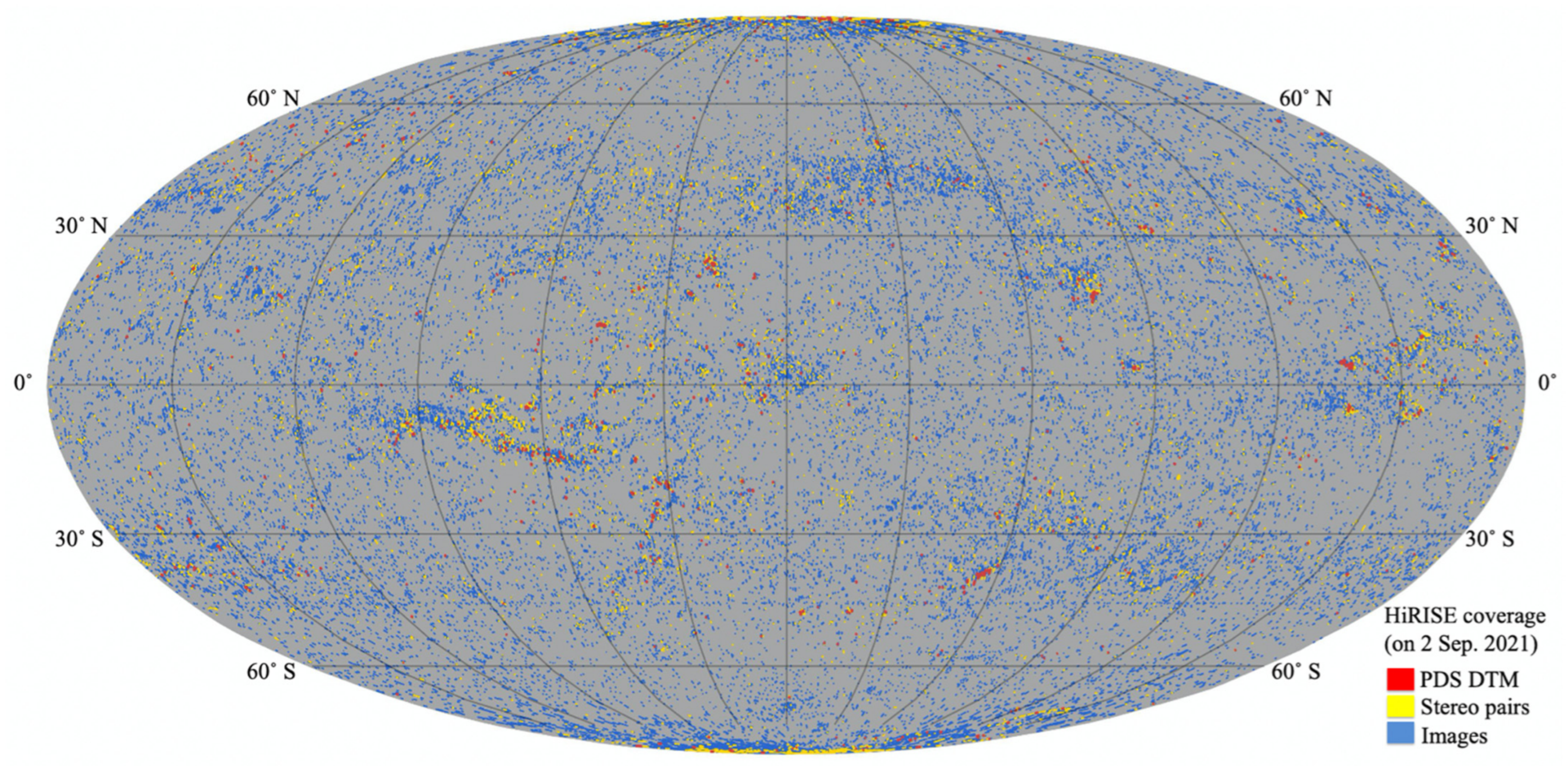
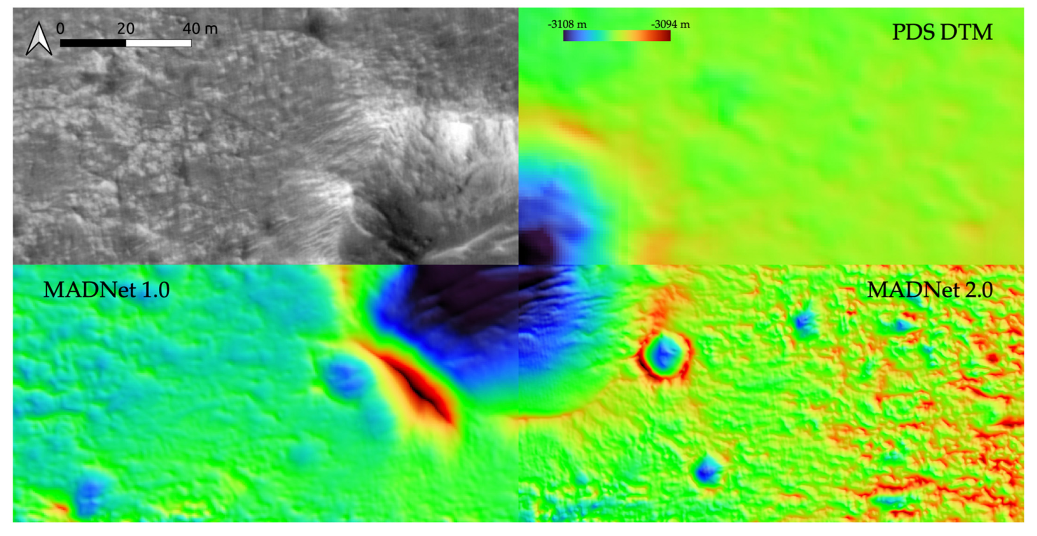
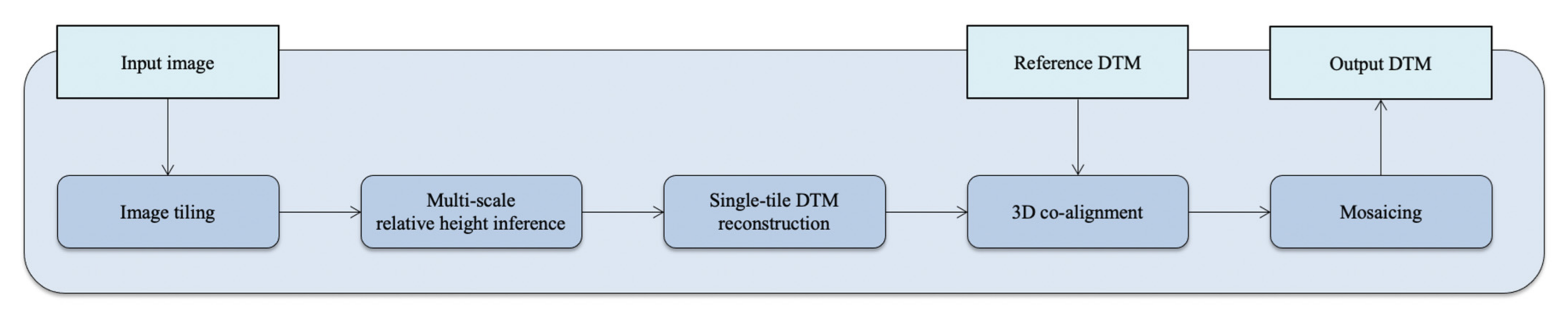
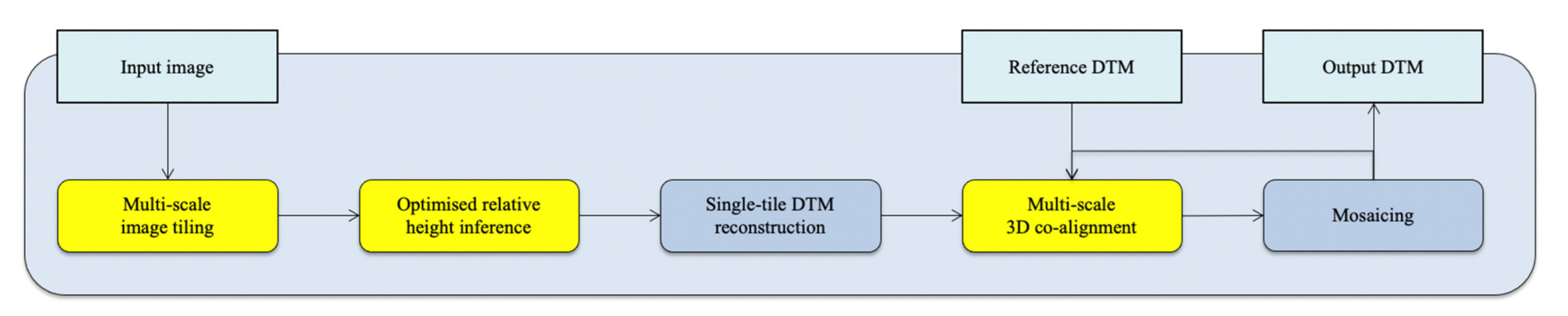
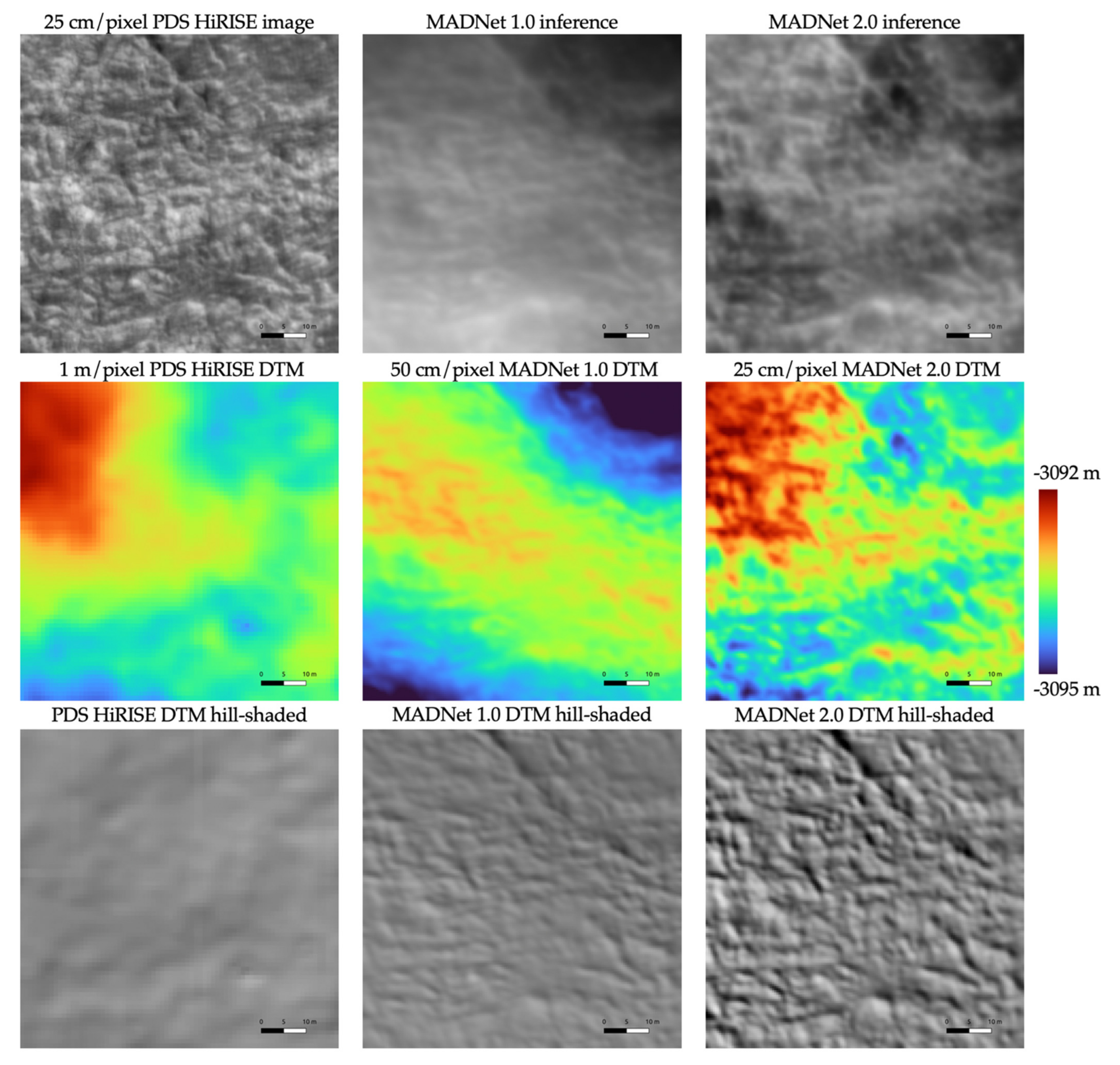
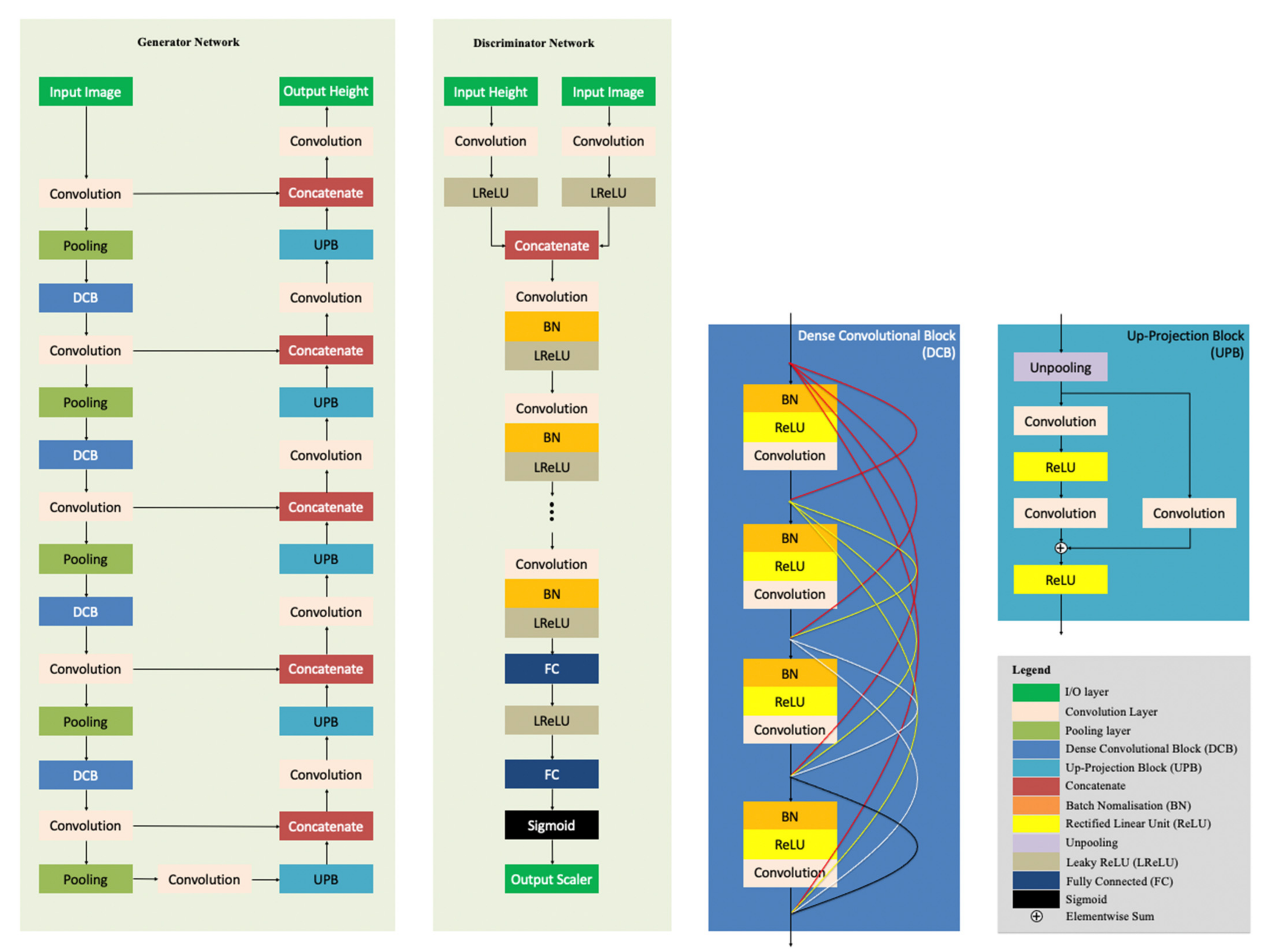
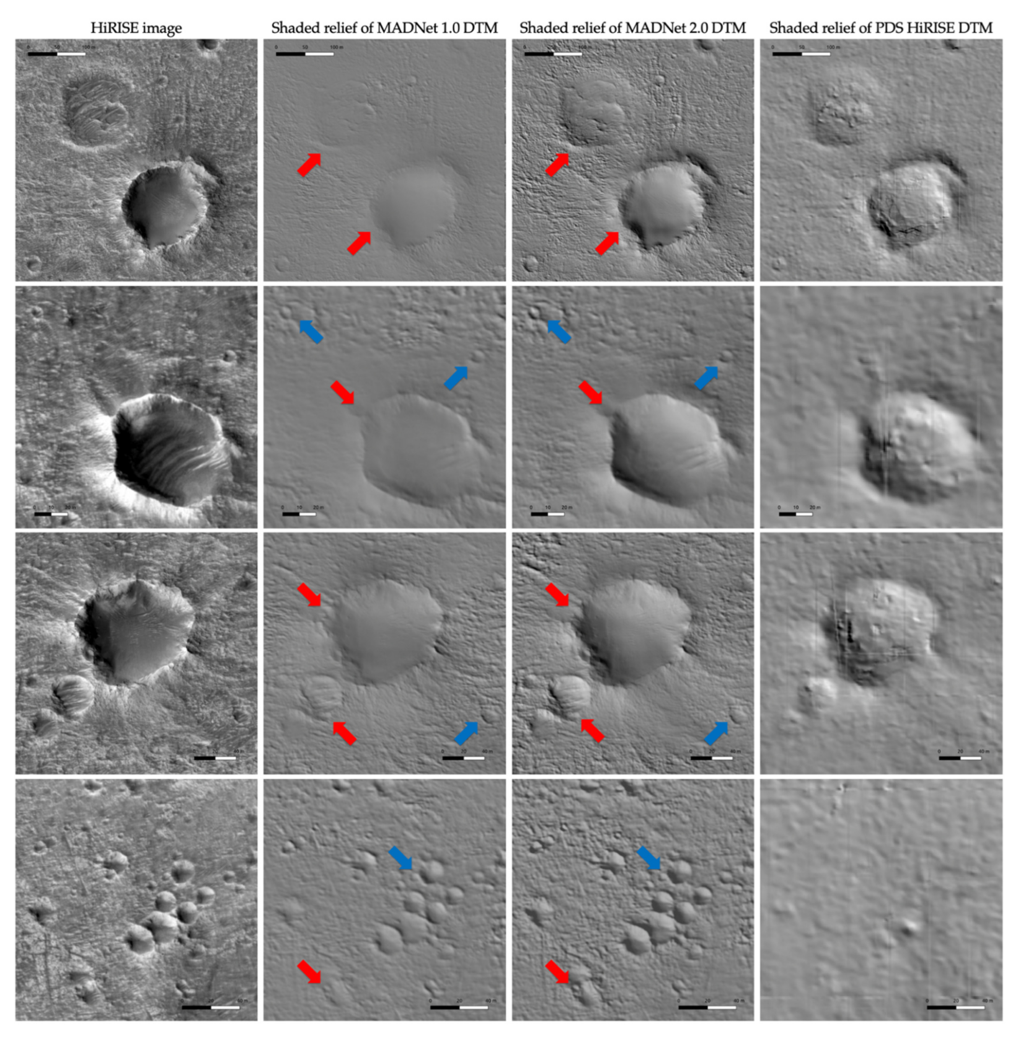
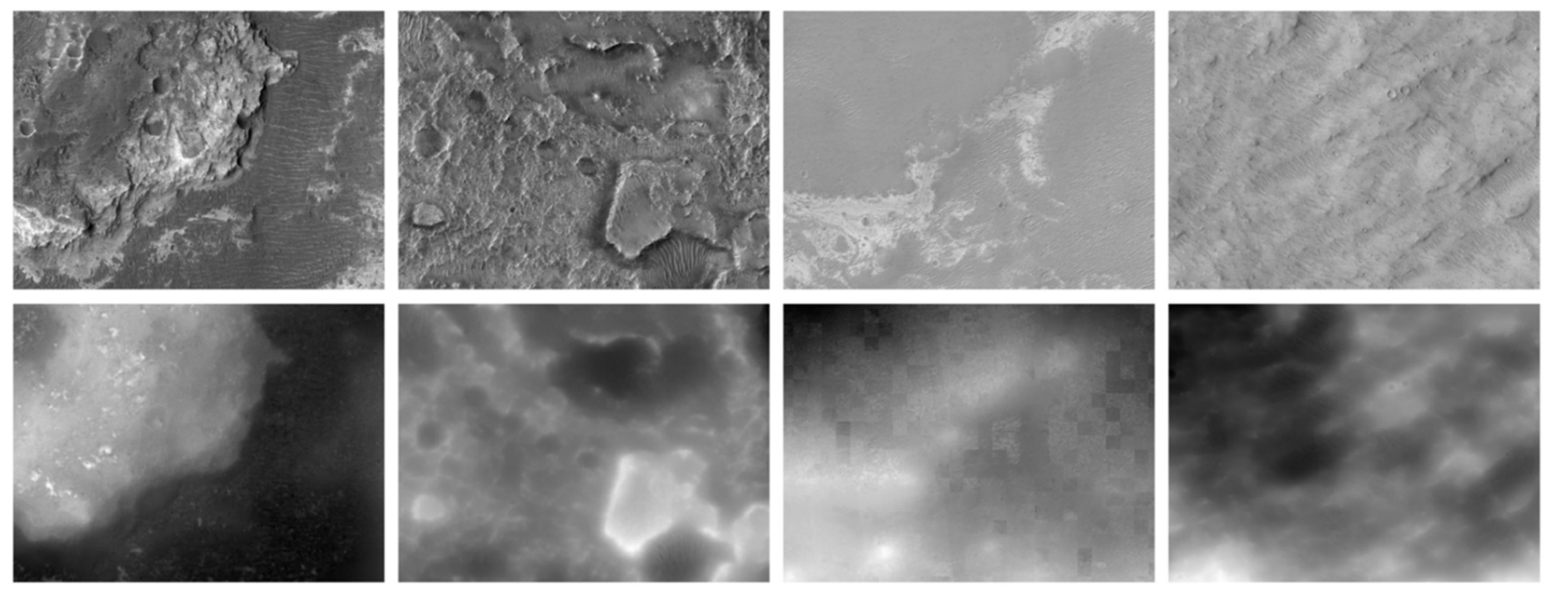
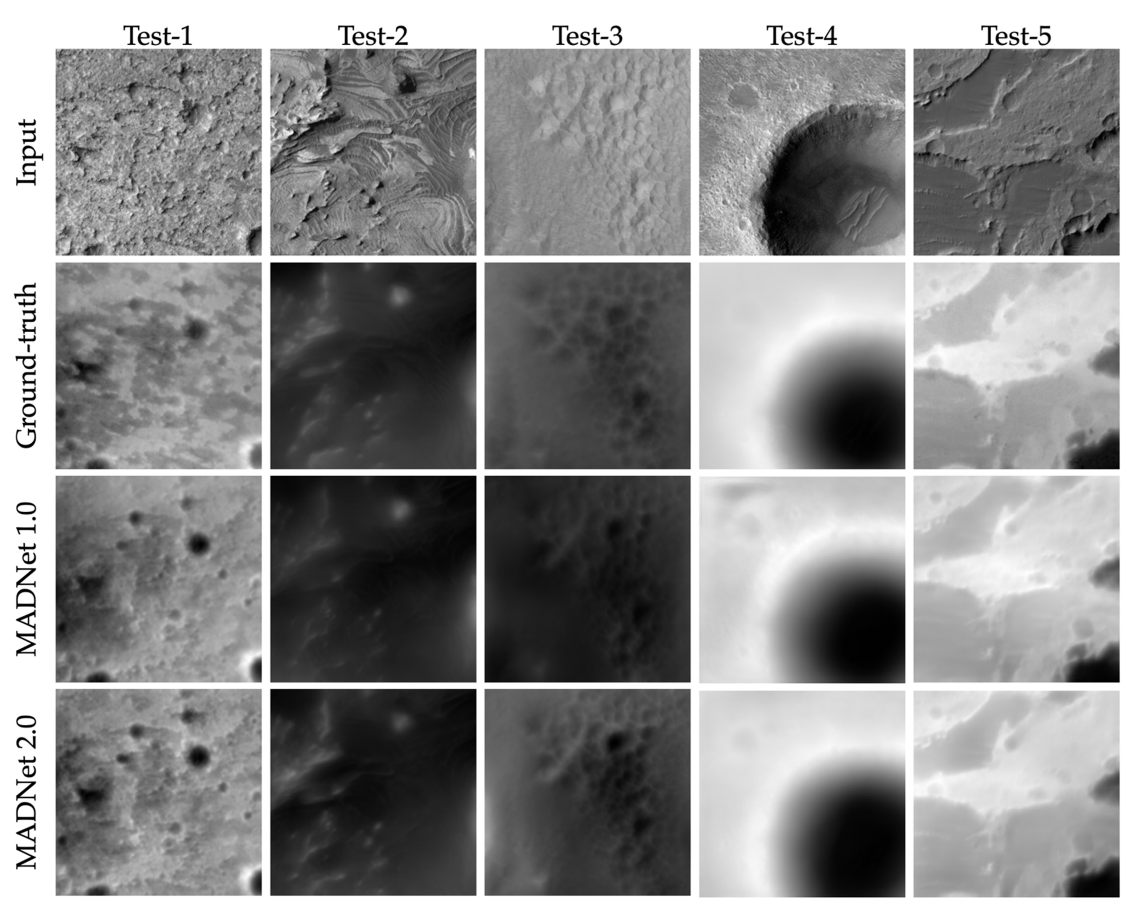
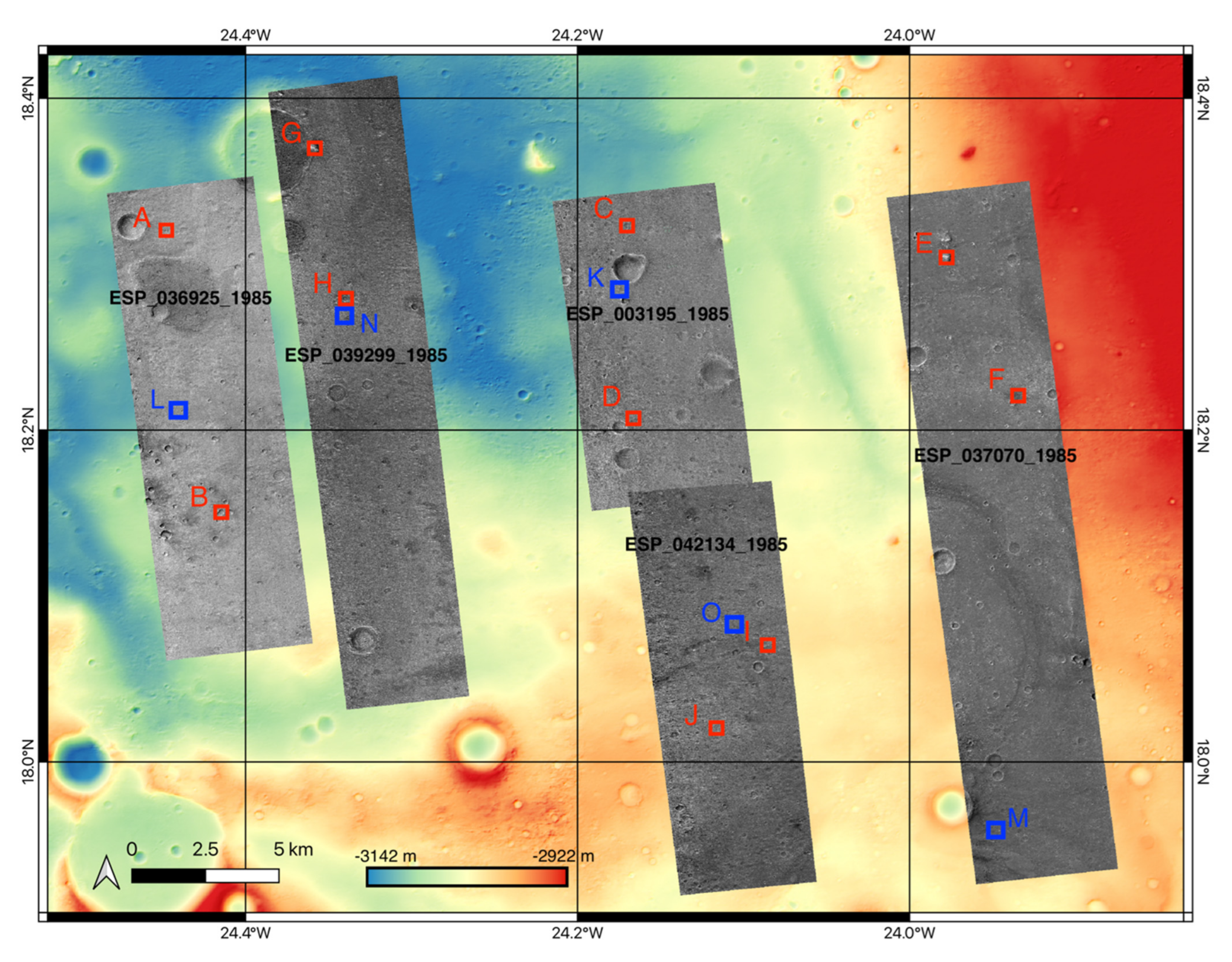
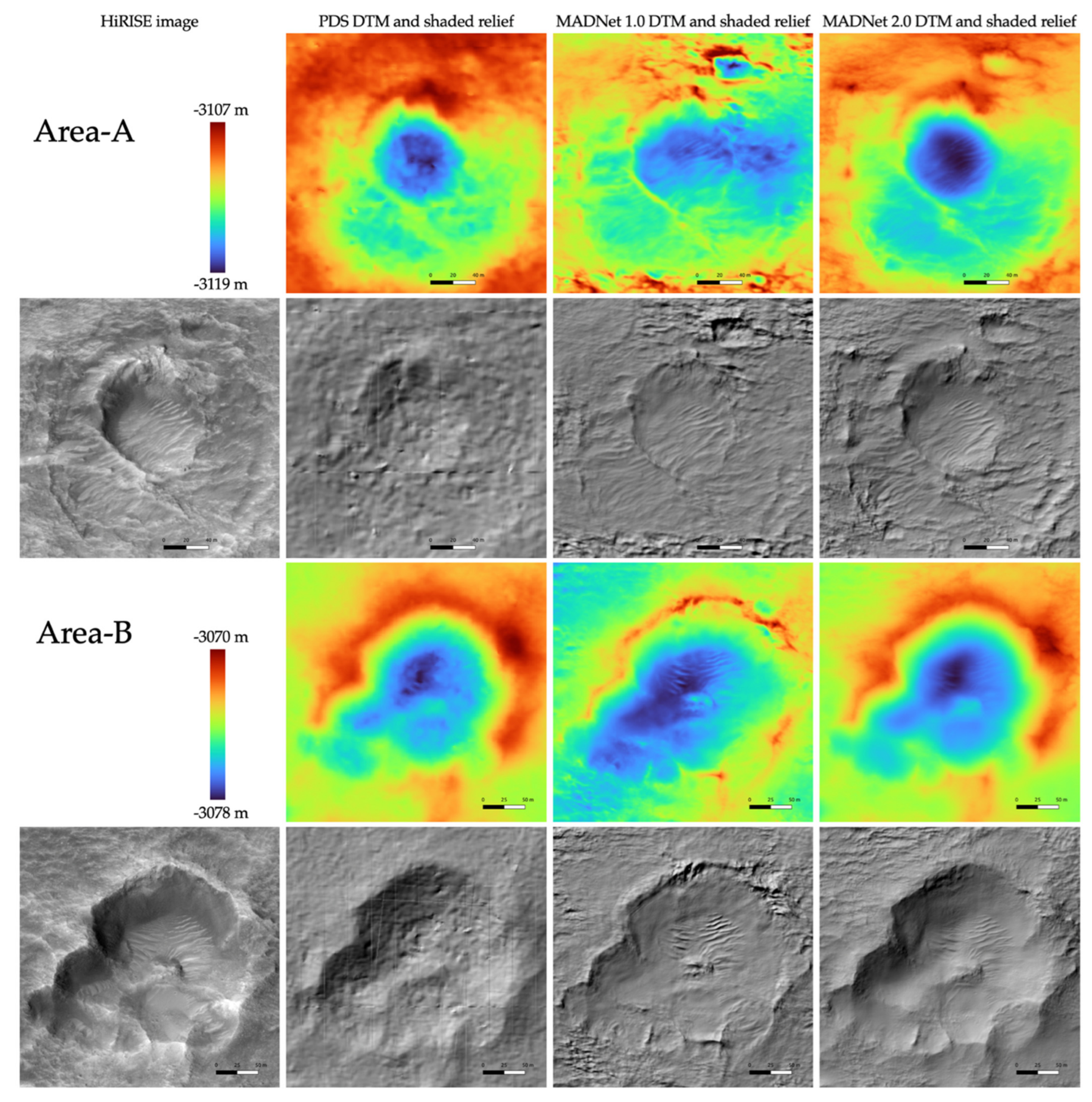
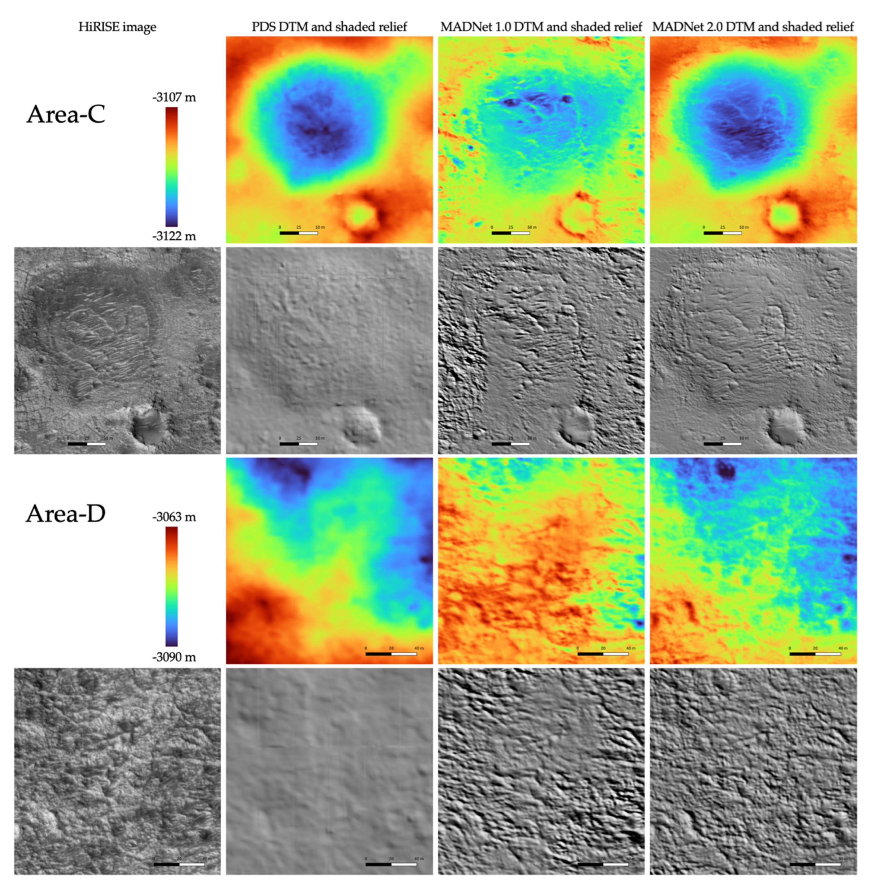
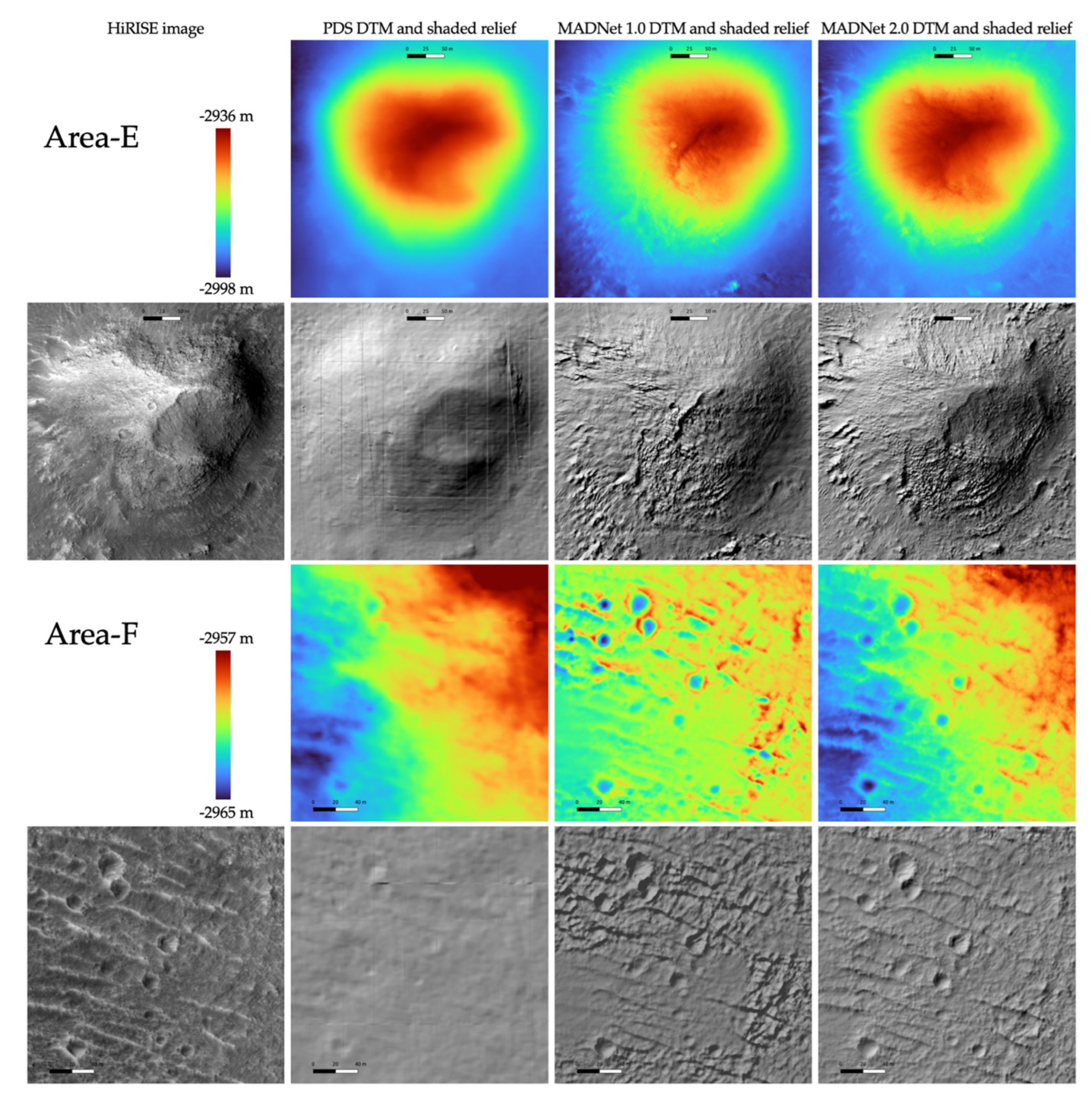
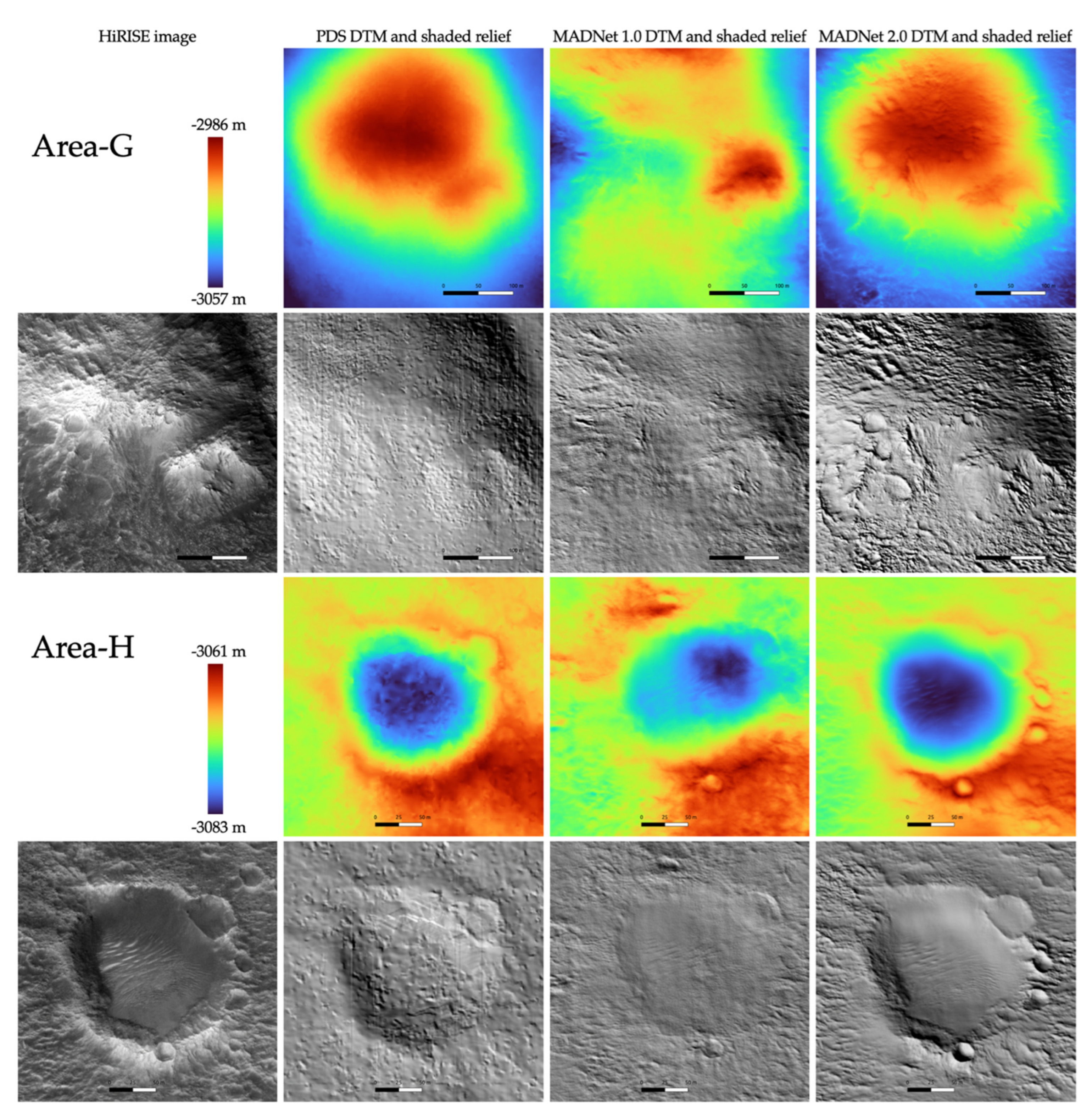
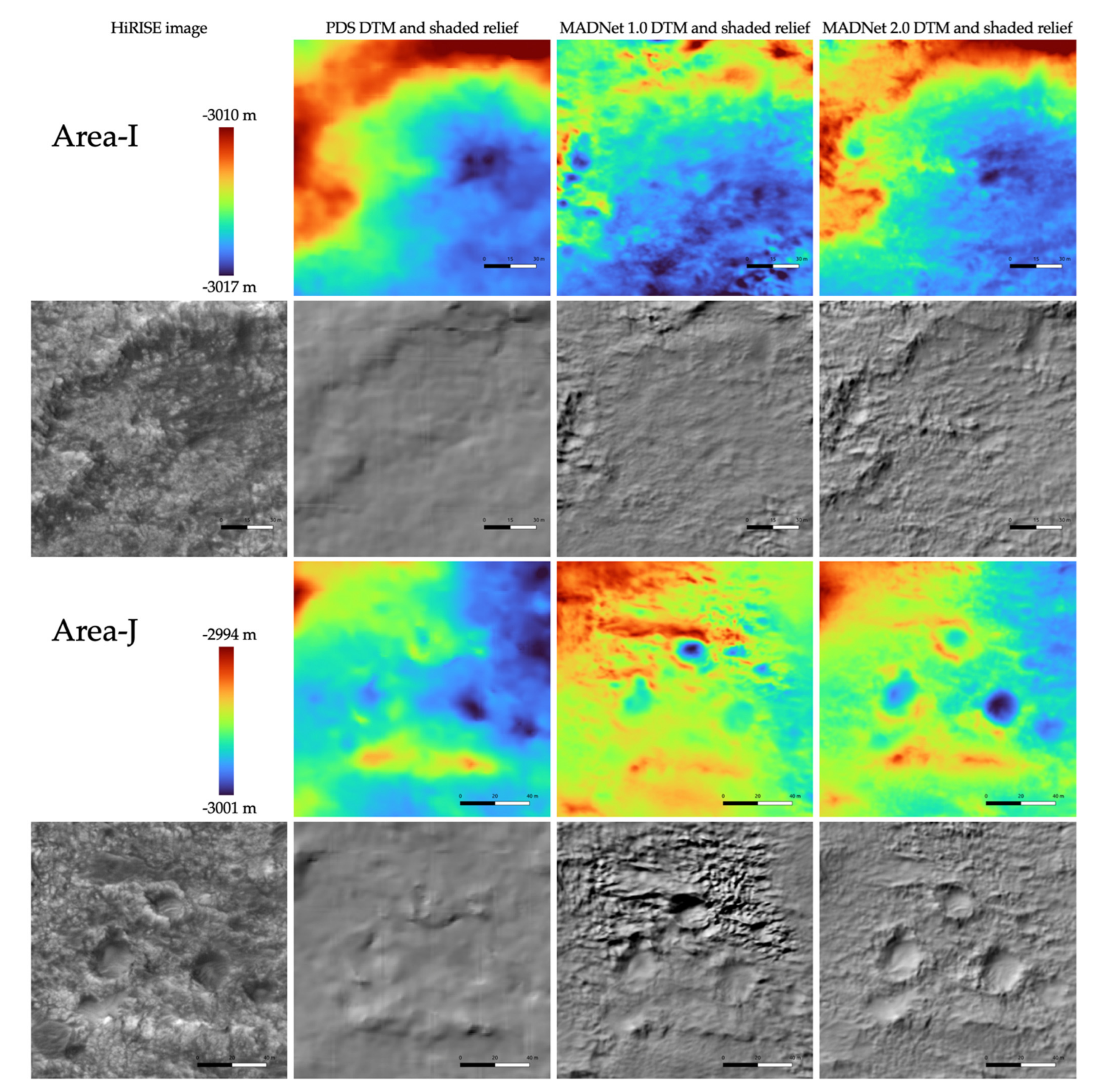
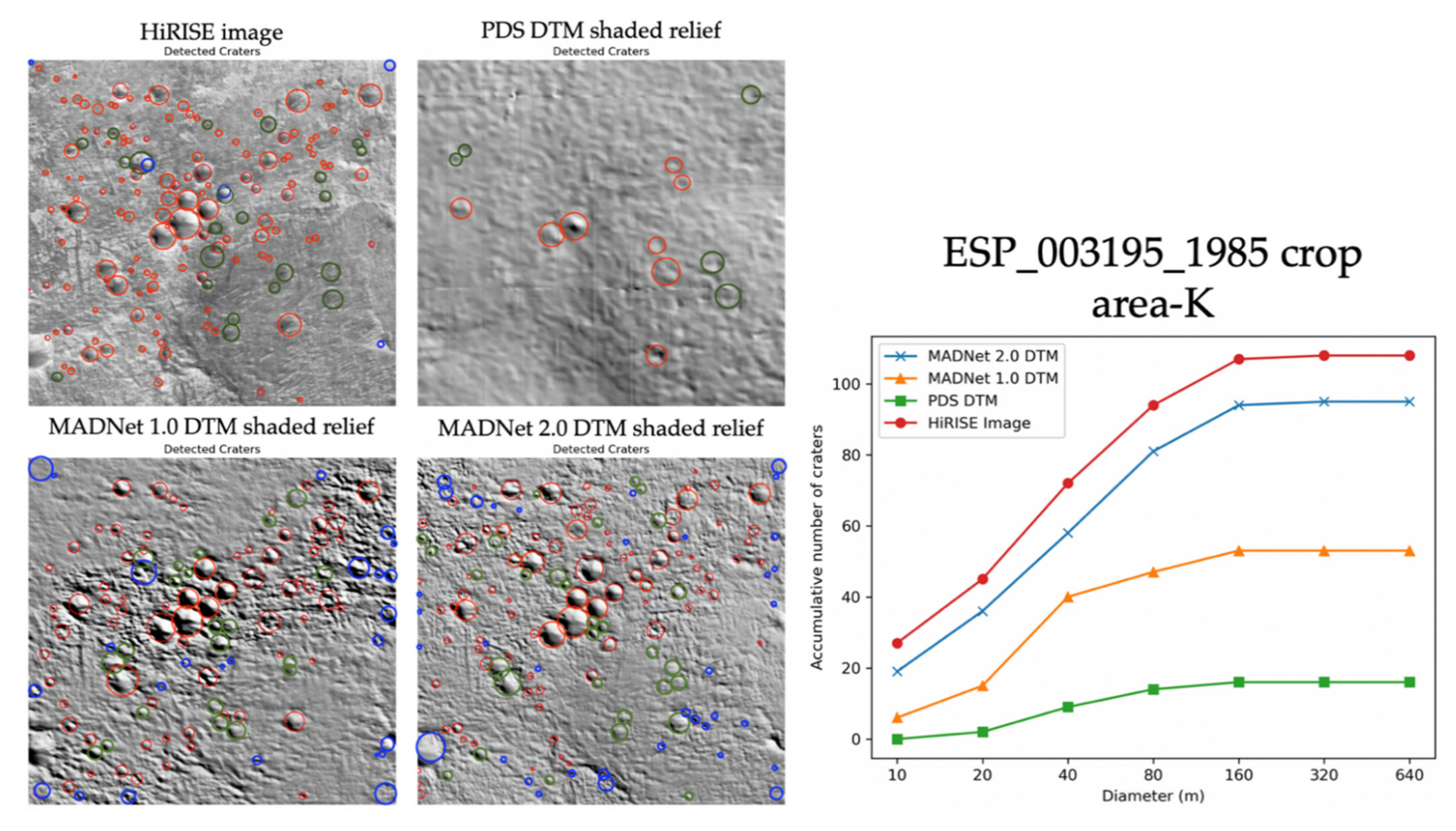
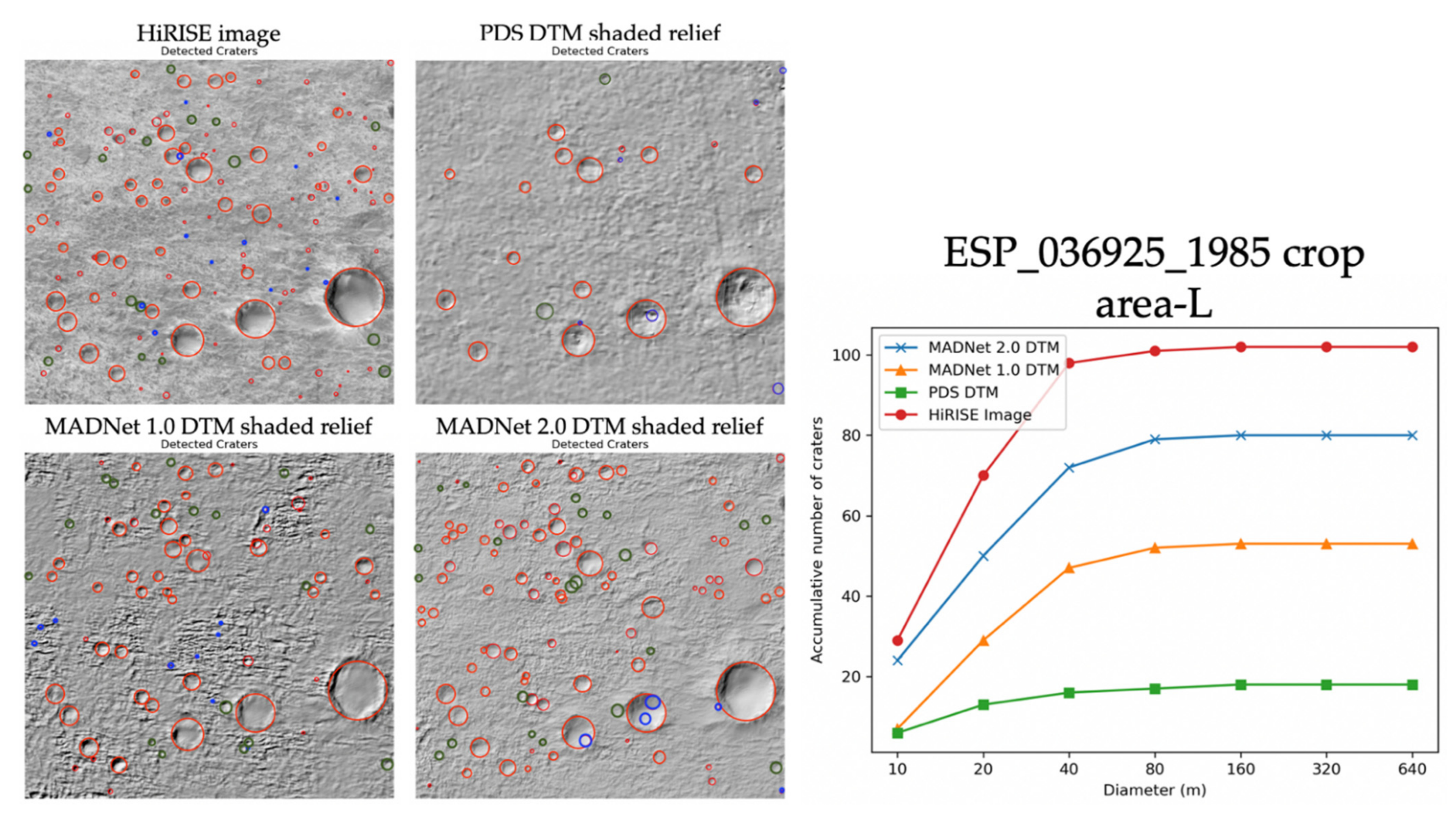
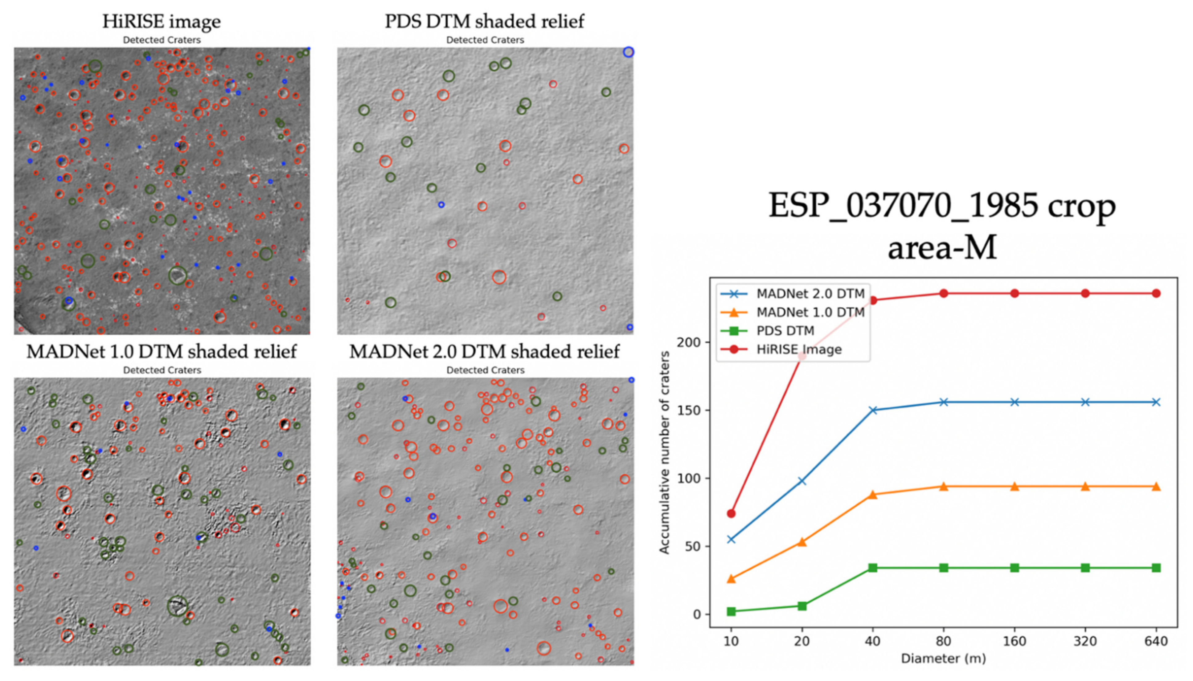
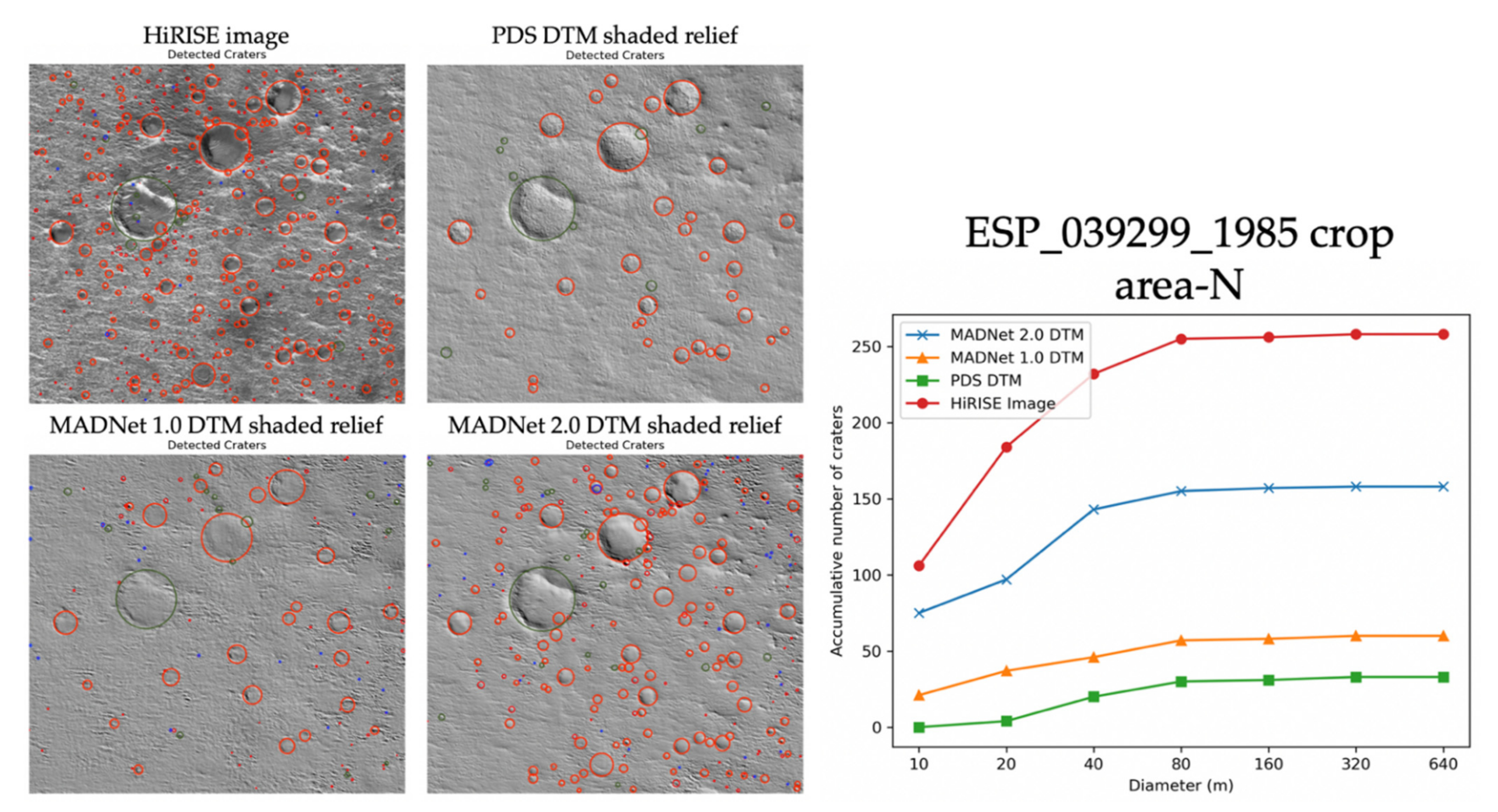
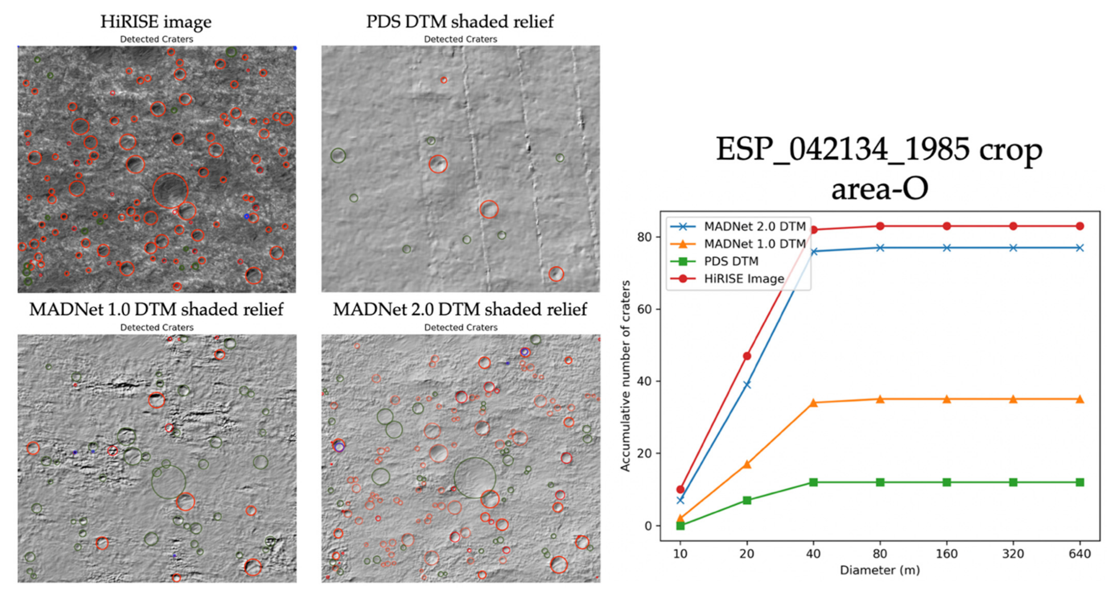
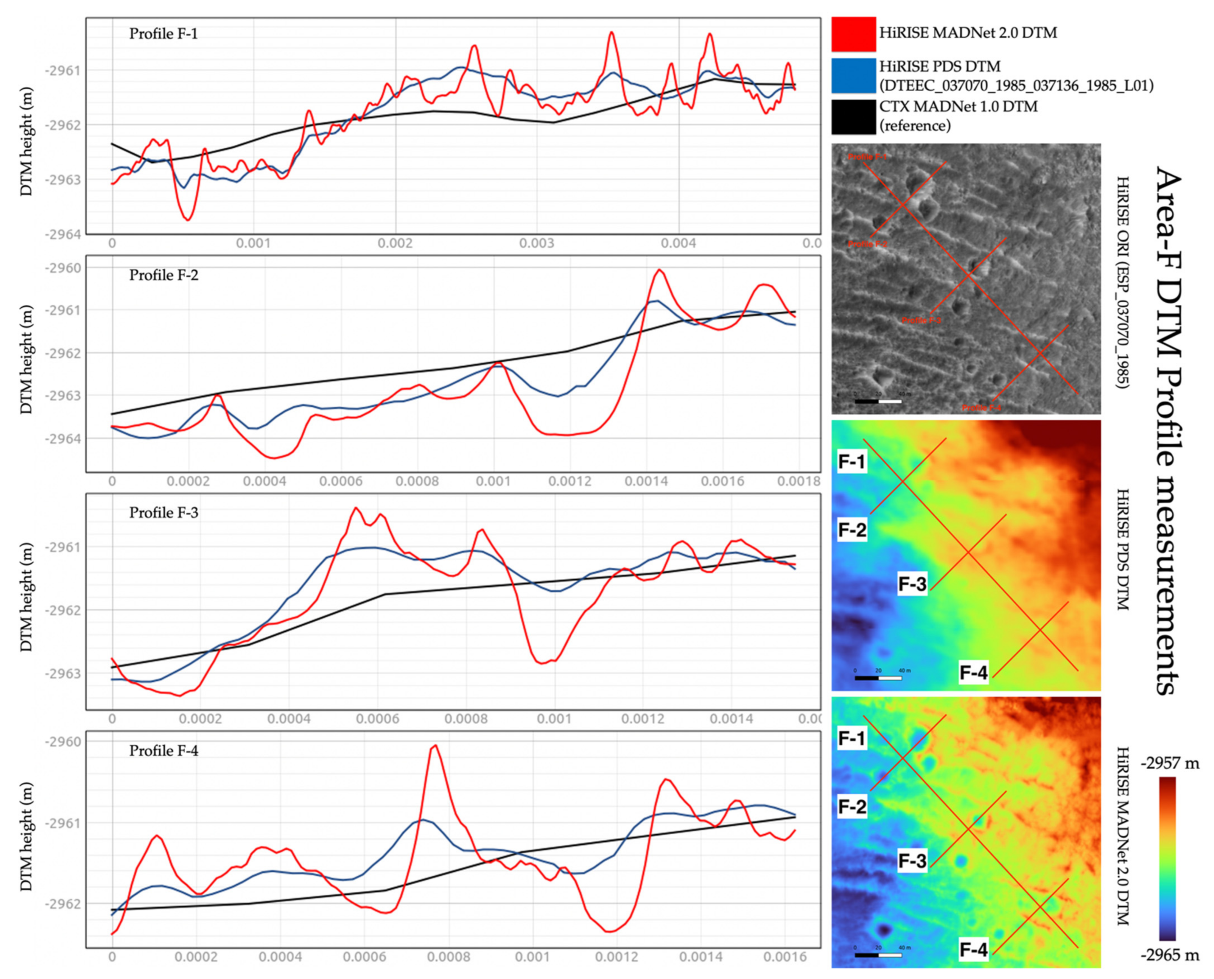
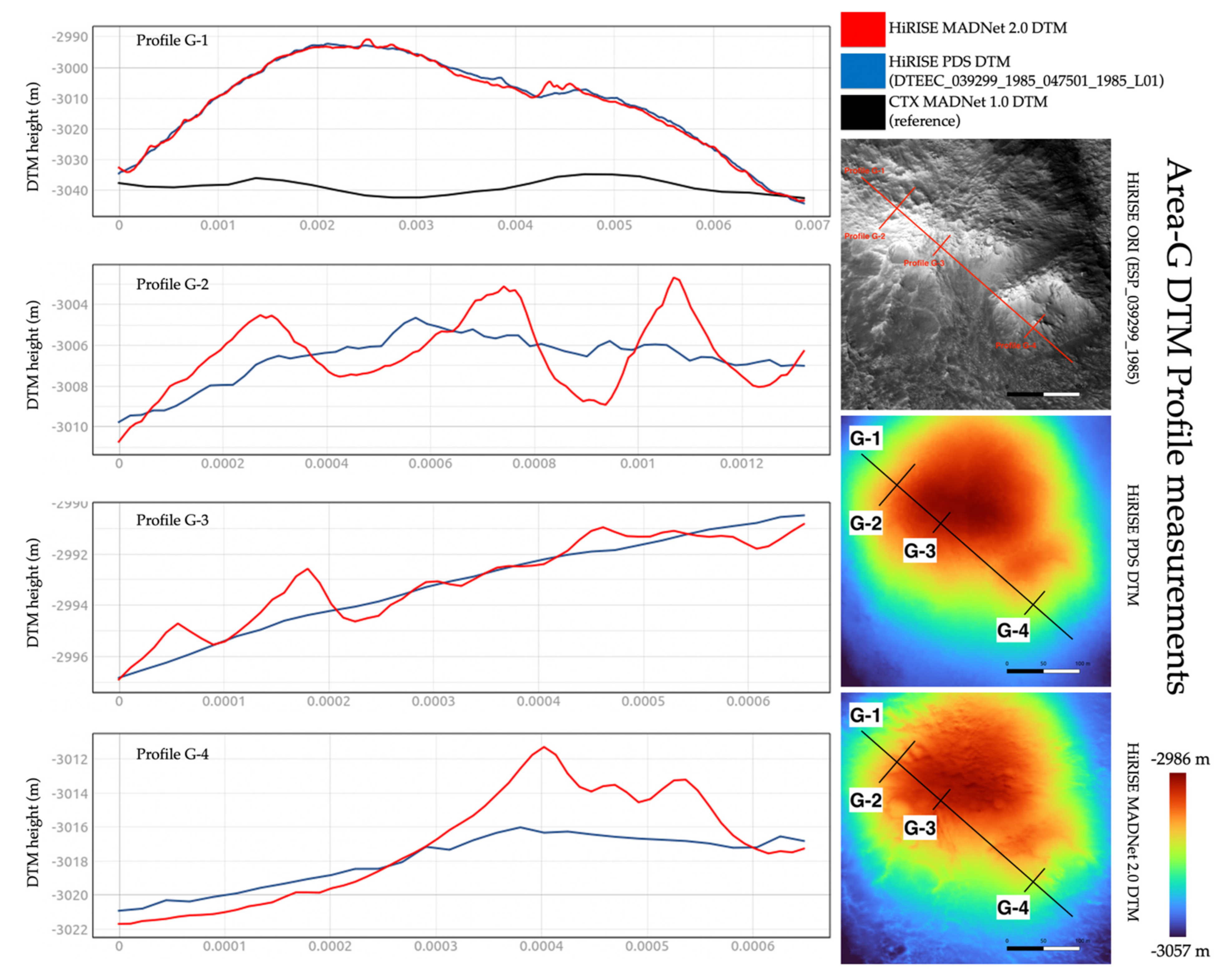
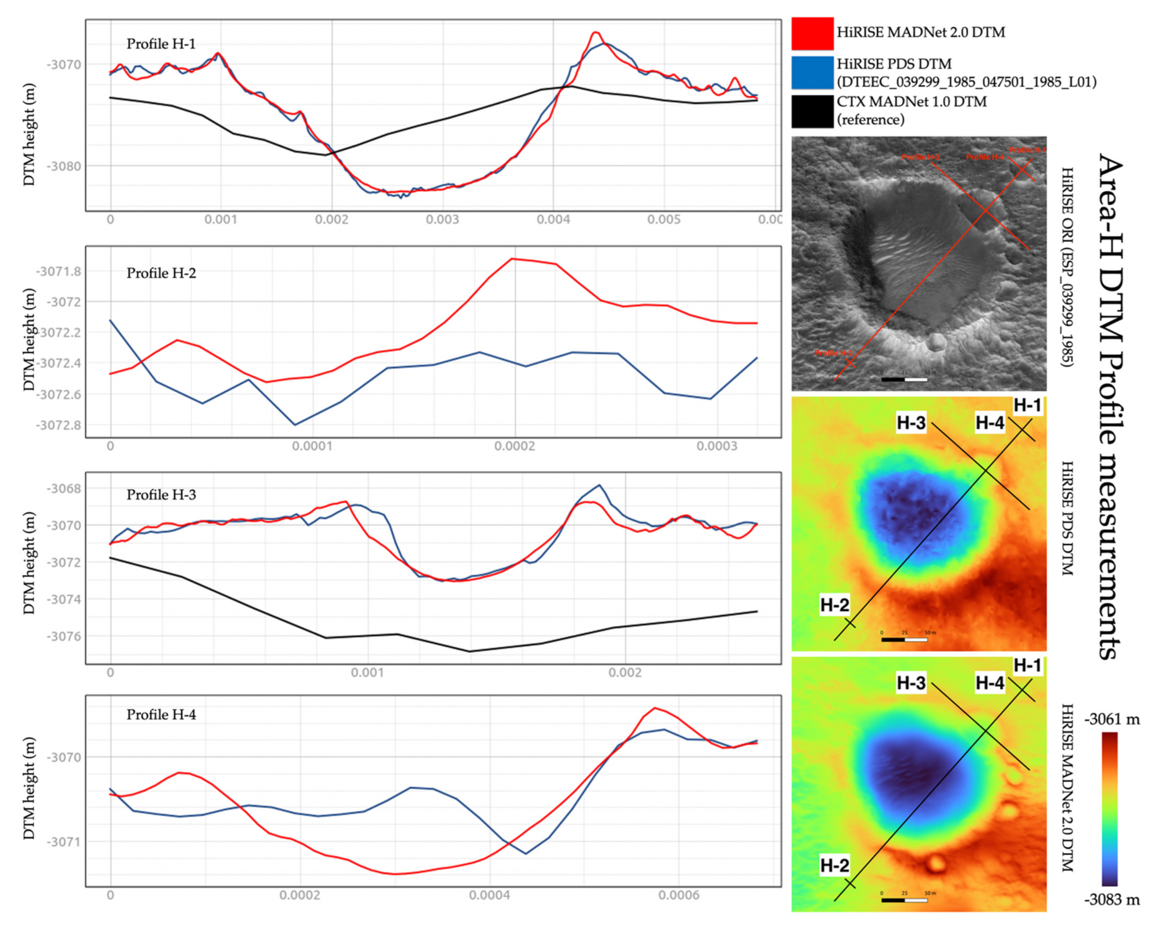
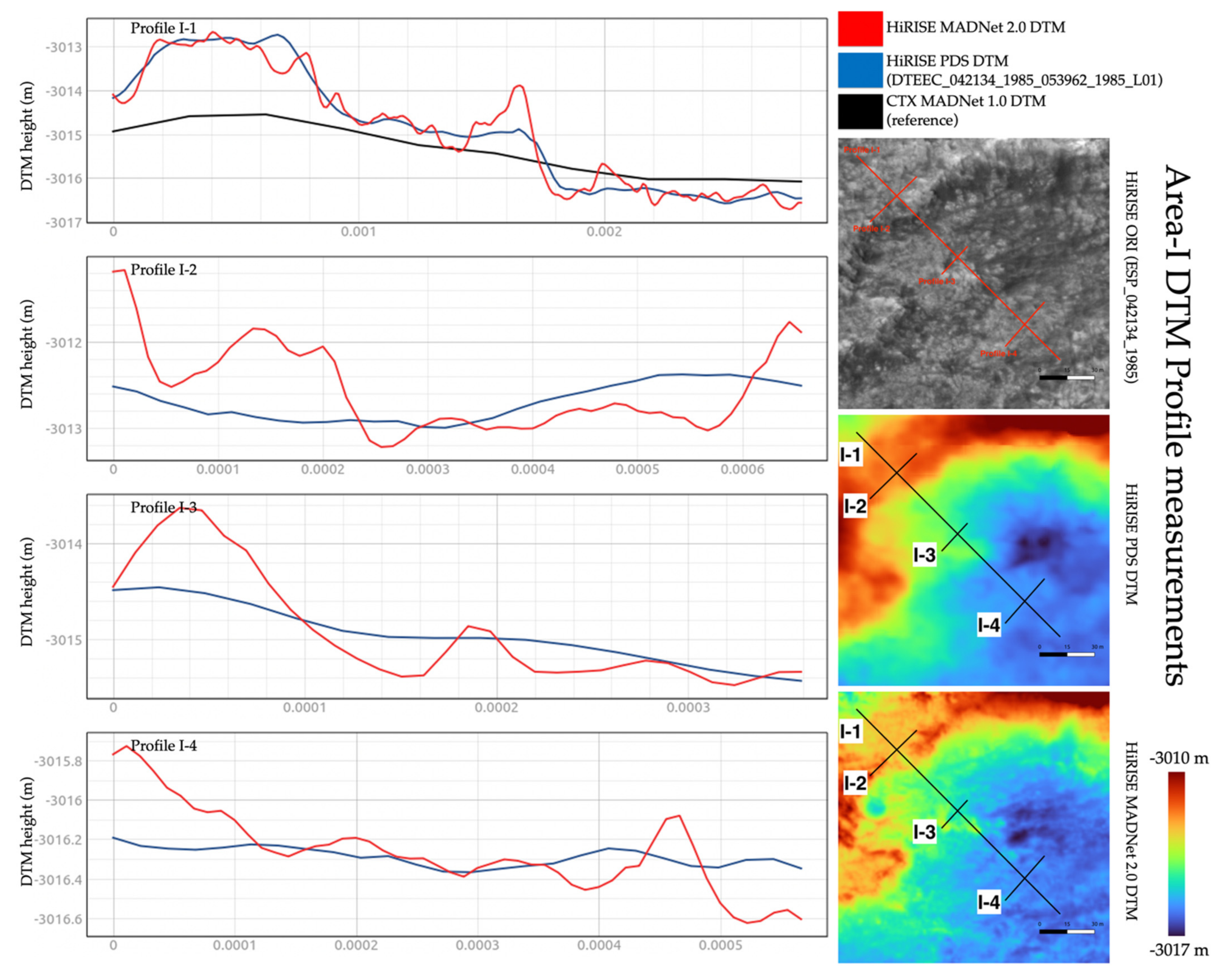
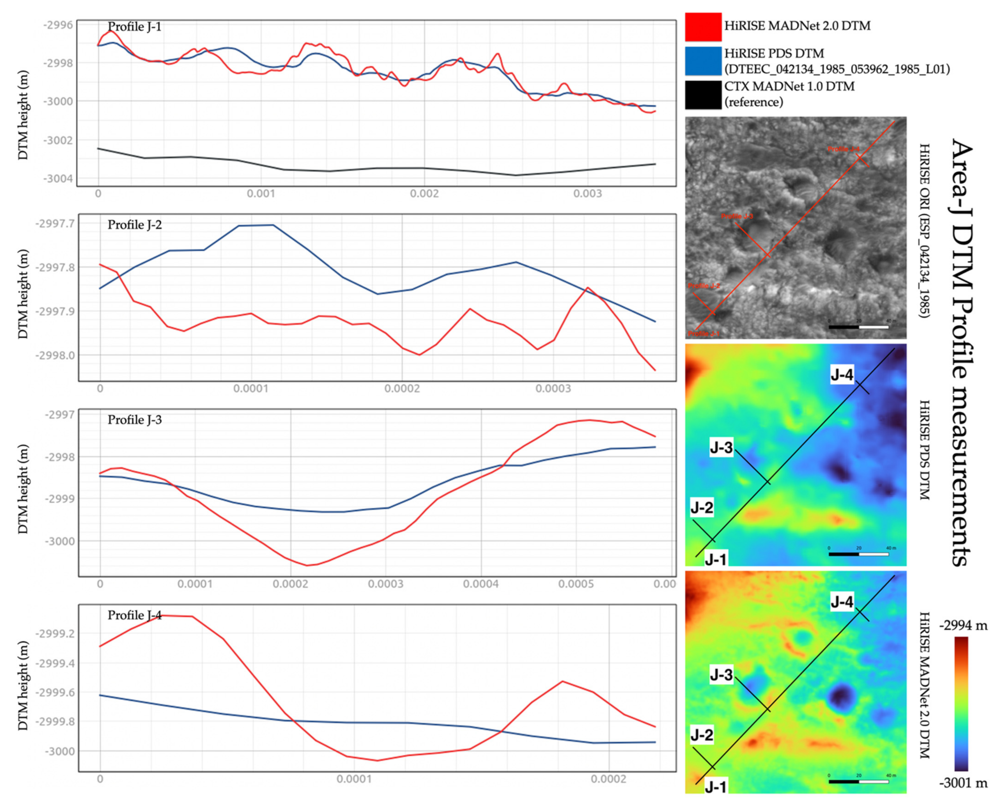
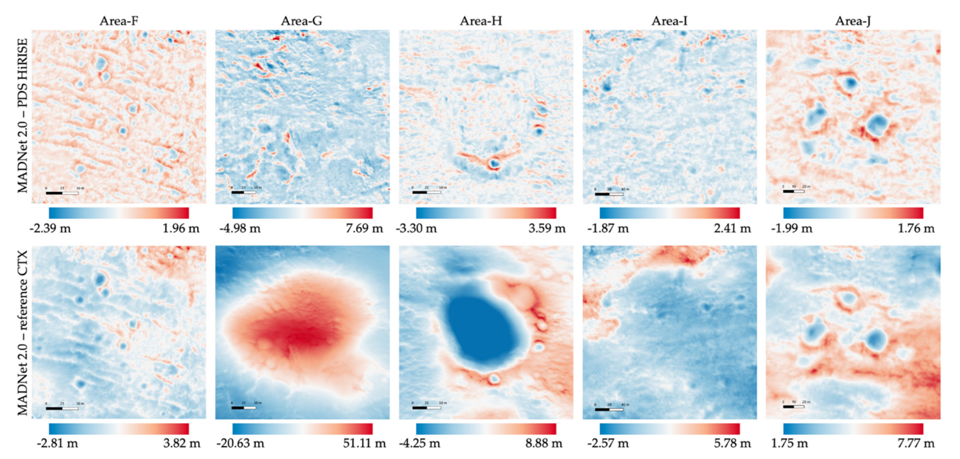
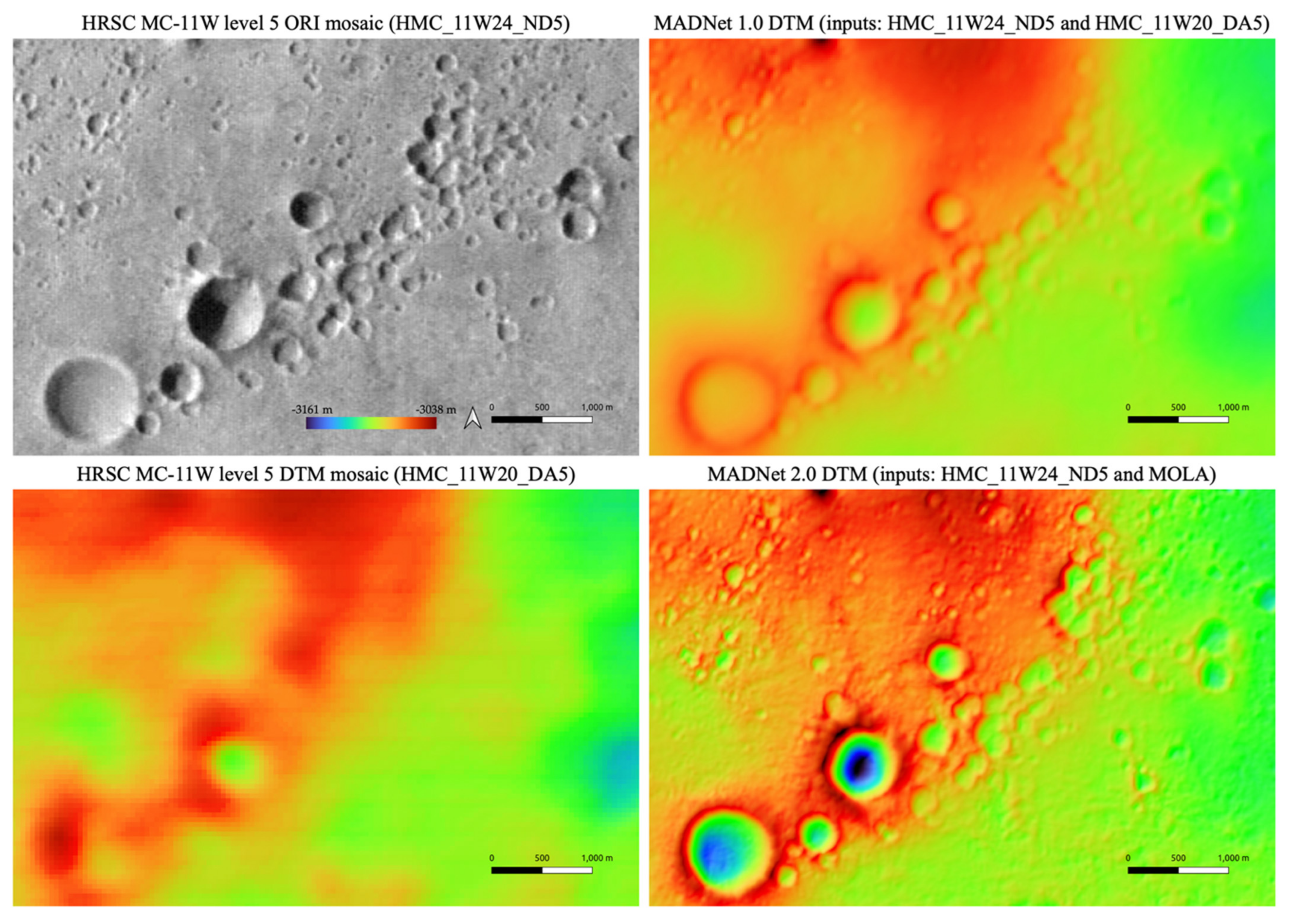
Table 1.
RMSEs and mean SSIMs of the MADNet 1.0 and MADNet 2.0 test results with respect to the PDS ground-truth for the five exemplar areas that are shown in Figure 9.
Table 1.
RMSEs and mean SSIMs of the MADNet 1.0 and MADNet 2.0 test results with respect to the PDS ground-truth for the five exemplar areas that are shown in Figure 9.
| Test-1 | Test-2 | Test-3 | Test-4 | Test-5 | ||
|---|---|---|---|---|---|---|
| MADNet 1.0 | RMSE (m) | 1.0892 | 0.8920 | 1.3501 | 1.2575 | 1.1727 |
| Mean SSIM | 0.9169 | 0.9308 | 0.7222 | 0.8702 | 0.7823 | |
| MADNet 2.0 | RMSE (m) | 0.9985 | 0.9286 | 1.1526 | 1.0999 | 1.1580 |
| Mean SSIM | 0.9235 | 0.9391 | 0.9253 | 0.8971 | 0.7851 | |
Table 2.
Summary of the ELF measurements of the HiRISE image, hill-shaded relief images of the MADNet 2.0 and MADNet 1.0 DTMs, for the four pre-selected areas for each of the five test HiRISE images.
Table 2.
Summary of the ELF measurements of the HiRISE image, hill-shaded relief images of the MADNet 2.0 and MADNet 1.0 DTMs, for the four pre-selected areas for each of the five test HiRISE images.
| HiRISE ID | Test-1 | Test-2 | Test-3 | Test-4 | Avg. M-FWHM in Pixels | |||||
|---|---|---|---|---|---|---|---|---|---|---|
| Extracted Edges | M-FWHM | Extracted Edges | M-FWHM | Extracted Edges | M-FWHM | Extracted Edges | M-FWHM | |||
| ESP_003195_1985 | HiRISE Image | - | 2.98 | - | 4.35 | - | 3.10 | - | 2.36 | 3.20 |
| MADNet 1.0 shaded relief | 83 | 3.26 | 37 | 6.05 | 301 | 4.90 | 89 | 4.57 | 4.45 | |
| MADNet 2.0 shaded relief | 83 | 3.01 | 58 | 4.85 | 301 | 3.98 | 89 | 2.41 | 3.56 | |
| ESP_036925_1985 | HiRISE Image | - | 2.92 | - | 2.90 | - | 2.70 | - | 3.32 | 2.96 |
| MADNet 1.0 shaded relief | 117 | 3.46 | 395 | 4.17 | 162 | 3.79 | 216 | 4.22 | 3.91 | |
| MADNet 2.0 shaded relief | 117 | 3.22 | 395 | 3.01 | 162 | 2.92 | 216 | 3.35 | 3.13 | |
| ESP_037070_1985 | HiRISE Image | - | 3.74 | - | 3.67 | - | 3.13 | - | 3.91 | 3.61 |
| MADNet 1.0 shaded relief | 92 | 3.94 | 13 | 4.32 | 277 | 5.07 | 21 | 4.84 | 4.54 | |
| MADNet 2.0 shaded relief | 92 | 4.03 | 17 | 4.77 | 277 | 3.16 | 25 | 4.53 | 4.12 | |
| ESP_039299_1985 | HiRISE Image | - | 3.58 | - | 2.76 | - | 3.16 | - | 2.95 | 3.11 |
| MADNet 1.0 shaded relief | 122 | 6.48 | 22 | 4.70 | 80 | 5.95 | 52 | 3.58 | 5.18 | |
| MADNet 2.0 shaded relief | 122 | 6.21 | 22 | 2.84 | 84 | 6.12 | 54 | 3.46 | 4.66 | |
| ESP_042134_1985 | HiRISE Image | - | 2.94 | - | 2.83 | - | 3.38 | - | 3.10 | 3.06 |
| MADNet 1.0 shaded relief | 64 | 6.77 | 248 | 3.16 | 169 | 5.52 | 20 | 3.40 | 4.71 | |
| MADNet 2.0 shaded relief | 65 | 3.25 | 248 | 3.08 | 172 | 5.69 | 49 | 3.33 | 3.84 | |
Table 3.
Statistics (mean and standard deviations) of the DTM difference maps that are shown in Figure 26.
Table 3.
Statistics (mean and standard deviations) of the DTM difference maps that are shown in Figure 26.
| Area-F | Area-G | Area-H | Area-I | Area-J | ||
|---|---|---|---|---|---|---|
| MADNet 2.0 HiRISE DTM - PDS HiRISE DTM | Mean | 0.001 m | −0.013 m | −0.20 m | −0.005 m | −0.003 m |
| Standard Deviation | 0.289 m | 1.073 m | 0.435 m | 0.297 m | 0.304 m | |
| MADNet 2.0 HiRISE DTM - CTX reference DTM | Mean | 0.076 m | 6.059 m | 1.155 m | 0.292 m | 4.868 m |
| Standard Deviation | 0.601 m | 16.381 m | 2.804 m | 1.218 m | 0.886 m | |
Publisher’s Note: MDPI stays neutral with regard to jurisdictional claims in published maps and institutional affiliations. |
© 2021 by the authors. Licensee MDPI, Basel, Switzerland. This article is an open access article distributed under the terms and conditions of the Creative Commons Attribution (CC BY) license (https://creativecommons.org/licenses/by/4.0/).
Share and Cite
MDPI and ACS Style
Tao, Y.; Muller, J.-P.; Xiong, S.; Conway, S.J. MADNet 2.0: Pixel-Scale Topography Retrieval from Single-View Orbital Imagery of Mars Using Deep Learning. Remote Sens. 2021, 13, 4220. https://0-doi-org.brum.beds.ac.uk/10.3390/rs13214220
AMA Style
Tao Y, Muller J-P, Xiong S, Conway SJ. MADNet 2.0: Pixel-Scale Topography Retrieval from Single-View Orbital Imagery of Mars Using Deep Learning. Remote Sensing. 2021; 13(21):4220. https://0-doi-org.brum.beds.ac.uk/10.3390/rs13214220
Chicago/Turabian StyleTao, Yu, Jan-Peter Muller, Siting Xiong, and Susan J. Conway. 2021. "MADNet 2.0: Pixel-Scale Topography Retrieval from Single-View Orbital Imagery of Mars Using Deep Learning" Remote Sensing 13, no. 21: 4220. https://0-doi-org.brum.beds.ac.uk/10.3390/rs13214220
Note that from the first issue of 2016, this journal uses article numbers instead of page numbers. See further details here.