1. Introduction
Precipitating hydrometeors undergo various processes as they fall, including water vapour condensation, coalescence, break-up or evaporation for liquid water and ice nucleation, riming, aggregation or accretion for the solid phase [
1]. One of the most important processes occurs as falling particles cross the 0 °C isotherm level, also called melting level, where solid water particles begin to melt and eventually transform completely into liquid particles [
2,
3]. The atmospheric layer where this process takes place is known as the melting layer and may produce a characteristic radar signature, the so-called radar Bright Band (hereafter BB), a term originated from the local maxima caused by high reflectivity values visible in the equivalent reflectivity vertical profile [
4]. The BB is caused by differences in the dielectric constants, shape and terminal fall speeds of liquid and solid hydrometeor precipitating particles, which lead to abrupt changes of the radar backscattered power within the BB. The most evident BB signatures are produced under stratiform cold rain conditions [
5,
6] as updrafts, and vertical mixing present in convective precipitation do not provide the proper conditions for BB formation.
The presence of a BB in volumetric operational weather radar observations may produce local overestimations of rainfall amounts, which has led to the development of different procedures to detect and correct BB effects [
2,
7,
8,
9]. This is particularly important for events with rapidly changing characteristics, for example, with quick transitions from snow to rain [
10,
11,
12], or in the development of subsequent robust applications of radar precipitation estimates, such as hydrological modelling or NWP assimilation [
13,
14,
15].
Most of the above BB correction schemes for scanning weather radars are based on more specific studies, typically performed with vertically pointing radars or using the so-called quasi vertical profiles of polarimetric scanning weather radars [
16], not only to detect but also to characterise, in detail, the BB. The methods proposed include the use of the signal to noise ratio (SNR), the Doppler velocity profile [
3], vertical gradients of equivalent radar reflectivity or Doppler velocity [
17,
18,
19,
20,
21], or different polarimetric variables if polarimetric radars are used [
16,
22,
23]. Other studies examined the relationship between the 0 °C dry-bulb temperature isotherm level and the BB height [
24], which requires additional data, i.e., the temperature profile, typically obtained from radiosonde observations. Recent research related to BB effects has examined cases with multiple melting ice particle layers [
22], the relation of BB intensity to surface rainfall rate [
25] or BB effects upon spaceborne radar observations [
26,
27].
The main objective of this article is to describe a new processing methodology to detect the BB with single polarisation vertically pointing Doppler radar spectral observations, based on the use of the third moment of the Doppler radar velocity spectrum, the skewness. The new detection algorithm is implemented for a compact frequency-modulated continuous-wave (FMCW) vertically pointing Doppler radar operating in the K-band. The radar model used here is an MRR-Pro, which also provides a processing software that, among other variables, computes the existence of a melting layer (ML) given by a probability value (from 0 to 1). The methodology proposed here also provides an alternative signal processing with an advanced new dealiasing scheme in order to deal with some cases where the original manufacturer software provides limited results. The equivalent reflectivity provided by the new signal and noise detection scheme is compared with co-located Parsivel observations. The proposed BB detection scheme is compared with the MRR manufacturer ML product and also with co-located radiosounding observations.
The paper is organised as follows. In
Section 2, we detail the instrumentation used.
Section 3 describes the methodology and the improvements performed to avoid the aliasing and the new technique to determine the BB. We show the results in
Section 4, a discussion in
Section 5 and in
Section 6, we present the conclusions.
2. Instrumentation and Data Acquisition
2.1. Instrumentation
The main instrument used in this study was a K-band (24 GHz) Doppler radar, MRR (Micro Rain Radar) manufactured by Metek Gmbh, model MRR-
Pro, located on the roof of the Faculty of Physics building of the University of Barcelona (41°23′4.34″ N, 2°7′3.05″ E). MRR-
Pro is an updated version of previous MRR units [
28]. The configuration parameters used in the study (
Table 1) provided precipitation observations up to 6.4 km above the radar level with a vertical resolution of 50 m and a temporal resolution of 10 s.
An OTT Parsivel-2 disdrometer [
29], hereafter Parsivel, co-located with the MRR-
Pro, provided precipitation particle size and fall speed spectra at the radar level. These parameters allow comparisons between the MRR-
Pro and Parsivel for different variables, such as rainfall rate or radar reflectivity. Finally, on the same roof is located the Barcelona radio sounding station (WMO code 08190), which performs two soundings a day (at 00 and 12 UTC) that were also used in this study.
2.2. Data Acquisition
The data files generated by the MRR-
Pro manufacturer software are used as input files for the processing with RaProM-
Pro. These files are in netcdf format and contain basic configuration settings of the data acquisition, the raw data (so-called spectral reflectivity, or spectrum raw according to the manufacturer) and derived parameters, such as radial velocity spectra or an estimate of existence of the melting layer.
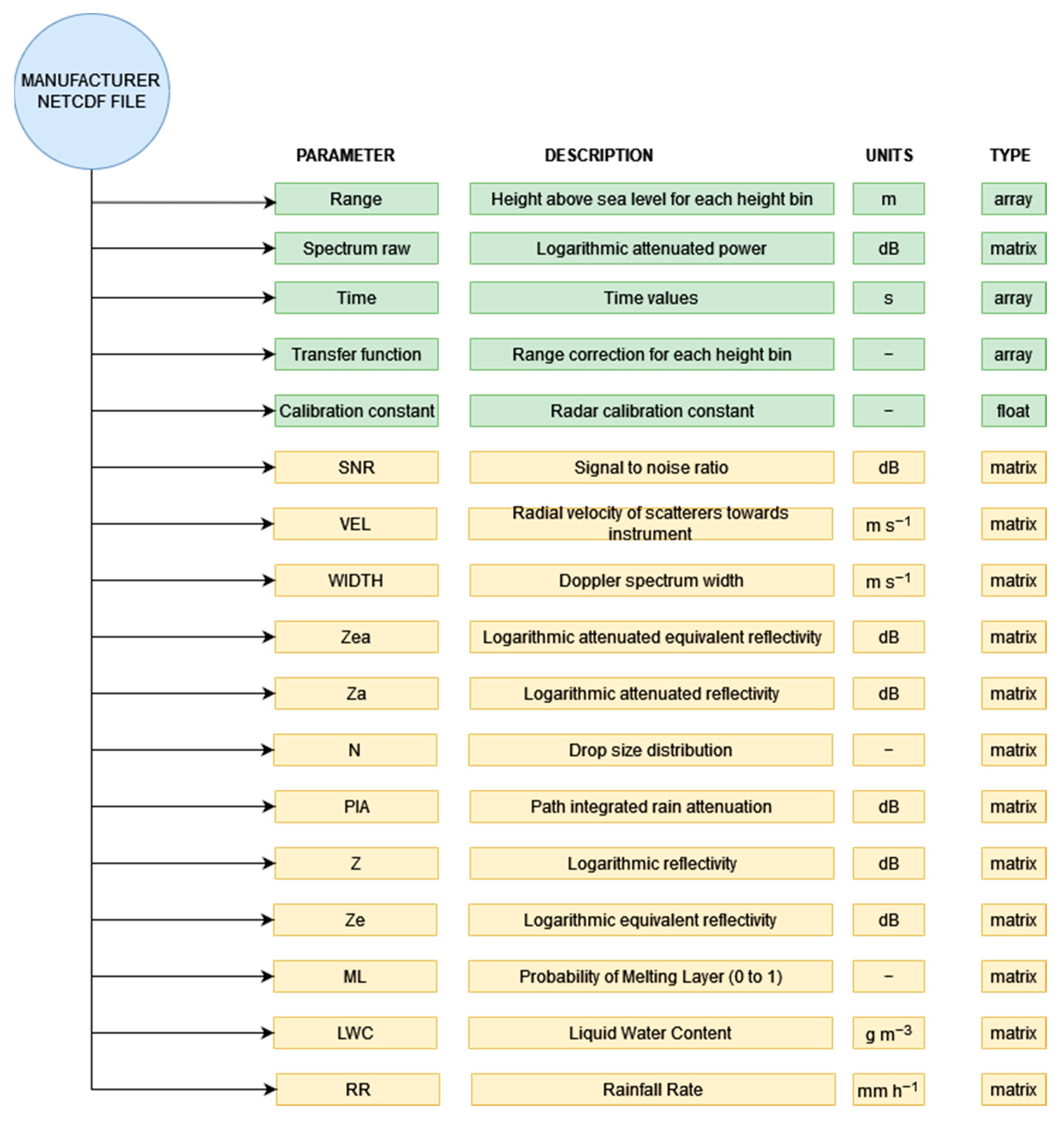
Figure 1 schematically shows a selection of the content of the files and also indicates which variables are used in the proposed methodology (shown in green), which are, essentially, configuration parameters and raw data, from which derived parameters can be calculated.
The parameters used by RaProM-Pro include, for each time step, a matrix s(n, i) with the spectral raw values (labelled by the manufacturer as “spectrum raw”) for all vertical levels n and Doppler frequencies i. The matrix s(n, i) contains the ratio between emitted and received power after the Fourier Transform is computed by the radar and represent the intensity of the echo backscattered by the precipitation particles. The spectral values are processed with the information provided in different arrays, such as “range” (list of heights above sea level) or “transfer function”, which allows for correcting them according to their distance from the radar. Finally, a calibration constant unique to each radar unit is also provided.
To check the consistency of the new methodology proposed, additional parameters provided by the manufacturer—see [
30]—are also used for comparison. These parameters include the SNR (signal to noise ratio), or the Doppler radial velocity and spectrum width and four different versions of radar reflectivity. These versions of radar reflectivity and equivalent radar reflectivity are computed in two stages. Firstly, without considering rainfall attenuation effects (in the so-called attenuated version of these variables, Za and Zea). Then, after the calculation of the drop size distribution (N), an estimate of the rainfall attenuation is calculated considering the Path Integrated rain Attenuation (PIA), which then allows the non-attenuated version of the reflectivity and equivalent reflectivity to be computed (Z, Ze). Finally, three additional parameters are considered for each height level: an estimate of the Melting Layer (ML)—expressed as a probability, a value between 0 and 1—the Liquid Water Content (LWC) and the Rainfall Rate (RR).
3. Processing Method
The processing software provided by the MRR-
Pro manufacturer performs reasonably well in most meteorological conditions. However, in some cases, the original de-aliasing method provides limited results, as illustrated in
Section 3.2. In order to develop a new de-aliasing scheme, spectral reflectivity has to be computed, so a new approach is also considered for the signal and noise processing described in this section.
The proposed processing method starts from the transformation of spectral raw data values read from the netcdf matrix
S, for each level
n and Doppler bin
i, to their physical value given by spectral reflectivity (
ƞ), as described in two-steps in the following Equations (1) and (2):
where
CC is the calibration constant,
TF(
n) is the transfer function,
δr is the height resolution,
n is the number of height gates and
i is the number of Doppler bins. From the spectral reflectivity, it is possible to calculate several physical parameters, such as hydrometeor velocity, equivalent radar reflectivity and the precipitation type classification, as described by [
31].
The processing method consists of the following four main stages (
Figure 2): (1). removal of noise and peaks detection from the raw signal, (2). dealiasing of the spectrum to improve the detection of the vertical velocity, (3). computation of attenuation path integrated (PIA) factors and (4). calculation of radar parameters using the corrected spectrum and the BB characterisation. The results are saved in a netcdf output file. Stages (2) and (4) are particularly novel. Note that Stage (1) must be performed before Stage (2) as spectral reflectivity (
ƞ), required for dealiasing, is not available in the manufacturer’s netcdf file.
3.1. Signal and Noise Detection
The signal and noise separation is performed considering the algorithm proposed by [
32], similarly to what was described by [
30], but considering two steps. The first step consists of comparing the ratio of the squared mean spectral reflectivity and its variance with a specific threshold or limit fixed for a given integration time, given by Equation (3):
where
Limit equals the time resolution chosen (
Ti). This step is applied iteratively while the condition is verified. Each iteration implies evaluating a peak candidate, and if (3) is fulfilled, then the peak is discarded. The signal remains until the condition is false and will be considered background noise. More details of the implementation of this first step are detailed in [
31].
The second step adds a new condition where the spectral reflectivity peak divided by the mean of the spectrum must be equal to or greater than a threshold value equal to 1.3 as shown in Equation (4):
in order to be considered a real signal. Note that (4) is applied after verifying (3) so that both conditions must be satisfied.
Then, the next step is the noise determination. The SNR is calculated using its definition expressed in dB, according to the manufacturer’s documentation, given by Equation (5):
It is noted that SNR values provided by the manufacturer are substantially lower than those obtained with RaProM-
Pro; in particular, they contain negative SNR values, i.e., signal below the noise level. This is a consequence of the different schemes applied for signal determination by the manufacturer and the methodology proposed, despite other derived variables presenting very similar values. An example is shown in
Figure 3 comparing values obtained by RaProM-
Pro and the manufacturer for equivalent reflectivity, SNR and Doppler velocity (
Figure 3a–c respectively). SNR values present systematic differences around 20 dB but very similar values for the other variables, except for a few vertical velocity outliers due to the different dealiasing methods discussed below.
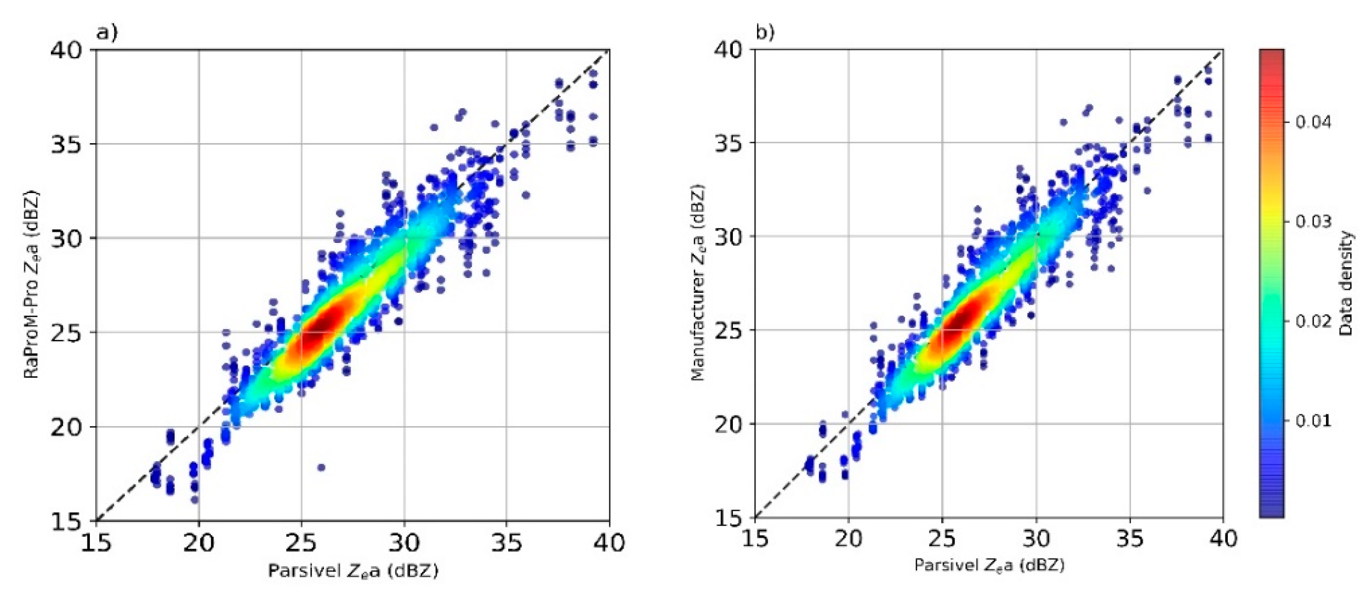
An additional analysis is performed for radar reflectivity comparing the lowest valid radar height bin (from 150 to 200 m above radar level) and the co-located Parsivel disdrometer (
Figure 4) considering 1 min sampling periods. Both radar processing schemes compare very well with Parsivel values, with slight discrepancies that may be explained by instrumental differences—see [
33]. More details about the signal and noise detection scheme can be found in
Appendix A.
3.2. Dealiasing
Spectral reflectivity aliasing occurs when the target returns a signal outside the unambiguous range interval. A systematic method to correct aliasing in MRR-2 was proposed by [
34] and was implemented with some modifications by [
31]. The two methods are based on the estimated velocity parameters calculated from equivalent radar reflectivity in [
35]. Here we propose a different approach, where only signal continuity between vertical levels is used, instead of the parameters estimated in [
35]. According to the manufacturer’s documentation, the radar manufacturer processing is able to detect upward movements of precipitation particles, but in some cases, this detection is not possible, and velocities are aliased.
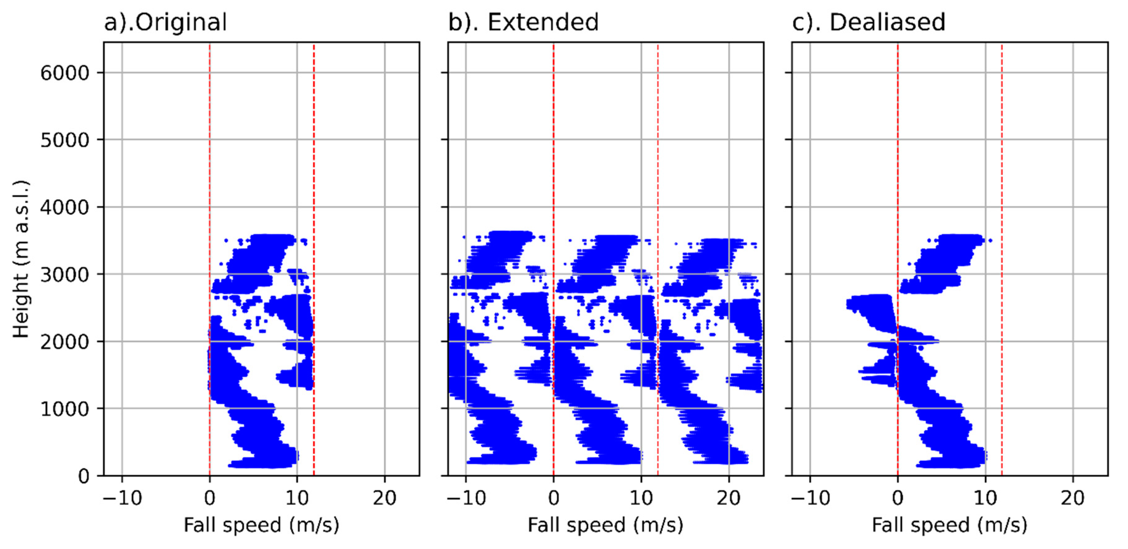
Figure 5 shows an example where the manufacturer velocity spectrum (
Figure 5a) shows a suspicious pattern between 4000 and 5000 m, potentially caused by aliasing. By extending or unfolding the spectra to both sides (
Figure 5b), the vertical continuity of the spectra allows a consistent dealiased spectra profile to be selected (
Figure 5c).
The dealiased spectral reflectivity allows, in this case, to detect upward movements of precipitation particles between 4000 and 5000 m.
Figure 6 shows the corresponding time–height display of this case where RaProM-
Pro detects upward movements, unlike the manufacturer original output, which indicates high downward values. More challenging cases, for example, with convective precipitation and strong windshear might not be detected by the new proposed scheme, which was designed to deal with typical BB conditions (see
Appendix B for more details).
After the dealiasing is applied, different Doppler moments from the spectral reflectivity are computed, including the equivalent radar reflectivity (dBZ), the Doppler velocity (m/s), the spectral width (m/s), the skewness and the kurtosis (Equations (6)–(10)):
where
λ is the radar wavelength, |
K|
2 is the dielectric factor, in this case, liquid water and Δ
v is the Nyquist velocity. Note that the radar reflectivity does not yet consider the possible effects of rainfall attenuation, which is computed in the next subsection.
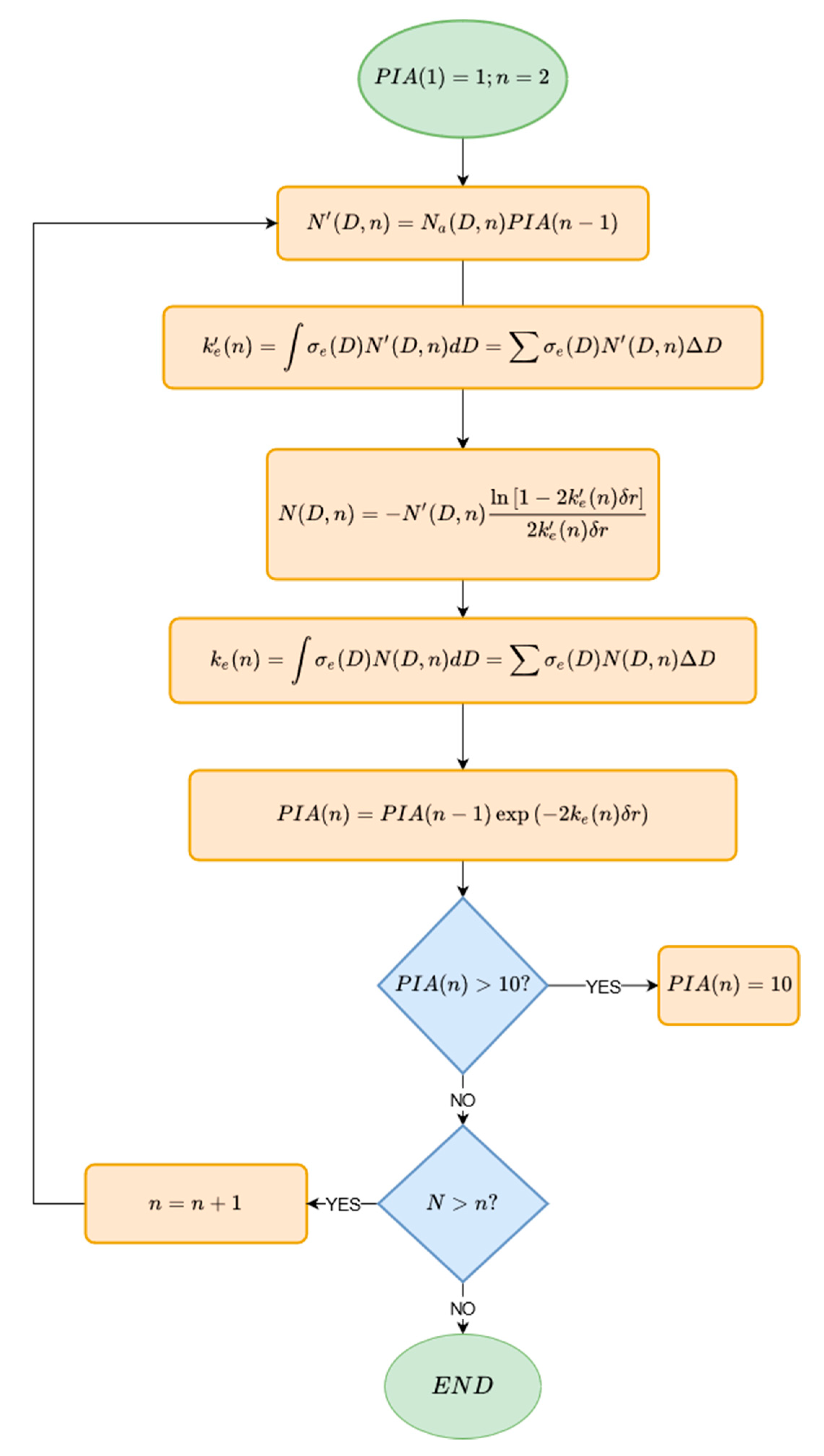
3.3. Attenuation Calculation
Weather radars operating in attenuated frequencies, such as the K-band, may be affected by rainfall attenuation, impacting specific parameters such as radar reflectivity (Z), liquid water content (LWC) and rain rate (RR). Attenuation is calculated to determine the amount of signal loss integrated along a path (in height) by absorption and scattering by precipitating particles. PIA values are computed following an iterative process described in [
36], shown schematically in
Figure 7.
Essentially, drop size distributions
N’(
D,
n), at each level
n, are calculated considering an attenuation factor (the PIA) multiplied by the previous (attenuated) drop size distribution
Na(
D,
n), computed from the Doppler spectra assuming Mie scattering conditions [
37,
38]. As these calculations are only valid for liquid precipitation particles falling at terminal fall speeds, an additional procedure that provides a hydrometeor classification type for each bin height [
31] is applied so that attenuation can be used consistently only for liquid precipitation.
As described in
Figure 7, the maximum PIA value is 10, because for higher values, the scheme may not work properly. If PIA reaches the value of 10, the manufacturer processing stops calculating it for higher range bins. However, RaProM-
Pro assigns a constant value of 10 for internal processing reasons. The final output parameter of PIA in RaProM-
Pro is simply the PIA value expressed in dB (11), called
DBPIA:
The DBPIA calculation is included in RaProM-Pro processing despite it not being applied in the BB determination procedure
3.4. Bright Band Calculation
The new methodology proposed to detect the BB is based on [
39], plus a novel approach considering the vertical variation of the skewness computed from the spectrum Doppler velocity at each height. Skewness provides information about the asymmetry of the fall velocity distribution and indicates that in the BB, snowflakes or ice particles have started to melt [
3,
4,
22]. The change of shape and aerodynamics of the solid particles as they melt modifies the averaged Doppler velocity and the spectrum shape. This change can be observed in the velocity distribution provided by the spectrum reflectivity at each height, where the maximum value changes from being tilted to the right to being tilted to the left, which implies a change of sign of the skewness.
Figure 8 shows an example observed by the MRR-
Pro, highlighting the different spectra shape above, within and below the BB calculated by RaProM-
Pro.
The change in the shape of the spectra is clearly visible in
Figure 8, where the progressive appearance of raindrops at the expense of melted solid particles (
Figure 8b) modifies the Doppler velocity spectra, widening it to the right due to higher fall speeds. This leads to a symmetric or slightly right-skewed spectrum distribution, which implies a change of the skewness from negative to positive values. Determining the height where the skewness sign changes is thus a key feature to obtain the height of the BB.
The method proposed is detailed in the flowchart shown in
Figure 9, which describes, first, the BB detection approach, based on [
39], and then the BB characterisation, which computes the BB top and the BB bottom. The remaining BB feature, the BBpeak, is the level located between the BB bottom and the BB top, where the skewness is maximum and should be close to the melting level. An additional checking is performed to remove BB detections of virga cases, simply verifying that precipitation reaches the ground.
The procedure is applied to each MRR-
Pro vertical profile (in our case, available every 10 s). Then the results (BB top, BB peak and BB bottom) are smoothed temporally, considering a generalised exponential moving average [
40], allowing a more continuous signal of BB characteristics, but keeping the original temporal resolution. Note that the current implementation of the scheme detects the lowest BB present in a vertical profile.
4. Results
The methodology presented in the previous section is illustrated in
Figure 10, displaying both radiosonde data (
Figure 10a) and MRR-
Pro data (
Figure 10b) for a clear BB case. The figure shows the sounding profiles of dry-bulb, wet-bulb and dew point temperature (
Figure 10a) recorded the 31 March 2020 at 12 UTC and radar equivalent reflectivity Ze from MRR-
Pro and Parsivel observations; the latter was plotted at the lowest height level and resampled at a 10 s resolution to match MRR-
Pro observations, from 12 to 15 UTC (
Figure 10b). The sounding plot panel explicitly shows that the 0 °C wet-bulb temperature is relatively lower than the freezing level (0 °C dry-bulb temperature) due to low saturation. The wind profile is also plotted, showing west wind components below the BB, which is consistent with the precipitation fall streaks visible from the BB.
Figure 10b shows consistent reflectivity values of ground measures from Parsivel and the first lowest valid height bin from the radar, for example, the alternating maxima and minima reflectivity columns. The 12 UTC melting levels and 0 °C wet-bulb temperature levels obtained with the sounding match the detected BB top and BB bottom well, respectively. This example illustrates well the ability of the new methodology to provide a temporal evolution of the BB details with a 10 s resolution.
The results are presented in the following subsections, considering three different statistical comparisons. The first one is performed comparing the manufacturer’s BB product and the proposed methodology. The second and third subsections compare, respectively, the new methodology and the original manufacturer product, with radio sounding observations.
4.1. Manufacturer ML Height vs. RaProM-Pro BBpeak Height
The previous example is the starting point to assess differences between the manufacturer’s BB product and the new proposed methodology.
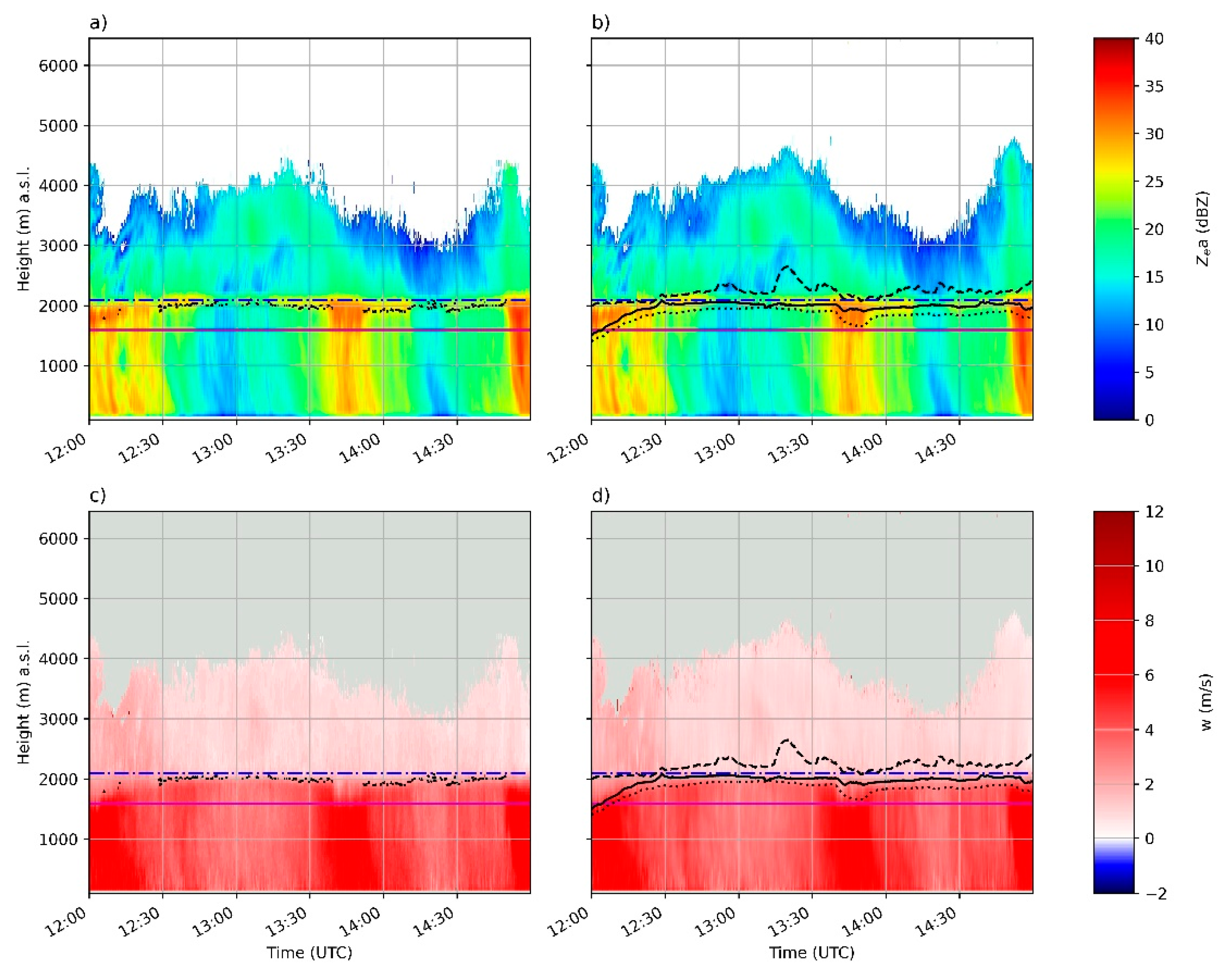
Figure 11 shows radar reflectivity and Doppler velocity profiles processed with each methodology, also including the ML manufacturer’s product and the proposed BB product. In this case, the melting layer heights computed by the manufacturer are always plotted between the estimated BB top and BB bottom, which provide a more complete description of the BB. Additionally, RaProM-
Pro offers a more detailed description of the precipitation field (better depiction of contours and inclusion of additional weather echoes) around 15 UTC, particularly above the BB (from 4000 to 5000 m) thanks to the new noise and peak detection methodology.
A quantitative analysis is provided by comparing the melting layer (ML) height provided by the manufacturer and the
BBpeak height calculated with RaProM-
Pro, given by:
The ML product is calculated using an Artificial Intelligence approach [
41], providing probability values; a probability greater than 0.75 is considered a reliable ML height determination, being the maximum probability of the selected height for the melting level. The BB peak has been described in
Section 3.
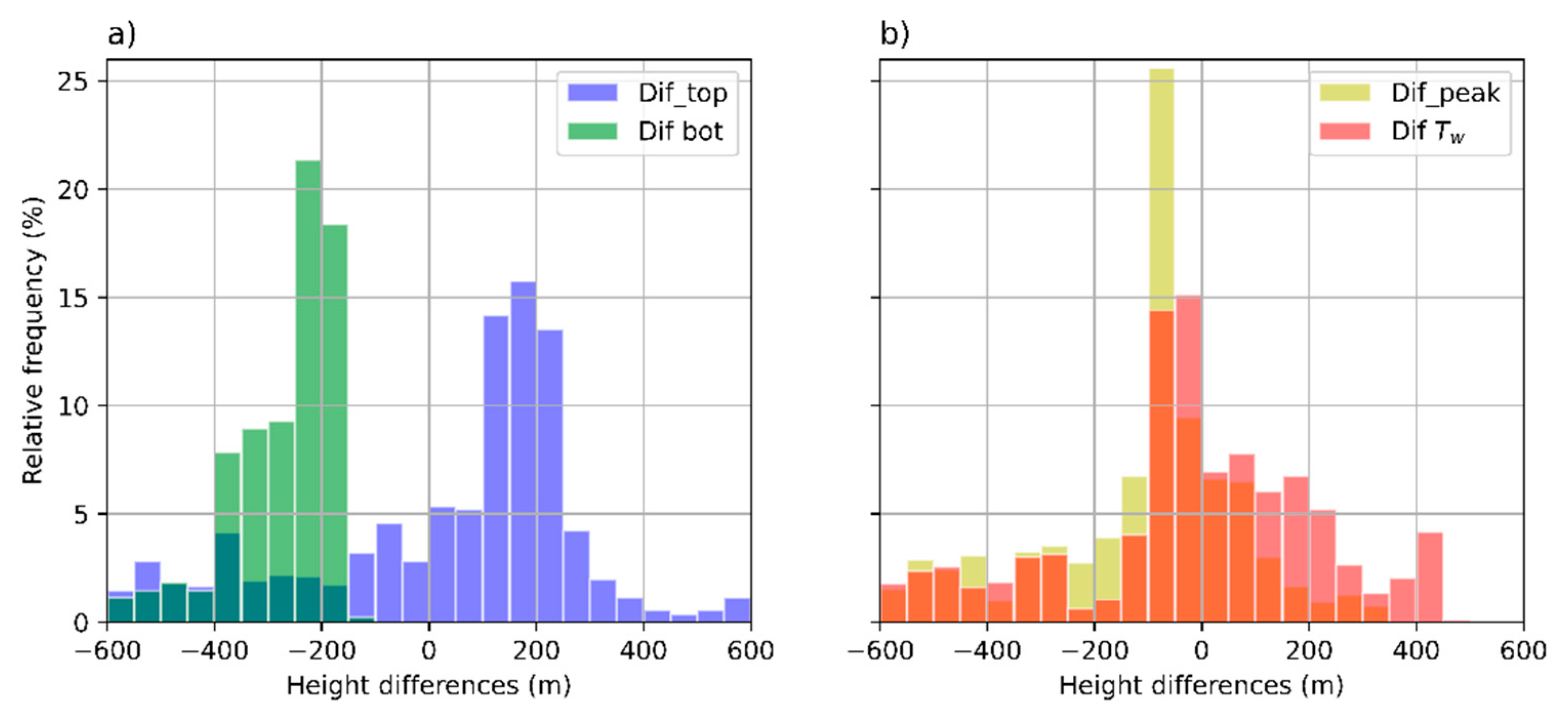
Figure 12 shows a histogram of
Diff_ML for 39 days, selecting a time window of ±1 h from the sounding launch, resulting in around 2600 cases. It displays a nearly symmetrical distribution pattern with a single-mode centred in the second negative class (from −50 to −100 m), indicating that the manufacturer’s ML height is slightly lower than the
BBpeak (the averaged value of
Diff_ML is −89 m and the standard deviation is 180 m). More than 80% of cases do not exceed 200 m, and the tails of the distribution fall quickly, which despite some differences, reach values higher than 400 m.
4.2. Sounding Observations vs. RaProM-Pro BB Levels
The 0 °C dry-bulb temperature level (freezing level, hereafter h0) and the 0 °C wet-bulb temperature level (hereafter hw,0) are compared here with the BBtop, BBpeak and BBbot heights. We consider the same 39 days studied in the previous subsection, with the same time intervals of ±1 h from the sounding launch time to minimise spurious differences caused by rapidly changing BB heights, leading to around 5327 cases.
The evaluation is performed using the parameters
Diff_top,
Diff_bot,
Diff_peak and
Diff_Tw defined as:
where
BBtop,
BBbot and
BBpeak are the heights from the BB top, BB bottom and BB peak, respectively. Note that a priori,
Diff_top should be close to 0 as solid particles begin to melt when they reach the melting level,
Diff_bot should be greater than 0, as it takes some time to completely melt all solid particles and, by definition,
Diff_peak, should be between
Diff_top and
Diff_bot. Regarding the expected value of
Diff_Tw, the recent study of [
42] indicated that
BBpeak heights were very similar to
hw,0, so a value close to 0 would be consistent with that result.
Figure 13a shows histograms of
Diff_top and
Diff_bot, indicating similar patterns but centred, respectively, below and above
h0:
BBtop mode is between 150 and 200 m, and
BBbot is between −250 and −2000 m. The fact that
BBtop occurs mostly above
h0 (so it is not close to 0 as initially expected) can be explained by the tendency of solid particles to increase aggregation just above the melting level, producing larger snowflakes and reducing the number of smaller particles [
6]. This would lead to a change in the skewness spectrum, which would be detected by the proposed methodology as the
BBtop. On the other hand, the mode value of
Diff_bot found is reasonable, compared with previous existing studies, such as [
4].
Figure 13b shows that the
Diff_peak histogram presents a similar pattern to
Diff_top and
Diff_bot, but, as expected, the mode value, more pronounced (corresponding to a more leptokurtic distribution), is centred between the previous two modes, close to 0. Finally,
Diff_Tw presents a slightly thicker mode, with a maximum between −50 and 0 m, which is just one class below the
Diff_peak mode.
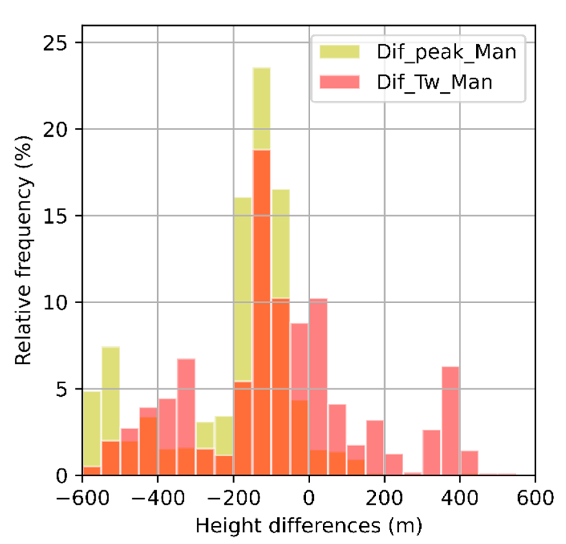
4.3. Sounding Observations vs. Manufacturer ML Levels
In this subsection, the same analysis performed in
Section 4.2 is applied to the manufacturer’s ML product for 1749 cases detected in the same time period considered above. However, in this case, no BB top nor bottom are considered; only a BB peak is given here by the maximum probability of the ML height product (exceeding 75% as mentioned earlier), denoted as
MLmax. We computed the differences between the
MLmax and sounding-derived zero dry and wet-bulb temperature heights
(Diff_peak_Man and
Diff_Tw_Man respectively), given by:
The distributions of these variables are displayed in
Figure 14, similarly to
Figure 13b. Both variables show similar patterns and a common main mode corresponding to the same class of height differences (−150 to −100 m) and are relatively wide (three to four different height classes). Secondary modes exceeding 5% relative frequencies are found around −300 and +400 m for
Diff_peak_Man and around −500 m for
Diff_Tw_Man.
5. Discussion
According to the results shown in the previous section, the proposed BB detection and characterisation method provides some advantages.
Firstly, the new dealiasing scheme presents an improvement in some cases where the manufacturer standard processing fails. Despite the fact that the new dealiasing cannot handle very complex cases, such as those found on convective precipitation with intense turbulence, environments favourable to BB conditions, with moderate updrafts, are reasonably well identified, improving the original manufacturer’s software capabilities.
Secondly, the BB detection proposed, when compared to radiosounding derived zero dry and wet-bulb temperatures, provide narrower difference height distributions compared to those obtained with the manufacturer’s ML product. This suggests that, despite both schemes performing similarly, the proposed methodology gives lower differences compared to the observed freezing level. Moreover, the new method gives explicit information about the BB top and bottom, information not available from the ML manufacturer’s product, and the number of detections is considerably higher (5327 vs. 1749 in the period examined).
Despite improvements in the dealiasing approach, limitations of the proposed method include the inability to correct fully folded velocity profiles and also convection with strong windshear. However, these conditions do not typically produce BBs. On the other hand, strong windshear with stratiform precipitation, leading to tilted precipitation streaks, might be a problem for the BB scheme because it examines single radar vertical profiles. Moreover, the proposed scheme cannot handle either multiple BB cases as only the lowest BB can be detected. In any case, the new method based on the vertical variability of the Doppler speed skewness provides a good basis for the further development of more sophisticated BB detection methods.
6. Summary and Conclusions
The work presents a new methodology to process spectral raw reflectivity data from a K-band vertically pointing Doppler radar, implemented for the Metek MRR-Pro system, and called RaProM-Pro, which is freely available. RaProM-Pro can be used complementary with the manufacturer’s software and provides additional features, such as an improved signal and noise detection scheme, an advanced dealiasing method and a new Bright Band product (including top, peak and bottom levels).
The study illustrates the advantages of RaProM-Pro, such as the capability to detect weaker signals or the robust detection of updrafts thanks to a novel dealiasing scheme. The derived parameters, such as radar reflectivity, mostly match the values provided by the manufacturer (R2 of 0.992) and is also consistent with independent observations from co-located disdrometer data. The new Bright Band product, based on changes of the skewness of spectral Doppler velocities, compares favourably with the manufacturer’s Melting Level product and also with collocated radio sounding observations, both qualitatively in selected examples and quantitatively, as revealed by a study considering 39 days.
Based on the current results, future work is planned to perform a long-term study of BB features in more detail, including BB occurrence, height, thickness and atmospheric conditions (dry and moist BBs).
The methodology can be used for both research and operational applications and could be adapted to other vertically pointing radars. RaProM-Pro is written in Python and is freely available at the GitHub repository.
Author Contributions
Conceptualisation, A.G.-B. and J.B.; methodology, A.G.-B. and J.B.; software, A.G.-B. and S.G.; data curation, A.G.-B.; writing—original draft preparation, A.G.-B. and J.B.; writing—review and editing, A.G.-B., B.J, S.G., M.U. and B.C. All authors have read and agreed to the published version of the manuscript.
Funding
This research was partly funded by the project “Analysis of Precipitation Processes in the Eastern Ebro Subbasin” (WISE-PreP, RTI2018-098693-B-C32, MINECO/FEDER) and the Water Research Institute (IdRA) of the University of Barcelona.
Data Availability Statement
The proposed methodology coded as a Python program is available at the GitHub repository (
https://github.com/AlbertGBena/RaProM-Pro.git). Radiosonde data are available from the Meteorological Service of Catalonia (meteo.cat) and MRR-
Pro and Parsivel data are available from the authors upon request.
Acknowledgments
Radiosonde data of the Meteorological Service of Catalonia were used in this study.
Conflicts of Interest
The authors declare no conflict of interest.
Appendix A
This Appendix provides additional information about the new processing methodology regarding noise and signal detection introduced in
Section 3.1. Based on 3 h of precipitation data recorded from 12 to 15 UTC 31 March 2020 (
Figure 11), 138,240 points (height gates) were examined.
Figure A1 shows a mask of three possible cases regarding the signal and noise detection of each method: gates (pixels) with the signal detected by both methods, gates with noise detected by both methods and pixels detected only by one of the methods.
Figure A1.
Signal and noise detection comparison between manufacturer and RaProm-Pro schemes: pixels with the signal detected by both methods (white), noise detected by both methods (grey), pixels detected only by the manufacturer (a) and RaProm-Pro (b) methods (red). The data were recorded from 12 to 15 UTC, 31 March 2020.
It is clear that both methods perform similarly, as most signal and noise detections are identical; only a small fraction, close or at the precipitation contours, is detected differently, being RaProM-
Pro a bit more sensitive (about 2.8% more signal detection than the manufacturer’s method, as listed in
Table A1).
Table A1.
Signal and noise gates detected by manufacturer versus RaProM-Pro methods.
Table A1.
Signal and noise gates detected by manufacturer versus RaProM-Pro methods.
| Cases (12 to 15 UTC 31 March 2020) | Number | % |
|---|
| Total number of gates | 138,240 | 100.00 |
| Noise gates identified both by manufacturer and RaProM-Pro | 57,654 | 41.71 |
| RaProM-Pro signal gates identified as noise gates by manufacturer | 4062 | 2.94 |
| Manufacturer signal gates identified as noise gates by RaProM-Pro | 166 | 0.12 |
| Signal gates identified both by manufacturer and RaProM-Pro | 76,358 | 55.23 |
Appendix B
This Appendix provides more details about the dealiasing scheme proposed.
The dealiasing scheme is based on the original work by [
43,
44], and it has been tested for 39 2 h events with precipitation and radiosounding data with the aim to apply it for BB detection. Other more challenging situations, such as convective precipitation with windshear or strong turbulence, where typically BB is not present, may not produce good results.
Figure A2 shows one of these cases, recorded on 27 July 2019, displaying the Doppler vertical velocity provided by the manufacturer and the new dealiasing scheme.
Figure A3 (analogous to the simpler case shown in
Figure 5) illustrates the steps of the dealiasing applied. Two basic concepts are considered in the scheme: Doppler bin clustering (of precipitation and non-precipitation blocks) and vertical continuity of precipitation blocks.
Figure A2.
Time–height display of the Doppler velocity (positive values indicate downward direction) obtained with MRR-Pro on 27 July 2019, processed with: (a) the manufacturer’s software, (b). RaProM-Pro. Panels (c,d) show zooms of the previous images, from 10:10 to 10:20 UTC.
Figure A2.
Time–height display of the Doppler velocity (positive values indicate downward direction) obtained with MRR-Pro on 27 July 2019, processed with: (a) the manufacturer’s software, (b). RaProM-Pro. Panels (c,d) show zooms of the previous images, from 10:10 to 10:20 UTC.
Figure A3.
Doppler velocity dealiasing applied with RaProm-Pro compared to the original data (27 July 2019, 10:16:30 UTC). Original Doppler spectra profile (a), extended Doppler spectra profile (b) and final dealiased Doppler spectra profile (c).
Figure A3.
Doppler velocity dealiasing applied with RaProm-Pro compared to the original data (27 July 2019, 10:16:30 UTC). Original Doppler spectra profile (a), extended Doppler spectra profile (b) and final dealiased Doppler spectra profile (c).
For each height, two Doppler bin groups are identified: blocks of continuous precipitation bins and blocks of non-precipitation bins (hereafter gaps) (
Figure A3a). Then, the spectra are extended to both sides of the Nyquist velocity interval, i.e., considering stronger fall speeds (adding to the right of the original spectra the spectra immediately above the central one) or upward speeds (adding to the left of the original spectra the spectra immediately below the central one). A new grouping of Doppler bins is applied to the extended spectra, providing new precipitation blocks and gaps (
Figure A3b). Now three options are possible to select the dealiased velocity profile, and we assume that only one, for each height, is valid. Starting from the second lowest valid level to higher ones, the selection criteria is that the average velocity of the level considered is closest to the average velocity of the level below (
Figure A3c).
In this convective case, the results seem reasonable for aliasing found from 1500 to ca. 2500 m ASL, but it is not so clear for heights above 2500 m ASL.
References
- Tapiador, F.J.; Sánchez, J.L.; García-Ortega, E. Empirical values and assumptions in the microphysics of numerical models. Atmos. Res. 2019, 215, 214–238. [Google Scholar] [CrossRef]
- Gray, W.R.; Cluckie, D.I.; Griffith, R.J. Aspects of melting and the radar bright band. Meteorol. Appl. 2001, 8, 371–379. [Google Scholar] [CrossRef]
- White, A.B.; Gottas, D.J.; Strem, E.T.; Ralph, F.M.; Neiman, P.J. An Automated Brightband Height Detection Algorithm for Use with Doppler Radar Spectral Moments. J. Atmos. Ocean. Technol. 2002, 19, 687–697. [Google Scholar] [CrossRef] [Green Version]
- Fabry, F.; Zawadzki, I. Long-term radar observations of the melting layer of precipitation and their interpretation. J. Atmos. Sci. 1995. [Google Scholar] [CrossRef]
- Fabry, F. Radar Meteorology Principles and Practice; Cambridge University Press: Cambridge, UK, 2018; ISBN 9781108460392. [Google Scholar]
- Heymsfield, A.J.; Bansemer, A.; Poellot, M.R.; Wood, N. Observations of Ice Microphysics through the Melting Layer. J. Atmos. Sci. 2015, 72, 2902–2928. [Google Scholar] [CrossRef]
- Bordoy, R.; Bech, J.; Rigo, T.; Pineda, N. Analysis of a method for radar rainfall estimation considering the freezing level height. Tethys J. Weather Clim. West. Mediterr. 2010, 25–39. [Google Scholar] [CrossRef]
- Hall, W.; Rico-Ramirez, M.A.; Krämer, S. Classification and correction of the bright band using an operational C-band polarimetric radar. J. Hydrol. 2015, 531, 248–258. [Google Scholar] [CrossRef] [Green Version]
- Sánchez-Diezma, R.; Zawadzki, I.; Sempere-Torres, D. Identification of the bright band through the analysis of volumetric radar data. J. Geophys. Res. Atmos. 2000. [Google Scholar] [CrossRef]
- Bech, J.; Pineda, N.; Rigo, T.; Aran, M. Remote sensing analysis of a Mediterranean thundersnow and low-altitude heavy snowfall event. Atmos. Res. 2013, 123, 305–322. [Google Scholar] [CrossRef]
- Casellas, E.; Bech, J.; Veciana, R.; Pineda, N.; Rigo, T.; Miró, J.R.; Sairouni, A. Surface precipitation phase discrimination in complex terrain. J. Hydrol. 2021, 592, 125780. [Google Scholar] [CrossRef]
- Casellas, E.; Bech, J.; Veciana, R.; Pineda, N.; Miró, J.R.; Moré, J.; Rigo, T.; Sairouni, A. Nowcasting the precipitation phase combining weather radar data, surface observations, and NWP model forecasts. Q. J. R. Meteorol. Soc. 2021, 147, 3135–3153. [Google Scholar] [CrossRef]
- Demir, I.; Krajewski, W.F. Towards an integrated Flood Information System: Centralized data access, analysis, and visualization. Environ. Model. Softw. 2013, 50, 77–84. [Google Scholar] [CrossRef]
- Rossa, A.; Haase, G.; Keil, C.; Alberoni, P.; Ballard, S.; Bech, J.; Germann, U.; Pfeifer, M.; Salonen, K. Propagation of uncertainty from observing systems into NWP: COST-731 Working Group 1. Atmos. Sci. Lett. 2010, 11, 145–152. [Google Scholar] [CrossRef] [Green Version]
- Seo, B.C.; Krajewski, W.F. Statewide real-time quantitative precipitation estimation using weather radar and NWP model analysis: Algorithm description and product evaluation. Environ. Model. Softw. 2020, 132, 104791. [Google Scholar] [CrossRef]
- Ryzhkov, A.; Zhang, P.; Reeves, H.; Kumjian, M.; Tschallener, T.; Trömel, S.; Simmer, C. Quasi-Vertical Profiles—A New Way to Look at Polarimetric Radar Data. J. Atmos. Ocean. Technol. 2016, 33, 551–562. [Google Scholar] [CrossRef]
- Tokay, A.; Hartmann, P.; Battaglia, A.; Gage, K.S.; Clark, W.L.; Williams, C.R. A field study of reflectivity and Z-R relations using vertically pointing radars and disdrometers. J. Atmos. Ocean. Technol. 2009. [Google Scholar] [CrossRef]
- Das, S.; Shukla, A.K.; Maitra, A. Investigation of vertical profile of rain microstructure at Ahmedabad in Indian tropical region. Adv. Sp. Res. 2010, 45, 1235–1243. [Google Scholar] [CrossRef]
- Massmann, A.K.; Minder, J.R.; Garreaud, R.D.; Kingsmill, D.E.; Valenzuela, R.A.; Montecinos, A.; Fults, S.L.; Snider, J.R. The Chilean Coastal Orographic Precipitation Experiment: Observing the Influence of Microphysical Rain Regimes on Coastal Orographic Precipitation. J. Hydrometeorol. 2017, 18, 2723–2743. [Google Scholar] [CrossRef]
- Pfaff, T.; Engelbrecht, A.; Seidel, J. Detection of the bright band with a vertically pointing K-band radar. Meteorol. Z. 2014, 23, 527–534. [Google Scholar] [CrossRef]
- Wang, H.; Lei, H.; Yang, J. Microphysical processes of a stratiform precipitation event over eastern China: Analysis using Micro Rain Radar data. Adv. Atmos. Sci. 2017. [Google Scholar] [CrossRef]
- Li, H.; Moisseev, D. Two Layers of Melting Ice Particles Within a Single Radar Bright Band: Interpretation and Implications. Geophys. Res. Lett. 2020, 47, e2020GL087499. [Google Scholar] [CrossRef]
- Romatschke, U. Melting Layer Detection and Observation with the NCAR Airborne W-Band Radar. Remote Sens. 2021, 13, 1660. [Google Scholar] [CrossRef]
- Benarroch, A.; Siles, G.A.; Riera, J.M.; Perez-Pena, S. Heights of the 0 °C Isotherm and the Bright Band in Madrid: Comparison and Variability. In Proceedings of the 14th European Conference on Antennas and Propagation, EuCAP 2020, Copenhagen, Denmark, 15–20 March 2020. [Google Scholar]
- Lin, D.; Pickering, B.; Neely, R.R., III. Relating the Radar Bright Band and Its Strength to Surface Rainfall Rate Using an Automated Approach. J. Hydrometeorol. 2020, 21, 335–353. [Google Scholar] [CrossRef]
- Alpers, W.; Zhao, Y.; Mouche, A.A.; Chan, P.W. A note on radar signatures of hydrometeors in the melting layer as inferred from Sentinel-1 SAR data acquired over the ocean. Remote Sens. Environ. 2021, 253, 112177. [Google Scholar] [CrossRef]
- Arulraj, M.; Barros, A.P. Automatic detection and classification of low-level orographic precipitation processes from space-borne radars using machine learning. Remote Sens. Environ. 2021, 257, 112355. [Google Scholar] [CrossRef]
- Peters, G.; Fischer, B.; Andersson, T. Rain observations with a vertically looking Micro Rain Radar (MRR). Boreal Environ. Res. 2002, 7, 353–362. [Google Scholar]
- Tokay, A.; Wolff, D.B.; Petersen, W.A. Evaluation of the New Version of the Laser-Optical Disdrometer, OTT Parsivel2. J. Atmos. Ocean. Technol. 2014, 31, 1276–1288. [Google Scholar] [CrossRef]
- Metek MRR-Pro. Description of Products. Valid for MRR-PRO Firmware VS ≥ 01; Metek Meteorologische Messtechnik GmbH: Elmshorn, Germany, 2010. [Google Scholar]
- Garcia-Benadi, A.; Bech, J.; Gonzalez, S.; Udina, M.; Codina, B.; Georgis, J.F. Precipitation type classification of Micro Rain Radar data using an improved Doppler spectral processing methodology. Remote Sens. 2020, 12, 4113. [Google Scholar] [CrossRef]
- Hildebrand, P.H.; Sekhon, R.S. Objective Determination of the Noise Level in Doppler Spectra. J. Appl. Meteorol. 1974, 13, 808–811. [Google Scholar] [CrossRef] [Green Version]
- Adirosi, E.; Baldini, L.; Tokay, A.L.I. Rainfall and DSD parameters comparison between Micro Rain Radar, two-dimensional video and Parsivel2 disdrometers, and S-band dual-polarization radar. J. Atmos. Ocean. Technol. 2020. [Google Scholar] [CrossRef]
- Maahn, M.; Kollias, P. Improved Micro Rain Radar snow measurements using Doppler spectra post-processing. Atmos. Meas. Tech. 2012, 5, 2661–2673. [Google Scholar] [CrossRef] [Green Version]
- Atlas, D.; Srivastava, R.C.; Sekhon, R.S. Doppler radar characteristics of precipitation at vertical incidence. Rev. Geophys. 1973, 11, 1–35. [Google Scholar] [CrossRef]
- Peters, G.; Fischer, B.; Clemens, M. Rain Attenuation of Radar Echoes Considering Finite-Range Resolution and Using Drop Size Distributions. J. Atmos. Ocean. Technol. 2010, 27, 829–842. [Google Scholar] [CrossRef]
- Prahl, S. Miepython. Available online: https://miepython.readthedocs.io/ (accessed on 1 July 2021).
- Wiscombe, W.J. Improved Mie scattering algorithms. Appl. Opt. 1980, 19, 1505–1509. [Google Scholar] [CrossRef]
- Cha, J.-W.; Chang, K.-H.; Yum, S.S.; Choi, Y.-J. Comparison of the bright band characteristics measured by Micro Rain Radar (MRR) at a mountain and a coastal site in South Korea. Adv. Atmos. Sci. 2009, 26, 211–221. [Google Scholar] [CrossRef]
- Nakano, M.; Takahashi, A.; Takahashi, S. Generalized exponential moving average (EMA) model with particle filtering and anomaly detection. Expert Syst. Appl. 2017, 73, 187–200. [Google Scholar] [CrossRef]
- Brast, M.; Markmann, P. Detecting the Melting Layer with a Micro Rain Radar Using a Neural Network Approach. Atmos. Meas. Tech. 2020, 13, 6645–6656. [Google Scholar] [CrossRef]
- Lee, J.-E.; Jung, S.-H.; Kwon, S. Characteristics of the Bright Band Based on Quasi-Vertical Profiles of Polarimetric Observations from an S-Band Weather Radar Network. Remote Sens. 2020, 12, 4061. [Google Scholar] [CrossRef]
- Kneifel, S.; Maahn, M.; Peters, G.; Simmer, C. Observation of snowfall with a low-power FM-CW K-band radar (Micro Rain Radar). Meteorol. Atmos. Phys. 2011. [Google Scholar] [CrossRef] [Green Version]
- Kneifel, S.; Kulie, M.S.; Bennartz, R. A triple-frequency approach to retrieve microphysical snowfall parameters. J. Geophys. Res. Atmos. 2011, 116, D11203. [Google Scholar] [CrossRef] [Green Version]
Figure 1.
Description of selected parameters contained in the manufacturer’s netcdf file. Parameters in green are required by the proposed methodology implemented in RaProM-Pro.
Figure 1.
Description of selected parameters contained in the manufacturer’s netcdf file. Parameters in green are required by the proposed methodology implemented in RaProM-Pro.
Figure 2.
Flowchart of the new processing methodology.
Figure 2.
Flowchart of the new processing methodology.
Figure 3.
Scatter plots comparing the manufacturer and the RaProM-Pro processing. (a) Equivalent radar reflectivity, (b) signal-to-noise ratio and (c) Doppler vertical velocity. Data were recorded on 21 April 2020 from 10 h to 14 h UTC.
Figure 3.
Scatter plots comparing the manufacturer and the RaProM-Pro processing. (a) Equivalent radar reflectivity, (b) signal-to-noise ratio and (c) Doppler vertical velocity. Data were recorded on 21 April 2020 from 10 h to 14 h UTC.
Figure 4.
Scatter plots of equivalent radar reflectivity of the lowest valid height bin (150 to 200 m above radar level) of (a) RaProM-Pro and (b) the manufacturer processing vs. the Parsivel disdrometer located at the radar level. Coefficients of determination are equal to 0.878 (RaProM-Pro) and 0.879 (manufacturer) for 1195 samples. Data were recorded on 21 April 2020 from 10 h to 14 h UTC.
Figure 5.
Example of Doppler velocity dealiasing applied with RaProM-Pro compared to the original data (16 May 2020, 13:45 UTC). Original Doppler spectra profile (a), extended Doppler spectra profile (b) and final dealiased Doppler spectra profile (c).
Figure 5.
Example of Doppler velocity dealiasing applied with RaProM-Pro compared to the original data (16 May 2020, 13:45 UTC). Original Doppler spectra profile (a), extended Doppler spectra profile (b) and final dealiased Doppler spectra profile (c).
Figure 6.
Time–height display of Doppler vertical velocity (positive values indicate downward direction) obtained with MRR-Pro on 16 May 2020 processed with: (a). The manufacturer’s software, (b). RaProM-Pro, which includes a new dealiasing scheme.
Figure 6.
Time–height display of Doppler vertical velocity (positive values indicate downward direction) obtained with MRR-Pro on 16 May 2020 processed with: (a). The manufacturer’s software, (b). RaProM-Pro, which includes a new dealiasing scheme.
Figure 7.
PIA calculation flow chart adapted from [
36].
N’(
D,
n) and
Na(
D,
n) are, respectively, the drop size distribution and the attenuated drop size distribution;
ke is the specific rain attenuation and
σe is the single-particle extinction coefficient, calculated with the Mie theory.
Figure 7.
PIA calculation flow chart adapted from [
36].
N’(
D,
n) and
Na(
D,
n) are, respectively, the drop size distribution and the attenuated drop size distribution;
ke is the specific rain attenuation and
σe is the single-particle extinction coefficient, calculated with the Mie theory.
Figure 8.
Examples of the Doppler velocity distribution (redsolid line) and fitted normal distribution calculated with the same average Doppler velocity and spectral width (blue dashed line) obtained at three different heights: (a). above the Bright Band (2350 m ASL), (b). within the Bright Band (1900 m ASL) and (c). below the Bright Band (1800 m ASL), on 5 December 2019. Skewness values (Sk) are given for each height.
Figure 9.
Bright Band (BB) detection and calculation of BB bottom (BBbot) and BB top (BBtop). The Deltah parameter is equal to the vertical resolution of the radar data.
Figure 9.
Bright Band (BB) detection and calculation of BB bottom (BBbot) and BB top (BBtop). The Deltah parameter is equal to the vertical resolution of the radar data.
Figure 10.
(a). Sounding profiles of dry-bulb (T), wet-bulb (Tw) and dew point (Td) temperatures, also showing the 0 °C, −10 °C, −20 °C dry-bulb and 0 °C wet-bulb temperature levels and the wind profile, corresponding to 31 March 2020 12 UTC, (b). Radar equivalent reflectivity time–height display from MRR-Pro and Parsivel observations, the latter is plotted at the low height level, from 12 to 15 UTC 31 March 2020.
Figure 11.
Time–height display of equivalent radar reflectivity—top row, panels (a,b) and Doppler velocity—bottom row, panels (c,d) calculated with the manufacturer’s software (first column) and RaProM-Pro (second column). First and second column show, respectively, the melting level detected by the manufacturer (black dots) and the BB top, BB peak and BB bottom (dashed, continuous, and dotted black lines). The data corresponds to 31 March 2020.
Figure 12.
Histogram of differences between the melting level height provided by the manufacturer and the Bright Band peak height from RaProM-Pro. The height bin resolution is equal to the histogram class bin, 50 m.
Figure 12.
Histogram of differences between the melting level height provided by the manufacturer and the Bright Band peak height from RaProM-Pro. The height bin resolution is equal to the histogram class bin, 50 m.
Figure 13.
(a). Histograms of the differences between Bright Band top and Bright Band bottom heights and the sounding-derived freezing levels Diff_top (blue) and Diff_bot (green), respectively, and (b). histograms of differences between Bright Band peak height and the sounding-derived height of zero wet-bulb temperature, Diff_Tw (red) and differences between Bright Band peak height and the freezing level, Diff_peak (yellow). Values are analysed around ±1.5 h from the sounding launch time.
Figure 14.
As in
Figure 13b but for the manufacturer’s ML product.
Figure 14.
As in
Figure 13b but for the manufacturer’s ML product.
Table 1.
MRR-Pro configuration parameters used in this study.
Table 1.
MRR-Pro configuration parameters used in this study.
| Definition | Parameter | Units | Values |
|---|
| Number of Doppler bins | M | -- | 64 |
| Number of height bins | N | -- | 128 |
| Temporal resolution | Ti | s | 10 |
| Height bin resolution | Δh | m | 50 |
| Nyquist Velocity | vny | m·s−1 | 12 |
| Interval of velocity | Δv | m·s−1 | 0.19 |
| Publisher’s Note: MDPI stays neutral with regard to jurisdictional claims in published maps and institutional affiliations. |
© 2021 by the authors. Licensee MDPI, Basel, Switzerland. This article is an open access article distributed under the terms and conditions of the Creative Commons Attribution (CC BY) license (https://creativecommons.org/licenses/by/4.0/).


