Vector Fuzzy c-Spherical Shells (VFCSS) over Non-Crisp Numbers for Satellite Imaging

Abstract

The conventional fuzzy c-spherical shells (FCSS) clustering model is extended to cluster shells involving non-crisp numbers, in this paper. This is achieved by a vectorized representation of distance, between two non-crisp numbers like the crisp numbers case. Using the proposed clustering method, named vector fuzzy c-spherical shells (VFCSS), all crisp and non-crisp numbers can be clustered by the FCSS algorithm in a unique structure. Therefore, we can implement FCSS clustering over various types of numbers in a unique structure with only a few alterations in the details used in implementing each case. The relations of VFCSS applied to crisp and non-crisp (containing symbolic-interval, LR-type, TFN-type and TAN-type fuzzy) numbers are presented in this paper. Finally, simulation results are reported for VFCSS applied to synthetic LR-type fuzzy numbers; where the application of the proposed method in real life and in geomorphology science is illustrated by extracting the radii of circular agricultural fields using remotely sensed images and the results show better performance and lower cost computational complexity of the proposed method in comparison to conventional FCSS.

1. Introduction

Use of clustering models is a wide field of research in image processing and pattern recognition and they have been applied in different areas such as business, geology, engineering systems, etc. [1,2,3]. The objective of clustering is to explore the structure of the data and to partition the data set into groups with similar individuals. While the proposed method in this paper is objective-function based, generally clustering models may be objective-function, hierarchical or heuristic based. Hard clustering methods restrict each point of the data set to exactly one cluster [4]. Since Zadeh [5] presented fuzzy sets which introduce the idea of partial membership of belonging defined by a membership function, fuzzy clustering has been applied in various areas. After that, research in this field has been extended to apply fuzzy states to crisp cases. In the literature on fuzzy clustering, the fuzzy c-mean (FCM) clustering algorithms are the best-known methods [2,6]. Hadi et al. [7,8,9] presented some models to apply the FCM clustering model to crisp and non-crisp numbers. Using these models, the FCM can be stated in a single structure like the conventional FCM case. Sasha and Das [10] proposed an axiomatic extension of the possibilistic fuzzy clustering model in three directions: joint contribution function, choice of the dissimilarity measure, and the penalty function. Yu et al. [11] proposed a Suppressed Possibilistic C-Means (S-PCM) clustering model by creating a suppressed competitive learning approach into the Possibilistic C-means (PCM) to address the shortcoming of the PCM so as to develop the between-cluster relationships. Sasha and Das [12] presented a class of generalized FCM algorithms. They stated that the Consistent Membership-degree Weighting Function (CMWF) based clustering scheme can be generalized to other FCM variants with different distance measures.

The fuzzy C-shells (FCS) presented by Dave is a novel algorithm in clustering spherical shells and it has been simplified to adaptive FCS (AFCS) for elliptical shells [13,14]. Krishnapuram et al. utilized the fuzzy C-spherical shells algorithm (FCSS) [15] to decrease the computational costs of FCS using an algebraic (non-Euclidean) distance measure. In this model, the prototypes can be determined directly, and the coupled nonlinear equations solution is not necessary. For two-dimensional (2D) cases, Man and Gath utilized the fuzzy C-rings (FCR) algorithm [16] for clustering ring data, while Gath and Hoory presented the fuzzy C-ellipses (FCE) model [17] for ellipse data. Krishnapuram et al. created the fuzzy C-quadric shells (FCQS) model [18], that detects quadrics like ellipses, circles, lines, or hyperbolas. The clustering models for detecting rectangular shells have been developed in the literature, such as the norm-induced shell prototypes (NISP) model by Bezdek et al. [19] and the fuzzy C-rectangular shell (FCRS) model by Hoeppner [20]. Wang [21] proposed a type of alternating optimization-based possibilistic c-shell model for clustering template-based shapes. Song et al. [22] proposed the information fuzzy C-spherical shells (IFCSS) model that addresses the intertwined robust fuzzy clustering problems of outlier detection. The model-based fuzzy c-shells clustering proposed by Hadi et al. [23] to cluster any shells (in 2-dimensions) that can be demonstrated by a fixed structure model in polar coordinates (but with arbitrary scale and centre for each shell). Song et al. [22] has been utilized the basic FCSS model for the clustering phase to reduce the difficulty of prototype initialization and minimize the number of hyper-parameters.

In this paper, the vector form of fuzzy c-Spherical Shells (VFCSS) over non-crisp numbers is presented. Using the proposed VFCSS, all crisp and non-crisp numbers can be clustered by the Fuzzy c-Spherical Shells algorithm. This approach can be applied on fuzzy and non-fuzzy numbers with unique structures. In this paper, the proposed VFCSS is applied over crisp numbers, symbolic numbers, fuzzy numbers (LR-type fuzzy numbers, TFN-type fuzzy numbers and normal fuzzy numbers). Simulations are applied on all introduced number classes and results are presented. Furthermore, the VFCC is utilized in the simulation results section to extract the radii of circular agriculture fields from remotely sensed images.

The rest of this paper is arranged as follows. The conventional FCSS clustering that is applied over crisp numbers is presented in Section 2. This section defines different types of non-crisp numbers and reviews the different metrics for them and presents the proposed VFCSS method. Simulation results of VFCSS applied over LR-type fuzzy numbers and satellite images (represented as symbolic-interval numbers) and discussion are presented in Section 3. Finally, the conclusion is presented in Section 4.

2. Methods

The goal of the FCSS algorithm is minimizing the following objective function regarding fuzzy membership $u_{ik}$ and cluster centroid $v_i$ [15]:

$$J_m\left(U,V,R\right)={\displaystyle \sum }_{k=1}^n{\displaystyle \sum }_{i=1}^c{u}_{i,k}^m{d}^2\left(x_k,v_i,r_i\right)$$

(1)

$$d^2\left(x_k,v_i,r_i\right)={(\Vert x_k-v_i\Vert {}^2-r_i{}^2)}^2={({\left(x_k-v_i\right)}^T\left(x_k-v_i\right)-r_i{}^2)}^2$$

(2)

where $X=\left\{x_1,x_2,\cdots ,x_n\right\}$ is a set of features vectors and k is a finite set of p-dimensional vectors over the crisp numbers ($x_k={\left[x_{k,1},x_{k,2},\cdots ,x_{k,p}\right]}^T$ for, $k=1,2,\cdots ,n$). $c$ is the number of clusters, and $m>1$ is the fuzziness index. The matrix $U={\left[u_{i,k}\right]}_{c\times n}$ is called the fuzzy membership degree that has the following constraint:

$$\begin{array}{ll}{u}_{i,k}\in \left[0,1\right],& i=1,2,\cdots ,c,k=1,2,\cdots ,n\\ {\displaystyle {\displaystyle \sum }_{i=1}^c}{u}_{i,k}=1,& k=1,2,\cdots ,n\end{array}$$

(3)

where $u_{ik}$ is the grad of membership of the k-th number to the i-th cluster. $V=\left\{v_1,v_2,\cdots ,v_c\right\}$ is the cluster prototypes set. $v_i={\left[v_{i,1},v_{i,2},\cdots ,v_{i,p}\right]}^T\in R^p,i=1,2,\cdots ,c$ is the centre of the i-th cluster. $R=\left\{r_1,r_2,\cdots ,r_c\right\}$ is the set of cluster radii.

By creating a Lagrange function, we can minimize $J_m\left(U,V,R\right)$ subject to the constraints in (3) and conclude updated relations as follows:

$$L\left(V,R,U,\lambda \right)={\displaystyle \sum }_{k=1}^n{\displaystyle \sum }_{i=1}^c{u}_{i,k}^m{({\left(x_k-v_i\right)}^T\left(x_k-v_i\right)-r_i{}^2)}^2-{\displaystyle \sum }_{k=1}^n{\lambda }_k\left({\displaystyle \sum }_{i=1}^c{u}_{i,k}-1\right),$$

(4)

$$u_{i,k}={\left({\displaystyle \sum }_{j=1}^c{\left(\frac{d^2\left(x_k,v_i,r_i\right)}{d^2\left(x_k,v_j,r_j\right)}\right)}^{\frac{1}{m-1}}\right)}^{-1}={\left({\displaystyle \sum }_{j=1}^c{\left(\frac{({\left(x_k-v_i\right)}^T\left(x_k-v_i\right)-r_i{}^2)}{({\left(x_k-v_j\right)}^T\left(x_k-v_j\right)-r_j{}^2)}\right)}^{\frac{2}{m-1}}\right)}^{-1},for i=1,2,\cdots ,c and k 1,2,\cdots ,n$$

$$\{\begin{array}{l}{v}_i=-\frac{1}{2}{\left[q_{i,1},q_{i,2},\cdots ,q_{i,p}\right]}^T\\ r_i=\sqrt{v_i^T{v}_i-q_{i,p+1}}\end{array}, for i=1,2,\cdots ,c.$$

(5a)

$$Where:\{\begin{array}{ll}{q}_i=-\frac{1}{2}{H}_i^{-1}{\omega }_i& \left(5\mathrm{b}\right)\\ H_i={\displaystyle {\displaystyle \sum }_{k=1}^n}{u}_{i,k}^m{g}_k{g}_k^T& \left(5\mathrm{c}\right)\\ {\omega }_i={\displaystyle {\displaystyle \sum }_{k=1}^n}{u}_{i,k}^m{s}_k& \left(5\mathrm{d}\right)\\ s_k=2\left(x_k^T{x}_k\right)g_k, for k=1,2,\cdots ,n& \left(5\mathrm{e}\right)\\ g_k={\left[x_{k,1},x_{k,2},\cdots ,x_{k,p},1\right]}^T, for k=1,2,\cdots ,n& \left(5\mathrm{f}\right)\end{array}$$

In this part, we first define concepts of various types of non-crisp numbers. Then we review some dissimilarity definitions between two non-crisp numbers [24,25,26,27,28,29,30,31,32,33].

2.1. Definition of Various Non-Crisp Numbers

A symbolic number (SN) $\tilde{X}$ is said to be a symbolic number where its membership function can be expressed as:

$${\mu }_{\tilde{X}}\left(x\right)=\{\begin{array}{l}1,{\alpha }_{\tilde{X}}\le x\le {\beta }_{\tilde{X}}\\ 0,Otherwise\end{array}.$$

(6)

We denote a symbolic number (SN) $\tilde{X}$ with its start point (${\alpha }_{\tilde{X}}$) and its end point (${\beta }_{\tilde{X}}$) with $\tilde{X}={\left({\alpha }_{\tilde{X}},{\beta }_{\tilde{X}}\right)}_{SN}$.

Let L (and R) be decreasing, shape functions from $R^{+}$ to $\left[0,1\right]$ with $0\le L\left(x\right)\le 1$ for all $x>0$; $L\left(x\right)=1$ for $x=0$; $L\left(x\right)=0$ for all $x\ge 1$. A fuzzy number $\widetilde{X }$ is called LR-type if shape functions L and R and four parameters $\left(m_{1\tilde{X}},m_{2\tilde{X}}\right)\in R^2$, $\left({\alpha }_{\tilde{X}},{\beta }_{\tilde{X}}\right)\in R^{{+}^2}$ exist and the membership function of $\tilde{X}$ is as follows:

$${\mu }_{\tilde{X}}\left(x\right)=\{\begin{array}{l}L\left(\frac{m_{1\tilde{X}}-x}{{\alpha }_{\tilde{X}}}\right),m_{1\tilde{X}}\ge x\\ 1,m_{1\tilde{X}}\le x\le m_{2\tilde{X}}\\ R\left(\frac{x-m_{2\tilde{X}}}{{\beta }_{\tilde{X}}}\right),m_{2\tilde{X}}\le x\end{array}$$

(7)

where ${\alpha }_{\tilde{X}}>0,{\beta }_{\tilde{X}}>0$ are called the left and right spreads respectively. Symbolically, $\tilde{X}$ is denoted by ${\left(m_{1\tilde{X}},m_{2\tilde{X}},{\alpha }_{\tilde{X}},{\beta }_{\tilde{X}}\right)}_{LR}$.

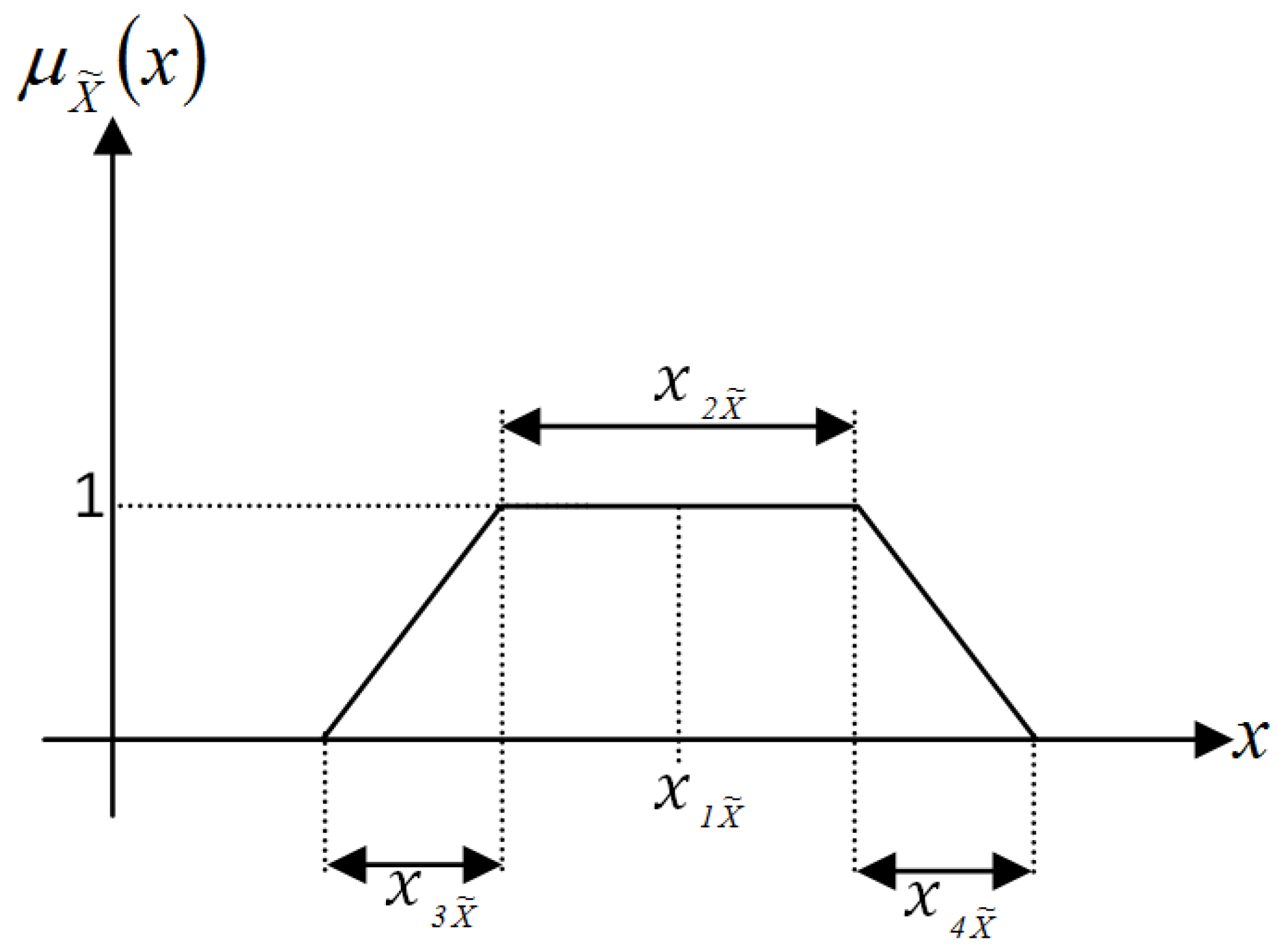
Let (TFN) $\tilde{X}$ be a trapezoidal fuzzy number. The parameterization of $\tilde{X}$ is denoted by $\tilde{X}={\left(x_{1\tilde{X}},x_{2\tilde{X}},x_{3\tilde{X}},x_{4\tilde{X}}\right)}_{TFN}$ where $x_{1\tilde{X}},x_{2\tilde{X}},x_{3\tilde{X}}$ and $x_{4\tilde{X}}$ are called the center, inner diameter, left outer radius and right outer radius respectively. The TFN $\tilde{X}$ is demonstrated in Figure 1.

Let (TAN) $\tilde{X}$ be a triangular fuzzy number. The expressed membership function for $\tilde{X}={\left(x_{\tilde{X}}^L,x_{\tilde{X}}^C,x_{\tilde{X}}^R\right)}_{TAN}$ is as follows:

$${\mu }_{\tilde{X}}\left(x\right)=\{\begin{array}{ll}0,& for x\le x^L\\ \frac{x-x_{\tilde{X}}^L}{x_{\tilde{X}}^C-x_{\tilde{X}}^L},& for x^L\le x\le x^C\\ \frac{x_{\tilde{X}}^R-x}{x_{\tilde{X}}^R-x_{\tilde{X}}^C},& for x^C\le x\le x^R\\ 0,& for x\ge x^R\end{array}$$

(8)

We will present various metrics of papers [24,25,26,27,28,29,30,31,32,33].

2.2. Various Metrics for Symbolic Numbers

Suppose ${\tilde{x}}_k$ and ${\tilde{v}}_i$ are two symbolic numbers in $p$ dimensions space, ${\tilde{x}}_k=\left\{{\tilde{x}}_{k,1},{\tilde{x}}_{k,2},\cdots ,{\tilde{x}}_{k,p}\right\},{\tilde{x}}_{k,j}={\left({\alpha }_{{\tilde{x}}_{k,j}},{\beta }_{{\tilde{x}}_{k,j}}\right)}_{SN}$ for $j=1,2,\cdots ,p$ and ${\tilde{v}}_i=\left\{{\tilde{v}}_{i,1},{\tilde{v}}_{i,2},\cdots ,{\tilde{v}}_{i,p}\right\},{\tilde{v}}_{i,j}={\left({\alpha }_{{\tilde{v}}_{i,j}},{\beta }_{{\tilde{v}}_{i,j}}\right)}_{SN}$ for $j=1,2,\cdots ,p$.

Dissimilarity defined for symbolic numbers in [24] is as follows:

$$d^2\left({\tilde{x}}_k,{\tilde{v}}_i\right)={\displaystyle \sum }_{j=1}^p\left(\begin{array}{c}{\left(1-z\right)}^2{\left({\alpha }_{{\tilde{x}}_{k,j}}-{\alpha }_{{\tilde{v}}_{i,j}}\right)}^2\\ +z^2{\left({\beta }_{{\tilde{x}}_{k,j}}-{\beta }_{{\tilde{v}}_{i,j}}\right)}^2\end{array}\right)$$

(9)

where $0\le z\le 0.5$ is center distance weight. In [25,26], dissimilarity defined for symbolic numbers can be obtained from the following equation:

$$d^2\left({\tilde{x}}_k,{\tilde{v}}_i\right)={\displaystyle \sum }_{j=1}^p{\gamma }_j\left(\begin{array}{c}{\left({\alpha }_{{\tilde{x}}_{k,j}}-{\alpha }_{{\tilde{v}}_{i,j}}\right)}^2\\ +{\left({\beta }_{{\tilde{x}}_{k,j}}-{\beta }_{{\tilde{v}}_{i,j}}\right)}^2\end{array}\right)$$

(10)

where ${\gamma }_j$ is weight vector and ${\Pi }_{j=1}^p{\gamma }_j=1$. In the section Allocation step: definition of the best partition of [25,26], dissimilarity is defined as follows:

$$d^2\left({\tilde{x}}_k,{\tilde{v}}_i\right)={\displaystyle \sum }_{j=1}^p{\gamma }_{i,j}\left(\begin{array}{c}{\left({\alpha }_{{\tilde{x}}_{k,j}}-{\alpha }_{{\tilde{v}}_{i,j}}\right)}^2\\ +{\left({\beta }_{{\tilde{x}}_{k,j}}-{\beta }_{{\tilde{v}}_{i,j}}\right)}^2\end{array}\right)$$

(11)

where ${\Pi }_{j=1}^p{\gamma }_{i,j}=1$. The last dissimilarity defined for symbolic numbers is suggested in [27] as follows:

$$d^2\left({\tilde{x}}_k,{\tilde{v}}_i\right)={\displaystyle \sum }_{j=1}^p\left(\begin{array}{c}{\left({\alpha }_{{\tilde{x}}_{k,j}}-{\alpha }_{{\tilde{v}}_{i,j}}\right)}^2\\ +{\left({\beta }_{{\tilde{x}}_{k,j}}-{\beta }_{{\tilde{v}}_{i,j}}\right)}^2\end{array}\right)$$

(12)

2.3. Various Metrics for Fuzzy Numbers

Suppose we have two LR-type fuzzy numbers ${\tilde{x}}_k$ and ${\tilde{v}}_i$ in a $p$ dimensions space, ${\tilde{x}}_k=\left\{{\tilde{x}}_{k,1},{\tilde{x}}_{k,2},\cdots ,{\tilde{x}}_{k,p}\right\}$, ${\tilde{x}}_{k,j}={\left(m_{1{\tilde{x}}_{k,j}},m_{2{\tilde{x}}_{k,j}},{\alpha }_{{\tilde{x}}_{k,j}},{\beta }_{{\tilde{x}}_{k,j}}\right)}_{LR}$ for $j=1,2,\cdots ,p$ and ${\tilde{v}}_i=\left\{{\tilde{v}}_{i,1},{\tilde{v}}_{i,2},\cdots ,{\tilde{v}}_{i,p}\right\},{\tilde{v}}_{i,j}={\left(m_{1{\tilde{v}}_{i,j}},m_{2{\tilde{v}}_{i,j}},{\alpha }_{{\tilde{v}}_{i,j}},{\beta }_{{\tilde{v}}_{i,j}}\right)}_{LR}$ for $j=1,2,\cdots ,p$. Yang et al. [29,30,32] expressed the metric $d\left({\tilde{x}}_k,{\tilde{v}}_i\right)$ with the following definition:

$$\begin{gathered} d^2\left({\tilde{x}}_k,{\tilde{v}}_i\right)={\displaystyle \sum }_{j=1}^n{d}^2\left({\tilde{x}}_{k,j},{\tilde{v}}_{i,j}\right) \\ {d}^2\left({\tilde{x}}_{k,j},{\tilde{v}}_{i,j}\right)={\left(m_{1{\tilde{x}}_{k,j}}-m_{1{\tilde{v}}_{i,j}}\right)}^2+{\left(m_{2{\tilde{x}}_{k,j}}-m_{2{\tilde{v}}_{i,j}}\right)}^2+ \\ \left(\left(m_{1{\tilde{x}}_{k,j}}-l{\alpha }_{{\tilde{x}}_{k,j}}\right)-\left(m_{1{\tilde{v}}_{i,j}}-l{\alpha }_{{\tilde{v}}_{i,j}}\right)\right){ }^2+{\left(\left(m_{2{\tilde{x}}_{k,j}}+r{\beta }_{{\tilde{x}}_{k,j}}\right)-\left(m_{2{\tilde{v}}_{i,j}}+r{\beta }_{{\tilde{v}}_{i,j}}\right)\right)}^2 \end{gathered}$$

(13)

where $l={{\displaystyle \int }}_0^1{L}^{-1}\left(w\right)dw$ and $r={{\displaystyle \int }}_0^1{R}^{-1}\left(w\right)dw$.

In the TFN numbers case, the Yang distance definition for two TFN numbers ${\tilde{x}}_k$ and ${\tilde{v}}_i$ in $p$ dimensions space, ${\tilde{x}}_k=\left\{{\tilde{x}}_{k,1},{\tilde{x}}_{k,2},\cdots ,{\tilde{x}}_{k,p}\right\}$, ${\tilde{x}}_{k,j}={\left(x_{1{\tilde{x}}_{k,j}},x_{2{\tilde{x}}_{k,j}},x_{3{\tilde{x}}_{k,j}},x_{4{\tilde{x}}_{k,j}}\right)}_{TFN}$ for $j=1,2,\cdots ,p$ and ${\tilde{v}}_i=\left\{{\tilde{v}}_{i,1},{\tilde{v}}_{i,2},\cdots ,{\tilde{v}}_{i,p}\right\}$, ${\tilde{v}}_{i,j}={\left(v_{1{\tilde{v}}_{i,j}},v_{2{\tilde{v}}_{i,j}},v_{3{\tilde{v}}_{i,j}},v_{4{\tilde{v}}_{i,j}}\right)}_{TFN}$ for $j=1,2,\cdots ,p$, is obtained from (13) by setting $l=r=\frac{1}{2}$, $m_1=\frac{2x_1-x_2}{2}$, $m_2=\frac{2x_1+x_2}{2}$, $\alpha =x_3$ and $\beta =x_4$ as follows:

$$\begin{gathered} d^2\left({\tilde{x}}_k,{\tilde{v}}_i\right)={\displaystyle \sum }_{j=1}^p{d}^2\left({\tilde{x}}_{k,j},{\tilde{v}}_{i,j}\right) \\ {d}^2\left({\tilde{x}}_{k,j},{\tilde{v}}_{i,j}\right)={\left(\frac{2x_{1{\tilde{x}}_{k,j}}-x_{2{\tilde{x}}_{k,j}}}{2}-\frac{2v_{1{\tilde{v}}_{i,j}}-v_{2{\tilde{v}}_{i,j}}}{2}\right)}^2 \\ +{\left(\begin{array}{c}\left(\frac{2x_{1{\tilde{x}}_{k,j}}-x_{2{\tilde{x}}_{k,j}}}{2}-\frac{1}{2}{x}_{3{\tilde{x}}_{k,j}}\right)-\\ \left(\frac{2v_{1{\tilde{v}}_{i,j}}-v_{2{\tilde{v}}_{i,j}}}{2}-\frac{1}{2}{v}_{3{\tilde{v}}_{i,j}}\right)\end{array}\right)}^2 \\ +{\left(\begin{array}{c}\left(\frac{2x_{1{\tilde{x}}_{k,j}}+x_{2{\tilde{x}}_{k,j}}}{2}+\frac{1}{2}{x}_{4{\tilde{x}}_{k,j}}\right)-\\ \left(\frac{2v_{1{\tilde{v}}_{i,j}}+v_{2{\tilde{v}}_{i,j}}}{2}+\frac{1}{2}{v}_{4{\tilde{v}}_{i,j}}\right)\end{array}\right)}^2 \end{gathered}$$

(14)

Dissimilarity defined for two TFN numbers ${\tilde{x}}_k,{\tilde{v}}_i$ in [28] is as follows:

$$d^2\left({\tilde{x}}_k,{\tilde{v}}_i\right)={\displaystyle \sum }_{j=1}^p\begin{array}{c}{\left(x_{1{\tilde{x}}_{k,j}}-v_{1{\tilde{v}}_{i,j}}\right)}^2+{\left(x_{2{\tilde{x}}_{k,j}}-v_{2{\tilde{v}}_{i,j}}\right)}^2\\ +{\left(x_{3{\tilde{x}}_{k,j}}-v_{3{\tilde{v}}_{i,j}}\right)}^2+{\left(x_{4{\tilde{x}}_{k,j}}-v_{4{\tilde{v}}_{i,j}}\right)}^2\end{array}$$

(15)

In the next state for LR-type fuzzy numbers suppose $m_{1{\tilde{x}}_{k,j}}=m_{2{\tilde{x}}_{k,j}}=m_{{\tilde{x}}_{k,j}}$ and $m_{1{\tilde{v}}_{i,j}}=m_{2{\tilde{v}}_{i,j}}=m_{{\tilde{v}}_{i,j}}$. The Yang distance definition for this state is as follows:

$$\begin{gathered} d^2\left({\tilde{x}}_k,{\tilde{v}}_i\right)= \\ {{\displaystyle \sum }}_{j=1}^p\left[\begin{array}{c}{\left(m_{{\tilde{x}}_{k,j}}-m_{{\tilde{v}}_{i,j}}\right)}^2\\ +{\left(\left(m_{{\tilde{x}}_{k,j}}-l{\alpha }_{{\tilde{x}}_{k,j}}\right)-\left(m_{{\tilde{v}}_{i,j}}-l{\alpha }_{{\tilde{v}}_{i,j}}\right)\right)}^2\\ +{\left(\begin{array}{c}\left(m_{{\tilde{x}}_{k,j}}+r{\beta }_{{\tilde{x}}_{k,j}}\right)\\ -\left(m_{{\tilde{v}}_{i,j}}+r{\beta }_{{\tilde{v}}_{i,j}}\right)\end{array}\right)}^2\end{array}\right] \end{gathered}$$

(16)

To achieve the robust clustering method versus noisy input numbers, Yang et al. in [31] define an exponential based metric. Dissimilarity defined for LR-type fuzzy number $\tilde{x}$ and prototype $\tilde{v}$ in [31] is as follows:

$$d^2\left({\tilde{x}}_k,{\tilde{v}}_i\right)=1-\mathit{exp}\left(-b{d}^2\left({\tilde{x}}_k,{\tilde{v}}_i\right)\right)$$

(17)

where $d^2\left({\tilde{x}}_k,{\tilde{v}}_i\right)$ is obtained from (16) and $b$ is a fixed coefficient [see [31]].

In [33] Rong et al. offer two metrics for triangular fuzzy numbers. Dissimilarity defined for triangular-type fuzzy numbers ${\tilde{x}}_k$ and ${\tilde{v}}_i$ in $p$ dimensions space, ${\tilde{x}}_k=\left\{{\tilde{x}}_{k,1},{\tilde{x}}_{k,2},\cdots ,{\tilde{x}}_{k,p}\right\},{\tilde{x}}_{k,j}={\left(x_{k,j}^L,x_{k,j}^C,x_{k,j}^R\right)}_{TAN}$ for $j=1,2,\cdots ,p$ and ${\tilde{v}}_i=\left\{{\tilde{v}}_{i,1},{\tilde{v}}_{i,2},\cdots ,{\tilde{v}}_{i,p}\right\},v_{i,j}={\left(v_{i,j}^L,v_{i,j}^C,v_{i,j}^R\right)}_{TAN}$ for $j=1,2,\cdots ,p$, is as follows:

$$\begin{array}{l}{d}^2\left({\tilde{x}}_{k,j},{\tilde{v}}_{i,j}\right)=\frac{{\alpha }_1}{6}{(x_{k,j}^L-v_{i,j}^L)}^2+\left(\frac{{\alpha }_1}{6}+{\alpha }_2+\frac{{\alpha }_3}{6}\right){(x_{k,j}^C-v_i^C)}^2+\frac{{\alpha }_3}{6}{(x_{k,j}^R-v_{i,j}^R)}^2\\ +\frac{{\alpha }_1}{6}{\left((x_{k,j}^L+x_{k,j}^C)-(v_{i,j}^L+v_{i,j}^C)\right)}^2+\frac{{\alpha }_3}{6}{\left((x_{k,j}^R+x_{k,j}^C)-(v_{i,j}^R+v_{i,j}^C)\right)}^2\\ d_1^2\left({\tilde{x}}_k,{\tilde{v}}_i\right)={\displaystyle {\displaystyle \sum }_{j=1}^p}{d}^2\left({\tilde{x}}_{k,j},{\tilde{v}}_{i,j}\right)\left(18-1\right)\\ d_2^2\left({\tilde{x}}_k,{\tilde{v}}_i\right)=1-\mathit{exp}\left(-b.d_1^2\left({\tilde{x}}_k,{\tilde{v}}_i\right)\right)\left(18-2\right)\end{array}$$

(18)

where ${\alpha }_1$,${\alpha }_2$ and ${\alpha }_3$ are positive, fixed and known coefficients while ${\alpha }_1+{\alpha }_2+{\alpha }_3=1$ and b is a fixed coefficient also.

The main key point in the proposed Vector Fuzzy c-Spherical Shells (VFCSS) Clustering is how to define crisp vectors from parameters of affected numbers. According to any used metric, we define a crisp vectors set $Y=\left\{y_1,y_2,\cdots ,y_n\right\}$ a corresponding input numbers set ($\tilde{X}$ for non-crisp numbers and $X$ for crisp numbers) and $W=\left\{w_1,w_2,\cdots ,w_c\right\}$ and a corresponding centers set ($\tilde{V}$ for non-crisp numbers and $V$ for crisp numbers). These definitions allow us to demonstrate a distance and a Lagrange function in the proposed VFCSS as follows:

$$d^2={\left(\Vert y_k-w_i\Vert {}^2-r_i{}^2\right)}^2={({\left(y_k-w_i\right)}^T\left(y_k-w_i\right)-r_i{}^2)}^2$$

(19)

$$L\left(W,U,\lambda \right)={\displaystyle \sum }_{k=1}^n{\displaystyle \sum }_{i=1}^c{u}_{i,k}^m{({\left(y_k-w_i\right)}^T\left(y_k-w_i\right)-r_i{}^2)}^2+{\displaystyle \sum }_{k=1}^n{\lambda }_k\left({\displaystyle \sum }_{i=1}^c{u}_{i,k}-1\right)$$

(20)

By this definition, similar to the crisp case and (5), the membership value of $u_{i,k}$ can update from the next equation in the proposed VFCSS:

$$\begin{gathered} u_{i,k}={\left({\displaystyle \sum }_{j=1}^c{\left(\frac{d^2\left(y_k,w_i,r_i\right)}{d^2\left(y_k,w_j,r_j\right)}\right)}^{\frac{1}{m-1}}\right)}^{-1} \\ ={\left({\displaystyle \sum }_{j=1}^c{\left(\frac{({\left(y_k-w_i\right)}^T\left(y_k-w_i\right)-r_i{}^2)}{({\left(y_k-w_j\right)}^T\left(y_k-w_j\right)-r_j{}^2)}\right)}^{\frac{2}{m-1}}\right)}^{-1} \end{gathered}$$

(21)

Let the independent parameters of the $i$th center (except radius $r_i$) be denoted by the set $\left\{t_i\right\}$. After creating the Lagrange function (20), we must calculate the derivation of the Lagrange function with respect to parameters $t_i,r_i$ and set the resulting equation equal to zero for all $t_i$’s as follows:

$$\begin{array}{l}\raisebox{1ex}{$\partial L$}\!\left/ \!\raisebox{-1ex}{$\partial t_i$}\right.=\raisebox{1ex}{$\partial L$}\!\left/ \!\raisebox{-1ex}{$\partial w_i$}\right..\raisebox{1ex}{$\partial w_i^T$}\!\left/ \!\raisebox{-1ex}{$\partial t_i$}\right.=0,for all t_i\\ \raisebox{1ex}{$\partial L$}\!\left/ \!\raisebox{-1ex}{$\partial r_i$}\right.=\raisebox{1ex}{$\partial L$}\!\left/ \!\raisebox{-1ex}{$\partial w_i$}\right..\raisebox{1ex}{$\partial w_i^T$}\!\left/ \!\raisebox{-1ex}{$\partial r_i$}\right.=0\end{array}\} for i=1,2,\cdots ,c$$

(22)

As $t_i$s are independent and we have $\raisebox{1ex}{$\partial L$}\!\left/ \!\raisebox{-1ex}{$\partial w_i$}\right..\raisebox{1ex}{$\partial w_i^T$}\!\left/ \!\raisebox{-1ex}{$\partial t_i$}\right.=0$ for all $t_i$s, furthermore $\raisebox{1ex}{$\partial L$}\!\left/ \!\raisebox{-1ex}{$\partial w_i$}\right.$ is fixed while $\raisebox{1ex}{$\partial w_i^T$}\!\left/ \!\raisebox{-1ex}{$\partial t_i$}\right.$ is changing because of changing the metric (in fixed $t_i$), therefore from (22) we can conclude that $\raisebox{1ex}{$\partial L$}\!\left/ \!\raisebox{-1ex}{$\partial w_i$}\right.=0$. Suppose the vectors ${\left\{w_i\right\}}_{i=1}^c$ and ${\left\{y_k\right\}}_{k=1}^n$ are $\widehat{p}$-dimensional, then we can extract the updating relation of $w_i$ and $r_i$ similar to $v_i$ and $r_i$ in the crisp numbers case as follows:

$$\{\begin{array}{l}{w}_i=-\frac{1}{2}{[q_{i,1},q_{i,2},\cdots ,q_{i,\widehat{p}}]}^T\\ r_i=\sqrt{w_i^T{w}_i-q_{i,\widehat{p}+1}}\end{array}, for i=1,2,\cdots ,c$$

(23a)

$$Where:\{\begin{array}{ll}{q}_i=-\frac{1}{2}{H}_i^{-1}{\omega }_i& \left(23\mathrm{b}\right)\\ H_i={\displaystyle {\displaystyle \sum }_{k=1}^n}{u}_{i,k}^m{g}_k{g}_k^T& \left(23\mathrm{c}\right)\\ {\omega }_i={\displaystyle {\displaystyle \sum }_{k=1}^n}{u}_{i,k}^m{s}_k& \left(23\mathrm{d}\right)\\ s_k=2\left(y_k^T{y}_k\right)g_k, for k=1,2,\cdots ,n& \left(23\mathrm{e}\right)\\ g_k={\left[y_{k,1},y_{k,2},\cdots ,y_{k,\widehat{p}},1\right]}^T, for k=1,2,\cdots ,n& \left(23\mathrm{f}\right)\end{array}$$

Subsequently by multiplying both sides of the first phrase of (23a) ($w_i=-\frac{1}{2}{\left[q_{i,1},q_{i,2},\cdots ,q_{i,\widehat{p}}\right]}^T$) by $\raisebox{1ex}{$\partial w_i^T$}\!\left/ \!\raisebox{-1ex}{$\partial t_i$}\right.$, we can get the updating equation of the $t_i$ parameter. For simplicity, we replace $\raisebox{1ex}{$\partial w_i^T$}\!\left/ \!\raisebox{-1ex}{$\partial t_i$}\right.$ by ${\xi }_{t_i}$, that is the normalized vector of the $\raisebox{1ex}{$\partial w_i^T$}\!\left/ \!\raisebox{-1ex}{$\partial t_i$}\right.$ vector. Therefore, the updated relation for the $t_i$ parameter can be obtained as follows:

$${\xi }_{t_i}=Norm\left(\raisebox{1ex}{$\partial w_i^T$}\!\left/ \!\raisebox{-1ex}{$\partial t_i$}\right.\right), for all t_{i}s and i=1,2,\cdots ,c$$

(24)

$${\xi }_{t_i}{w}_i=-\frac{1}{2}{\xi }_{t_i}{\left[q_{i,1},q_{i,2},\cdots ,q_{i,\widehat{p}}\right]}^T\Rightarrow t_i=?,for all t_{i}s and i=1,2,\cdots ,c.$$

(25)

To complete the VFCSS description, we will apply the proposed VFCSS clustering method over various crisp and non-crisp numbers.

In this part, we apply the proposed VFCSS clustering of Section 4 over crisp and various non-crisp numbers with the metrics that are introduced in Section 3.

2.4. VFCSS Applied to Crisp Numbers

The VFCSS can be applied over crisp numbers. In this state according to the definition of Euclidean distance, the definition of the $Y$ and $W$ sets are as follows:

$$\begin{gathered} Y=\left\{y_1,y_2,\cdots ,y_n\right\},y_k={\left[y_{k,1},y_{k,2},\cdots ,y_{k,p}\right]}^T,y_{k,j}=x_{k,j} \\ W=\left\{w_1,w_2,\cdots ,w_c\right\},w_i={\left[w_{i,1},w_{i,2},\cdots ,w_{i,p}\right]}^T,w_{i,j}=v_{i,j} \end{gathered}$$

(26)

where $k=1,2,\cdots ,n$, $i=1,2,\cdots ,c$ and $j=1,2,\cdots ,p$. In this case $Y=X$ and $W=V$. Therefore, we can conclude $\widehat{p}=p$. In this case ${\xi }_{t_i}=Norm\left(\raisebox{1ex}{$\partial w_i^T$}\!\left/ \!\raisebox{-1ex}{$\partial t_i$}\right.\right)=\raisebox{1ex}{$\partial w_i^T$}\!\left/ \!\raisebox{-1ex}{$\partial t_i$}\right.$ that is obtained from

Table 1. $\xi$ for VFCSS applying over crisp numbers.

d$t_i$	$v_{i,j},for j=1,2,\cdots ,p$
${\xi }_{t_i}=Norm\left(\raisebox{1ex}{$\partial w_i^T$}\!\left/ \!\raisebox{-1ex}{$\partial t_i$}\right.\right)=\raisebox{1ex}{$\partial w_i^T$}\!\left/ \!\raisebox{-1ex}{$\partial t_i$}\right.$	$\left[\stackrel{\left(j-1\right)}{\overbrace{0,0,\cdots ,0}},1,\stackrel{\left(p-j\right)}{\overbrace{0,0,\cdots ,0}}\right]$

.

Then using (25), parameter $t_i$ can be obtained as (5). We can conclude the VFCSS applied over crisp numbers is equivalent with this concept in the first Equation of (5a).

2.5. The VFCSS Applied to Fuzzy Numbers

In this part, we apply VFCSS clustering to various introduced fuzzy type numbers, see Section 3.

2.5.1. The VFCSS Applied to LR-Type Fuzzy Numbers

For LR-type fuzzy numbers, when the metric (13) is used, we define Y and $W$ sets as below:

$$\begin{gathered} Y=\left\{y_1,y_2,\cdots ,y_n\right\},y_k={\left[y_{k,1},y_{k,2},\cdots ,y_{k,p}\right]}^T,y_{k,j} \\ ={\left[m_{1{\tilde{x}}_{k,j}},m_{2{\tilde{x}}_{k,j}},m_{1{\tilde{x}}_{k,j}}-l{\alpha }_{{\tilde{x}}_{k,j}},m_{2{\tilde{x}}_{k,j}}+r{\beta }_{{\tilde{x}}_{k,j}}\right]}^T \\ W=\left\{w_1,w_2,\cdots ,w_c\right\},w_i={\left[w_{i,1},w_{i,2},\cdots ,w_{i,p}\right]}^T,w_{i,j} \\ ={\left[m_{1{\tilde{v}}_{i,j}},m_{2{\tilde{v}}_{i,j}},m_{1{\tilde{v}}_{i,j}}-l{\alpha }_{{\tilde{v}}_{i,j}},m_{2{\tilde{v}}_{i,j}}+r{\beta }_{{\tilde{v}}_{i,j}}\right]}^T \end{gathered}$$

(27)

where $k=1,2,\cdots ,n$, $i=1,2,\cdots ,c$ and $j=1,2,\cdots ,p$. It is observed in this case $\widehat{p}=4p$. In this case, for all $t_i$s ($t_i\in {\left\{m_{1{\tilde{v}}_{i,j}},m_{2{\tilde{v}}_{i,j}},{\alpha }_{{\tilde{v}}_{i,j}},{\beta }_{{\tilde{v}}_{i,j}}\right\}}_{j=1}^p$), $\raisebox{1ex}{$\partial w_i^T$}\!\left/ \!\raisebox{-1ex}{$\partial t_i$}\right.$ and ${\xi }_{t_i}$ are obtained in

Table 2. $\raisebox{1ex}{$ \partial w^T$}\!\left/ \!\raisebox{-1ex}{$\partial t$}\right.$ for VFCSS applying over LR-type fuzzy numbers when metric (13) is used.

$t_i$	$m_{1{\tilde{v}}_{i,j}},for j=1,2,\cdots ,p$	$m_{2{\tilde{v}}_{i,j}},for j=1,2,\cdots ,p$	${\alpha }_{{\tilde{v}}_{i,j}},for j=1,2,\cdots ,p$	${\beta }_{{\tilde{v}}_{i,j}},for j=1,2,\cdots ,p$
$\raisebox{1ex}{$\partial w_i^T$}\!\left/ \!\raisebox{-1ex}{$\partial t_i$}\right.$	$\left[\stackrel{4\left(j-1\right)}{\overbrace{0,0,\cdots ,0}},1,0,1,0,\stackrel{4\left(p-j\right)}{\overbrace{0,0,\cdots ,0}}\right]$	$\left[\stackrel{4\left(j-1\right)}{\overbrace{0,0,\cdots ,0}},0,1,0,1,\stackrel{4\left(p-j\right)}{\overbrace{0,0,\cdots ,0}}\right]$	$\left[\stackrel{4\left(j-1\right)+2}{\overbrace{0,0,\cdots ,0}},-l,\stackrel{4\left(p-j\right)+1}{\overbrace{0,0,\cdots ,0}}\right]$	$\left[\stackrel{4\left(j-1\right)+3}{\overbrace{0,0,\cdots ,0}},r,\stackrel{4\left(p-j\right)}{\overbrace{0,0,\cdots ,0}}\right]$

and

Table 3. $\xi$ for VFCSS applying over LR-type fuzzy numbers when metric (13) is used.

$t_i$	$m_{1{\tilde{v}}_{i,j}},for j=1,2,\cdots ,p$	$m_{2{\tilde{v}}_{i,j}},for j=1,2,\cdots ,p$	${\alpha }_{{\tilde{v}}_{i,j}},for j=1,2,\cdots ,p$	${\beta }_{{\tilde{v}}_{i,j}},for j=1,2,\cdots ,p$
${\xi }_{t_i}$	$\left[\stackrel{4\left(j-1\right)}{\overbrace{0,0,\cdots ,0}},1,0,1,0,\stackrel{4\left(p-j\right)}{\overbrace{0,0,\cdots ,0}}\right]$	$\left[\stackrel{4\left(j-1\right)}{\overbrace{0,0,\cdots ,0}},0,1,0,1,\stackrel{4\left(p-j\right)}{\overbrace{0,0,\cdots ,0}}\right]$	$\left[\stackrel{4\left(j-1\right)+2}{\overbrace{0,0,\cdots ,0}},1,\stackrel{4\left(p-j\right)+1}{\overbrace{0,0,\cdots ,0}}\right]$	$\left[\stackrel{4\left(j-1\right)+3}{\overbrace{0,0,\cdots ,0}},1,\stackrel{4\left(p-j\right)}{\overbrace{0,0,\cdots ,0}}\right]$

.

Finally, we can arrive at updated relations of parameters $m_{1{\tilde{v}}_{i,j}},m_{2{\tilde{v}}_{i,j}},{\alpha }_{{\tilde{v}}_{i,j}}$ and ${\beta }_{{\tilde{v}}_{i,j}}$ from (25) as follows:

$$\begin{array}{l}{m}_{1{\tilde{v}}_{i,j}}=-\frac{1}{4}\left(q_{i,4j-3}+q_{i,4j-1}\right)+\frac{l}{2}{\alpha }_{{\tilde{v}}_{i,j}}\\ m_{2{\tilde{v}}_{i,j}}=-\frac{1}{4}\left(q_{i,4j-2}+q_{i,4j}\right)-\frac{r}{2}{\beta }_{{\tilde{v}}_{i,j}}\\ {\alpha }_{{\tilde{v}}_{i,j}}=\frac{1}{2l}{q}_{i,4j-1}+\frac{1}{l}{m}_{1{\tilde{v}}_{i,j}}\\ {\beta }_{{\tilde{v}}_{i,j}}=-\frac{1}{2r}{q}_{i,4j}-\frac{1}{r}{m}_{2{\tilde{v}}_{i,j}}\end{array}\}for\{\begin{array}{c}i=1,2,\cdots ,c\\ j=1,2,\cdots ,p\end{array}$$

(28)

In the other state of LR-type fuzzy numbers, suppose $m_{1{\tilde{x}}_{k,j}}=m_{2{\tilde{x}}_{k,j}}=m_{{\tilde{x}}_{k,j}}$ and $m_{1{\tilde{v}}_{i,j}}=m_{2{\tilde{v}}_{i,j}}=m_{{\tilde{v}}_{i,j}}$. Regarding the Yang distance definition of (16), $Y$ and $W$ are defined as follows:

$$\begin{gathered} Y=\left\{y_1,y_2,\cdots ,y_n\right\},y_k={\left[y_{k,1},y_{k,2},\cdots ,y_{k,p}\right]}^T, \\ {y}_{k,j}={\left[m_{{\tilde{x}}_{k,j}},m_{{\tilde{x}}_{k,j}}-l{\alpha }_{{\tilde{x}}_{k,j}},m_{{\tilde{x}}_{k,j}}+r{\beta }_{{\tilde{x}}_{k,j}}\right]}^T \\ W=\left\{w_1,w_2,\cdots ,w_c\right\},w_i={\left[w_{i,1},w_{i,2},\cdots ,w_{i,p}\right]}^T, \\ {w}_{i,j}={\left[m_{{\tilde{v}}_{i,j}},m_{{\tilde{v}}_{i,j}}-l{\alpha }_{{\tilde{v}}_{i,j}},m_{{\tilde{v}}_{i,j}}+r{\beta }_{{\tilde{v}}_{i,j}}\right]}^T \end{gathered}$$

(29)

In this case $\widehat{p}=3p$. For this case ${\xi }_{t_i}$ and updated relations of $m_{{\tilde{v}}_{i,j}},{\alpha }_{{\tilde{v}}_{i,j}}$ and ${\beta }_{{\tilde{v}}_{i,j}}$ are as in

Table 4. ξ for VFCSS applying over LR-type fuzzy numbers when metric (16) is used.

$t_i$	$m_{{\tilde{v}}_{i,j}},for j=1,2,\cdots ,p$	${\alpha }_{{\tilde{v}}_{i,j}},for j=1,2,\cdots ,p$	${\beta }_{{\tilde{v}}_{i,j}},for j=1,2,\cdots ,p$
${\xi }_{t_i}$	$\left[\stackrel{3\left(j-1\right)}{\overbrace{0,0,\cdots ,0}},1,1,1,\stackrel{3\left(p-j\right)}{\overbrace{0,0,\cdots ,0}}\right]$	$\left[\stackrel{3\left(j-1\right)+1}{\overbrace{0,0,\cdots ,0}},1,\stackrel{3\left(p-j\right)+1}{\overbrace{0,0,\cdots ,0}}\right]$	$\left[\stackrel{3\left(j-1\right)+2}{\overbrace{0,0,\cdots ,0}},1,\stackrel{3\left(p-j\right)}{\overbrace{0,0,\cdots ,0}}\right]$

and (30).

$$\begin{array}{l}{m}_{{\tilde{v}}_{i,j}}=-\frac{1}{6}\left(q_{i,3j-2}+q_{i,3j-1}+q_{i,3j}\right)+\frac{l}{3}{\alpha }_{{\tilde{v}}_{i,j}}-\frac{r}{3}{\beta }_{{\tilde{v}}_{i,j}}\\ {\alpha }_{{\tilde{v}}_{i,j}}=\frac{1}{2l}{q}_{i,3j-1}+\frac{1}{l}{m}_{{\tilde{v}}_{i,j}}\\ {\beta }_{{\tilde{v}}_{i,j}}=-\frac{1}{2r}{q}_{i,3j}-\frac{1}{r}{m}_{{\tilde{v}}_{i,j}}\end{array}\}for\{\begin{array}{c}i=1,2,\cdots ,c\\ j=1,2,\cdots ,p\end{array}$$

(30)

As we cannot define Y and W to match (17) to (19), therefore the proposed VFCSS cannot be applied on (19).

2.5.2. The VFCSS Applied to TFN-Type Fuzzy Numbers

For TFN numbers, when the metric (14) is used, we define Y and $W$ sets as below:

$$\begin{array}{ll}Y=\left\{y_1,y_2,\cdots ,y_n\right\},y_k& ={\left[y_{k,1},y_{k,2},\cdots ,y_{k,p}\right]}^T,y_{k,j}\\ & ={\left[\frac{2x_{1{\tilde{x}}_{k,j}}-x_{2{\tilde{x}}_{k,j}}}{2},\frac{2x_{1{\tilde{x}}_{k,j}}+x_{2{\tilde{x}}_{k,j}}}{2},\frac{2x_{1{\tilde{x}}_{k,j}}-x_{2{\tilde{x}}_{k,j}}-x_{3{\tilde{x}}_{k,j}}}{2},\frac{2x_{1{\tilde{x}}_{k,j}}+x_{2{\tilde{x}}_{k,j}}+x_{4{\tilde{x}}_{k,j}}}{2}\right]}^T\\ W=\left\{w_1,w_2,\cdots ,w_c\right\},w_i& ={\left[w_{i,1},w_{i,2},\cdots ,w_{i,p}\right]}^T,w_{i,j}\\ & ={\left[\frac{2v_{1{\tilde{v}}_{i,j}}-v_{2{\tilde{v}}_{i,j}}}{2},\frac{2v_{1{\tilde{v}}_{i,j}}+v_{2{\tilde{v}}_{i,j}}}{2},\frac{2v_{1{\tilde{v}}_{i,j}}-v_{2{\tilde{v}}_{i,j}}-v_{3{\tilde{v}}_{i,j}}}{2},\frac{2v_{1{\tilde{v}}_{i,j}}+v_{2{\tilde{v}}_{i,j}}+v_{4{\tilde{v}}_{i,j}}}{2}\right]}^T\end{array}$$

(31)

It is observed $\widehat{p}=4p$. In this case ${\xi }_{t_i}$ and updated relations of $v_{1{\tilde{v}}_{i,j}},v_{2{\tilde{v}}_{i,j}},v_{3{\tilde{v}}_{i,j}}$ and $v_{4{\tilde{v}}_{i,j}}$ are as in

Table 5. $\xi$ for VFCSS applying over TFN-type fuzzy numbers when metric (14) is used.

$t_i$	$v_{1{\tilde{v}}_{i,j}},for j=1,2,\cdots ,p$	$v_{2{\tilde{v}}_{i,j}},for j=1,2,\cdots ,p$	$v_{3{\tilde{v}}_{i,j}},for j=1,2,\cdots ,p$	$v_{4{\tilde{v}}_{i,j}},for j=1,2,\cdots ,p$
${\xi }_{t_i}$	$\left[\stackrel{4\left(j-1\right)}{\overbrace{0,0,\cdots ,0}},1,1,1,1,\stackrel{4\left(p-j\right)}{\overbrace{0,0,\cdots ,0}}\right]$	$\left[\stackrel{4\left(j-1\right)}{\overbrace{0,0,\cdots ,0}},-1,1,-1,1,\stackrel{4\left(p-j\right)}{\overbrace{0,0,\cdots ,0}}\right]$	$\left[\stackrel{4\left(j-1\right)+2}{\overbrace{0,0,\cdots ,0}},1,\stackrel{4\left(p-j\right)+1}{\overbrace{0,0,\cdots ,0}}\right]$	$\left[\stackrel{4\left(j-1\right)+3}{\overbrace{0,0,\cdots ,0}},1,\stackrel{4\left(p-j\right)}{\overbrace{0,0,\cdots ,0}}\right]$

and (32).

$$\begin{array}{l}{v}_{1{\tilde{v}}_{i,j}}=-\frac{1}{8}\left(q_{i,4j-3}+q_{i,4j-2}+q_{i,4j-1}+q_{i,4j}-v_{3{\tilde{v}}_{i,j}}+v_{4{\tilde{v}}_{i,j}}\right)\\ v_{2{\tilde{v}}_{i,j}}=-\frac{1}{4}\left(-q_{i,4j-3}+q_{i,4j-2}-q_{i,4j-1}+q_{i,4j}+v_{3{\tilde{v}}_{i,j}}+v_{4{\tilde{v}}_{i,j}}\right)\\ v_{3{\tilde{v}}_{i,j}}=q_{i,4j-1}+2v_{1{\tilde{v}}_{i,j}}-v_{2{\tilde{v}}_{i,j}}\\ v_{4{\tilde{v}}_{i,j}}=-q_{i,4j}-2v_{1{\tilde{v}}_{i,j}}-v_{2{\tilde{v}}_{i,j}}\end{array}\}for\{\begin{array}{c}i=1,2,\cdots ,c\\ j=1,2,\cdots ,p\end{array}$$

(32)

For TFN numbers when metric (15) is used, we define the Y and $W$ sets as follows:

$$\begin{gathered} Y=\left\{y_1,y_2,\cdots ,y_n\right\},y_k={\left[y_{k,1},y_{k,2},\cdots ,y_{k,p}\right]}^T,y_{k,j}={\left[x_{1{\tilde{x}}_{k,j}},x_{2{\tilde{x}}_{k,j}},x_{3{\tilde{x}}_{k,j}},x_{4{\tilde{x}}_{k,j}}\right]}^T \\ W=\left\{w_1,w_2,\cdots ,w_c\right\},w_i={\left[w_{i,1},w_{i,2},\cdots ,w_{i,p}\right]}^T,w_{i,j}={\left[v_{1{\tilde{v}}_{i,j}},v_{2{\tilde{v}}_{i,j}},v_{3{\tilde{v}}_{i,j}},v_{4{\tilde{v}}_{i,j}}\right]}^T \end{gathered}$$

(33)

In this case $\widehat{p}=4p$, furthermore ${\xi }_{t_i}$ and updated relations of $v_{1{\tilde{v}}_{i,j}},v_{2{\tilde{v}}_{i,j}},v_{3{\tilde{v}}_{i,j}}$ and $v_{4{\tilde{v}}_{i,j}}$ are as in

Table 6. $\xi$ for VFCSS over applying over TFN-type fuzzy numbers when metric (14) is used.

$t_i$	$v_{1{\tilde{v}}_{i,j}},for j=1,2,\cdots ,p$	$v_{2{\tilde{v}}_{i,j}},for j=1,2,\cdots ,p$	$v_{3{\tilde{v}}_{i,j}},for j=1,2,\cdots ,p$	$v_{4{\tilde{v}}_{i,j}},for j=1,2,\cdots ,p$
${\xi }_{t_i}$	$\left[\stackrel{4\left(j-1\right)}{\overbrace{0,0,\cdots ,0}},1,\stackrel{4\left(p-j\right)+3}{\overbrace{0,0,\cdots ,0}}\right]$	$\left[\stackrel{4\left(j-1\right)+1}{\overbrace{0,0,\cdots ,0}},1,\stackrel{4\left(p-j\right)+2}{\overbrace{0,0,\cdots ,0}}\right]$	$\left[\stackrel{4\left(j-1\right)+2}{\overbrace{0,0,\cdots ,0}},1,\stackrel{4\left(p-j\right)+1}{\overbrace{0,0,\cdots ,0}}\right]$	$\left[\stackrel{4\left(j-1\right)+3}{\overbrace{0,0,\cdots ,0}},1,\stackrel{4\left(p-j\right)}{\overbrace{0,0,\cdots ,0}}\right]$

and (34).

$$\begin{array}{l}{v}_{1{\tilde{v}}_{i,j}}=-\frac{1}{2}{q}_{i,4j-3}\\ v_{2{\tilde{v}}_{i,j}}=-\frac{1}{2}{q}_{i,4j-2}\\ v_{3{\tilde{v}}_{i,j}}=-\frac{1}{2}{q}_{i,4j-1}\\ v_{4{\tilde{v}}_{i,j}}=-\frac{1}{2}{q}_{i,4j}\end{array}\}for\{\begin{array}{c}i=1,2,\cdots ,c\\ j=1,2,\cdots ,p\end{array}$$

(34)

2.5.3. The VFCSS Applied to TAN-Type Fuzzy Numbers

If we use (18.1) as the metric when we apply VFCSS over TAN numbers, the definition of Y and $W$ is as follows:

$$\begin{gathered} Y=\left\{y_1,y_2,\cdots ,y_n\right\},y_k={\left[y_{k,1},y_{k,2},\cdots ,y_{k,p}\right]}^T,y_{k,j}={\left[\sqrt{\frac{{\alpha }_1}{6}}{x}_{k,j}^L,\sqrt{\frac{{\alpha }_1}{6}+{\alpha }_2+\frac{{\alpha }_3}{6}}{x}_{k,j}^C,\sqrt{\frac{{\alpha }_3}{6}}{x}_{k,j}^R,\sqrt{\frac{{\alpha }_1}{6}}\left(x_{k,j}^L+x_{k,j}^C\right),\sqrt{\frac{{\alpha }_3}{6}}\left(x_{k,j}^R+x_{k,j}^C\right)\right]}^T \\ W=\left\{w_1,w_2,\cdots ,w_c\right\},w_i={\left[w_{i,1},w_{i,2},\cdots ,w_{i,p}\right]}^T,w_{i,j}={\left[\sqrt{\frac{{\alpha }_1}{6}}{v}_{i,j}^L,\sqrt{\frac{{\alpha }_1}{6}+{\alpha }_2+\frac{{\alpha }_3}{6}}{v}_{i,j}^C,\sqrt{\frac{{\alpha }_3}{6}}{v}_{i,j}^R,\sqrt{\frac{{\alpha }_1}{6}}\left(v_{i,j}^L+v_{i,j}^C\right),\sqrt{\frac{{\alpha }_3}{6}}\left(v_{i,j}^R+v_{i,j}^C\right)\right]}^T \end{gathered}$$

(35)

In this case $\widehat{p}=5p$, furthermore ${\xi }_{t_i}$ and updated relations of $v_{i,j}^L,v_{i,j}^C$ and $v_{i,j}^R$ are as in

Table 7. $\xi$ for VFCSS applying over TAN-type fuzzy numbers when metric (18.1) is used.

$t_i$	$v_{i,j}^L,for j=1,2,\cdots ,p$	$v_{i,j}^C,for j=1,2,\cdots ,p$	$v_{i,j}^R,for j=1,2,\cdots ,p$
${\xi }_{t_i}$	$\left[\stackrel{5\left(j-1\right)}{\overbrace{0,0,\cdots ,0}},1,00,1,0,\stackrel{5\left(p-j\right)}{\overbrace{0,0,\cdots ,0}}\right]$	$\left[\stackrel{5\left(j-1\right)}{\overbrace{0,0,\cdots ,0}},0,1,0,\sqrt{\frac{{\alpha }_1}{{\alpha }_1+6{\alpha }_2+{\alpha }_3}},\sqrt{\frac{{\alpha }_3}{{\alpha }_1+6{\alpha }_2+{\alpha }_3}},\stackrel{5\left(p-j\right)}{\overbrace{0,0,\cdots ,0}}\right]$	$\left[\stackrel{5\left(j-1\right)}{\overbrace{0,0,\cdots ,0}},0,0,1,0,1,\stackrel{5\left(p-j\right)}{\overbrace{0,0,\cdots ,0}}\right]$

and (36).

$$\begin{array}{l}{v}_{i,j}^L=-\sqrt{\frac{3}{8{\alpha }_1}}\left(q_{i,5j-4}+q_{i,5j-1}\right)-\frac{1}{2}{v}_{i,j}^C\\ v_{i,j}^C=-\frac{\sqrt{6}}{4\left({\alpha }_1+3{\alpha }_2+{\alpha }_3\right)}\left(\sqrt{\left({\alpha }_1+6{\alpha }_2+{\alpha }_3\right)}{q}_{i,5j-3}+\sqrt{{\alpha }_1}{q}_{i,5j-1}+\sqrt{{\alpha }_3}{q}_{i,5j}\right)-\frac{{\alpha }_1{v}_{i,j}^L+{\alpha }_3{v}_{i,j}^R}{2\left({\alpha }_1+3{\alpha }_2+{\alpha }_3\right)}\\ v_{i,j}^R=-\sqrt{\frac{3}{8{\alpha }_1}}\left(q_{i,5j-2}+q_{i,5j}\right)-\frac{1}{2}{v}_{i,j}^C\end{array}\}$$

(36)

However, the proposed VFCSS cannot be implemented for the exponential based metric of (18.1).

2.6. The VFCSS over Symbolic Numbers

Using the VFCSS method, the definition of the $Y$ and $W$ crisp vectors for dissimilarity definitions of (12) is as follows:

$$\begin{gathered} Y=\left\{y_1,y_2,\cdots ,y_n\right\},y_k={\left[y_{k,1},y_{k,2},\cdots ,y_{k,p}\right]}^T, y_{k,j}={\left[{\alpha }_{{\tilde{x}}_{k,j}},{\beta }_{{\tilde{x}}_{k,j}}\right]}^T \\ W=\left\{w_1,w_2,\cdots ,w_c\right\},w_i={\left[w_{i,1},w_{i,2},\cdots ,w_{i,p}\right]}^T, w_{i,j}={\left[{\alpha }_{{\tilde{v}}_{i,j}},{\beta }_{{\tilde{v}}_{i,j}}\right]}^T \end{gathered}$$

(37)

In this case $\widehat{p}=2p$. For this case ${\xi }_{t_i}$ and updated relations of ${\alpha }_{{\tilde{v}}_{i,j}}$ and ${\beta }_{{\tilde{v}}_{i,j}}$ are as in

Table 8. $\xi$ for VFCSS applying over symbolic numbers when metric (12) is used.

$t_i$	${\alpha }_{{\tilde{v}}_{i,j}},for j=1,2,\cdots ,p$	${\beta }_{{\tilde{v}}_{i,j}},for j=1,2,\cdots ,p$
${\xi }_{t_i}$	$\left[\stackrel{2\left(j-1\right)}{\overbrace{0,0,\cdots ,0}},1,\stackrel{2\left(p-j\right)+1}{\overbrace{0,0,\cdots ,0}}\right]$	$\left[\stackrel{2\left(j-1\right)+1}{\overbrace{0,0,\cdots ,0}},1,\stackrel{2\left(p-j\right)}{\overbrace{0,0,\cdots ,0}}\right]$

and Equation (38).

$$\begin{array}{l}{\alpha }_{{\tilde{v}}_{i,j}}=-\frac{1}{2}{q}_{i,2j-1}\\ {\beta }_{{\tilde{v}}_{i,j}}=-\frac{1}{2}{q}_{i,2j}\end{array}\}for \{\begin{array}{c}i=1,2,\cdots ,c\\ j=1,2,\cdots ,p\end{array}$$

(38)

Using the VFCSS method, the definition of the $Y$ and $W$ vectors for metric (9) is as follows:

$$\begin{gathered} Y=\left\{y_1,y_2,\cdots ,y_n\right\},y_k={\left[y_{k,1},y_{k,2},\cdots ,y_{k,p}\right]}^T,y_{k,j}={\left[\left(1-z\right){\alpha }_{{\tilde{x}}_{k,j}},z{\beta }_{{\tilde{x}}_{k,j}}\right]}^T \\ W=\left\{w_1,w_2,\cdots ,w_c\right\},w_i={\left[w_{i,1},w_{i,2},\cdots ,w_{i,p}\right]}^T,w_{i,j}={\left[\left(1-z\right){\alpha }_{{\tilde{v}}_{i,j}},z{\beta }_{{\tilde{v}}_{i,j}}\right]}^T \end{gathered}$$

(39)

Using these definitions, dissimilarity between two symbolic numbers ${\tilde{x}}_k,{\tilde{v}}_i$ is obtained from the Euclidean distance between the two crisp vectors $y_k,w_i$. As the constraint $0\le z\le 0.5$ is added to constraint (3), therefore the Lagrange function (20) will change in this case. Similar to the mentioned case, we can get the updated relations by performing the same procedure.

For dissimilarity definitions of (10), using the VFCSS method, the definition of $Y$ and $W$ vectors are as follows:

$$\begin{gathered} Y=\left\{y_1,y_2,\cdots ,y_n\right\},y_k={\left[y_{k,1},y_{k,2},\cdots ,y_{k,p}\right]}^T,y_{k,j}={\left[\sqrt{{\gamma }_j}{\alpha }_{{\tilde{x}}_{k,j}},\sqrt{{\gamma }_j}{\beta }_{{\tilde{x}}_{k,j}}\right]}^T \\ W=\left\{w_1,w_2,\cdots ,w_c\right\},w_i={\left[w_{i,1},w_{i,2},\cdots ,w_{i,p}\right]}^T,w_{i,j}=\left[\sqrt{{\gamma }_j}{\alpha }_{{\tilde{v}}_{i,j}},\sqrt{{\gamma }_j}{\beta }_{{\tilde{v}}_{i,j}}\right] \end{gathered}$$

(40)

Using these definitions, dissimilarity between two symbolic numbers ${\tilde{x}}_k,{\tilde{v}}_i$ is obtained from the Euclidean distance between two crisp vectors $y_k,w_i$. As the constraint ${\Pi }_{j=1}^p{\gamma }_j=1$ is added to constraint (3), therefore the Lagrange function (20) will change in this case. Similar to the mentioned case, we can get the updated relations by performing the same procedure.

For dissimilarity definitions of (11), we cannot define two crisp vectors $y_k,w_i$ such that $d^2\left(y_k,w_i\right)=d^2\left({\tilde{x}}_k,{\tilde{v}}_i\right)$.

In the last two items, regarding the change in the Lagrange function caused by adding other constraints to (3), we cannot use (25) for accessing updating relations. We must rewrite the Lagrange function for each case separately. After this, we must solve the resulting system of equations from corresponding derivations. Finally, we can obtain updating relations of parameters similar to the introduced case in this paper.

3. Results and Discussion

Each presented non-crisp type number above with any of the corresponding metrics can be simulated. In this section, we apply the VFCSS clustering method over LR-type fuzzy numbers, while the Yang metric of (13) is used. Simulations are performed using MATLAB software.

In LR-type fuzzy numbers, decreasing functions of $L\left(x\right)$ and $R\left(x\right)$ are presumed linear $(L\left(x\right)=R\left(x\right)=1-x)$. In order to create fuzzy numbers, we use 2-dimension crisp numbers $X={\left\{x_k\right\}}_{k=1}^n$ that are produced randomly on the boundary of circles with a few alternates and these are named crisp equivalents (CE) of fuzzy numbers, while $0\le x_{k,j}\le 1$ for $j=1,2$ ($j$ represents each dimension). An LR-type fuzzy number ${\tilde{x}}_k$ is generated as follows:

$${\tilde{x}}_{k,j}={\left(x_{k,j}-0.01,x_{k,j}+0.01,0.02x_{k,j},0.02x_{k,j}\right)}_{LR}$$

(41)

The noise added to crisp numbers has a max absolute of 0.1 times the corresponding circle radius. This is for performance evaluation of the proposed VFCSS performance versus noise. In demonstration of LR-type fuzzy numbers in simulation result figures, the distance between $m_1,m_2$ is in bold while $\alpha ,\beta$ are demonstrated normally. To evaluate the VFCSS clustering accuracy we use a Confusion Matrix (CM). A CM is a $c\times c$ matrix, where $CM\left(i,j\right)$ is the number of numbers from the $i$th class that are clustered as the $j$th cluster. Furthermore, in the resulting membership grade matrix ($U$), it is assumed any input number belongs to a cluster that has the maximum membership of it. In this paper, VFCSS is applied to analyzed numbers in various states and results are reported as follows.

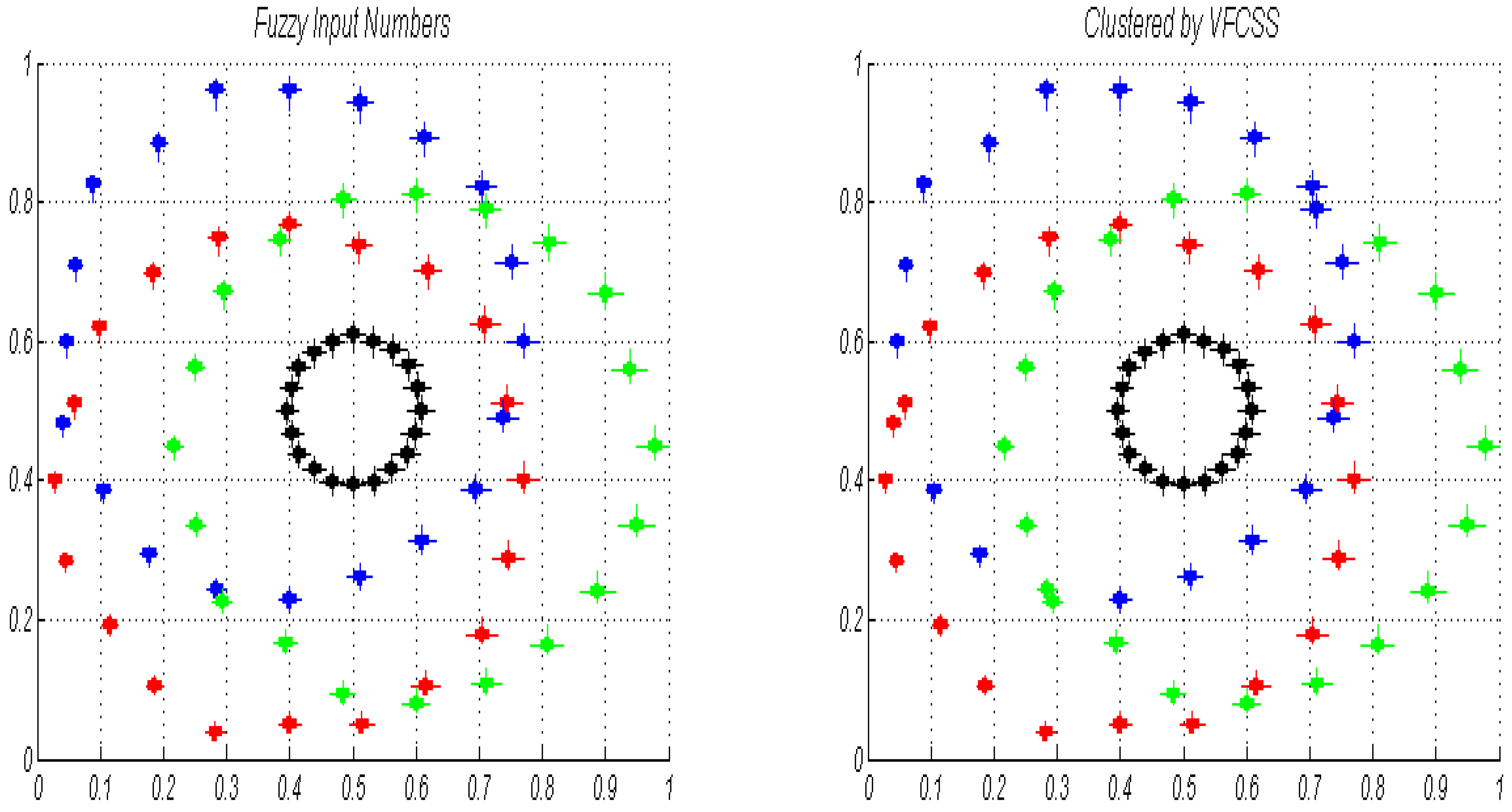
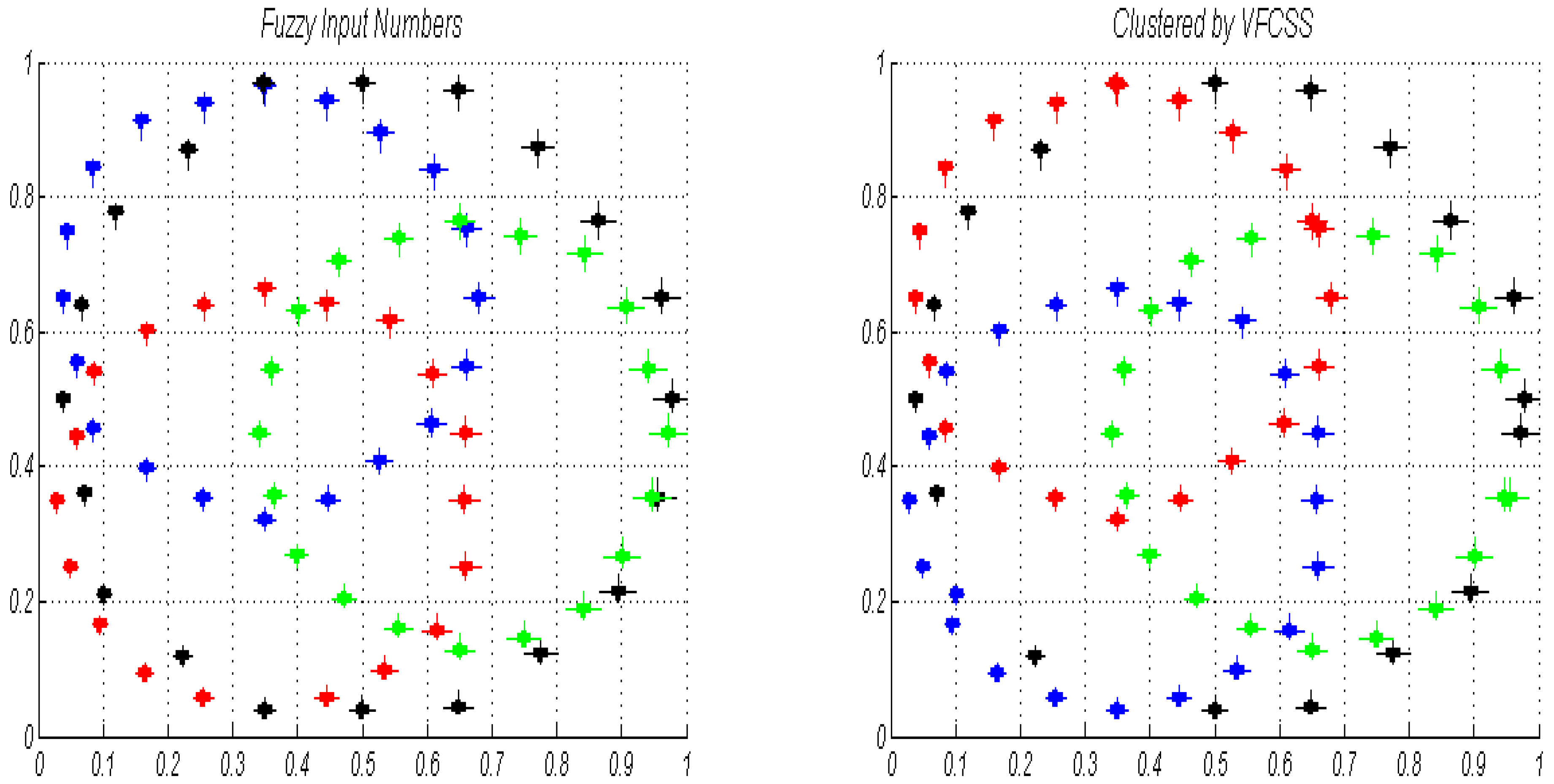
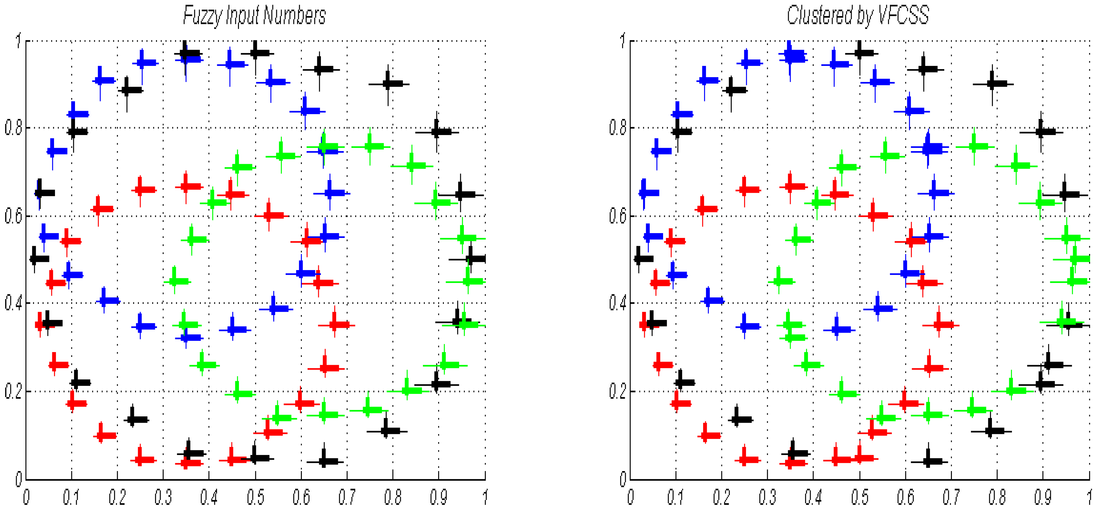
State 1. In the first state, in the first step the proposed VFCSS is applied to four classes of numbers that are overlapping. The simulation result for this step is provided in Figure 2. In the second step, VFCSS is applied to four classes of numbers that are complex and overlapping. The simulation result for this step is provided in Figure 3. The CM of these two steps is expressed in

Table 9. CM of VFCSS applied over LR-type fuzzy numbers of Figure 2 and Figure 3 (first and second steps of state 1).

	Step	First Step	Second Step
Output Clusters
Confusion Matrix		$\left[\begin{array}{c}20,0,0,0\\ 1,18,0,1\\ 0,0,20,0\\ 0,1,0,19\end{array}\right]$	$\left[\begin{array}{c}20,0,0,0\\ 0,20,0,0\\ 2,1,16,1\\ 0,1,1,18\end{array}\right]$

.

State 2. In this state, the input fuzzy numbers are not symmetric. On the other hand, we do not use from (41) to create fuzzy numbers. The procedure for producing fuzzy numbers in this state is as follows:

$${\widetilde{ x}}_{k,j}={\left(x_{k,j}-0.01,x_{k,j}+0.03,0.04x_{k,j},0.02x_{k,j}\right)}_{LR}$$

(42)

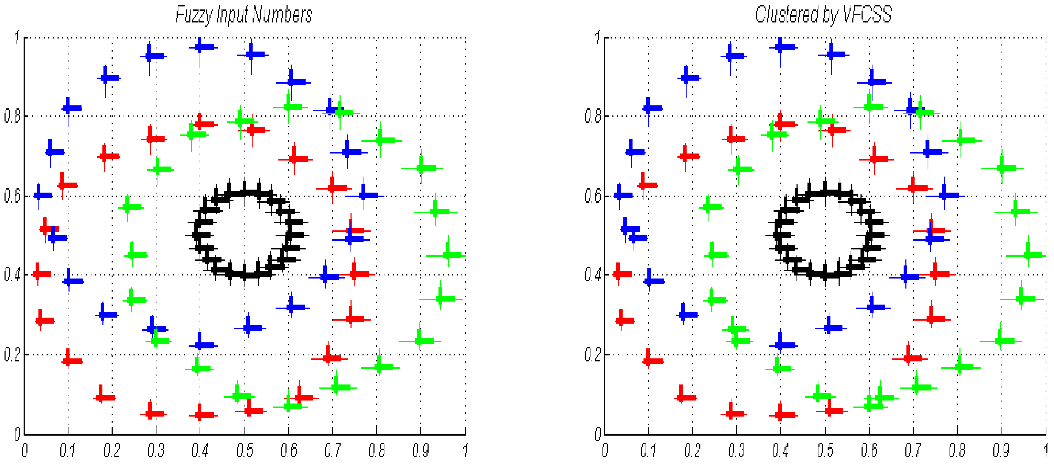
In this state, we apply VFCSS clustering over LR-type fuzzy numbers with the same conditions as for state 1. Simulation results of the corresponding two steps of this state are demonstrated in Figure 4 and Figure 5. The CM of these two steps is expressed in

Table 10. CM of VFCSS applied over LR-type fuzzy numbers of Figure 4 and Figure 5 (first and second steps of state 2).

	Step	First Step	Second Step
Output Clusters
Confusion Matrix		$\left[\begin{array}{c}18,1,0,1\\ 0,19,0,1\\ 0,0,20,0\\ 0,0,0,20\end{array}\right]$	$\left[\begin{array}{c}20,0,0,0\\ 0,19,0,1\\ 1,2,15,2\\ 0,1,2,17\end{array}\right]$

.

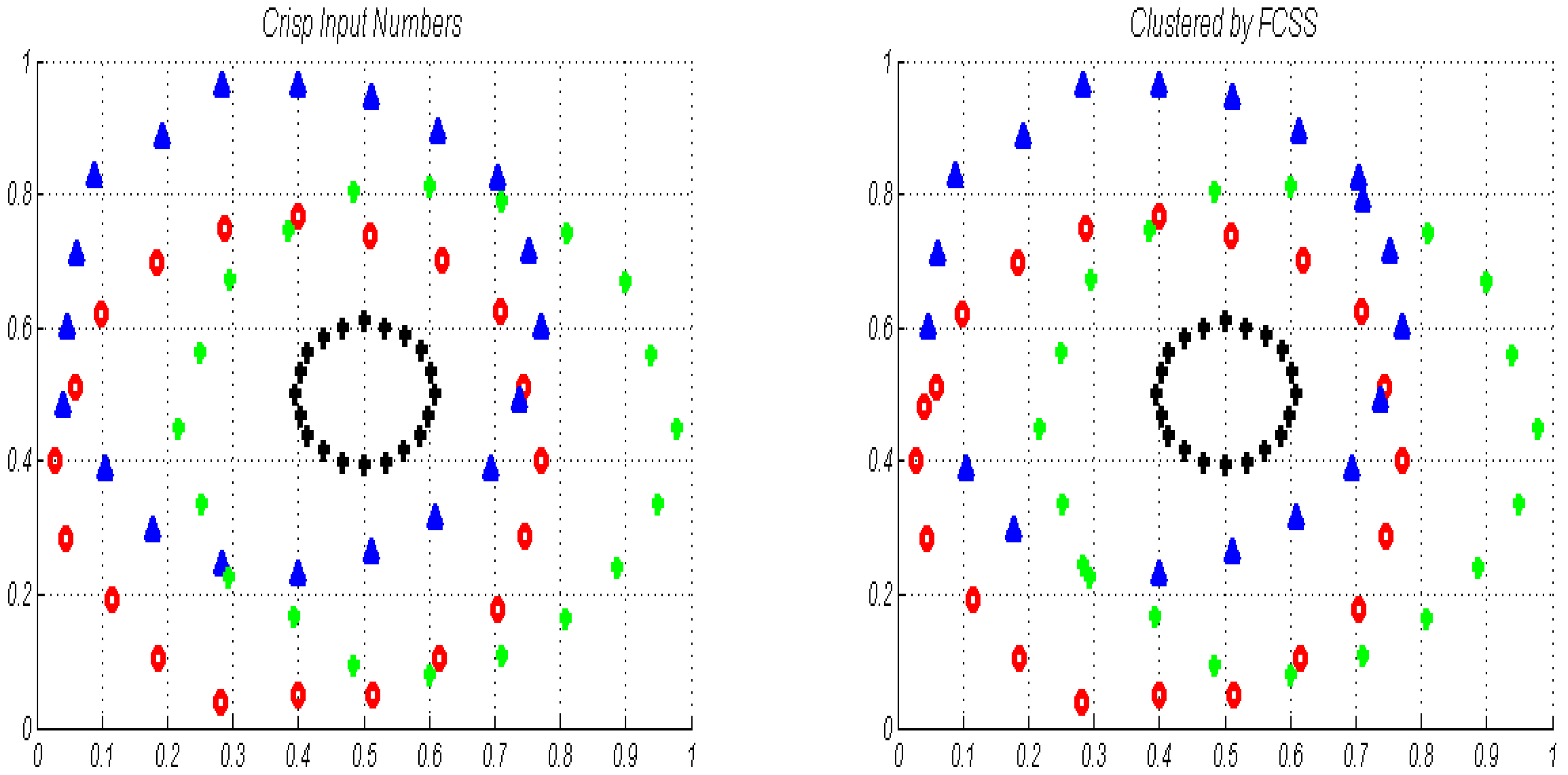
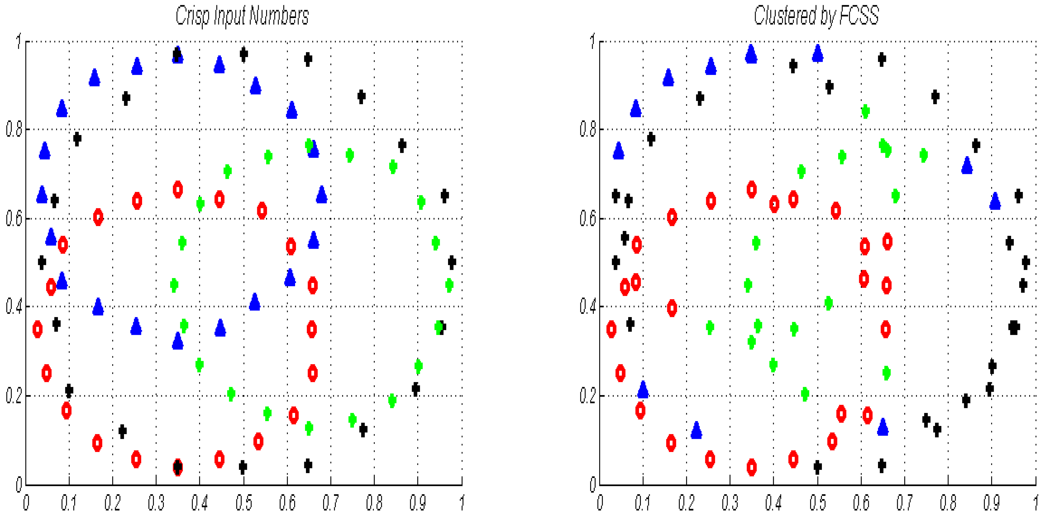
State 3. In the third state, as we can represent an LR-type fuzzy number with its mean ($\left(m_1+m_2\right)/2$ from 41) as a crisp number, we apply a similar condition as for the two previous states for crisp numbers. Therefore, conventional FCSS is applied over input crisp numbers. Simulation results for the corresponding two steps of this state are demonstrated in Figure 6 and Figure 7. The CM of these two steps is expressed in

Table 11. CM of VFCSS applied over crisp numbers of Figure 6 and Figure 7 (first and second steps of state 3).

	Step	First Step	Second Step
Output Clusters
Confusion Matrix		$\left[\begin{array}{c}20,0,0,0\\ 1,18,0,1\\ 0,0,20,0\\ 0,1,0,19\end{array}\right]$	$\left[\begin{array}{c}8,7,4,1\\ 7,8,3,2\\ 1,0,19,0\\ 0,1,1,18\end{array}\right]$

.

In this state it is observed, in the first step, the performance of the proposed VFCSS (first step of state 3) and FCSS (first step of state 5) clustering methods are similar. While in the second step, the proposed VFCSS can cluster input numbers well, while the conventional FCSS cannot do this as well. Although in the simulation results the procedure of producing fuzzy numbers is very simple and primary. Performance of the proposed VFCSS can be improved further by a change in the procedure of producing fuzzy numbers (41), as well.

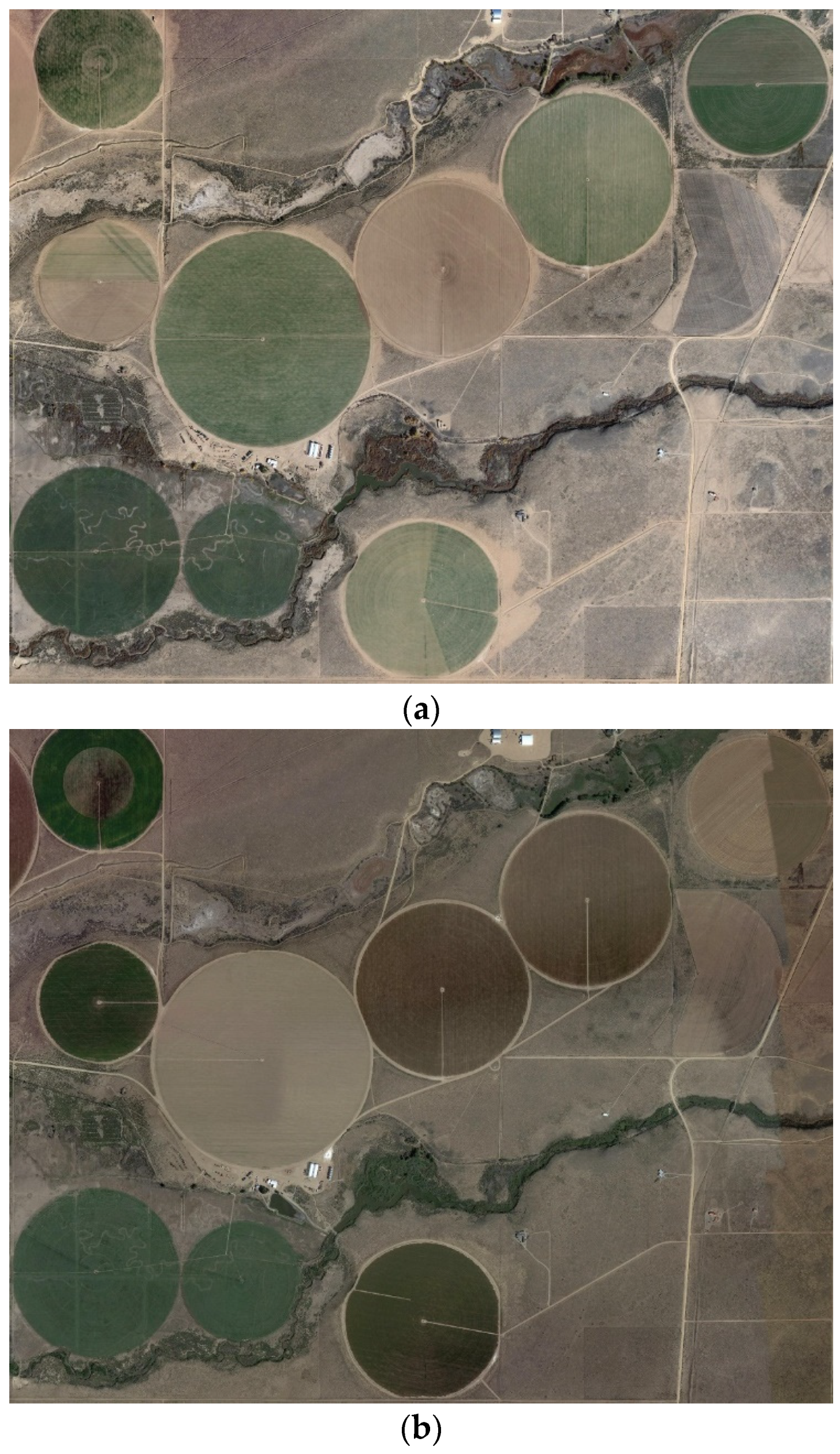
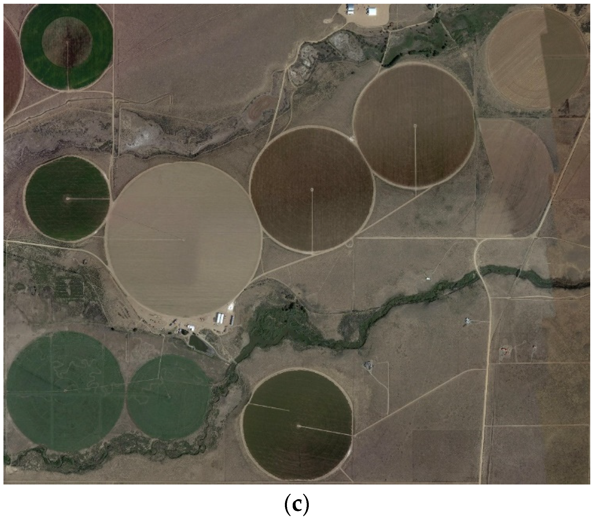
State 4. In the last state, the application of the proposed model is illustrated in real life. Geomorphology science and remotely sensed images are selected for simulation in this state. Geomorphology is the study of landforms dealing with the terrain relief. It is the morphology of the earth surface that works as the basic element separating geomorphology into an autonomous science in the Earth sciences. By analyzing the geometry of landforms, it is possible to study the relief and its properties from a validated perspective using mathematical apparatus [34]. Furthermore, remotely sensed imagery has been used widely in geomorphology due to the availability of satellite data, with its value measurable by the point to which it can meet the investigative needs of geomorphologists. Geomorphologists are therefore concerned with the Earth surface geometry and composition of the terrain relief. They use this information to determine presently operating processes, as well as predictive prior landforms and the events. They try to model geomorphological processes and use a wide range of techniques to predict future land surface change [35]. Therefore, in this paper, three georeferenced satellite images (obtained using Google maps) illustrated in Figure 8 are utilized, where they are related to the US with coordinates (Upper Left: 37°24′10″N, 105°35′12″W and Lower Right: 37°22′30″N, 105°32′35″W). These images are used to estimate the area of the agricultural fields (by estimating the circle radius values). For this purpose, using Arc GIS 10.5 software, the circles are extracted with the clip tool.

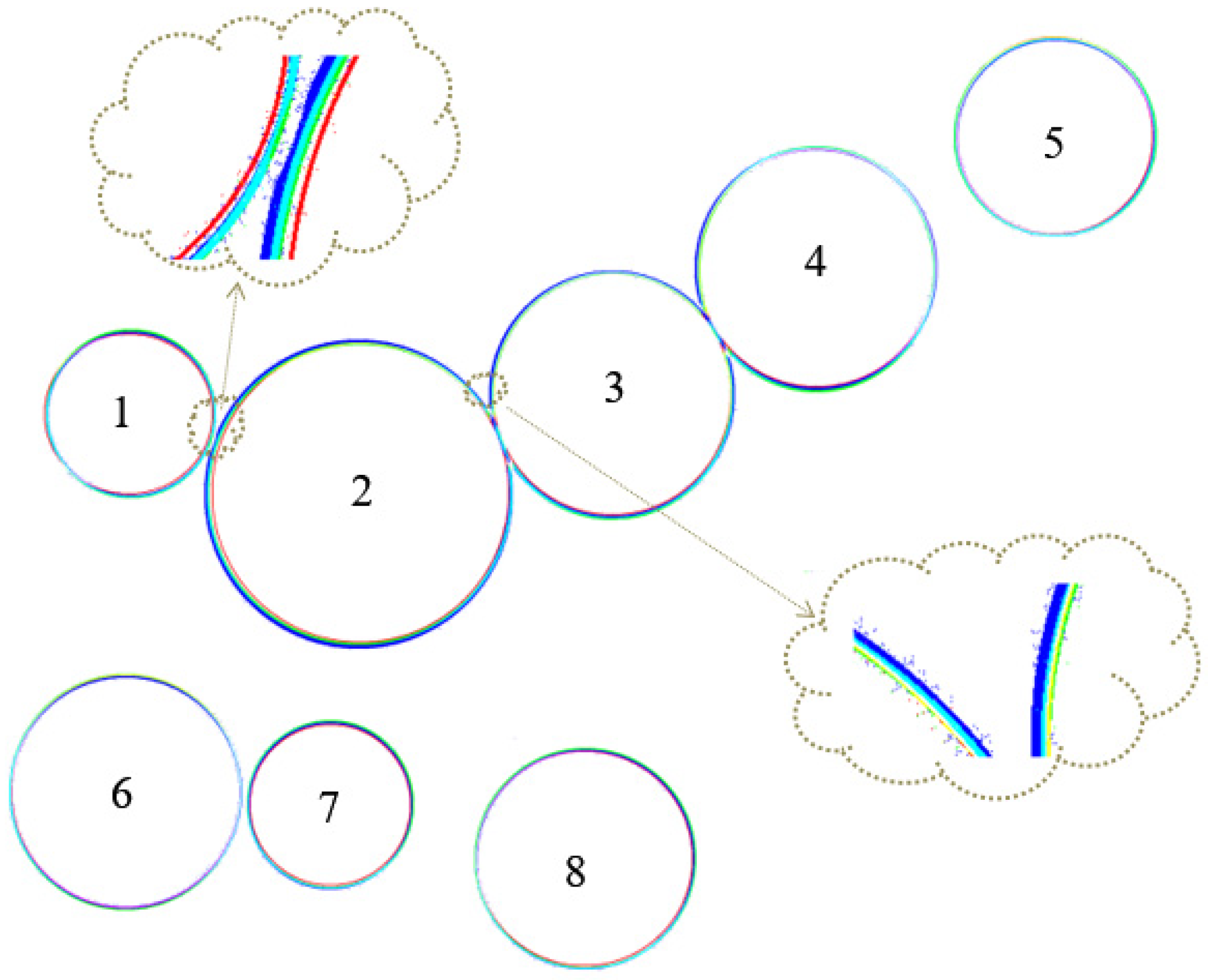
If we demonstrate the extracted circles from images (a), (b) and (c) of Figure 8 by red, green and blue color respectively, the resulting circles are as in Figure 9. It can be observed, some of the resulting circles are non-overlapping while in some areas, as in the worst case, all 3 circles are in contact and are specified by red, green, and blue colors. In some area, two colors from RGB overlap and combined and cyan, yellow, and pink colors result. Finally, in rare cases, by complete overlapping of the circles, white color results. For this case, the resulting radius by conventional FCSS is reported in

Table 12. Simulation results for state 4 and comparison of resulting radii with FCSS and VFCSS algorithms.

Circle No Radius	1	2	3	4	5	6	7	8
Result by applying FCSS on image (a) Figure 8	205	377	301	310	250	285	201	268
Result by applying FCSS on image (b) Figure 8	212	380	307	314	258	297	211	279
Result by applying FCSS on image (c) Figure 8	210	385	315	318	257	291	209	274
Result by VFCSS	209	381	306	315	255	293	208	274

. We can observe various values for each circle are obtained by conventional FCSS (in an un-regular manner, it means the resulting radius from the first image in some cases is the min value, in other cases is the max value, etc.). This ambiguity will be increased, by increasing the number of available images. Furthermore, computational complexity will be increased by growing the number of available images as well. For this reason, FCSS must be applied on image circles separately.

However, on the other side, the proposed VFCSS method is applied on the resulting fuzzy numbers and circles for three images of Figure 9 (considering the fuzzification process of [36] and associated interval-symbolic numbers for each circle’s pixels). Simulation results (reported in Table 12) show only one acceptable and moderate value for each circle; even by increasing the available images that leads to more exact and nearer to the true radius value (see [36]). Furthermore, the computation complexity in the proposed method is very low, fixed, and equivalent with one time applying the FCSS, even by increasing the available number of images.

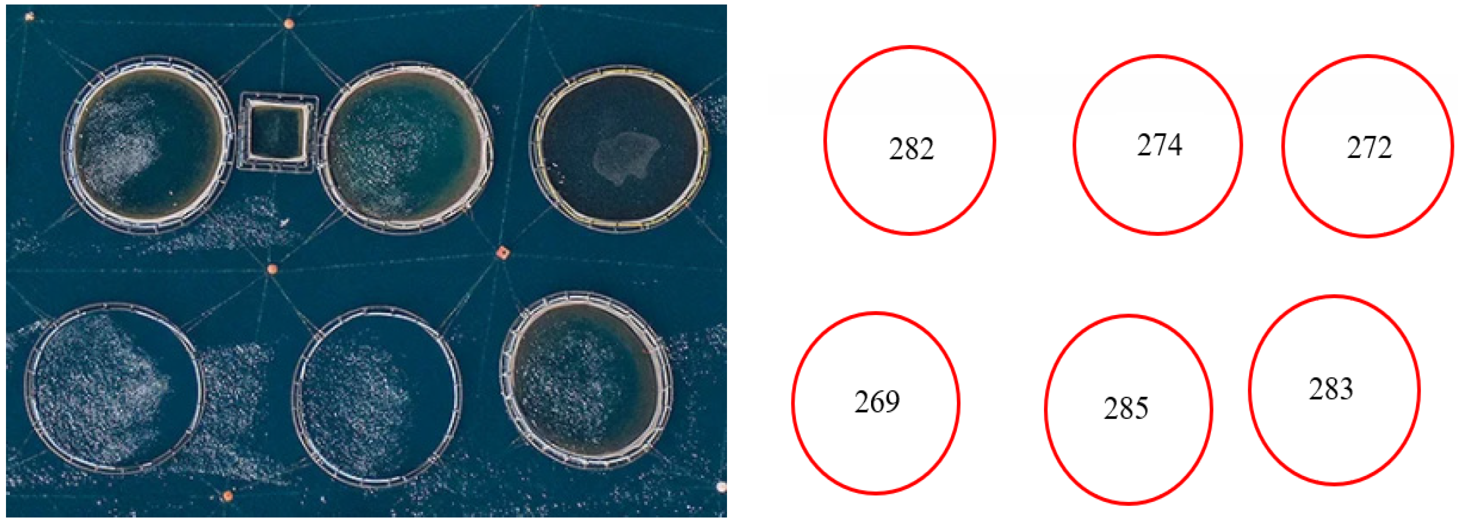
For more remote sensing applications, Figure 10 shows the proposed model results on a fish farm satellite image which is captured as Aquaculture farms off the coast of Greece by Bernhard Lang [37]. The extracted circles and simulation results for circles radii with VFCSS algorithm are shown. It should be noted that the fuzzy-related works can be utilized without accessing a big dataset and just by a single image. These models can be applied directly without any training and validation processes. The proposed model is a new fuzzy clustering model which can be utilized for remote sensing applications. This fuzzy model can be helpful for designing smart image processing systems. For lower-quality images, it just is needed to add some simple preprocessing (noise removal, adjustment, etc.) to have a high-quality image for the proposed model.

4. Conclusions

In this paper, a vector form of fuzzy c-spherical shells clustering (VFCSS) has been proposed. We can cluster non-crisp numbers that have spherical shells form using the proposed VFCSS. These non-crisp numbers can be available, or we can produce them from crisp number. It has been shown that we can improve the performance of conventional fuzzy c-spherical shells clustering over crisp numbers using the proposed VFCSS. This fact can be obtained by choosing a suitable procedure for producing non-crisp (fuzzy) numbers from crisp numbers. Furthermore, simulation results show better performance and low-cost computational complexity of the proposed VFCSS method versus the conventional FCSS in real life application in morphology science. We implement our clustering model over various types of geomorphology images for extracting the radii of circular agricultural fields using remotely sensed images and, we applied our model on these types of images to show that this clustering model can be utilized for remote sensing applications. To apply new deep learning models on an application we need a big and proper dataset to train, valid and test the models. The main uniqueness of fuzzy-related works is that we can utilize them without accessing a big dataset. We can use these models directly without any training and validation processes. Our model is a new fuzzy clustering model which can be utilized for remote sensing wapplications.

References

- Bellman, R.; Kalaba, R.; Zadeh, L.A. Abstraction and Pattern Classification. J. Math. Anal. Appl. 1966, 13, 1–7. [Google Scholar] [CrossRef]
- Bezdek, J.C. Pattern Recognition with Fuzzy Objective Function Algorithms; Kluwer Academic Publishers: New York, NY, USA, 1981. [Google Scholar]
- Yang, M.-S. A survey of fuzzy clustering. Math. Comput. Model. 1993, 18, 1–16. [Google Scholar] [CrossRef]
- MacQueen, J. Some methods for classification and analysis of multivariate observations. In Proceedings of the Fifth Berkeley Symposium on Mathematical Statistics and Probability, Berkeley, CA, USA, 21 June–18 July 1965; Volume 1, pp. 281–297. [Google Scholar]
- Zadeh, L.A. Fuzzy sets. Inf. Control. 1965, 8, 338–353. [Google Scholar] [CrossRef] [Green Version]
- Wu, K.-L.; Yang, M.-S. Alternative c-means clustering algorithms. Pattern Recognit. 2002, 35, 2267–2278. [Google Scholar] [CrossRef]
- Hadi, M.; Morteza, K.; Hadi, S.Y. Vector fuzzy C-means. J. Intell. Fuzzy Syst. 2013, 24, 363–381. [Google Scholar] [CrossRef]
- Hossein-Abad, H.M.; Shabanian, M.; Kazerouni, I.A. Fuzzy c-means clustering method with the fuzzy distance definition applied on symmetric triangular fuzzy numbers. J. Intell. Fuzzy Syst. 2020, 38, 2891–2905. [Google Scholar] [CrossRef]
- Hossein-Abad, H.M.; Shabanian, M.; Kazerouni, I.A. Vectorized Kernel-Based Fuzzy C-Means: A Method to Apply KFCM on Crisp and Non-Crisp Numbers. Int. J. Uncertain. Fuzziness Knowl.-Based Syst. 2020, 28, 635–659. [Google Scholar] [CrossRef]
- Saha, A.; Das, S. On the unification of possibilistic fuzzy clustering: Axiomatic development and convergence analysis. Fuzzy Sets Syst. 2018, 340, 73–90. [Google Scholar] [CrossRef]
- Yu, H.; Fan, J.; Lan, R.; La, R. Suppressed possibilistic c-means clustering algorithm. Appl. Soft Comput. 2019, 80, 845–872. [Google Scholar] [CrossRef]
- Saha, A.; Das, S. Axiomatic generalization of the membership degree weighting function for fuzzy C means clustering: Theoretical development and convergence analysis. Inf. Sci. 2017, 408, 129–145. [Google Scholar] [CrossRef]
- Dave, R. Fuzzy shell-clustering and applications to circle detection in digital images. Int. J. Gen. Syst. 1990, 16, 343–355. [Google Scholar] [CrossRef]
- Dave, R.; Bhaswan, K. Adaptive fuzzy c-shells clustering and detection of ellipses. IEEE Trans. Neural Netw. 1992, 3, 643–662. [Google Scholar] [CrossRef] [PubMed]
- Krishnapuram, R.; Nasraoui, O.; Frigui, H. The fuzzy c spherical shells algorithm: A new approach. IEEE Trans. Neural Netw. 1992, 3, 663–671. [Google Scholar] [CrossRef]
- Man, Y.; Gath, I. Detection and separation of ring-shaped clusters using fuzzy clustering. IEEE Trans. Pattern Anal. Mach. Intell. 1994, 16, 855–861. [Google Scholar] [CrossRef]
- Gath, I.; Hoory, D. Fuzzy clustering of elliptic ring-shaped clusters. Pattern Recognit. Lett. 1995, 16, 727–741. [Google Scholar] [CrossRef]
- Krishnapuram, R.; Frigui, H.; Nasraoui, O. Fuzzy and possibilistic shell clustering algorithms and their application to boundary detection and surface approximation. IEEE Trans. Fuzzy Syst. 1995, 3, 29–43. [Google Scholar] [CrossRef]
- Bezdek, J.C.; Hathaway, R.J.; Pal, N.R. Norm-induced shell-prototypes (NISP) clustering. Neural Parallel Sci. Comput. 1995, 3, 431–449. [Google Scholar]
- Hoeppner, F. Fuzzy shell clustering algorithms in image processing: Fuzzy C-rectangular and 2-rectangular shells. IEEE Trans. Fuzzy Syst. 1997, 5, 599–613. [Google Scholar] [CrossRef]
- Wang, T. Possibilistic Shell Clustering of Template-Based Shapes. IEEE Trans. Fuzzy Syst. 2008, 17, 777–793. [Google Scholar] [CrossRef]
- Song, Q.; Yang, X.; Soh, Y.C.; Wang, Z.M. An information-theoretic fuzzy C-spherical shells clustering algorithm. Fuzzy Sets Syst. 2010, 161, 1755–1773. [Google Scholar] [CrossRef]
- Mahdipour, H.H.-A.; Khademi, M.; Sadoghi, H.Y. Model-based fuzzy c-shells clustering. Neural Comput. Appl. 2011, 21, 29–41. [Google Scholar] [CrossRef]
- D’Urso, P.; Giordani, P. A weighted fuzzy c-means clustering model for fuzzy data. Comput. Stat. Data Anal. 2006, 50, 1496–1523. [Google Scholar] [CrossRef]
- De Carvalho, F. Fuzzy clustering algorithms for symbolic interval data based on adaptive and non-adaptive Euclidean distances. In Proceedings of the 2006 Ninth Brazilian Symposium on Neural Networks (SBRN’06), Ribeirao Preto, Brazi, 23–27 October 2006; pp. 60–65. [Google Scholar]
- de Carvalho, F. Fuzzy c-means clustering methods for symbolic interval data. Pattern Recognit. Lett. 2007, 28, 423–437. [Google Scholar] [CrossRef]
- Chuang, C.-C.; Jeng, J.-T.; Li, C.-W. Fuzzy c-means clustering algorithm with unknown number of clusters for symbolic interval data. In Proceedings of the 2008 SICE Annual Conference, Tokyo, Japan, 20–22 August 2008; pp. 358–363. [Google Scholar]
- Hathaway, R.; Bezdek, J.; Pedrycz, W. A parametric model for fusing heterogeneous fuzzy data. IEEE Trans. Fuzzy Syst. 1996, 4, 270–281. [Google Scholar] [CrossRef]
- Yang, M.-S.; Ko, C.-H. On a class of fuzzy c-numbers clustering procedures for fuzzy data. Fuzzy Sets Syst. 1996, 84, 49–60. [Google Scholar] [CrossRef]
- Yang, M.-S.; Hwang, P.-Y.; Chen, D.-H. Fuzzy clustering algorithms for mixed feature variables. Fuzzy Sets Syst. 2004, 141, 301–317. [Google Scholar] [CrossRef]
- Hung, W.-L.; Yang, M.-S. Fuzzy clustering on LR-type fuzzy numbers with an application in Taiwanese tea evaluation. Fuzzy Sets Syst. 2005, 150, 561–577. [Google Scholar] [CrossRef]
- Yang, M.-S.; Hung, W.-L.; Cheng, F.-C. Mixed-variable fuzzy clustering approach to part family and machine cell formation for GT applications. Int. J. Prod. Econ. 2006, 103, 185–198. [Google Scholar] [CrossRef]
- Rong, L.; Jiu-lun, F. A Fuzzy C-means Type Clustering Algorithm on Triangular Fuzzy Numbers. In Proceedings of the Sixth International Conference on Fuzzy Systems and Knowledge Discovery, Tianjin, China, 14–16 August 2009. [Google Scholar]
- Lopatin, D.V.; Zhirov, A.I. Geomorphology in the system of Earth sciences. Geogr. Nat. Resour. 2017, 38, 313–318. [Google Scholar] [CrossRef]
- Smith, M.; Pain, C. Applications of remote sensing in geomorphology. Prog. Phys. Geogr. Earth Environ. 2009, 33, 568–582. [Google Scholar] [CrossRef]
- Hadi, S.Y.; Morteza, K. Efficient Land-cover segmentation using Meta fusion. J. Inf. Syst. Telecommun. (JIST) 2016, 4, 152–166. [Google Scholar]
- Lang, B. Aquaculture Farms off the Coast of Greece. Available online: https://www.wired.com/story/the-fantastic-geometry-of-greeces-fish-farms-2000-feet-up/ (accessed on 20 May 2017).
Figure 1.
Parameterization of TFN.
Figure 2.
Proposed VFCSS clustering over input LR-type fuzzy numbers include four interference classes red, blue, black and green with (20,20,20,20) members, (first step of state 1).
Figure 3.
Proposed VFCSS clustering over input LR-type fuzzy numbers include four complexity interference classes red, blue, black and green with (20,20,20,20) members, (second step of state 1).
Figure 4.
Proposed VFCSS clustering over input non-symmetric LR-type fuzzy numbers include four interference classes red, blue, black and green with (20,20,20,20) members, (first step of state 2).
Figure 5.
Proposed VFCSS clustering over input non-symmetric LR-type fuzzy numbers include four complexity interference classes red, blue, black and green with (20,20,20,20) members (second step of state 2).
Figure 6.
Conventional FCSS clustering over crisp input numbers include four interference classes red, blue, black, and green with (20,20,20,20) members, (first step of state 3).
Figure 7.
Conventional FCSS clustering over crisp input numbers include four complexity interference classes red, blue, black and green with (20,20,20,20) members (second step of state 3).
Figure 8.
Three georeferenced satellite images (obtained using Google maps) obtained over three different dates (a) 23-10-2011 (b) 09-09-2016 (c) 30-12-2018 (used for state 4).
Figure 9.
The extracted circles from images (a), (b) and (c) Figure 8 represented by red, green and blue colors, respectively.
Figure 10.
A fish farm satellite image (Left) and the extracted circles from the image and radii results (Right) using VFCSS algorithm.