Article

Spatial Downscaling of MODIS Snow Cover Observations Using Sentinel-2 Snow Products

by
Jesús Revuelto
1,*,
Esteban Alonso-González
1,2,
Simon Gascoin
2,
Guillermo Rodríguez-López
1,3 and
Juan Ignacio López-Moreno
1
1
Instituto Pirenaico de Ecología, Consejo Superior de Investigaciones Científicas (IPE-CSIC), 50002 Zaragoza, Spain
2
Centre d’Etudes Spatiales de la Biosphère, CESBIO, Univ. Toulouse, CNES/CNRS/INRAE/IRD/UPS, 31000 Toulouse, France
3
Departamento de Geografía y Ordenación del Territorio, Universidad de Zaragoza, 50002 Zaragoza, Spain
*
Author to whom correspondence should be addressed.
Remote Sens. 2021, 13(22), 4513; https://0-doi-org.brum.beds.ac.uk/10.3390/rs13224513
Submission received: 27 September 2021 / Revised: 29 October 2021 / Accepted: 7 November 2021 / Published: 10 November 2021
(This article belongs to the Special Issue Remote Sensing of Water Cycle Science in the Cryosphere)

Abstract

:
Understanding those processes in which snow dynamics has a significant influence requires long-term and high spatio-temporal resolution observations. While new optical space-borne sensors overcome many previous snow cover monitoring limitations, their short temporal length limits their application in climatological studies. This work describes and evaluates a probabilistic spatial downscaling of MODIS snow cover observations in mountain areas. The approach takes advantage of the already available high spatial resolution Sentinel-2 snow observations to obtain a snow probability occurrence, which is then used to determine the snow-covered areas inside partially snow-covered MODIS pixels. The methodology is supported by one main hypothesis: the snow distribution is strongly controlled by the topographic characteristics and this control has a high interannual persistence. Two approaches are proposed to increase the 500 m resolution MODIS snow cover observations to the 20 m grid resolution of Sentinel-2. The first of these computes the probability inside partially snow-covered MODIS pixels by determining the snow occurrence frequency for the 20 m Sentinel-2 pixels when clear-sky conditions occurred for both platforms. The second approach determines the snow probability occurrence for each Sentinel-2 pixel by computing the number of days in which snow was observed on each grid cell and then dividing it by the total number of clear-sky days per grid cell. The methodology was evaluated in three mountain areas in the Iberian Peninsula from 2015 to 2021. The 20 m resolution snow cover maps derived from the two probabilistic methods provide better results than those obtained with MODIS images downscaled to 20 m with a nearest-neighbor method in the three test sites, but the first provides superior performance. The evaluation showed that mean kappa values were at least 10% better for the two probabilistic methods, improving the scores in one of these sites by 25%. In addition, as the Sentinel-2 dataset becomes longer in time, the probabilistic approaches will become more robust, especially in areas where frequent cloud cover resulted in lower accuracy estimates.

1. Introduction

The spatio-temporal evolution of snow cover in mountain areas is relevant for understanding runoff production and improving water management in mountain areas [1,2,3]. It is also important for studying plant and animal phenology [4,5,6], soil erosion [7] and glacier mass balance [8,9]. Moreover, from the global energy budget perspective the snow cover has a determinant role since it can cover large areas and has a very high albedo [10,11]. The importance of snow dynamics has motivated the use of a wide variety of observation systems to retrieve the snowpack evolution, including automatic weather stations, manual acquisitions and remote sensing observations.
Since the early stages of space-borne sensors, many studies have monitored snow distribution in mountain areas on different spatio-temporal scales [12,13,14]. Computing the snow-free/snow-covered pixels from satellite images is the most widespread approach for determining snow cover extent [15,16,17]. This monitoring is achieved through passive sensors operating in the near-infrared and visible electromagnetic bands [18,19,20]. Distinct satellite missions have sensors operating in these bands such as MODIS, AVHRR, Sentinel or Landsat. Nonetheless, there are important differences between these missions in terms of the product that they provide regarding the spatial and temporal resolution, but also the extent of the time series available [17,21]. Landsat Thematic Mapper imagery provides a long-lasting database (the first sensor carried on Landsat 4 was launched in 1982) with 30 m spatial resolution. Landsat has a revisit frequency of 16 days, which can be a major drawback for monitoring the snow cover in mountainous regions mainly due to cloud limitations and the rapid changes of snow extent [17,19]. MODIS imagery has been a breakthrough in monitoring snow cover extent since 2001. Despite its inferior spatial resolution of 500 m [22], the MODIS sensor is onboard two satellites (Terra and Aqua), allowing the acquisition of two images per day in mid-latitude areas [19], and nowadays it provides a long record (two decades) of snow observations [23]. In this way MODIS has enabled the production of climatologies of snow cover evolution all over the world [20,24,25,26]. However, there may be important changes in snow cover properties on scales below 100 m [27,28,29,30], and the MODIS resolution is not enough to relate snow presence or duration to processes such as plant phenology, identification of ecological refuges or the hydrological behavior of snow in small catchments [4,31,32,33,34].
The spatial resolution constraints on MODIS acquisitions were mostly overcome when the Sentinel-2 mission was launched, thanks to the high spatial resolution from 13 bands of the electromagnetic spectrum obtained with two satellites (Sentinel 2A and 2B; [35]). This double satellite configuration renders a 5-day revisit frequency [36], allowing snow cover extent to be retrieved from visible and near-infrared bands at 20 m spatial resolution [35,37]. These Sentinel-2 characteristics have pushed ahead high spatial resolution monitoring of snow cover in mountain areas in the last few years [18,30,38]. However, this later satellite imagery has only been available since late 2015, limiting the development of long-term studies. In addition the 5-day revisit time is still a limitation in areas strongly affected by cloud presence [19,39]. This shows that snow cover monitoring still lacks high spatial resolution observations with a suitable temporal resolution to overcome cloud cover limitations [23,40,41]. With new satellite sensors having some of these weaknesses, investigations aimed at upgrading the already available snow cover satellite imagery are required. In this regard, methods allowing a simple spatial downscaling of the already available MODIS observations may benefit a wide variety of applications.
Different spatial downscaling methods of space-borne observations have been used in distinct environmental studies, including satellite-based methods (fusion methods), methods using geoinformation data and model-based methods (i.e., statistical or land surface models) [42,43]. Separate attempts have also been made to downscale MODIS snow cover products. Through an image fusion algorithm of MODIS bands, [44] were able to provide 250 m grid cell size imagery of snow cover products (reflectance, snow cover fraction, etc.). Additionally, a dynamic time-warping technique has allowed the downscaling of MODIS snow cover products [45]. Through a re-ordering of historical Landsat products, Berman et al. (2018) were able to use daily MODIS observations and match the snow dynamics of individual years, finally providing a 30 m resolution fractional snow cover product. Other works have detailed methodologies to merge snow-covered area products from Landsat Enhanced Thematic Mapper Plus (ETM+) and MODIS sensors to reconstruct the Snow Water Equivalent (SWE) at 1 km spatial resolution [46] or have described a terrain-based downscaling technique to derive very high spatial resolution (30 to 3 m spatial resolution) binary snow presence maps [47].
In this study, a simple methodology is proposed to spatially downscale MODIS snow cover mapping. Through training with Sentinel-2 observations, two approaches for computing probabilities are proposed and evaluated. The methods rely on the high interannual repeatability of snow distribution patterns [48,49], thanks to the strong topographic control of snow distribution at scales below 100–200 m, which remains similar throughout different snow seasons [50,51,52,53]. The two methods exploit the already available database of 20 m spatial resolution Sentinel-2 snow cover maps from the Theia snow collection [18]. Both methods compute the probability of snow occurrence for each Sentinel-2 pixel over particular time periods (seasonal computation), but one of them calculates probabilities in Sentinel-2 pixels independently of each other and the other computes the snow occurrence inside every single MODIS pixel (500 m grid cell size). These probabilities are then used to determine the snow distribution inside partially snow-covered MODIS pixels. The final outputs of these products are 20 m spatial resolution snow distribution maps with a daily frequency, only limited by cloud presence. The two methods were trained and evaluated in three study sites in the Iberian Peninsula with dissimilar characteristics. This evaluation was performed through a leave-one-out validation procedure.

2. Materials and Methods
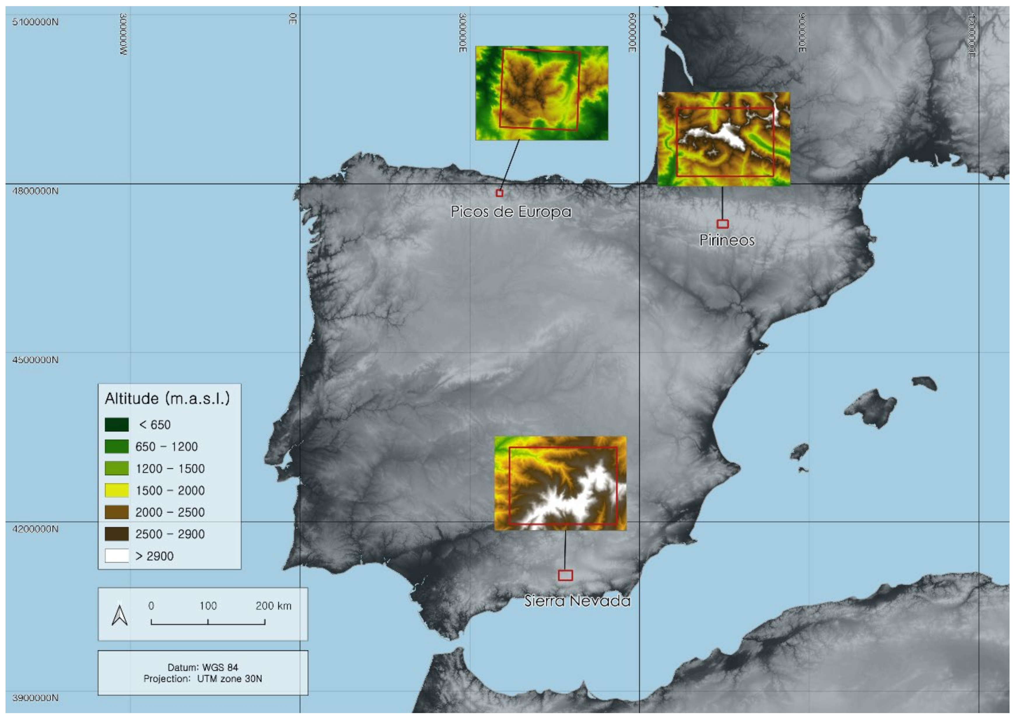
2.1. Study Sites

The three study sites are located in the Iberian Peninsula: the Pyrenees, Sierra Nevada and Picos de Europa (Figure 1). All three exhibit long-lasting snow cover over very complex topography. Nonetheless, their climate and snow dynamics are highly contrasted. The study site located in the Pyrenees encompasses the National Park of Ordesa y Monte Perdido, with elevations between 1060 m a.s.l. (above sea level) and 3350 m a.s.l. This site is characterized by steep U-shaped valleys due to past glacier activity [54,55]. The study area lies in the central Pyrenees between France and Spain (Figure 1). The Pyrenees are characterized by a high interannual variability of snow accumulation [56], and, although high-elevation areas have a remarkable presence of snow throughout the year, lower zones may undergo repeated accumulation and melting events during the snow season [57].
The Sierra Nevada mountain range is located in south-eastern Spain (Figure 1). This range hosts the highest summit of the Iberian Peninsula (Mulhacen Peak), which is less than 40 km from the Mediterranean Sea. In spite of the long-lasting presence of snowpack above 2500–3000 m a.s.l., patchy snow distribution in particular periods is frequent even at high elevation [58]. The elevation gradient of this site ranges from 1230 m a.s.l. to 3479 m a.s.l. This study site comprises nearly the entire National Park of Sierra Nevada.
The National Park of Picos de Europa is a mountain massif in the Cantabrian mountain range. It has a moderate elevation, ranging from 530 m a.s.l. to 2650 m a.s.l. Nonetheless the humid climatic conditions of Picos de Europa produce a long-lasting snow cover in the higher areas [59]. Landscape here is very abrupt, being characterized by steep slopes and numerous large cliffs at the highest elevation.

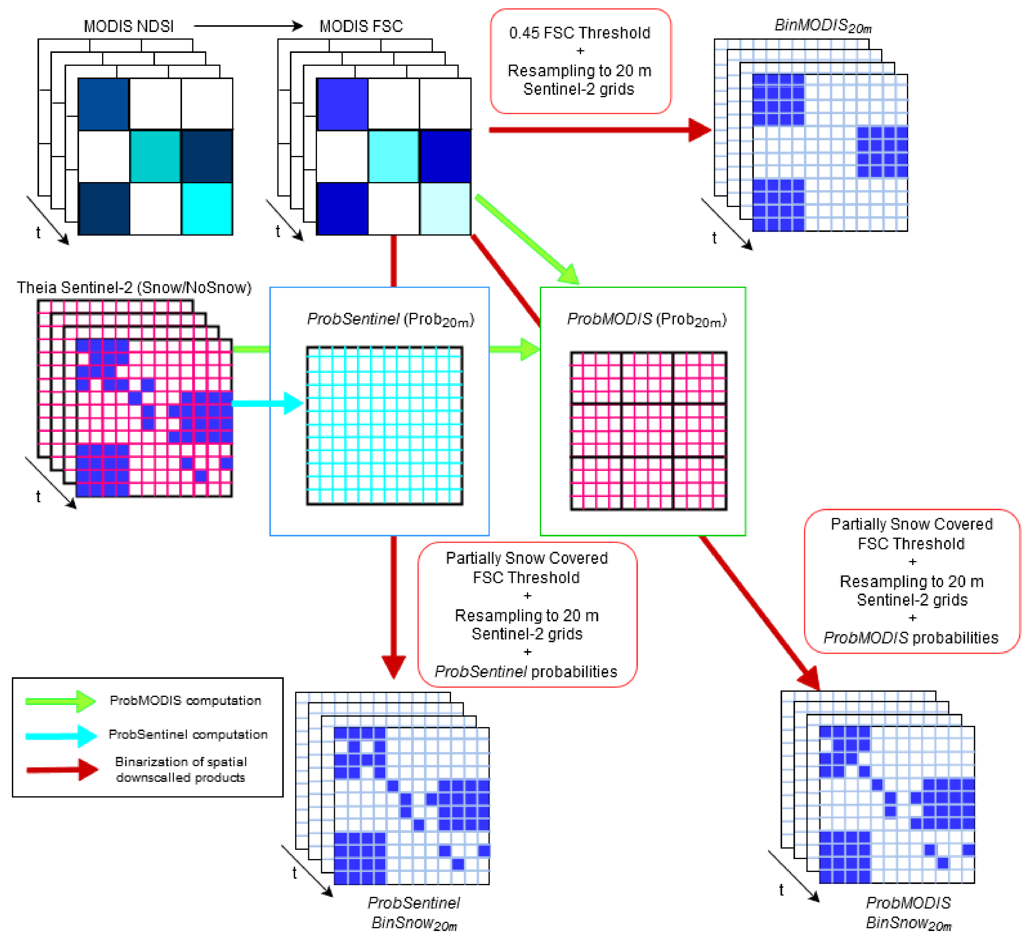
2.2. Probabilistic Spatial Resolution Increase

The methods described here exploit two satellite imageries: the Normalized Difference Snow Index (NDSI) of MODIS 6 and C6.1 products [23,60] and the binary snow occurrence maps of the Theia snow collection from Sentinel-2 [18]. Cloudy areas are masked in the NDSI imagery downloaded from the EathData NASA database [60]. Unlike the NDSI of MODIS, which is a measure of the relative magnitude of the characteristic reflectance difference between the visible and shortwave infrared reflectance [22], Theia is a binary database rendering 1 for snow-covered pixels, 0 for snow-free pixels and NoData in case of cloud (or cloud shadow occurrence). From the available Theia imagery, the snow occurrence probabilities were derived as described below. To provide an easier interpretation of the snow-covered area fraction of MODIS pixels, the Fractional Snow Cover (FSC) was derived from the NDSI through a universal equation (Equation (2) in [61]).
Two approaches are proposed to determine the snow occurrence probability (Prob20m). Later Prob20m is used to classify partially snow-covered MODIS pixels downscaled to 20 m as snow covered or snow free. One approach computes the snow probability inside each MODIS pixel (hereafter ProbMODIS) and the other is computed for the entire Sentinel-2 tile (hereafter ProbSentinel).
ProbMODIS: This procedure yields a snow probability occurrence (Prob20m), based on the snow distribution observed when MODIS pixels were partially snow-covered during a specific training period. The method computes Prob20m inside each native MODIS pixel (500 m), independently of the rest of the MODIS pixels. For MODIS and Sentinel-2 contemporary dates, the snow occurrence probability was computed for all cloud-free MODIS pixels having completely cloud-free Sentinel-2 pixels inside, and in which the MODIS FSC was between the upper and lower thresholds. Prob20m was simply the result of summing up the number of times that each Sentinel-2 pixel was snow-covered and dividing by the total number of times that the entire MODIS pixel was partially snow-covered. This probability may also be interpreted as the probability of a Sentinel-2 pixel being snow-covered divided by the probability of a MODIS pixel being partially snow-covered (see Appendix A for further assessment on probabilities).
ProbSentinel: In this case, only the Theia snow collection images for a particular time period were used to determine Prob20m. This method computes the probability of a particular pixel being snow-covered by simply summing up all days with snow occurrence and dividing this value by the total number of cloud-free observations for this pixel. ProbSentinel probability matches the definition of the Snow Persistence index proposed by [30] for Landsat-8 and Sentinel-2 observations.
The code with a complete example to compute ProbMODIS and to determine the snow occurrence distribution from daily MODIS FSC is provided in the repository https://github.com/ealonsogzl/ProbModis (accessed on 10 October 2021). All cloud-covered MODIS and Sentinel-2 pixels are considered as NoData and thus are not considered for computing probabilities, nor for deriving the spatial downscaled MODIS snow observations. Nonetheless ProbMODIS routines allow the filling of missing Terra values due to cloud presence with Aqua observations of these are available for the same acquisition day, the option used here after in this research.
The final output of the methodology consists of 20 m resolution binary (BinSnow20m) snow cover maps (Snow (1)/NoSnow(0) or NoData). First, 500 m MODIS pixels are resampled to the 20 m Sentinel-2 grid with these requirements; if the FSC of an original MODIS pixel exceeds or does not reach a given upper or lower threshold, all BinSnow20m pixels inside will be respectively considered as snow-covered or snow-free. For FSC between the upper and lower thresholds (determined with a sensitivity test for each test site), the probability of snow occurrence for each 20 m pixel (Prob20m) is used to assign pixels as snow-free or snow-covered. Hereby, Prob20m probabilities inside each 500 m pixel are sorted, and the higher probabilities are then assigned as snow-covered until the number of snow pixels renders the FSC. If two or more Prob20m have the same probability value, a second sorting criterion is applied. This criterion sorts pixels with the same probability by elevation, from higher to lower, and those with higher elevations are assigned as snow-covered. Hence, in partially snow-covered MODIS pixels, the sum of all 20 m snow-covered pixels (BinSnow20m=1) divided by the total number of Sentinel-2 pixels inside the original 500 m MODIS raster is identical to the original FSC value. Figure 2 shows the flow chart for generating the spatially downscaled MODIS snow observations.

2.3. Evaluation Metrics

The performance of both methods was evaluated with three error metrics: the Kappa coefficient, the percentage of agreement (Agree), and the total snow-covered area error. All evaluations described below have excluded forested areas, which were masked, and were computed for days having concurrent MODIS and Sentinel-2 acquisitions.
The Kappa coefficient [62] is a broadly used coefficient in the remote sensing community [24,63,64,65,66] and is widely used in a natural resources context [67]. This coefficient evaluates the agreement beyond chance between a reference and the target to be evaluated. The Kappa coefficient is estimated from a confusion error matrix [68]. In a binary classification, such as that evaluated here, the confusion matrix summarizes all possible scenarios with four elements: true positive, false positive, true negative, and false negative, which respectively correspond to a pixel classified as snow when there is snow, classified as snow when there is no snow, classified as no snow when there is no snow, and classified as no snow when there is snow. From the proportion of cases correctly classified (Po, which may be interpreted as the overall accuracy) and those correctly classified by change (Pe; [62]), the Kappa coefficient is derived using the expression;
κ = P 0 P e 1 P e
The percentage of agreement (Agree) is computed by dividing the number of times that two variables agree by the total number of samples considered. The computation of Agree is rather simple and although it does not evaluate the agreement by chance, this estimate is a good indication of the similarity between the product and the reference.
Kappa and Agree were obtained with the irr package R (https://cran.r-project.org/web/packages/irr/irr.pdf accessed on 10 October 2021), omitting missing data and thus avoiding the evaluation of cloud-covered pixels in any products compared. These two indexes allow a good evaluation of the temporal and spatial evolution of the snow-cover mapping performance of ProbMODIS and ProbSentinel.
In order to evaluate the improvement of the spatial resolution increase based on the snow occurrence probability and a MODIS binarization (Snow/NoSnow), these error estimates were also obtained for increased spatial resolution MODIS images (hereafter BinMODIS20m). This directly rescales to 20 m the 500 m MODIS values using a nearest-neighbor algorithm and then classifies the 20 m pixels as snow-free or snow-covered based on an FSC threshold (note this threshold is different to those used in the probabilistic binarization). Instead of using a threshold from the existing literature, a sensitivity test was conducted to determine which is the FSC value that renders a better snow cover mapping when compared to the Sentinel-2 snow cover map.
As the only 20 m spatial resolution observation of snow distribution is the Sentinel-2 imagery, and this database is also exploited to generate the probabilities with the two methods proposed here, a leave-one-out cross-validation [69] was applied. This method involves the division of the original dataset into N subsets. The model is trained N times with the N − 1 subsets and tested in the remaining N subset. In this case study, the Sentinel-2 imagery is divided into snow seasons (from early September to late July) and thus the evaluation of the ProbMODIS and ProbSentinel is performed with Sentinel-2 images not included in the probability training.
In addition to the Kappa coefficient and Agree, the absolute snow-covered area error was computed to determine if the probabilistic spatial resolution increase of MODIS snow products (either ProbMODIS or ProbSentinel) shows a marked improvement when mapping at the regional scale. The absolute difference between the Sentinel-2 snow-covered area and that obtained with the two methods and BinMODIS20m (the directly increased resolution MODIS binary classification) was determined.

3. Results

The spatial distribution of the snow occurrence probabilities (Prob20m) accounts for the weight that topography has on the snow distribution in mountain areas. This can be observed for the spatial distribution of ProbMODIS probabilities computed for the entire database of Sentinel-2 imagery in the three study areas (Figure 3). In this way, valleys, ridges and mountain summits can be identified in the snow occurrence probability maps.

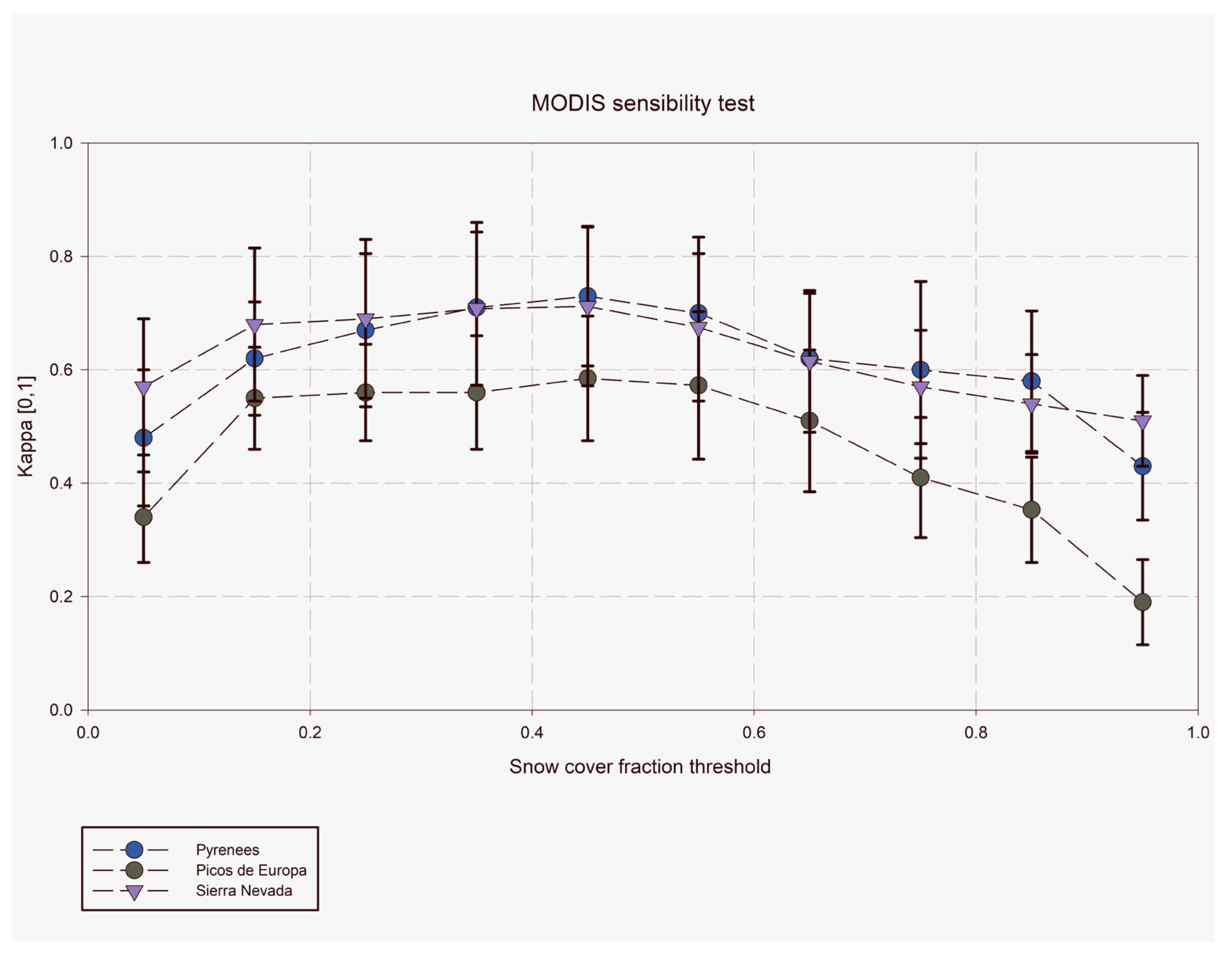
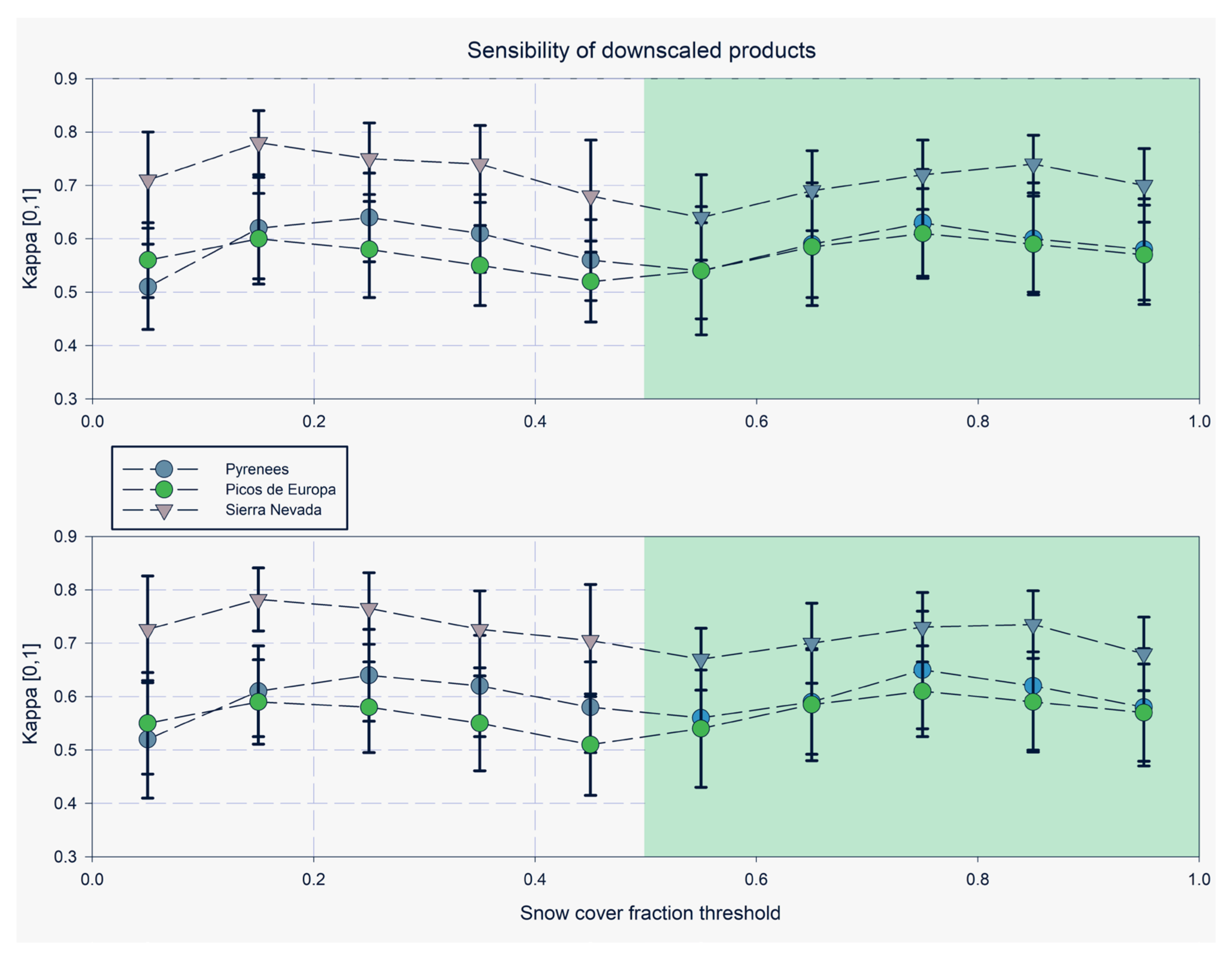
3.1. Sensitivity Test of FSC Thresholds

The sensitivity test to determine the optimal FSC threshold (Figure 4) to classify the BinMODIS20m pixels as snow-free or snow-covered, yielded 0.45 for the three test sites. This sensitivity test comprised all concurrent MODIS and Sentinel-2 images since the later satellite mission became operational. For days with cloud coverage (intersection of MODIS and Sentinel-2 cloud coverage) below 90%, the Kappa value was computed in the cloud-free area. Although a 0.45 FSC threshold is used hereafter to binarize snow presence/absence in the 20 m rescaled MODIS snow cover maps, FSC values ranging from 0.35 to 0.55 render nearly the same results.
The determination of FSC thresholds to consider the 500 m MODIS pixels as snow-free, partially snow-covered or totally snow-covered, in order to then apply ProbMODIS or ProbSentinel probabilities, was assessed through a paired sensitivity test (to compute the upper and lower thresholds). As in the BinMODIS20m sensitivity test, the Kappa values for both methodologies were obtained in the intersection of cloud-free areas for dates having concurrent Sentinel-2 and MODIS acquisitions with cloud coverage less than 90%. Figure 5 depicts the mean Kappa coefficients for the FSC thresholds in the three test sites and for both methodologies. The sensitivity test shows that for the three test areas different upper and lower thresholds are required. For the Pyrenees, both ProbMODIS and ProbSentinel had lower–upper thresholds of 0.25–0.75 respectively, 0.15–0.85 for Sierra Nevada and 0.15–0.75 for Picos de Europa, respectively. Table 1 summarizes the intervals defined with these thresholds.

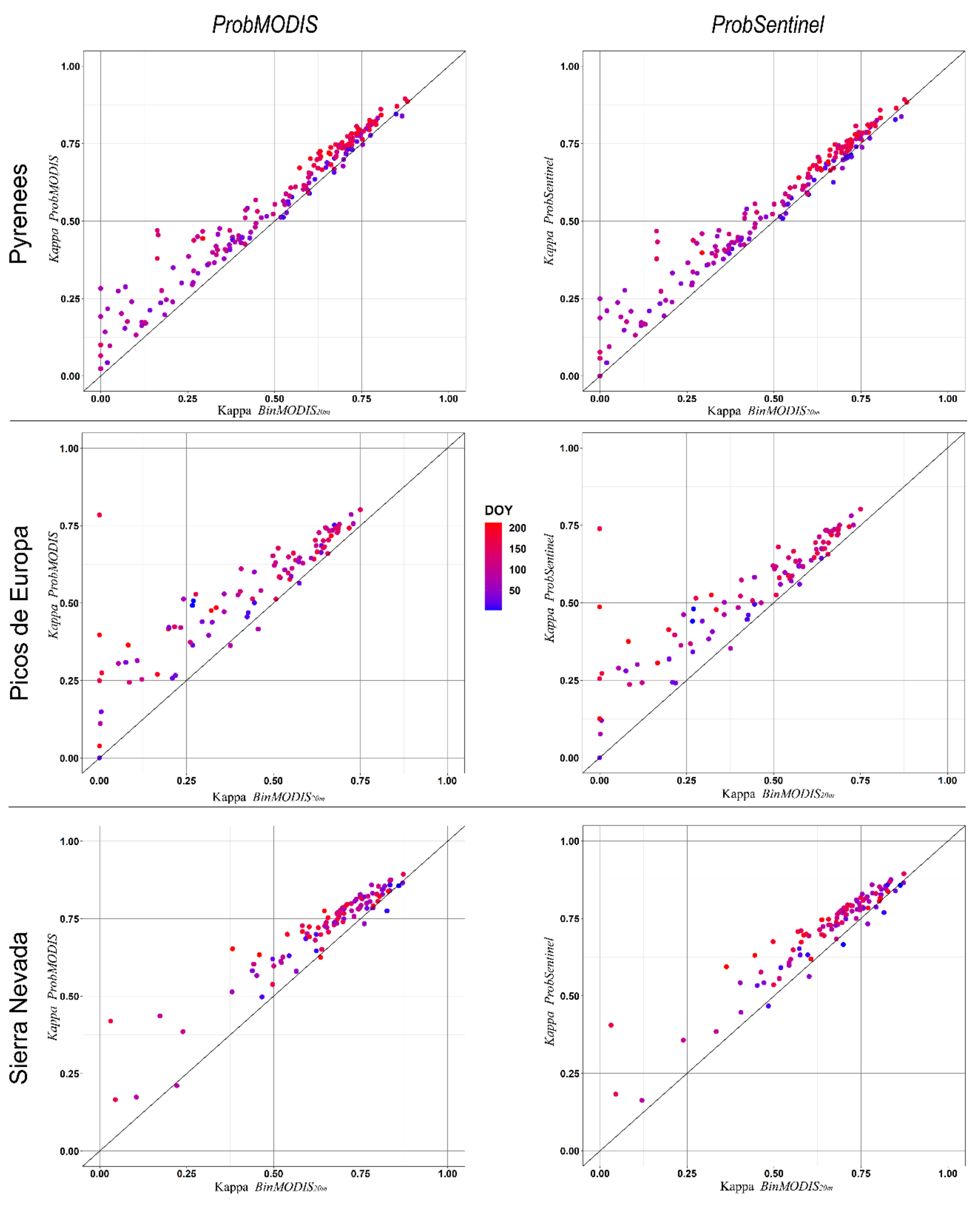
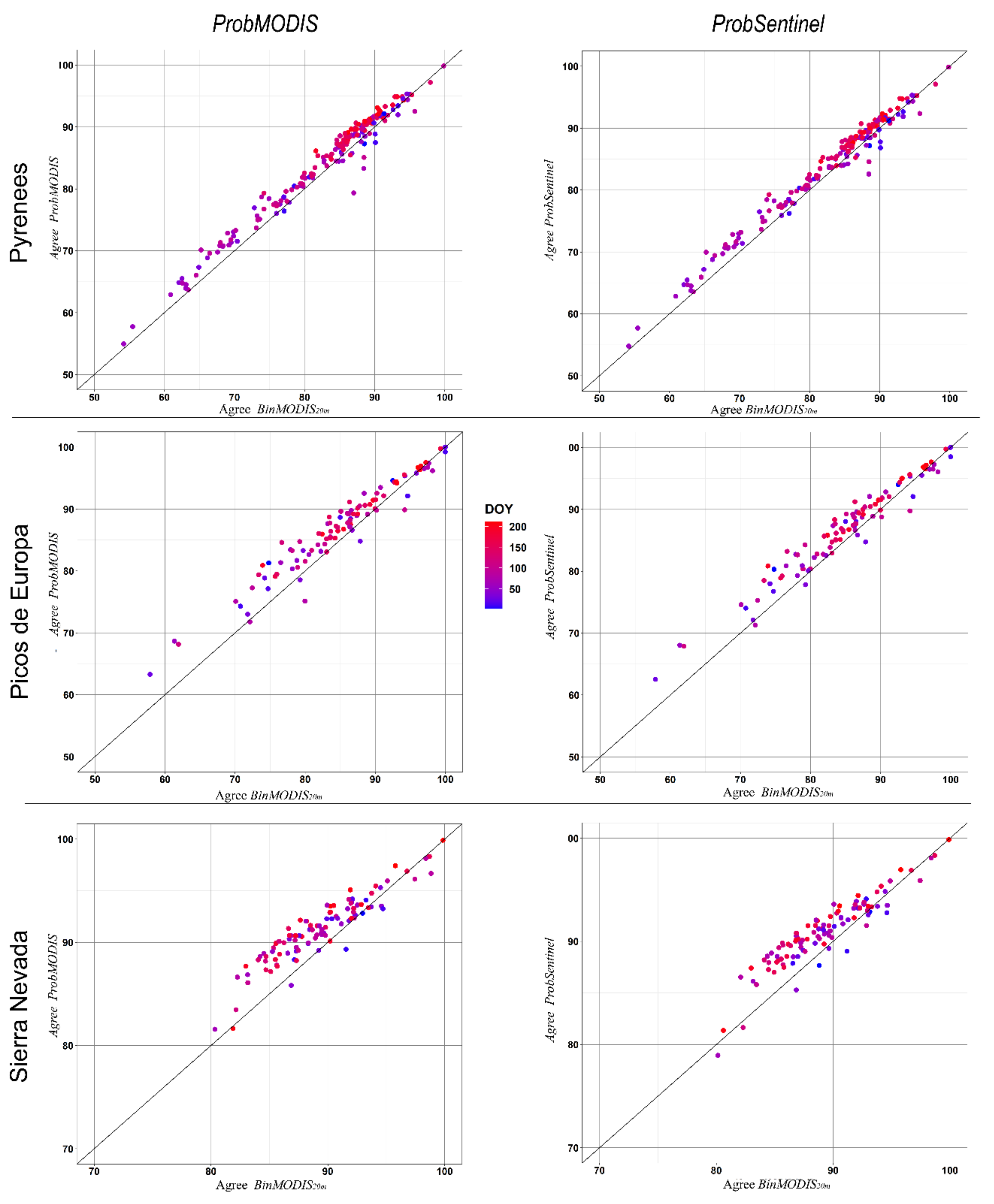
3.2. Daily Improvement of the Probabilistic Snow Occurrence Distribution

Figure 6 and Figure 7 show the scatter plot of the two bias estimates, obtained for each day with ProbMODIS/ProbSentinel probabilities versus that obtained with BinMODIS20m. Nearly all points are above the 1:1 line, showing that the spatial resolution increase based on the snow occurrence probability improves snow-cover mapping. However, for a small fraction of days the methodology fails and produces worse results. These days are generally found at the beginning of the snow season (dark blue) when the snow distribution may not be strongly controlled by the topography. Conversely, late snow season days show a marked improvement in Kappa coefficient values (Figure 6). Similarly, the percentage of agreement (Figure 7) has a similar behavior and shows an improvement as the snow season advances (dark blue to red colors transition). Again, with a distinct error indicator (in this case the percentage of agreement, Figure 7), it is revealed that the spatial distribution of the snow covered pixels obtained with ProbMODIS or ProbSentinel probabilities better captures the true snow cover distribution.
In the three test sites, the two error estimates (Kappa and Agree) for ProbMODIS and ProbSentinel provide better average results than BinMODIS20m observations, and also lower standard deviations, showing the overall improvement of the methodology (Table 2). The average improvement obtained for Kappa is at least 10% for the two probabilistic methods, improving the scores obtained in Picos de Europa by 25%.

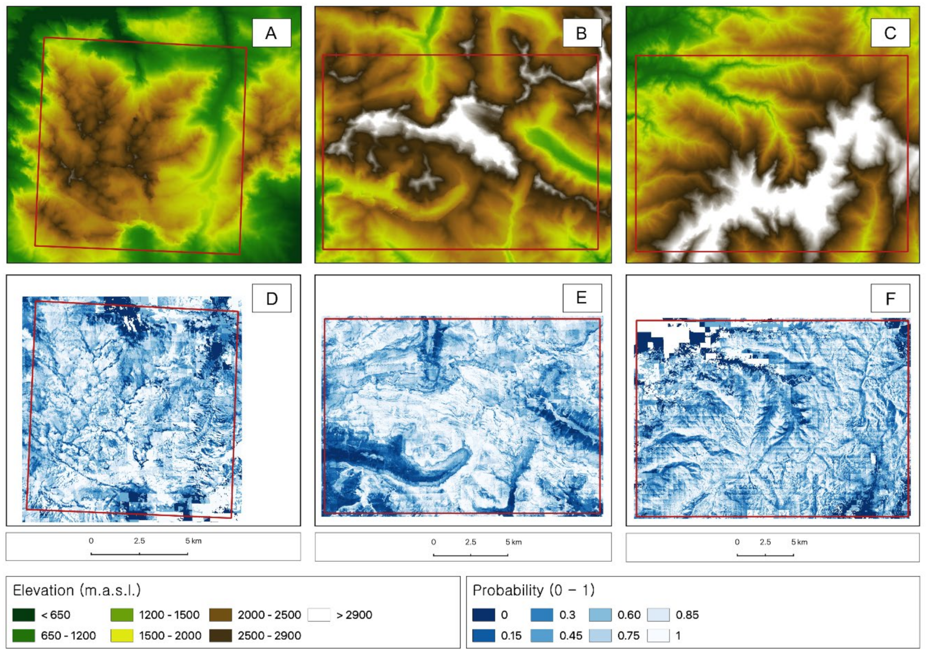
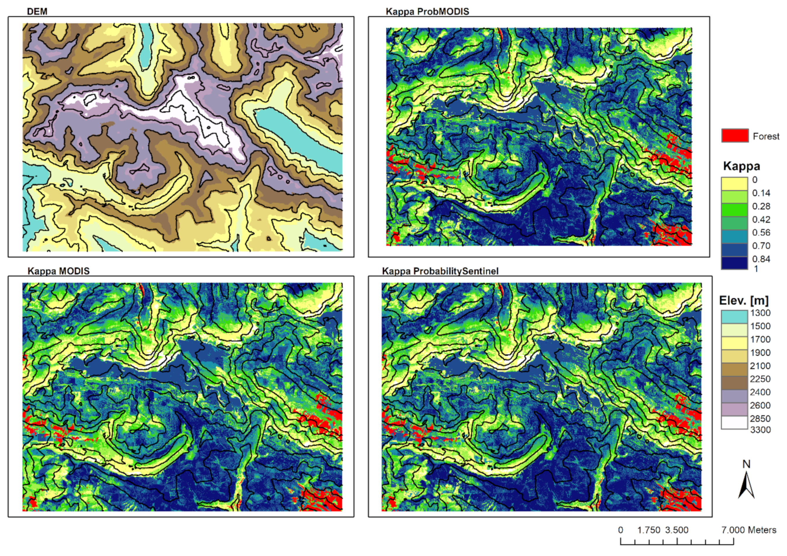
3.3. Spatial Impact When Mapping the Snow-Covered Area Distribution

The improvement of the methods was also been assessed spatially. In this way, for each test area both the Kappa coefficient and the percentage of agreement were computed inside each 20 m pixel including all dates with valid information (cloud-free days). In the three sites, ProbMODIS and ProbSentinel yielded more reliable snow-cover maps than those obtained with BinMODIS20m. In the Pyrenees (Figure 8), improved results were obtained with the two methodologies when compared to the Kappa coefficients of the BinMODIS20m maps. ProbMODIS has a better performance than ProbSentinel in the valleys but also in the higher areas. Nonetheless this improvement is minor, and the results were similar for almost the entire area. Figure 8 also shows a major shortcoming of MODIS snow retrieval which was not amended with any of the methods proposed. Snow distribution monitoring on steep slopes with a northerly aspect fails. Thus, in north-facing areas of deep valleys and in steep cirques with a northerly aspect, very low Kappa coefficients were obtained.
Results obtained for Picos de Europa (Figure S1 in the Supplementary Materials) also show a remarkable improvement when comparing the two probabilistic procedures to increase the spatial resolution of snow-cover mapping. The spatial distribution of the Kappa coefficients is again better for ProbMODIS, but ProbSentinel also improves BinMODIS20m. Again, north-facing areas show the inability of the MODIS sensor to retrieve snow-cover distribution. In Sierra Nevada (Figure S2), the spatial distribution of the Kappa coefficients renders equivalent conclusions to those obtained in the other test areas.
Another evaluation of the methods proposed here is to compute the daily fraction of original MODIS pixels (500 m resolution) having better, same, or worse results with the snow occurrence probabilities (ProbMODIS or ProbSentinel) when compared to BinMODIS20m. For all dates, the snow-cover mapping obtains better results (not shown) for a large fraction of the 500 m MODIS pixels, with no occurrence of worse performance for any date. This shows that ProbMODIS and ProbSentinel are better able to capture the snow-cover area distribution than MODIS observations directly downscaled, with superior results obtained with the ProbMODIS method.

3.4. Impact on Total Snow-Covered Area Estimation

Figure 9 depicts the frequency distribution of the absolute snow-covered area between Sentinel-2, the two probabilistic methods and BinMODIS20m. Overall, the ProbMODIS and ProbSentinel distributions are displaced towards lower errors, showing almost identical results. Nonetheless the mean improvement (vertical dashed lines in Figure 9) when mapping the total snow-covered area remains marginal.

4. Discussion

The spatial downscaling of MODIS snow products described here firstly accepted that a universal equation to transform the NDSI to FSC (Equation (2) [61]) is able to provide a good estimation of the snow-covered fraction inside MODIS pixel. Probably, other equations used to transform NDSI values to FSC [61,70], or specifically trained on each test site [71], would yield a more accurate representation of the snow-covered area inside each 500 m MODIS pixel. Nonetheless these would be empirical relations that need specific sensitivity tests to determine the thresholds better capturing the FSC classification. The universal NDSI-to-FSC transformation used here, together with the sensitivity tests for each site, provides a suitable classification of the MODIS retrieved snow-covered fraction, which in turn allows exploitation of the snow occurrence probability products.
The FSC threshold selection was based on the best mean value obtained in the sensitivity tests. These tests showed minor differences for close values around the selected thresholds (FSCthreshold ± 0.1 shows nearly equivalent performance), suggesting that the results may be impacted by small differences when selecting them [24].
For the vast majority of days during the study period, the snow occurrence distribution was better captured using the two probabilistic approaches as better Kappa values were obtained. As the snow season advanced, the improvement was more pronounced. Conversely, in the early snow season, the methodology failed more frequently. This result is related to the topographic control of snow distribution but also to the hysteresis behavior of snow dynamics [72,73]. This is an important drawback for the application of ProbMODIS and ProbSentinel, as the methodology has a lower confidence for observing the snow distribution for the initial snow accumulation events of the season. The snow distribution at the end of the snow season is highly impacted by both processes governing the snow accumulation and processes controlling melting dynamics [51,74], which are summed up as the snow season advances. Thus, at the end of the snow season the snow distribution shows repeated patterns [49,75,76], which allows improved results to be obtained compared with days early in the snow season. Such an outcome of the methodology shows that the main hypothesis accepted here, the snow distribution is strongly controlled by the topographic characteristics and this control has a high interannual persistence, has a stronger validity as the snow season advances. Hereby, it is shown that both, ProbMODIS and ProbSentinel snow occurrence probabilities take advantage of the topographic control of snow distribution [50,52,53,77] to downscale MODIS snow observations.
Spatially, the largest improvement of the probabilistic snow occurrence is obtained in lower-elevation areas, and zones with repeated accumulation and ablation cycles during the year. This highlights one of the major ameliorations of the methodology proposed here: improved understanding of snow-cover evolution processes in those areas having a discontinuous and more dynamic snow presence. Higher areas, with longer snow presence, also show better results with ProbMODIS and ProbSentinel when compared to BinMODIS20m. Nonetheless this improvement is minor as snow is present for longer periods as observed in high-elevation zones. This is evident in the Pyrenees above 1800–2000 m a.s.l., which is considered the elevation from which seasonal snow cover is observed [78]. In contrast, the moderate elevation of Picos de Europa or the melting events that can be expected even at the higher elevations of Sierra Nevada [58], causing a snow cover behavior transition above 2700 m [79,80], means that in these sites the improvement in high-elevation areas is also remarkable. One drawback of MODIS snow-cover retrieval, which is transferred to the final product of the probabilistic spatial resolution increase, is the deficient snow observation in very steep north-facing areas as these are affected by the amount of radiation received by a pixel [44,81].
As the Sentinel-2 mission has been available since late 2015 and the revisit time is 5 days, the evaluation of the methodology described here for days without clouds (or with minor cloud extent) would have led to very few evaluation dates [82]. To avoid this limitation, the evaluation strategy is focused on obtaining the bias estimates in cloud-free areas for both acquisitions, MODIS and Sentinel-2, with a 90% threshold of the cloud-covered area intersection. For some dates, this may have an impacted on the evaluation, as the cloud-free area may be in areas that are completely snow-covered or without snow presence. Moreover, clouds’ occurrence in mountain areas is highly impacted by the interaction between rugged terrain and the dominant wind direction [83], producing cloud patterns connected with the study area’s topography [84]. This irregular occurrence of clouds may have impacted the spatial evaluation of the probabilistic snow-mapping products, as some locations may have a much longer track record than others. Limitations from both cloud-cover occurrence and dissimilar lengths of snow occurrence in different zones of the study areas will become less important as Theia Sentinel-2 imagery continues to acquire images. Longer observation datasets will allow more reliable probabilities of snow occurrence to be generated, as more cases will be included in the training. For instance, Sentinel-2 pixels with the same Prob20m values which now are sorted by elevation would be rarer as more snow seasons are available. Thus, it is expected that as long as the Sentinel-2 mission continues to acquire observations, the snow occurrence probabilities will continue to improve their robustness, making the elevation sorting of pixels with the same probability unnecessary.
Overall, the snow distribution observations obtained with the methodology described here are limited by the inherent limitations of optical satellite sensor limitations [17,85]. Hereby, the observation of snow distribution in forested areas or restrictions derived from cloud cover presence are shortcomings that will be intrinsic to the observations derived from this spatial downscaling.
Of the two methods described and evaluated, ProbMODIS showed better results than ProbSentinel. Nonetheless, this difference is minor when compared with the improvement obtained from BinMODIS20m. This shows that accounting for the snow occurrence inside the 500 m MODIS pixels (as ProbMODIS does) is more precise than accounting for the snow occurrence in Sentinel-2 pixels independently of each other. Thus, use of the ProbMODIS algorithm is recommended to retrieve the snow probability occurrence and then binarize the FSC should be binarized according to the thresholds of the sensitivity tests performed.
The probabilistic snow occurrence approach described here is only able to improve the snow-mapping resolution in partially snow-covered MODIS pixels. Because not all pixels, and sometimes a minor fraction of them, are partially snow-covered (when compared to the entire snow-covered area), neither method has a major impact in quantifying the total snow-covered area. This lesser extent of partially snow-covered pixels also explains the fact that for the vast majority of days, similar results were obtained for a larger portion of the 500 m MODIS. However, the improvement obtained in transition zones can have remarkable importance for monitoring snow hydrology as snow-dominated zones lead to rain-dominated zones [86].
Other spatial downscaling methods of MODIS snow-cover products have also provided reliable and accurate snow maps [45], with even higher spatial resolution than that obtained in this study [47]. These authors were able to downscale MODIS snow-cover information to very high spatial resolution (3 m) with very good results. Nonetheless this latter method required both a Digital Elevation Model (DEM) and a training/validation dataset with the same spatial resolution as that of the final product, and a specific sensitivity test to determine the weights of the terrain parameters and their search distances. The main benefits of the method proposed here when compared to previous works [44], [45,47], is that it only relies on space borne satellite observations of the snow cover without any further requirement on the computation of the spectral reflectance or the calculation of further topographic variables. Hereby, as the spatial downscaling of MODIS snow cover observations with ProbMODIS and ProbSentinel, is rather simple and moreover it exploits already available snow cover observations (Theia snow collection and the NDSI from the NASA Earth Observation database), it has an easy and straight forward use. As the methodology obtains reliable and accurate snow cover patterns its simplicity and low computational requirements are the main benefits of its use.
Although the methodology presented requires probabilistic training with the already available database of Sentinel-2 observations, the approach is suitable for a wide variety of applications requiring high spatial resolution information on snow occurrence before the Sentinel-2 mission started. For instance, studies aiming to understand the ecological cycles of mountain pastures require detailed observations of snow disappearance over a longer time period [4,87]. Similarly, soil erosion in steep mountain areas is tightly related to snow gliding phenomena [7], which may occur at slope scales but also at landscape scales [88] and thus can also benefit from long-lasting and high spatial resolution snow-cover observations. The authors of [30] described and exploited a Snow Persistence index to determine long-lasting snow-covered areas (due to wind redistribution and avalanche action) and evaluate snow redistribution models. This latter index was derived from Sentinel-2 and Landsat-8 imagery, in the same way that ProbSentinel probability was computed here, showing that the spatial downscaling of MODIS snow cover observations is valuable for evaluation of high spatial resolution snow cover models. Another research topic that would also take advantage of high spatial resolution snow maps is the monitoring of very small glaciers [89], as these observations would allow an understanding of glacier dynamics in areas under threat from climate change [90]. Another subject that can benefit from this MODIS spatial downscaling is the study of the habitat of some animal species, as snow affects the distribution of forage species [91]. Lastly, the seasonal snow cover at low elevations in temperate mountain regions is predicted to cause important snowpack changes [92]. This demonstrates the importance of high spatial resolution snow monitoring with a long-lasting database [40] as this would allow changes occurring in mountain areas to be understood.

5. Conclusions

The methodology detailed here demonstrated that it is possible to spatially downscale MODIS snow cover observations by simply determining the snow occurrence probability from a database of higher spatial resolution, in this case study Theia snow distribution maps from Sentinel-2. The amelioration of the snow cover mapping is based on the strong topographic control of the snow distribution that characterizes mountain areas. Using several snow seasons to generate a snow occurrence probability for the original 500 m MODIS pixels (ProbMODIS) or an entire Sentinel-2 tile (ProbSentinel), the methodology is able to improve the snow cover mapping in partially snow-covered MODIS pixels generating snow occurrence maps at a 20 m spatial resolution. Nonetheless the snow occurrence probability computed for each MODIS pixel obtained more reliable snow cover maps and is thus recommended. With the already available Sentinel-2 imagery it is possible to train snow probability occurrences for particular test areas, which after finding the FSC thresholds to classify snow pixels (snow-free, snow-covered or partially snow-covered) allows the generation of snow distribution maps at 20 m resolution from MODIS observations. Nonetheless, these snow observations may be impacted by the inherent limitations of optical satellite retrievals, and will have a lower confidence on the observed snow distribution in the early snow season. The simple computation of this method allows an easy application for a wide variety of research topics requiring a long-lasting database of high spatiotemporal resolution observations of snow distribution in mountain areas. Future work aims to derive ProbMODIS probabilities over the Iberian Peninsula mountain areas and then obtain a high spatial resolution database of snow distribution which may be of interest in other disciplines.

Supplementary Materials

The following are available online at https://0-www-mdpi-com.brum.beds.ac.uk/article/10.3390/rs13224513/s1, Figure S1. Spatial distribution of Kappa coefficients obtained in Picos de Europa for the BinMODIS20m (bottom left panel), ProbMODIS (upper right panel) and ProbSentinel (bottom right panel) methods. In the upper left panel, the DEM of this test area is included for easier interpretation of the results. Forested areas are masked in red. Figure S2. Spatial distribution of Kappa coefficients obtained in Sierra Nevada for the BinMODIS20m (bottom left panel), ProbMODIS (upper right panel) and ProbSentinel (bottom right panel) methods. In the upper left panel, the DEM of this test area is included for easier interpretation of the results. Forested areas are masked in red.

Author Contributions

Conceptualization, J.R., J.I.L.-M., S.G., E.A.-G. and G.R.-L.; methodology, J.R., G.R.-L.; software, E.A.-G., G.R.-L. and J.R.; validation, J.R.; formal analysis, J.R., G.R.-L.; investigation, J.I.L.-M.; resources, J.I.L.-M.; data curation, J.R.; writing—original draft preparation, J.R.; writing—review and editing, J.R., J.I.L.-M., S.G., E.A.-G. and G.R.-L.; visualization, J.R.; supervision, S.G., J.I.L.-M.; project administration, J.I.L.-M., J.R.; funding acquisition, J.R., J.I.L.-M. All authors have read and agreed to the published version of the manuscript.

Funding

This research was funded by HIDROIBERNIEVE: CGL2017-82216-R, the Grant Juan de la Cierva Incorporación IJC2018-036260-I of the Spanish Ministry of Science and Innovation, the ANR TOP project, grant ANR-20-CE32-0002 of the French Agence Nationale de la Recherche.

Data Availability Statement

Theia snow collection is available here: https://theia.cnes.fr/atdistrib/rocket/#/search?collection=Snow and MOIDS images were directly downloaded from https://worldview.earthdata.nasa.gov/ ProbMODIS routines can be found here: https://github.com/ealonsogzl/ProbModis (accessed on 10 October 2021).

Acknowledgments

This work was supported by the Spanish Ministry of Economy and Competitiveness project “HIDROIBERNIEVE: CGL2017-82216-R”, and the “Organismo autónomo de Parques Nacionales” with the project “Cartografía de alta resolución especial del manto de nieve y su variabilidad reciente en los PPNN de montaña y los impactos del cambio climático para el horizonte 2050”. J. Revuelto is supported by the Grant IJC2018-036260-I. S. Gascoin is supported by the ANR TOP project. The authors thanks the three anonymous reviewers and Norah Wang who edited this article.

Conflicts of Interest

The authors declare no conflict of interest.

Appendix A. Probability Assessment on ProbMODIS Product

ProbMODIS probabilities may also be interpreted as the probability of a Sentinel-2 pixel being snow-covered divided by the probability of a MODIS pixel being partially snow-covered. This interpretation can be justified with the Bayes theorem as follow. Let us assume that P(S2) is the probability of an S2 pixel being snow-covered (number of times in which snow is observed divided by the number of times there is an observation without clouds) and P(M) is the probability of a 20 m MODIS pixel being partially snow-covered (nearest-neighbor downscaling). ProbMODIS is defined as the number of times that a Sentinel-2 pixel is snow-covered divided by the total number of times that the entire MODIS pixel is partially snow-covered. This ProbMODIS can be expressed as
P r o b M O D I S = P ( S 2 | M )
This equation can be expressed as follows according to the Bayes theorem:
P r o b M O D I S = P ( M | S 2 )   P S 2 P M
Although for a nearly negligible fraction of snow-covered Sentinel-2 pixels, there are some occurrences of MODIS pixels with a FSC of 0, it can be assumed that
P ( M | S 2 ) = 1
The MODIS-Sentinel-2 observation discrepancies show that in some rare cases there can be acquisition errors, as there is snow observed with Sentinel-2 that is not observed with MODIS for the same day under clear-sky conditions. Assuming the truth of Equation (3), ProbMODIS can also be interpreted as:
P r o b M O D I S = P S 2 P M
Equation (4) shows that justifies the probability of a Sentinel-2 pixel being snow-covered divided by the probability of a MODIS pixel being partially snow-covered can also define ProbMODIS.

References

  1. Pomeroy, J.; Essery, R.; Toth, B. Implications of spatial distributions of snow mass and melt rate for snow-cover depletion: Observations in a subarctic mountain catchment. Ann. Glaciol. 2004, 38, 195–201. [Google Scholar] [CrossRef] [Green Version]
  2. Sproles, E.A.; Nolin, A.W.; Rittger, K.; Painter, T.H. Climate change impacts on maritime mountain snowpack in the Oregon Cascades. Hydrol. Earth Syst. Sci. 2013, 17, 2581–2597. [Google Scholar] [CrossRef] [Green Version]
  3. Viviroli, D.; Dürr, H.H.; Messerli, B.; Meybeck, M.; Weingartner, R. Mountains of the world, water towers for humanity: Typology, mapping, and global significance. Water Resour. Res. 2007, 43. [Google Scholar] [CrossRef] [Green Version]
  4. Carlson, B.Z.; Corona, M.C.; Dentant, C.; Bonet, R.; Thuiller, W.; Choler, P. Observed long-term greening of alpine vegetation—A case study in the French Alps. Environ. Res. Lett. 2017, 12, 114006. [Google Scholar] [CrossRef]
  5. Inouye, D.W.; McKinney, A.M. Phenological and ecological consequences of changes in winter snowpack in the Colorado Rocky Mountains. AGU Fall Meet. Abstr. 2012, 2012, B21I-05. [Google Scholar]
  6. Sanmiguel-Vallelado, A.; Camarero, J.J.; Gazol, A.; Morán-Tejeda, E.; Sangüesa-Barreda, G.; Alonso-González, E.; Gutiérrez, E.; Alla, A.Q.; Galván, J.D.; López-Moreno, J.I. Detecting snow-related signals in radial growth of Pinus uncinata mountain forests. Dendrochronologia 2019, 57, 125622. [Google Scholar] [CrossRef]
  7. Meusburger, K.; Leitinger, G.; Mabit, L.; Mueller, M.H.; Walter, A.; Alewell, C. Soil erosion by snow gliding—A first quantification attempt in a subalpine area in Switzerland. Hydrol. Earth Syst. Sci. 2014, 18, 3763–3775. [Google Scholar] [CrossRef] [Green Version]
  8. Fischer, M.; Huss, M.; Hoelzle, M. Surface elevation and mass changes of all Swiss glaciers 1980–2010. Cryosphere 2015, 9, 525–540. [Google Scholar] [CrossRef] [Green Version]
  9. Réveillet, M.; Vincent, C.; Six, D.; Rabatel, A. Which empirical model is best suited to simulate glacier mass balances? J. Glaciol. 2016, 63, 39–54. [Google Scholar] [CrossRef] [Green Version]
  10. Box, J.E.; Fettweis, X.; Stroeve, J.C.; Tedesco, M.; Hall, D.K.; Steffen, K. Greenland ice sheet albedo feedback: Thermodynamics and atmospheric drivers. Cryosphere 2012, 6, 821–839. [Google Scholar] [CrossRef] [Green Version]
  11. Hall, A. The Role of Surface Albedo Feedback in Climate. J. Climate 2004, 17, 1550–1568. [Google Scholar] [CrossRef] [Green Version]
  12. Dozier, J. Spectral signature of alpine snow cover from the landsat thematic mapper. Remote Sens. Environ. 1989, 28, 9–22. [Google Scholar] [CrossRef]
  13. Parajka, J.; Blöschl, G. Spatio-temporal combination of MODIS images—Potential for snow cover mapping. Water Resour. Res. 2008, 44. [Google Scholar] [CrossRef]
  14. Rosenthal, W.; Dozier, J. Automated Mapping of Montane Snow Cover at Subpixel Resolution from the Landsat Thematic Mapper. Water Resour. Res. 1996, 32, 115–130. [Google Scholar] [CrossRef]
  15. Hall, D.K.; Riggs, G.A.; Salomonson, V.V. Development of methods for mapping global snow cover using moderate resolution imaging spectroradiometer data. Remote Sens. Environ. 1995, 54, 127–140. [Google Scholar] [CrossRef]
  16. Liu, Y.; Chen, X.; Hao, J.-S.; Li, L. Snow cover estimation from MODIS and Sentinel-1 SAR data using machine learning algorithms in the western part of the Tianshan Mountains. J. Mt. Sci. 2020, 17, 884–897. [Google Scholar] [CrossRef]
  17. Masson, T.; Dumont, M.; Mura, M.D.; Sirguey, P.; Gascoin, S.; Dedieu, J.-P.; Chanussot, J. An Assessment of Existing Methodologies to Retrieve Snow Cover Fraction from MODIS Data. Remote Sens. 2018, 10, 619. [Google Scholar] [CrossRef] [Green Version]
  18. Gascoin, S.; Grizonnet, M.; Bouchet, M.; Salgues, G.; Hagolle, O. Theia Snow collection: High-resolution operational snow cover maps from Sentinel-2 and Landsat-8 data. Earth Syst. Sci. Data 2019, 11, 493–514. [Google Scholar] [CrossRef] [Green Version]
  19. Hall, D.K.; Riggs, G.A.; DiGirolamo, N.E.; Román, M.O. Evaluation of MODIS and VIIRS cloud-gap-filled snow-cover products for production of an Earth science data record. Hydrol. Earth Syst. Sci. 2019, 23, 5227–5241. [Google Scholar] [CrossRef] [Green Version]
  20. Klein, A.G.; Barnett, A.C. Validation of daily MODIS snow cover maps of the Upper Rio Grande River Basin for the 2000–2001 snow year. emote. Sens. Environ. 2003, 86, 162–176. [Google Scholar] [CrossRef]
  21. Dietz, A.; Kuenzer, C.; Gessner, U.; Dech, S. Remote sensing of snow—A review of available methods. Int. J. Remote Sens. 2011, 33, 4094–4134. [Google Scholar] [CrossRef]
  22. Hall, D.K.; Riggs, G.A.; Salomonson, V.V.; DiGirolamo, N.E.; Bayr, K.J. MODIS snow-cover products. Remote Sens. Environ. 2002, 83, 181–194. [Google Scholar] [CrossRef] [Green Version]
  23. Riggs, G.A.; Hall, D.K.; Román, M.O. Overview of NASA’s MODIS and Visible Infrared Imaging Radiometer Suite (VIIRS) snow-cover Earth System Data Records. Earth Syst. Sci. Data 2017, 9, 765–777. [Google Scholar] [CrossRef] [Green Version]
  24. Gascoin, S.; Hagolle, O.; Huc, M.; Jarlan, L.; Dejoux, J.-F.; Szczypta, C.; Marti, R.; Sánchez, R. A snow cover climatology for the Pyrenees from MODIS snow products. Hydrol. Earth Syst. Sci. 2015, 19, 2337–2351. [Google Scholar] [CrossRef] [Green Version]
  25. Paudel, K.P.; Andersen, P. Monitoring snow cover variability in an agropastoral area in the Trans Himalayan region of Nepal using MODIS data with improved cloud removal methodology. Remote Sens. Environ. 2011, 115, 1234–1246. [Google Scholar] [CrossRef]
  26. Saavedra, F.A.; Kampf, S.K.; Fassnacht, S.R.; Sibold, J.S. A snow climatology of the Andes Mountains from MODIS snow cover data. Int. J. Clim. 2016, 37, 1526–1539. [Google Scholar] [CrossRef]
  27. Blöschl, G. Scaling issues in snow hydrology. Hydrol. Process. 1999, 13, 2149–2175. [Google Scholar] [CrossRef]
  28. Deems, J.S.; Fassnacht, S.R.; Elder, K.J. Fractal Distribution of Snow Depth from Lidar Data. J. Hydrometeorol. 2006, 7, 285–297. [Google Scholar] [CrossRef]
  29. Mendoza, P.A.; Musselman, K.N.; Revuelto, J.; Deems, J.S.; López-Moreno, J.I.; McPhee, J. Interannual and Seasonal Variability of Snow Depth Scaling Behavior in a Subalpine Catchment. Water Resour. Res. 2020, 56, e2020WR02. [Google Scholar] [CrossRef]
  30. Wayand, N.E.; Marsh, C.B.; Shea, J.M.; Pomeroy, J.W. Globally scalable alpine snow metrics. Remote Sens. Environ. 2018, 213, 61–72. [Google Scholar] [CrossRef]
  31. Anderton, S.P.; White, S.M.; Alvera, B. Micro-scale spatial variability and the timing of snow melt runoff in a high mountain catchment. J. Hydrol. 2002, 268, 158–176. [Google Scholar] [CrossRef]
  32. Carlson, B.Z.; Choler, P.; Renaud, J.; Dedieu, J.-P.; Thuiller, W. Modelling snow cover duration improves predictions of functional and taxonomic diversity for alpine plant communities. Ann. Bot. 2015, 116, 1023–1034. [Google Scholar] [CrossRef] [PubMed] [Green Version]
  33. Clark, M.P.; Hendrikx, J.; Slater, A.; Kavetski, D.; Anderson, B.; Cullen, N.J.; Kerr, T.; Hreinsson, E.; Woods, R. Representing spatial variability of snow water equivalent in hydrologic and land-surface models: A review. Water Resour. Res. 2011, 47. [Google Scholar] [CrossRef] [Green Version]
  34. López-Moreno, J.I.; Stähli, M. Statistical analysis of the snow cover variability in a subalpine watershed: Assessing the role of topography and forest interactions. J. Hydrol. 2008, 348, 379–394. [Google Scholar] [CrossRef]
  35. Gascon, F.; Bouzinac, C.; Thépaut, O.; Jung, M.; Francesconi, B.; Louis, J.; Lonjou, V.; Lafrance, B.; Massera, S.; Gaudel-Vacaresse, A.; et al. Copernicus Sentinel-2A Calibration and Products Validation Status. Remote Sens. 2017, 9, 584. [Google Scholar] [CrossRef] [Green Version]
  36. Drusch, M.; Del Bello, U.; Carlier, S.; Colin, O.; Fernandez, V.; Gascon, F.; Hoersch, B.; Isola, C.; Laberinti, P.; Martimort, P.; et al. Sentinel-2: ESA’s Optical High-Resolution Mission for GMES Operational Services. Remote Sens. Environ. 2012, 120, 25–36. [Google Scholar] [CrossRef]
  37. Gascoin, S.; Grizonnet, M.; Klempka, T.; Salges, G. Algorithm theoretical basis documentation for an operational snow cover product from Sentinel-2 and Landsat-8 data (Let-it-snow). Zenodo 2018. [Google Scholar] [CrossRef]
  38. Baba, M.W.; Gascoin, S.; Hanich, L. Assimilation of Sentinel-2 Data into a Snowpack Model in the High Atlas of Morocco. Remote Sens. 2018, 10, 1982. [Google Scholar] [CrossRef] [Green Version]
  39. Dong, C.; Menzel, L. Producing cloud-free MODIS snow cover products with conditional probability interpolation and meteorological data. Remote Sens. Environ. 2016, 186, 439–451. [Google Scholar] [CrossRef]
  40. Bormann, K.J.; Brown, R.D.; Derksen, C.; Painter, T.H. Estimating snow-cover trends from space. Nat. Clim. Chang. 2018, 8, 924–928. [Google Scholar] [CrossRef]
  41. Dozier, J.; Bair, E.H.; Davis, R.E. Estimating the spatial distribution of snow water equivalent in the world’s mountains. Wiley Interdiscip. Rev. Water 2016, 3, 461–474. [Google Scholar] [CrossRef]
  42. Atkinson, P.M. Downscaling in remote sensing. Int. J. Appl. Earth Obs. Geoinf. 2013, 22, 106–114. [Google Scholar] [CrossRef]
  43. Peng, J.; Loew, A.; Merlin, O.; Verhoest, N.E.C. A review of spatial downscaling of satellite remotely sensed soil moisture. Rev. Geophys. 2017, 55, 341–366. [Google Scholar] [CrossRef]
  44. Sirguey, P.; Mathieu, R.; Arnaud, Y. Subpixel monitoring of the seasonal snow cover with MODIS at 250 m spatial resolution in the Southern Alps of New Zealand: Methodology and accuracy assessment. Remote Sens. Environ. 2009, 113, 160–181. [Google Scholar] [CrossRef]
  45. Berman, E.E.; Bolton, D.K.; Coops, N.C.; Mityok, Z.K.; Stenhouse, G.B.; Moore, R.D. Daily estimates of Landsat fractional snow cover driven by MODIS and dynamic time-warping. Remote Sens. Environ. 2018, 216, 635–646. [Google Scholar] [CrossRef]
  46. Durand, M.; Molotch, N.P.; Margulis, S.A. Merging complementary remote sensing datasets in the context of snow water equivalent reconstruction. Remote Sens. Environ. 2008, 112, 1212–1225. [Google Scholar] [CrossRef]
  47. Cristea, N.C.; Breckheimer, I.; Raleigh, M.S.; HilleRisLambers, J.; Lundquist, J.D. An evaluation of terrain-based downscaling of fractional snow covered area data sets based on LiDAR-derived snow data and orthoimagery. Water Resour. Res. 2017, 53, 6802–6820. [Google Scholar] [CrossRef]
  48. Golding, D.L.; Swanson, R.H. Snow distribution patterns in clearings and adjacent forest. Water Resour. Res. 1986, 22, 1931–1940. [Google Scholar] [CrossRef] [Green Version]
  49. Sturm, M.; Wagner, A.M. Using repeated patterns in snow distribution modeling: An Arctic example. Water Resour. Res. 2010, 46. [Google Scholar] [CrossRef] [Green Version]
  50. Erickson, T.A.; Williams, M.W.; Winstral, A. Persistence of topographic controls on the spatial distribution of snow in rugged mountain terrain, Colorado, United States. Water Resour. Res. 2005, 41, 1–17. [Google Scholar] [CrossRef] [Green Version]
  51. Jost, G.; Weiler, M.; Gluns, D.R.; Alila, Y. The influence of forest and topography on snow accumulation and melt at the watershed-scale. J. Hydrol. 2007, 347, 101–115. [Google Scholar] [CrossRef]
  52. Revuelto, J.; López-Moreno, J.I.; Azorin-Molina, C.; Vicente-Serrano, S.M. Topographic control of snowpack distribution in a small catchment in the central Spanish Pyrenees: Intra- and inter-annual persistence. Cryosphere 2014, 8, 1989–2006. [Google Scholar] [CrossRef] [Green Version]
  53. Schirmer, M.; Wirz, V.; Clifton, A.; Lehning, M. Persistence in intra-annual snow depth distribution: 1.Measurements and topographic control. Water Resour. Res. 2011, 47, W09516. [Google Scholar] [CrossRef] [Green Version]
  54. García-Ruiz, J.M.G.; Martí-Bono, C.E.M. Mapa Geomorfológico del Parque Nacional de Ordesa y Monte Perdido. 2001. Available online: https://dialnet.unirioja.es/servlet/libro?codigo=122546 (accessed on 7 June 2021).
  55. García-Ruiz, J.M.; Palacios, D.; de Andrés, N.; Valero-Garcés, B.L.; López-Moreno, J.I.; Sanjuán, Y. Holocene and “Little Ice Age” glacial activity in the Marboré Cirque, Monte Perdido Massif, Central Spanish Pyrenees. Holocene 2014, 24, 1439–1452. [Google Scholar] [CrossRef] [Green Version]
  56. López-Moreno, J.I.; Vicente-Serrano, S.M. Atmospheric circulation influence on the interannual variability of snow pack in the Spanish Pyrenees during the second half of the 20th century. Hydrol. Res. 2007, 38, 33–44. [Google Scholar] [CrossRef] [Green Version]
  57. López-Moreno, J.I.; Nogués-Bravo, D. Interpolating local snow depth data: An evaluation of methods. Hydrol. Process. 2006, 20, 2217–2232. [Google Scholar] [CrossRef]
  58. Herrero, J.; Polo, M.J. Evaposublimation from the snow in the Mediterranean mountains of Sierra Nevada (Spain). Cryosphere 2016, 10, 2981–2998. [Google Scholar] [CrossRef] [Green Version]
  59. Ruiz-Fernández, J.; Oliva, M.; Hrbáček, F.; Vieira, G.; García-Hernández, C. Soil temperatures in an Atlantic high mountain environment: The Forcadona buried ice patch (Picos de Europa, NW Spain). CATENA 2017, 149, 637–647. [Google Scholar] [CrossRef]
  60. Riggs, G.A.; Hall, D.K.; Román, M.O. MODIS Snow Products User Guide for Collection 6.1 (C6.1). Available online: https://modis-snow-ice.gsfc.nasa.gov/?c=userguides (accessed on 15 June 2021).
  61. Salomonson, V.V.; Appel, I. Estimating fractional snow cover from MODIS using the normalized difference snow index. Remote Sens. Environ. 2004, 89, 351–360. [Google Scholar] [CrossRef]
  62. Cohen, J. A Coefficient of Agreement for Nominal Scales. Educ. Psychol. Meas. 1960, 20, 37–46. [Google Scholar] [CrossRef]
  63. Foody, G.M. Thematic Map Comparison. Photogramm. Eng. Remote Sens. 2004, 70, 627–633. [Google Scholar] [CrossRef]
  64. Liu, C.; Frazier, P.; Kumar, L. Comparative assessment of the measures of thematic classification accuracy. Remote Sens. Environ. 2007, 107, 606–616. [Google Scholar] [CrossRef]
  65. Stehman, S.V. Selecting and interpreting measures of thematic classification accuracy. Remote Sens. Environ. 1997, 62, 77–89. [Google Scholar] [CrossRef]
  66. Wilkinson, G.G. Results and implications of a study of fifteen years of satellite image classification experiments. IEEE Trans. Geosci. Remote Sens. 2005, 43, 433–440. [Google Scholar] [CrossRef]
  67. Morales-Barquero, L.; Lyons, M.B.; Phinn, S.R.; Roelfsema, C.M. Trends in Remote Sensing Accuracy Assessment Approaches in the Context of Natural Resources. Remote Sens. 2019, 11, 2305. [Google Scholar] [CrossRef] [Green Version]
  68. Stehman, S.V. Estimating the kappa coefficient and its variance under stratified random sampling. Photogramm. Eng. Remote Sens. 1996, 62, 401–407. [Google Scholar]
  69. Brovelli, M.A.; Crespi, M.; Fratarcangeli, F.; Giannone, F.; Realini, E. Accuracy assessment of high resolution satellite imagery orientation by leave-one-out method. ISPRS J. Photogramm. Remote Sens. 2008, 63, 427–440. [Google Scholar] [CrossRef]
  70. Rittger, K.; Painter, T.H.; Dozier, J. Assessment of methods for mapping snow cover from MODIS. Adv. Water Resour. 2013, 51, 367–380. [Google Scholar] [CrossRef]
  71. Alonso-González, E.; Gutmann, E.; Aalstad, K.; Fayad, A.; Bouchet, M.; Gascoin, S. Snowpack dynamics in the Lebanese mountains from quasi-dynamically downscaled ERA5 reanalysis updated by assimilating remotely sensed fractional snow-covered area. Hydrol. Earth Syst. Sci. 2021, 25, 4455–4471. [Google Scholar] [CrossRef]
  72. Egli, L.; Jonas, T. Hysteretic dynamics of seasonal snow depth distribution in the Swiss Alps. Geophys. Res. Lett. 2009, 36, L02501. [Google Scholar] [CrossRef] [Green Version]
  73. Magand, C.; Ducharne, A.; Moine, N.L.; Gascoin, S. Introducing Hysteresis in Snow Depletion Curves to Improve the Water Budget of a Land Surface Model in an Alpine Catchment. J. Hydrometeorol. 2014, 15, 631–649. [Google Scholar] [CrossRef] [Green Version]
  74. DeBeer, C.M.; Pomeroy, J.W. Modelling snow melt and snowcover depletion in a small alpine cirque, Canadian Rocky Mountains. Hydrol. Process. 2009, 23, 2584–2599. [Google Scholar] [CrossRef]
  75. Helfricht, K.; Schöber, J.; Schneider, K.; Sailer, R.; Kuhn, M. Interannual persistence of the seasonal snow cover in a glacierized catchment. J. Glaciol. 2014, 60, 889–904. [Google Scholar] [CrossRef] [Green Version]
  76. López-Moreno, J.I.; Revuelto, J.; González, E.A.; Sanmiguel-Vallelado, A.; Fassnacht, S.R.; Deems, J.; Morán-Tejeda, E. Using very long-range terrestrial laser scanner to analyze the temporal consistency of the snowpack distribution in a high mountain environment. J. Mt. Sci. 2017, 14, 823–842. [Google Scholar] [CrossRef]
  77. Trujillo, E.; Ramírez, J.A.; Elder, K.J. Topographic, meteorologic, and canopy controls on the scaling characteristics of the spatial distribution of snow depth fields. Water Resour. Res. 2007, 43, W07409. [Google Scholar] [CrossRef]
  78. López-Moreno, J.I.; Soubeyroux, J.M.; Gascoin, S.; Alonso-Gonzalez, E.; Durán-Gómez, N.; Lafaysse, M.; Vernay, M.; Carmagnola, C.; Morin, S. Long-term trends (1958–2017) in snow cover duration and depth in the Pyrenees. Int. J. Clim. 2020, 40, 6122–6136. [Google Scholar] [CrossRef]
  79. Alonso-González, E.; López-Moreno, J.I.; Navarro-Serrano, F.; Sanmiguel-Vallelado, A.; Revuelto, J.; Domínguez-Castro, F.; Ceballos, A. Snow climatology for the mountains in the Iberian Peninsula using satellite imagery and simulations with dynamically downscaled reanalysis data. Int. J. Clim. 2019, 40, 477–491. [Google Scholar] [CrossRef]
  80. Pimentel, R.; Herrero, J.; Polo, M. Quantifying Snow Cover Distribution in Semiarid Regions Combining Satellite and Terrestrial Imagery. Remote Sens. 2017, 9, 995. [Google Scholar] [CrossRef] [Green Version]
  81. Cluzet, B.; Lafaysse, M.; Cosme, E.; Albergel, C.; Meunier, L.-F.; Dumont, M. CrocO_v1.0: A particle filter to assimilate snowpack observations in a spatialised framework. Geosci. Model Dev. 2021, 14, 1595–1614. [Google Scholar] [CrossRef]
  82. Parajka, J.; Pepe, M.; Rampini, A.; Rossi, S.; Blöschl, G. A regional snow-line method for estimating snow cover from MODIS during cloud cover. J. Hydrol. 2010, 381, 203–212. [Google Scholar] [CrossRef]
  83. Banta, R.M. The Role of Mountain Flows in Making Clouds. In Atmospheric Processes Over Complex Terrain; Banta, R.M., Berri, G., Blumen, W., Carruthers, D.J., Dalu, G.A., Durran, D.R., Egger, J., Garratt, J.R., Hanna, S.R., Hunt, J.C.R., et al., Eds.; American Meteorological Society: Boston, MA, USA, 1990; pp. 229–283. [Google Scholar] [CrossRef]
  84. Parajka, J.; Blöschl, G. Validation of MODIS snow cover images over Austria. Hydrol. Earth Syst. Sci. 2006, 10, 679–689. [Google Scholar] [CrossRef] [Green Version]
  85. Largeron, C.; Dumont, M.; Morin, S.; Boone, A.; Lafaysse, M.; Metref, S.; Cosme, E.; Jonas, T.; Winstral, A.; Margulis, S.A. Toward Snow Cover Estimation in Mountainous Areas Using Modern Data Assimilation Methods: A Review. Front. Earth Sci. 2020, 8. [Google Scholar] [CrossRef]
  86. Fayad, A.; Gascoin, S.; Faour, G.; Lopez-Moreno, I.; Drapeau, L.; Le Page, M.; Escadafal, R. Snow hydrology in Mediterranean mountain regions: A review. J. Hydrol. 2017, 551, 374–396. [Google Scholar] [CrossRef]
  87. Dedieu, J.-P.; Carlson, B.Z.; Bigot, S.; Sirguey, P.; Vionnet, V.; Choler, P. On the Importance of High-Resolution Time Series of Optical Imagery for Quantifying the Effects of Snow Cover Duration on Alpine Plant Habitat. Remote Sens. 2016, 8, 481. [Google Scholar] [CrossRef] [Green Version]
  88. Leitinger, G.; Meusburger, K.; Rüdisser, J.; Tasser, E.; Walde, J.; Höller, P. Spatial evaluation of snow gliding in the Alps. CATENA 2018, 165, 567–575. [Google Scholar] [CrossRef]
  89. Huss, M.; Fischer, M. Sensitivity of Very Small Glaciers in the Swiss Alps to Future Climate Change. Front. Earth Sci. 2016, 4. [Google Scholar] [CrossRef] [Green Version]
  90. Beniston, M.; Farinotti, D.; Stoffel, M.; Andreassen, L.M.; Coppola, E.; Eckert, N.; Fantini, A.; Giacona, F.; Hauck, C.; Huss, M.; et al. The European mountain cryosphere: A review of its current state, trends, and future challenges. Cryosphere 2018, 12, 759–794. [Google Scholar] [CrossRef] [Green Version]
  91. Macander, M.J.; Swingley, C.S.; Joly, K.; Raynolds, M.K. Landsat-based snow persistence map for northwest Alaska. Remote Sens. Environ. 2015, 163, 23–31. [Google Scholar] [CrossRef]
  92. Adam, J.C.; Hamlet, A.F.; Lettenmaier, D.P. Implications of global climate change for snowmelt hydrology in the twenty-first century. Hydrol. Process. 2008, 23, 962–972. [Google Scholar] [CrossRef]
Figure 1. Digital Elevation Models (DEM) of the study areas, and location of these sites within the Iberian Peninsula DEMs from the Instituto Geográfico Nacional (Spanish National Geographic Institute).
Remotesensing 13 04513 g001
Figure 2. Overall flow chart of the methodology. Blue and green arrows indicate the information needed to derive ProbSentinel and ProbMODIS snow occurrence probabilities. Red arrows depict the observations needed to obtain the spatially downscaled snow distribution products.
Remotesensing 13 04513 g002
Figure 3. The (AC) panels respectively show the Digital Elevation Models (DEM) of Picos de Europa, the Pyrenees and Sierra Nevada (DEMs from the Instituto Geográfico Nacional (Spanish National Geographic Institute)). The (DF) panels depict the spatial distribution of the ProbMODIS probabilities for Picos de Europa, the Pyrenees and Sierra Nevada, respectively. The probabilities of this example were obtained for the entire study period with Sentinel-2 images (2015–2021).
Remotesensing 13 04513 g003
Figure 4. Mean value and standard deviation of the Kappa coefficients obtained in the sensitivity test of BinMODIS20m for the different FSC thresholds.
Remotesensing 13 04513 g004
Figure 5. The mean value and standard deviation of the Kappa coefficients obtained in the paired sensitivity test to determine the upper and lower FSC thresholds. The upper graph depicts the ProbMODIS sensitivity test, and the lower graph shows the ProbSentinel sensitivity test. The light green shaded area shows the results for the upper limit sensitivity tests, and the non-shaded area the results of the lower limit sensitivity test. These graphs include the results obtained in the three test areas.
Remotesensing 13 04513 g005
Figure 6. Kappa coefficient scatter plot of ProbMODIS (left panel graphs) and ProbSentinel (right panel graphs) versus the Kappa coefficients of BinMODIS20m. The color scale depicts the day of the snow season (Day Of Year starting October 1).
Remotesensing 13 04513 g006
Figure 7. Percentage of agreement scatter plot of ProbMODIS (left panel graphs) and ProbSentinel (right panel graphs) versus percentage of agreement of BinMODIS20m. The color scale depicts the day of the snow season (Day Of Year starting October 1).
Remotesensing 13 04513 g007
Figure 8. Spatial distribution of Kappa coefficients obtained in the Pyrenees for BinMODIS20m imagery (bottom left panel), ProbMODIS (upper right panel) and ProbSentinel (bottom right panel) methods. In the upper left panel, the DEM of this test area is included for easier interpretation of the results. Forested areas are masked in red.
Remotesensing 13 04513 g008
Figure 9. Frequency distribution of the absolute error in total snow-covered area estimation obtained for ProbMODIS (upper panel) and ProbSentinel (bottom panel) when compared to the snow-covered area retrieved with Sentinel-2. The two graphs also depict the BinMODIS20m frequency distribution. Vertical dashed lines show the corresponding mean snow-covered area error during the study period. These graphs include the results for the three sites.
Remotesensing 13 04513 g009
Table 1. FSC thresholds to classify the snow cover in the 500 m MODIS pixels. The snow occurrence probabilities are only used in the partially snow-covered pixels. The 20 m pixels inside the NoSnow MODIS pixels area are all assigned as snow-free, and for the AllSnow covered cases, all 20 m pixels are set as snow-covered.
Test AreaNo SnowPartially Snow-CoveredAll Snow
PyreneesFSC ≤ 0.250.25 < FSC ≤ 0.750.75 < FSC
Sierra NevadaFSC ≤ 0.150.15 < FSC ≤ 0.850.85 < FSC
Picos de EuropaFSC ≤ 0.150.15 < FSC ≤ 0.750.75 < FSC
Table 2. Mean values and standard deviations of the error estimates for the three study sites.
Study AreaMethodKappaAgree
MeanCVMeanCV
PyreneesProbMODIS0.570.2184.238.41
ProbSentinel0.550.2183.928.49
BinMODIS20m0.510.2382.768.94
Picos de EuropaProbMODIS0.520.2187.147.38
ProbSentinel0.510.2186.887.54
BinMODIS20m0.410.2585.068.64
Sierra NevadaProbMODIS0.710.1591.253.18
ProbSentinel0.70.1590.863.3
BinMODIS20m0.640.1889.314.04
Publisher’s Note: MDPI stays neutral with regard to jurisdictional claims in published maps and institutional affiliations.

