
Assessing the Impacts of Species Composition on the Accuracy of Mapping Chlorophyll Content in Heterogeneous Ecosystems


1
Department of Geography, Simon Fraser University, 8888 University Drive, Burnaby, BC V5A 1S6, Canada
2
Department of Geography, Geomatics and Environment, University of Toronto Mississauga, 3359 Mississauga Road, Mississauga, ON L5L 1C6, Canada
*
Author to whom correspondence should be addressed.
Remote Sens. 2021, 13(22), 4671; https://0-doi-org.brum.beds.ac.uk/10.3390/rs13224671
Submission received: 14 October 2021
/
Revised: 17 November 2021
/
Accepted: 17 November 2021
/
Published: 19 November 2021
(This article belongs to the Special Issue New Insights into Ecosystem Monitoring Using Geospatial Techniques)
Abstract
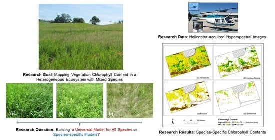
:Chlorophyll is an essential vegetation pigment influencing plant photosynthesis rate and growth conditions. Remote sensing images have been widely used for mapping vegetation chlorophyll content in different ecosystems (e.g., farmlands, forests, grasslands, and wetlands) for evaluating vegetation growth status and productivity of these ecosystems. Compared to farmlands and forests that are more homogeneous in terms of species composition, grasslands and wetlands are more heterogeneous with highly mixed species (e.g., various grass, forb, and shrub species). Different species contribute differently to the ecosystem services, thus, monitoring species-specific chlorophyll content is critical for better understanding their growth status, evaluating ecosystem functions, and supporting ecosystem management (e.g., control invasive species). However, previous studies in mapping chlorophyll content in heterogeneous ecosystems have rarely estimated species-specific chlorophyll content, which was partially due to the limited spatial resolution of remote sensing images commonly used in the past few decades for recognizing different species. In addition, many previous studies have used one universal model built with data of all species for mapping chlorophyll of the entire study area, which did not fully consider the impacts of species composition on the accuracy of chlorophyll estimation (i.e., establishing species-specific chlorophyll estimation models may generate higher accuracy). In this study, helicopter-acquired high-spatial resolution hyperspectral images were acquired for species classification and species-specific chlorophyll content estimation. Four estimation models, including a universal linear regression (LR) model (i.e., built with data of all species), species-specific LR models (i.e., built with data of each species, respectively), a universal random forest regression (RFR) model, and species-specific RFR models, were compared to determine their performance in mapping chlorophyll and to evaluate the impacts of species composition. The results show that species-specific models performed better than the universal models, especially for species with fewer samples in the dataset. The best performed species-specific models were then used to generate species-specific chlorophyll content maps using the species classification results. Impacts of species composition on the retrieval of chlorophyll content were further assessed to support future chlorophyll mapping in heterogeneous ecosystems and ecosystem management.
1. Introduction
Chlorophyll content is a critical vegetation feature that influences photosynthesis process and plant growth [1,2]. Therefore, mapping chlorophyll content is essential for understanding plant physiological conditions, evaluating ecosystem status, and supporting ecosystem management [3,4,5]. Chlorophyll contents can be measured at selected study sites in the field, which, however, is costly, labor-intensive, and lacks representativeness [6]. In contrast, remote sensing is an efficient and low-cost tool for mapping chlorophyll contents of the entire study area and monitoring its spatiotemporal variations [7,8].
Remote sensing images have been used in previous studies for mapping chlorophyll content in different ecosystems, such as farmlands [3,9,10,11], forests [12,13,14], grasslands [15,16,17], and wetlands [18,19]. Among these ecosystems, the farmlands and forests are more homogeneous in terms of species composition. In contrast, grasslands and wetlands are more heterogeneous with highly mixed species (e.g., different grass, forb, and shrub species). Various species provide food and habitat to different wildlife, contribute differently to ecosystem productivity and carbon cycling, and play different roles in other ecosystem services (e.g., negative impacts of invasive species). Therefore, mapping species-specific chlorophyll content is critical for better understanding ecosystem functions and developing corresponding ecosystem management strategies. Previous studies mapping chlorophyll content have focused more on landscape or regional scales and generated chlorophyll maps for understanding its spatial variations [9,20]. However, few have focused on species-level chlorophyll mapping and investigating variations of chlorophyll contents between species and how that affects ecosystem status. This is partially due to the limited spatial resolution of remote sensing images (e.g., 2.4 m of QuickBird imagery and 6 m of SPOT-7 imagery) for recognizing mixed species [15,21]. In this study, 30 cm-resolution hyperspectral images were acquired for classifying different species using an object-based approach and consequently for mapping species-specific chlorophyll content.
Data analytical models (e.g., linear regression (LR), random forest regression (RFR), or physically-based PROSAIL) are needed to estimate chlorophyll contents or other vegetation properties (e.g., biomass) using remote sensing data [17,22,23,24]. Typically, a universal model was used in each of the previous studies for estimating vegetation properties for the entire study area. Such a universal model was built with training data of all sampling sites without considering the species composition of these sites. This may not be an issue for homogeneous ecosystems (e.g., farmlands and forests) with a limited number of species. For heterogeneous ecosystems (e.g., grasslands and wetlands) with mixed grass, forb, or shrub species, data of sampling sites with different species are generally collected aiming to achieve high representativeness and consequently used for building a universal model that is applicable for the entire study area. However, various grass, forb, and shrub species have different canopy structures and leaf characteristics (e.g., chlorophyll contents), and data of different species may thus have distinct statistical distribution patterns (e.g., one species has a higher level of chlorophyll while another has a lower level). Consequently, building a universal model for estimating vegetation properties of all species will not capture the differences between species and thus may not achieve high accuracies for all species. Such potential impacts of species composition on the retrieval of chlorophyll contents have not been well explored in previous studies.
This study attempted to map species-specific chlorophyll content in a heterogeneous grassland using high-spatial resolution hyperspectral images, aimed to better understand physiological status of specific species. Considering the potential impacts of species composition on the retrieval accuracy of chlorophyll content, this study examined two approaches for evaluating such impacts and achieving a high accuracy of chlorophyll estimation. The first approach was establishing a traditional universal model with training data of all species for estimating chlorophyll. The second approach was building a specific model for each dominant species (i.e., species-specific model) for calculating its chlorophyll content. In terms of specific models, LR and RFR are among the most popular ones and have the potential to achieve high accuracies [16]. Therefore, four models, including a universal LR, species-specific LRs, a universal RFR, and species-specific RFRs were established and examined, which can also indicate the sensitivity of LR and RFR to the impacts of species composition. Different types of predictor variables, including band reflectance, spectral indices, and texture metrics were extracted from the hyperspectral images and used in different models for estimating chlorophyll content. Lastly, performances of these four models were compared to understand the impacts of species composition on the accuracy of estimating chlorophyll content. Research results are expected to clarify the impacts of species composition on the retrieval of vegetation properties in heterogeneous ecosystems, improve our understanding of species-specific features together with their variations, and support species-specific management actions for ecosystem conservation.
2. Material and Methods
2.1. Study Area
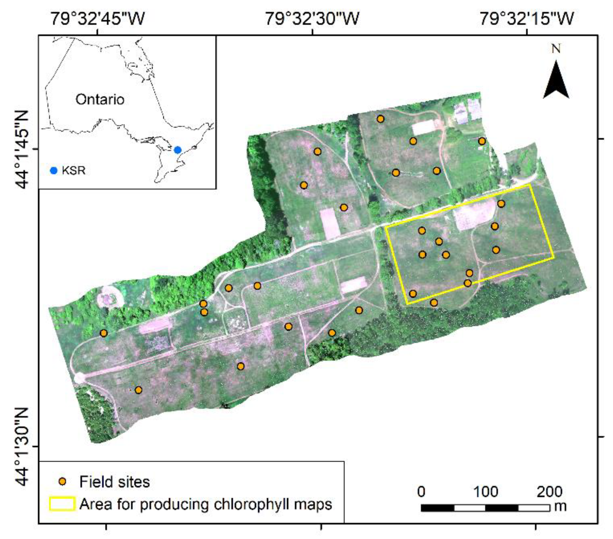
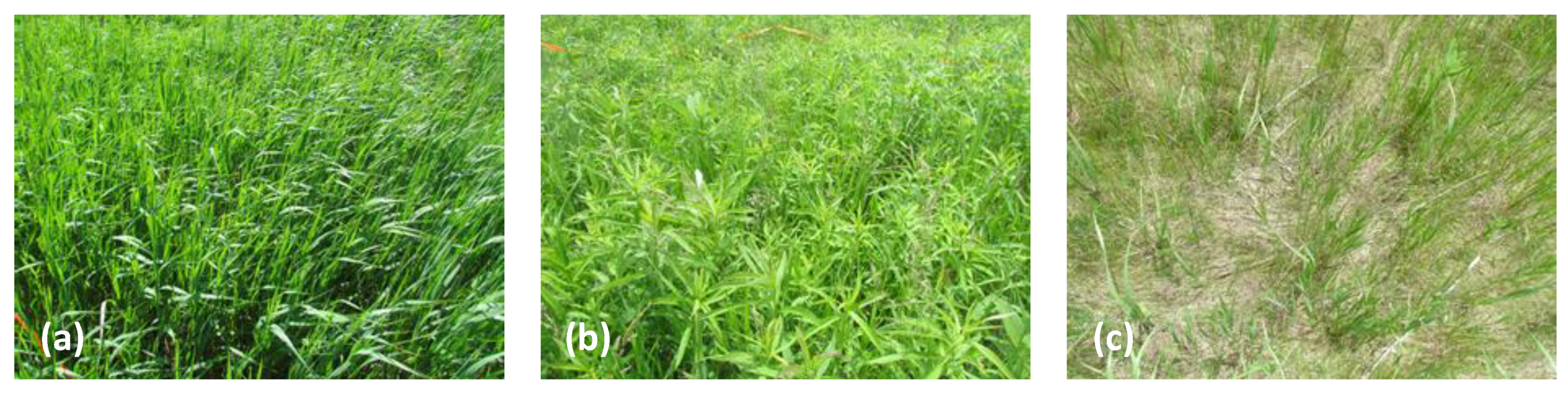
The study area of this research is Koffler Scientific Reserve (KSR) in King City, Ontario, Canada (Figure 1). This region has monthly mean temperatures ranging from −10 °C to 30 °C and monthly mean precipitations from 20 mm to 100 mm [25]. Dominant species in the study area include Awnless Brome (Bromus inermis), Goldenrod (Solidago canadensis L.), and Fescue (Festuca rubra L.). There are three major types of canopies in terms of species composition during the fast-growing season (e.g., May to July), including Awnless Brome, Goldenrod, and sparse canopies with mixed Fescue and Awnless Brome (hereafter named as Fescue canopies). Photos of these three types of canopies are shown in Figure 2.
2.2. Field Data Collection
Field surveys were conducted in June 2016. A total of 29 field sites covering different species compositions were deployed in the study area using a stratified sampling approach (e.g., more samples were collected for more dominant species). Each site was a 2 m × 2 m square, divided into four quarter sections as four study plots with each plot sized 1 m × 1 m. As a result, we built a total of 116 study plots. Field and remote sensing data collected from these study plots were used to establish analytical models and estimate canopy chlorophyll content.
A range of field data, including GPS, leaf area index, species composition, and photos, were collected for each plot. Specifically, GPS information was obtained using a Trimble GeoExplorer with centimeter-level accuracy (Trimble Navigation Limited, Sunnyvale, CA, USA). Leaf area index of each plot was measured with an AccuPAR LP-80 ceptometer (Decagon Devices, Inc., Pullman, Washington, DC, USA). Species composition information of each plot was visually interpreted in the field. In total, 68 plots were identified as Awnless Brome, 32 as Fescue, and 16 as Goldenrod. In addition, leaf samples were also collected to measure chlorophyll concentration using N, N-dimethylformamide (DMF) in a wet lab and converted to chlorophyll content [26]. Canopy-level chlorophyll was then calculated by multiplying the leaf area index with leaf chlorophyll content [21,27]. As different species have various canopy structures and leaf characteristics, their canopy chlorophyll contents have different data distribution patterns (e.g., chlorophyll content of one species is substantially higher than that of others). Canopy chlorophyll contents of the three dominant species (Awnless Brome, Fescue, and Goldenrod) were thus plotted against a spectral index in order to investigate their data distribution patterns (more details in the following section).
2.3. Collection and Processing of Hyperspectral Imagery
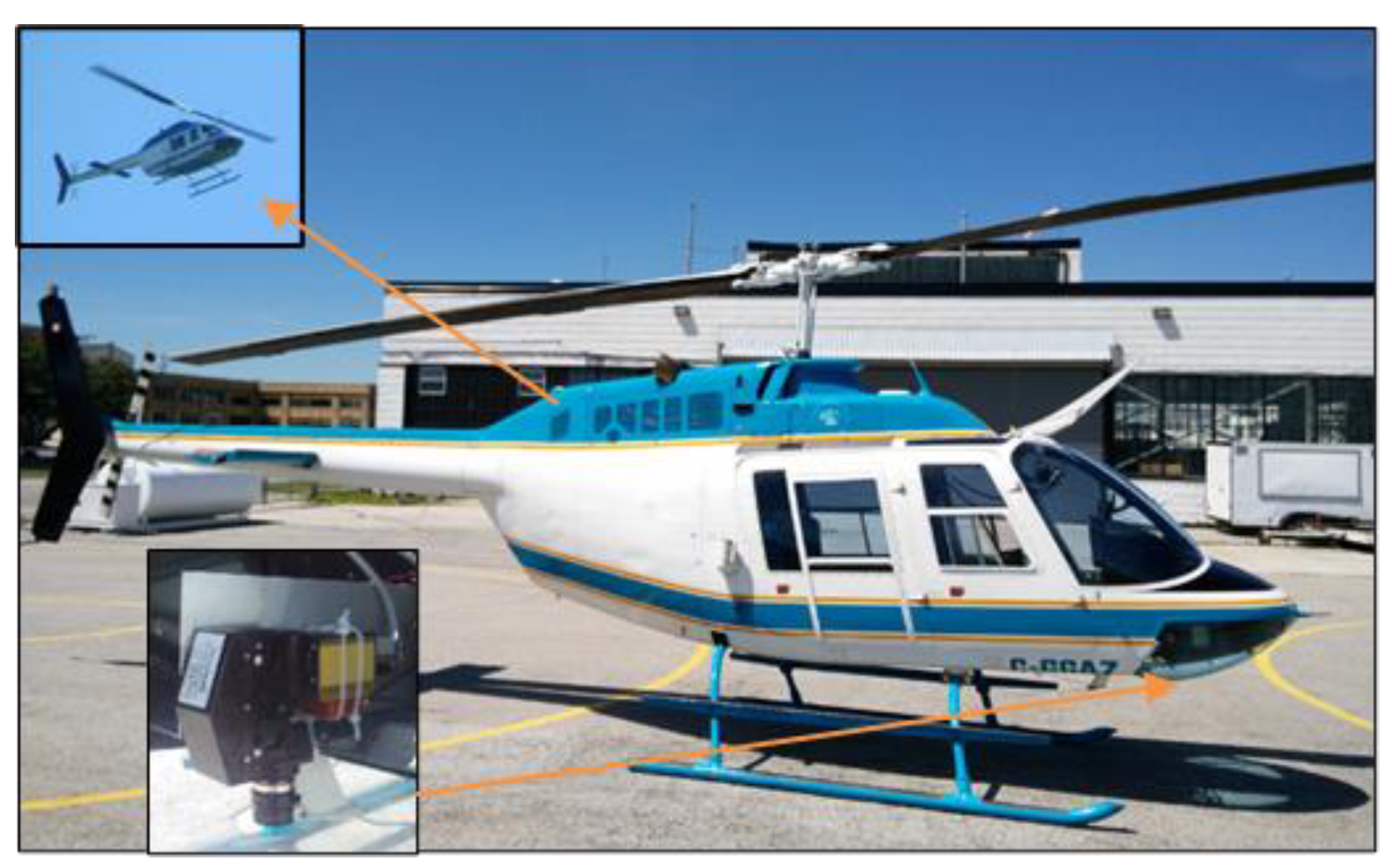
The sensor used in this study was a Micro-HyperSpec developed by Headwall Photonics Inc. (Boston, MA, USA). It has 325 bands in the visible to near infrared region. The sensor was installed on a helicopter to achieve an extended flight time and high stability (Figure 3). The flight was conducted around noon on 14 June 2016, with a flight height of about 250 m. The spatial resolution of images obtained at this height was 30 cm. The raw image data were radiometrically corrected using correction coefficients provided by Headwall Photonics Inc., followed by geometric correction using data from GPS and inertial measurement unit (IMU) that were mounted on the sensor. Lastly, an atmospheric correction was performed using an empirical line method in ENVI [28]. More details of data collection and preprocessing can be found in [29,30].
Hyperspectral features were then extracted from the image to estimate canopy chlorophyll content. It has been confirmed in our previous studies that band reflectance, principal components (PCs), spectral indices, and texture metrics can all contribute to the retrieval of chlorophyll content [16,31]. Therefore, these different types of variables were calculated in this study. Specifically, 31 reflectance data were extracted with a 20 nm interval (e.g., from 400, 420, 440, to 980, and 1000 nm) (Table 1), aiming to remove correlated bands and reduce the computing load. The top 5 PCs that included the majority of information from the hyperspectral images were obtained in ENVI and named as PC1 to PC5 [32]. Twenty-one spectral indices confirmed to be sensitive to vegetation properties were also calculated (Table 1) [33,34,35]. Lastly, texture metrics of selected spectral bands were also calculated in ENVI. Specifically, it was found that reflectance values at 450, 550, 670, 680, 704, 750, and 800 nm have been more commonly used in spectral indices for estimating chlorophyll content, indicating their high sensitivity to this pigment [16]. Therefore, eight texture metrics (e.g., variance, contrast, and entropy) of each of these seven spectral bands were calculated, resulting in 56 texture metrics (Table 1). A total of 113 features (including 31 reflectance, 5 PCs, 21 indices, and 56 texture metrics) were thus obtained and used as predictor variables in analytical models.
2.4. Establishment of Different Models for Estimating Chlorophyll
The canopy chlorophyll content and hyperspectral variables (Table 1), as the response and predictor variables, were used for building LR and RFR models. As mentioned in the Introduction, species composition might have impacts on the accuracy of estimating canopy chlorophyll content if using different modelling approaches (i.e., a universal model versus species-specific models). Therefore, four models were examined, including (1) a universal LR model trained with data of all three dominant species (i.e., Awnless Brome, Goldenrod, and Fescue); (2) species-specific LR models trained with data of each species, respectively (i.e., LR of Awnless Brome, LR of Goldenrod, and LR of Fescue); (3) a universal RFR model trained with data of all three dominant species; and (4) species-specific RFR models trained with data of each species, respectively.
The LR and RFR models were built using Python [36]. For LR models, each of 113 predictor variables (Table 1) was used for building an LR model. In RFR models, all 113 predictor variables were used, aiming to better explore and utilize spectral and textural information in these variables. The importance of each variable was also calculated in RFR for evaluating its potential contribution to the model [37]. The number of trees to grow in RFR models was tested using 100, 200, 500, 1000, and 2000, aiming to identify a parameter that could generate better model performance [38,39,40,41]. The minimum number of samples required to be at a leaf node was set to 1, and all variables were tested at each splitting node [37,39]. A leave-one-out cross-validation method was utilized for validating the four models. Lastly, the universal LR model, species-specific LR models, universal RFR model, and species-specific RFR models were compared. The model with the highest coefficient of determination (R2) and lowest root mean square error (RMSE) was identified as the best-performed model. The impacts of the species composition on the estimation accuracy of chlorophyll content were then discussed. Lastly, the best-performed model was used for producing chlorophyll content maps.
2.5. Object-Based Species Classification and Chlorophyll Mapping
One goal of this research is to produce a species-specific chlorophyll content map for each of the three dominant species (i.e., Awnless Brome, Goldenrod, and Fescue, shown in Figure 2). Image classification was thus performed to identify these species. An object-based image analysis method was conducted to segment the hyperspectral image to objects that represent different clusters of species. The segmentation was performed using ENVI Feature Extraction (L3Harris Geospatial, Broomfield, CO, USA). The 113 band layers were used for segmentation. A scale parameter of 0.1 and a merge parameter of 0.1 were used for producing objects that could represent different species patches. Information on the 113 bands (i.e., 31 reflectance, 5 PCs, 21 indices, and 56 texture metrics) was passed to the objects, which was used for classification. A random forest classification model was built using Python and then used for species classification [36]. The number of trees in the forest was set to 500, the minimum number of samples required to be at a leaf node was set to 1, and all features were considered for splitting each node [36,42,43]. Samples for training and validating the classification model included the study plots mentioned in the field survey section and additional plots collected only for the species classification. A total of 343 samples of Awnless Brome, 145 samples of Fescue, and 98 samples of Goldenrod were identified. Half of these samples were used for training the classification model and the other half for validation (i.e., calculation of confusion matrix). After the classification model was validated, objects of different species and the corresponding band information were used for estimating chlorophyll content using the best-performed models identified in the previous section. Lastly, species-specific chlorophyll content maps were produced, and variations of chlorophyll were thus investigated. Considering the computation demand and purpose of demonstration, the part of the study area that featured a mixture of the three species was used to produce the maps (Figure 1).
3. Results and Discussion
3.1. Data Distribution Patterns of Different Species
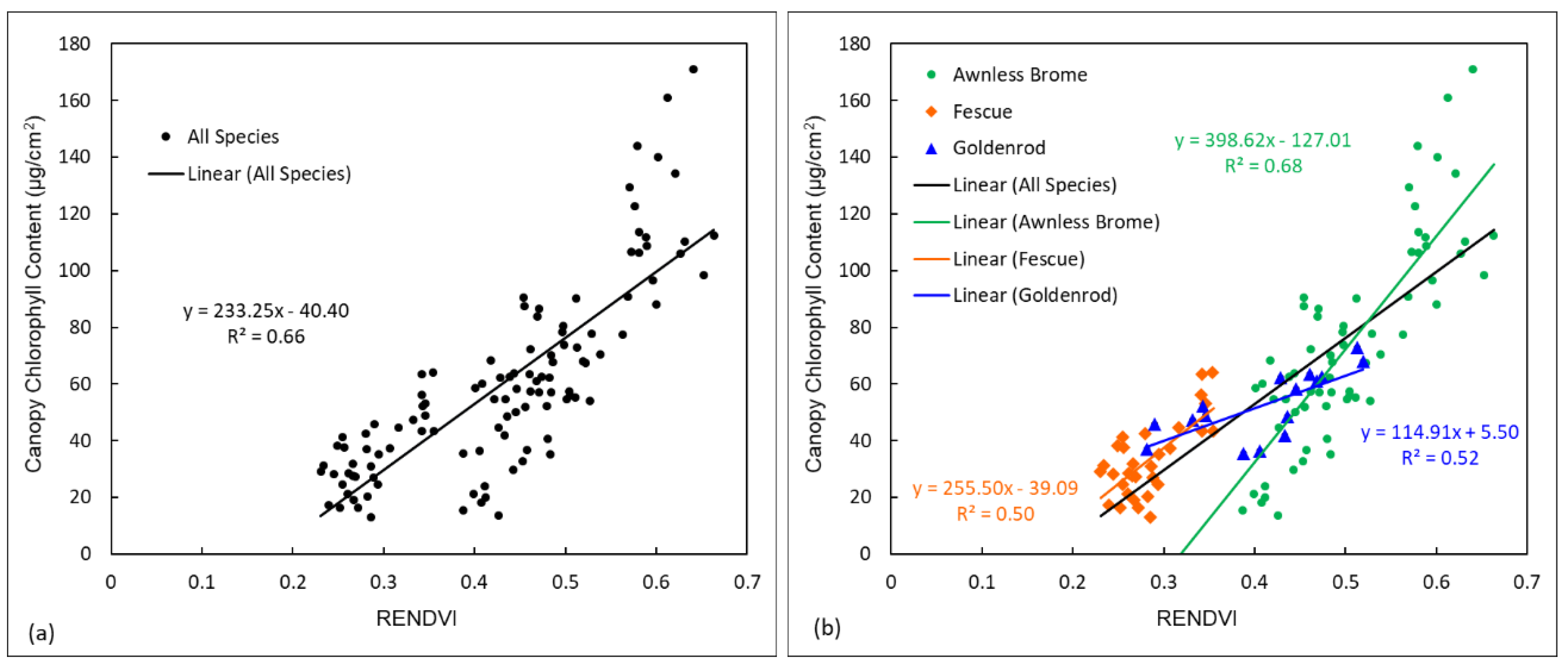
Canopy chlorophyll contents of three dominant species (Awnless Brome, Fescue, and Goldenrod) were plotted against RENDVI, a top-performed spectral index for estimating chlorophyll, aiming to observe distribution patterns of the chlorophyll values (Figure 4). Data of all three species were plotted together in Figure 4a, and three species were plotted separately in Figure 4b. It can be found that data of the three species had very different distribution patterns (Figure 4b). For instance, the chlorophyll contents of Awnless Brome were generally higher (e.g., >50 µg/cm2), those of Fescue were generally lower (e.g., <50 µg/cm2), and those of Goldenrod were in between (Figure 4b). The slope of the regression line for Fescue (e.g., 255.50) was close to that of all three species together (e.g., 233.25), while that of Awnless Brome was much larger (e.g., 398.62), but that of Goldenrod was much smaller (e.g., 114.91). Therefore, if building a universal linear regression model for estimating chlorophyll contents of all three species together, the different data distribution patterns would be ignored. The estimation accuracy may not be high for each species, although it could be high for all three species together. This hypothesis was examined and discussed in the next section.
We also found the saturation issue of using spectral indices for estimating properties of green and dense vegetation (Figure 4a). Specifically, when the chlorophyll contents were higher than 120 µg/cm2, the RENDVI values remained around 0.6. The saturation issue has been widely discussed in previous studies [38,39,44], indicating the potential limitation of using LR and spectral indices for estimating vegetation properties, which is another reason why RFR was also applied in this research for estimating chlorophyll content.
3.2. Comparison of Different Modelling Approaches for Estimating Chlorophyll
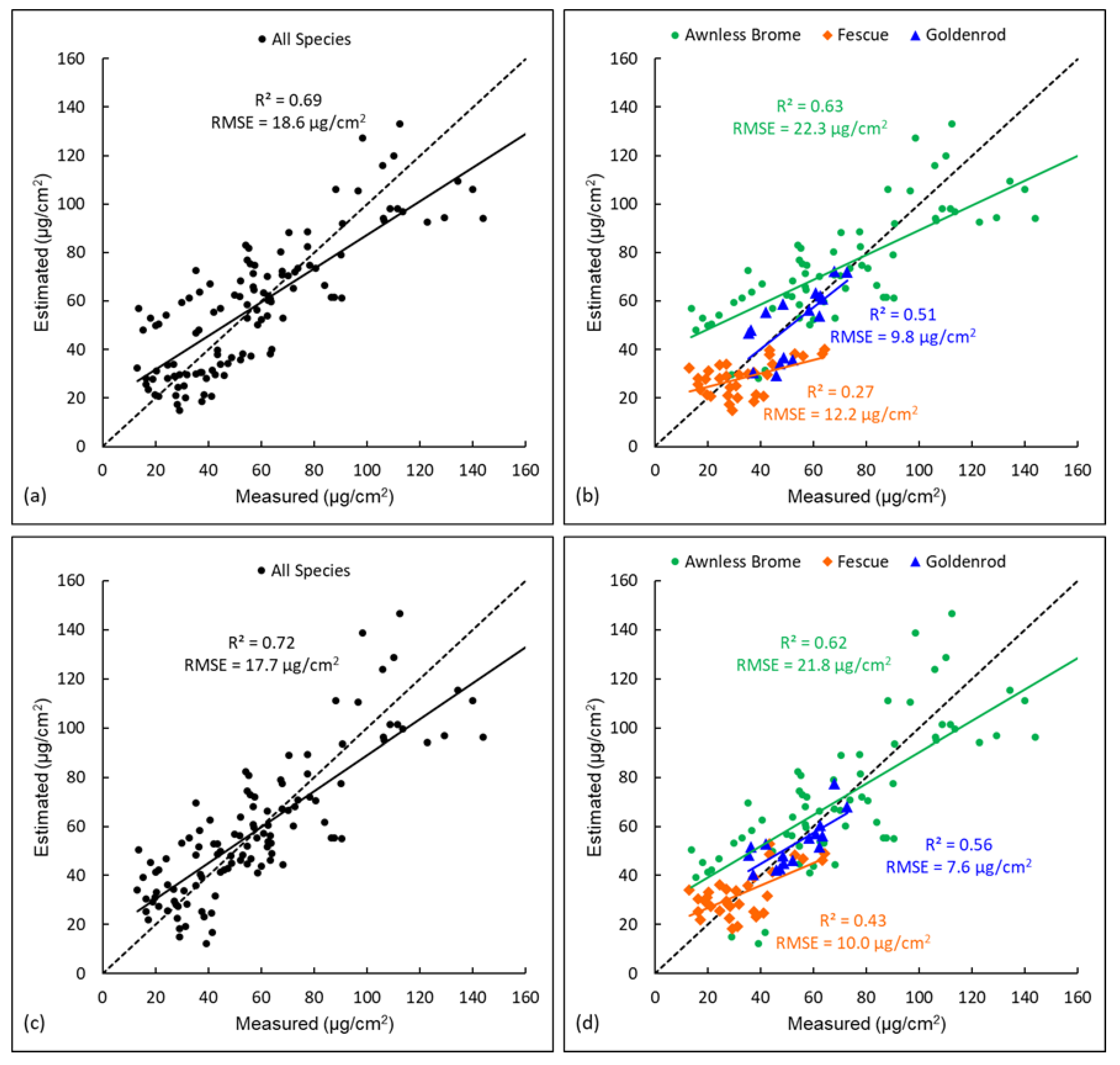
Four models, including a universal LR model (i.e., trained with data of all three dominant species), species-specific LR models (i.e., trained with data of each species), a universal RFR model, and species-specific RFR models, were established and validated (with R2 and RMSE as metrics), aiming to compare their accuracies for chlorophyll estimation. Validation results of the two LR models are shown in Figure 5. For the universal LR model established with all species (Figure 5a), it was validated with all species data together and achieved a satisfactory accuracy with R2 = 0.69 and RMSE = 18.6 µg/cm2. In addition to this validation with all species to understand the overall model performance, it was also critical to understand the model accuracy for each specific species. Therefore, the model was then validated with data of each species, and it was found this universal LR had largely varied accuracies for the three species (Figure 5b). Specifically, the accuracy for Awnless Brome (R2 = 0.63 and RMSE = 22.3 µg/cm2) was close to that of the overall accuracy. This is mainly because Awnless Brome is the dominant species and had 68 of the total 116 samples, in addition to the fact that it has a wide range of chlorophyll content (e.g., 20~140 µg/cm2), which can highly influence the regression. However, the model accuracy was lower for Goldenrod (R2 = 0.51 and RMSE = 9.8 µg/cm2) and much lower for Fescue (R2 = 0.27 and RMSE = 12.2 µg/cm2). This is because, compared to Awnless Brome, there were fewer training samples of these two species (i.e., 32 for Fescue and 16 for Goldenrod) in the regression, and their ranges of chlorophyll content were also smaller (i.e., 15–60 µg/cm2 for Fescue and 35–70 µg/cm2 for Goldenrod). Data of these two species thus had fewer impacts on the regression, causing their lower estimation accuracies. Therefore, when evaluated by pulling data from all species, a model with good performance does not necessarily mean the model performance will be similarly good for each specific species, especially for species with fewer training samples used in the model or with small value ranges. This also reveals the influence of sample sizes of different species on the estimation accuracy. In this study, a stratified sampling approach was used, and more samples were thus collected for Awnless Brome as it is more dominant. If using another sampling approach, such as collecting the same number of samples for all species, the estimation accuracies of different species may change. Therefore, the sampling approach should also be considered in the estimation of properties of different species.
Species-specific LR models were validated, and the results are shown in Figure 5d. Compared to the accuracies of the universal LR model (Figure 5b), it can be found that the accuracies of Awnless Brome were close (e.g., R2 = 0.62 and RMSE = 21.8 µg/cm2 for the species-specific model versus R2 = 0.63 and RMSE = 22.3 µg/cm2 for the universal model). This is because, as discussed previously, Awnless Brome with most samples dominated the data distribution. However, the accuracies for Goldenrod were improved from R2 = 0.51 and RMSE = 9.8 µg/cm2 produced by the universal model to R2 = 0.56 and RMSE = 7.6 µg/cm2 from the species-specific model. Similarly, the accuracies for Fescue were largely improved from R2 = 0.27 and RMSE = 12.2 µg/cm2 to R2 = 0.43 and RMSE = 10.0 µg/cm2. These improvements were due to the fact that the species-specific models are capable of capturing the data patterns of each species. In addition, the results of three species-specific models were also validated by combining data of all three species, and the results are shown in Figure 5c. The utilization of species-specific models also slightly improved the estimation accuracy for the three species overall, i.e., from R2 = 0.69 and RMSE = 18.6 µg/cm2 to R2 = 0.72 and RMSE = 17.7 µg/cm2. In summary, species-specific LR models can generate higher estimation accuracy than a universal LR. This is especially true for less-dominant species with fewer training samples and smaller ranges of vegetation properties (e.g., chlorophyll content).
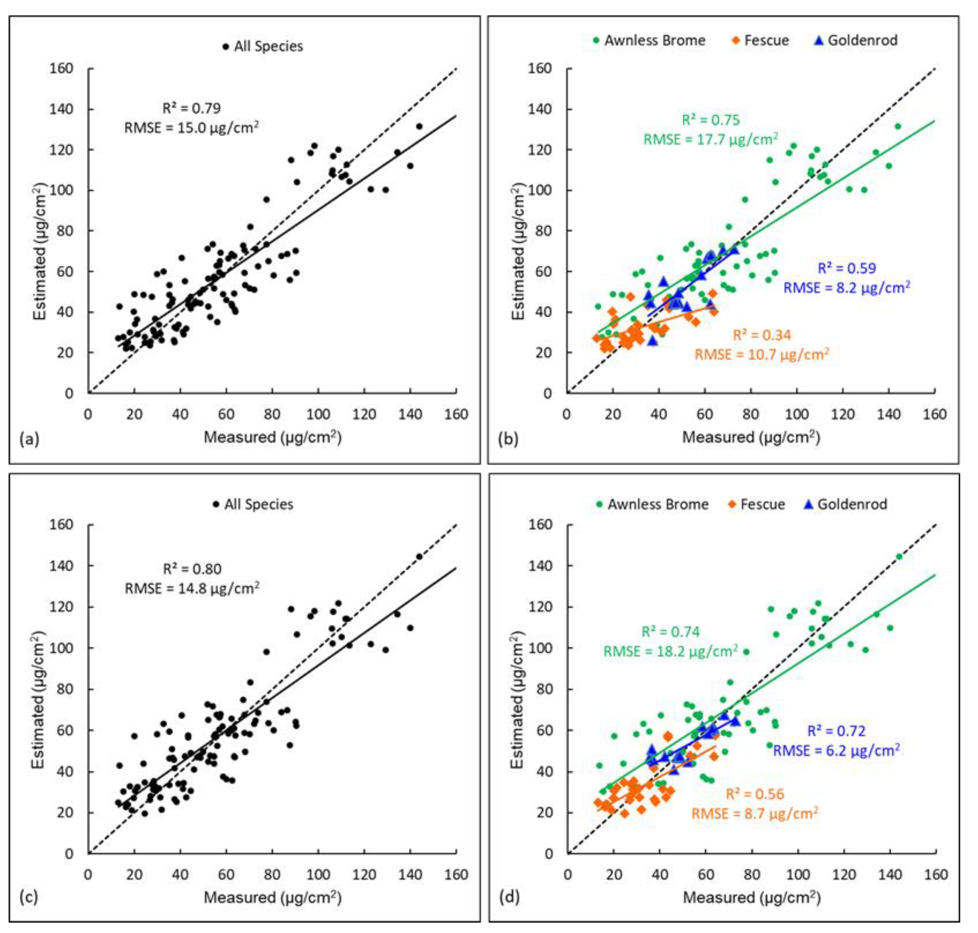
A universal RFR model was also established using data of all three species together and validated (Figure 6a). This model achieved an accuracy with R2 = 0.79 and RMSE = 15.0 µg/cm2, which was higher than that of the universal LR model with R2 = 0.69 and RMSE = 18.6 µg/cm2 (Figure 5a). This is because the RFR model is capable of using multiple predictor variables in the model and selecting more important ones for splitting the trees, and thus it has a much higher predicting power than the LR. This universal RFR model was also validated using data of each specific species and the results are shown in Figure 6b. Compared to the overall accuracy of all three species (R2 = 0.79 and RMSE = 15.0 µg/cm2, Figure 6a), the accuracy of Awnless Brome was close (R2 = 0.75 and RMSE = 17.7 µg/cm2), while the accuracy of Goldenrod (R2 = 0.59 and RMSE = 8.2 µg/cm2) was lower, followed by that of Fescue (R2 = 0.34 and RMSE = 10.7 µg/cm2) (Figure 6b). A similar finding was also noticed for the universal LR model (Figure 5a,b), and the reasons would be similar, i.e., the Awnless Brome has more samples and a wider range of chlorophyll than those of Goldenrod and Fescue. It is also important to note that the universal RFR model achieved higher accuracies for each specific species (Figure 6b) than the universal LR model (Figure 5b); the accuracy of Awnless Brome was improved from R2 = 0.63 and RMSE = 22.3 µg/cm2 in the universal LR to R2 = 0.75 and RMSE = 17.7 µg/cm2 in the universal RFR, the accuracy of Goldenrod was improved from R2 = 0.51 and RMSE = 9.8 µg/cm2 to R2 = 0.59 and RMSE = 8.2 µg/cm2, and the accuracy of Fescue was improved from R2 = 0.27 and RMSE = 12.2 µg/cm2 to R2 = 0.34 and RMSE = 10.7 µg/cm2. These suggest clearly better performance of the RFR over LR. Therefore, the RFR model is recommended for similar studies to estimate vegetation features using remote sensing.
Species-specific RFR models were also established and validated, and the results are shown in Figure 6d. Compared to the universal RFR model (Figure 6b), the accuracies of Awnless Brome were close in the two models (R2 ~ 0.75 and RMSE ~ 18.0 µg/cm2). However, the accuracy of Goldenrod was improved from R2 = 0.59 and RMSE = 8.2 µg/cm2 in the universal RFR to R2 = 0.72 and RMSE = 6.2 µg/cm2 in the species-specific RFR, and the accuracy of Fescue was improved from R2 = 0.34 and RMSE = 10.7 µg/cm2 to R2 = 0.56 and RMSE = 8.7 µg/cm2 (Figure 6b,d). Similar findings were also observed for the universal LR versus species-specific LR models (Figure 5b,d). This further confirms the impacts of using universal models on the accuracies of estimating vegetation properties, especially for the species that have fewer training samples included in the model. Comparing the results of species-specific LR (Figure 5d) and that of species-specific RFR (Figure 6d), accuracies of all three species were improved. Specifically, the accuracy of Awnless Brome was improved from R2 = 0.62 and RMSE = 21.8 µg/cm2 in the species-specific LR to R2 = 0.74 and RMSE = 18.2 µg/cm2 in species-specific RFR, the accuracy of Goldenrod was improved from R2 = 0.56 and RMSE = 7.6 µg/cm2 to R2 = 0.72 and RMSE = 6.2 µg/cm2, and the accuracy of Fescue was improved from R2 = 0.43 and RMSE = 10.0 µg/cm2 to R2 = 0.56 and RMSE = 8.7 µg/cm2. This also indicates the better performance of RFR than LR, as discussed previously, owing to the fact that RFR is capable of evaluating the importance of predictor variables and selecting more important ones for improving estimation accuracy.
To understand which variables are more important in the universal and species-specific RFR models for predicting chlorophyll contents, the top 10 important variables in each model were identified. As the variables that are important in the species-specific models may also be, or not, important in the universal RFR, they were listed in Table 2 for comparisons. Nine of the top 10 important variables in the Awnless Brome model were also among the top 10 for the universal model, including VREI1, b680-Mean, RENDVI, and MRENDVI, etc. However, only 3 of the top 10 important variables in the Fescue model were among the top 10 for the universal model, which were RENDVI, VREI1, and RGRI. Similarly, only 2 of the top 10 important variables in the Goldenrod model were among the top 10 for the universal model, and these are RGRI and NDVI. Most of the variables that were important in the Fescue or Goldenrod models are not among the top 10 important ones for the universal model, such as SIPI, PC3, and b680-Correlation for the Fescue model, and Re740, PC1, and Re900 for the Goldenrod model. This also explains the lower estimation accuracies for Fescue and Goldenrod in the universal model, as the important variables for these two species were not rated as important for the universal model. In contrast, the most important variables for the Awnless Brome model were also important in the universal model, which indicates that data of Awnless Brome drove the regression model and contributed to the high estimation accuracy for this species. In addition, different types of variables (e.g., reflectance, PCs, indices, and texture metrics) were among the top 10 important ones in the universal or species-specific RFR models (Table 2). This indicates that they have different information that can all contribute to the model predictions. Therefore, calculating multi-type variables is recommended for estimating vegetation properties using remote sensing.
3.3. Object-Based Species Classification
The hyperspectral imagery was segmented into objects that represented different species patches, and the objects were then classified into different species. Classification accuracies were evaluated, and the results are shown in Table 3. The classification model had an overall accuracy of 94% and a kappa coefficient of 88%, indicating good performance of the model. Producer’s and User’s accuracy values of the three species were mostly higher than 90%, but the Producer’s accuracy of Goldenrod was 77%. There were eight and five Goldenrod samples that were misclassified as Awnless Brome and Fescue, respectively (Table 3). Sometimes Goldenrod and Awnless Brome/Fescue are mixed in one object, while the 30 cm resolution is not sufficient to identify each and thus misclassifies. Using images with higher spatial resolution may improve classification accuracy.
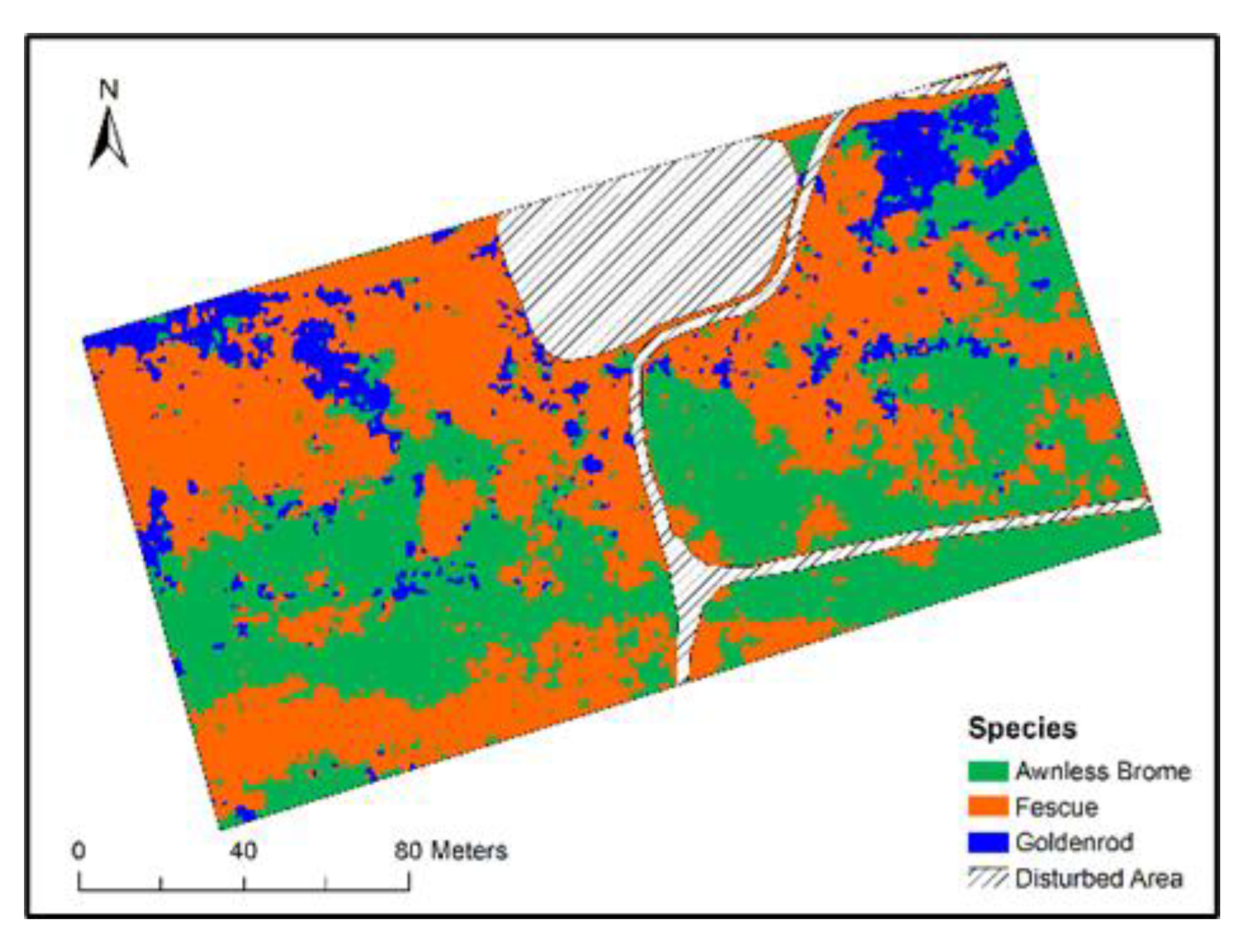
Species classification map is shown in Figure 7. Clear spatial variations of species can be observed from the map. For example, Goldenrod plants are mainly seen in the north-western and north-eastern corners of the mapped area, Awnless Brome plants are mostly in the central part from west to east, and Fescue plants are in the other areas.
3.4. Mapping Species-Specific Chlorophyll Contents
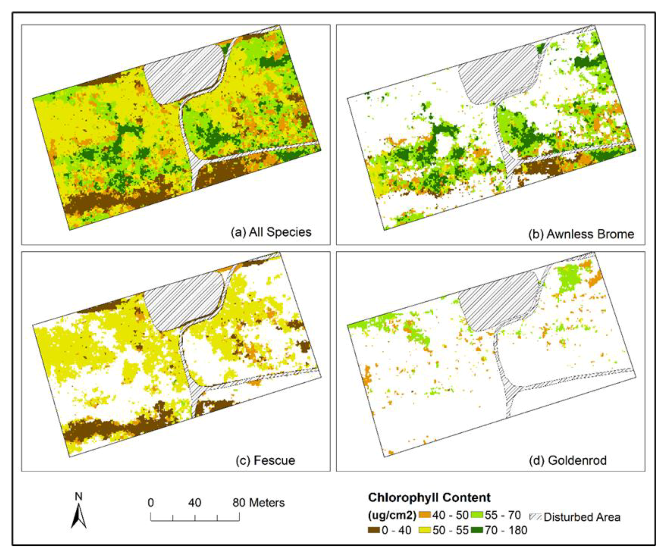
Objects of classified species and corresponding spectral and textural information were used for producing chlorophyll content maps using the optimal models (i.e., species-specific RFR) identified in Section 3.2. A combined chlorophyll map of all species and species-specific maps are shown in Figure 8. Spatial variations of chlorophyll contents of different species can be observed.
As discussed in previous sections (e.g., Figure 4), the Awnless Brome generally had higher chlorophyll contents, Fescue’s chlorophyll was relatively lower, and Goldenrod was in between, which can also be observed in the chlorophyll content maps (Figure 8b–d). For example, most areas with Awnless Brome had chlorophyll contents higher than 50 µg/cm2, and areas with chlorophyll lower than this value were mostly in the south-eastern section of the mapped area (Figure 8b). Areas with Fescue generally had chlorophyll contents lower than 55 µg/cm2 (Figure 8c). One area with chlorophyll less than 40 µg/cm2 was found in the south-western section (i.e., the large brown-color area in Figure 8c). This is a crest area with limited soil moisture, which is more suitable for the growth of Fescue. In terms of Goldenrod, its distribution range was much smaller than that of the other two species, and it generally had chlorophyll contents in the range of 40–70 µg/cm2 (Figure 8d). Overall, the species-specific chlorophyll maps contribute greatly to the interpretation of species distribution and corresponding chlorophyll contents, which is critical for understanding the physiological status of different species and the overall ecosystem conditions. Generating species-specific maps of various vegetation properties (e.g., chlorophyll content, leaf area index, biomass) is thus recommended, especially for heterogeneous ecosystems (e.g., grasslands and wetlands).
4. Summary
Ecosystems such as grasslands and wetlands are heterogeneous with mixed species. Mapping species-specific vegetation properties (e.g., chlorophyll content) is critical for understanding their distributions, growth conditions, and ecosystem health. This is especially true for mapping and investigating invasive species that is a considerable issue in many ecosystems. Universal models that are generally built with data of all species have been commonly used in previous studies for mapping vegetation properties using remote sensing. Data distribution patterns of specific species are ignored in such universal models, which may affect the estimation accuracies of each specific species. In this study, a universal LR and species-specific LR models as well as a universal RFR and species-specific RFR models were built using data of three dominant species in a heterogeneous grassland. Their performances were examined and compared to evaluate the impacts of species composition on the retrieval accuracy of chlorophyll content.
The results showed that the species-specific models generated higher accuracies than the universal models for species that were less dominant (i.e., Fescue and Goldenrod that had fewer training samples in the dataset and narrow ranges of chlorophyll contents, Figure 5 and Figure 6). In contrast, the species-specific models and the universal models had similar accuracies for species that were more dominant (i.e., Awnless Brome with more training samples in the dataset and a wide range of chlorophyll content). This indicates that data of the more dominant species will drive the universal models (regardless of using LR or RFR), which will reduce the accuracy of less dominant species. Most of top 10 important variables in the RFR model of Awnless Brome were among the top 10 important ones in the universal RFR, but this was not the case for the RFR models of Fescue and Goldenrod (Table 2). Important variables in these two species-specific models mostly were not among the important ones in the universal model, which thus caused the low accuracies for chlorophyll estimations of these two species.
Overall, utilization of species-specific models is recommended for mapping vegetation properties in heterogeneous ecosystems, especially if the research focus is on less dominant species (i.e., species with fewer training samples collected or if they have narrow ranges of vegetation properties). It will be critical to plot the property data of different species (e.g., against a popular spectral index as shown in Figure 4) and check the data distribution patterns of these species. Then more informed decisions of model selections can be made. In addition, RFR models performed consistently better than the LR models owing to their capabilities of utilizing multiple predictor variables that can improve the predicting power of the model. There are other advanced analytical models that have been developed for estimating vegetation properties, including artificial intelligence algorithms, which can be explored to further improve estimation accuracy [45,46]. Further, multiple types of variables (e.g., reflectance, indices, principal components, and texture metrics) contain different information that can all contribute to the estimation of vegetation properties (Table 2). Therefore, the calculation of such different types of variables is also important for improving the model performance.
Author Contributions
Conceptualization, B.L.; formal analysis, B.L.; funding acquisition, B.L. and Y.H.; investigation, B.L. and Y.H.; methodology, B.L. and Y.H.; project administration, B.L. and Y.H.; resources, B.L. and Y.H.; software, B.L. and Y.H.; supervision, B.L. and Y.H.; validation, B.L.; visualization, B.L.; writing—original draft, B.L.; writing—review and editing, B.L. and Y.H. All authors have read and agreed to the published version of the manuscript.
Funding
This research was funded by the Natural Sciences and Engineering Research Council of Canada, Discovery Grant [RGPIN-386183] to Yuhong He, and Simon Fraser University New Faculty Start-Up Grant to Bing Lu.
Acknowledgments
We thank a group of research assistants from the Remote Sensing and Spatial Ecosystem Modeling laboratory at the University of Toronto Mississauga who helped with field and lab work and the managers of the Koffler Scientific Reserve.
Conflicts of Interest
The authors declare no conflict of interest.
References
- Blackburn, G.A. Hyperspectral remote sensing of plant pigments. J. Exp. Bot. 2007, 58, 855–867. [Google Scholar] [CrossRef] [PubMed] [Green Version]
- Dong, T.; Shang, J.; Chen, J.M.; Liu, J.; Qian, B.; Ma, B.; Morrison, M.J.; Zhang, C.; Liu, Y.; Shi, Y.; et al. Assessment of Portable Chlorophyll Meters for Measuring Crop Leaf Chlorophyll Concentration. Remote Sens. 2019, 11, 2706. [Google Scholar] [CrossRef] [Green Version]
- Shang, J.; Liu, J.; Ma, B.; Zhao, T.; Jiao, X.; Geng, X.; Huffman, T.; Kovacs, J.M.; Walters, D. Mapping spatial variability of crop growth conditions using RapidEye data in Northern Ontario, Canada. Remote Sens. Environ. 2015, 168, 113–125. [Google Scholar] [CrossRef]
- Moharana, S.; Dutta, S. Spatial variability of chlorophyll and nitrogen content of rice from hyperspectral imagery. ISPRS J. Photogramm. 2016, 122, 17–29. [Google Scholar] [CrossRef]
- Wu, C.; Han, X.; Niu, Z.; Dong, J. An evaluation of EO-1 hyperspectral Hyperion data for chlorophyll content and leaf area index estimation. Int. J. Remote Sens. 2010, 31, 1079–1086. [Google Scholar] [CrossRef]
- Haboudane, D.; Tremblay, N.; Miller, J.R.; Vigneault, P. Remote estimation of crop chlorophyll content using spectral indices derived from hyperspectral data. IEEE T. Geosci. Remote 2008, 46, 423–437. [Google Scholar] [CrossRef]
- Lemaire, G.; Francois, C.; Soudani, K.; Berveiller, D.; Pontailler, J.; Breda, N.; Genet, H.; Davi, H.; Dufrene, E. Calibration and validation of hyperspectral indices for the estimation of broadleaved forest leaf chlorophyll content, leaf mass per area, leaf area index and leaf canopy biomass. Remote Sens. Environ. 2008, 112, 3846–3864. [Google Scholar] [CrossRef]
- Croft, H.; Chen, J.M.; Zhang, Y.; Simic, A.; Noland, T.L.; Nesbitt, N.; Arabian, J. Evaluating leaf chlorophyll content prediction from multispectral remote sensing data within a physically-based modelling framework. ISPRS J. Photogramm. 2015, 102, 85–95. [Google Scholar] [CrossRef]
- Croft, H.; Arabian, J.; Chen, J.M.; Shang, J.; Liu, J. Mapping within-field leaf chlorophyll content in agricultural crops for nitrogen management using Landsat-8 imagery. Precis. Agric. 2019, 21, 856–880. [Google Scholar] [CrossRef] [Green Version]
- Zhou, X.; Zhang, J.; Chen, D.; Huang, Y.; Kong, W.; Yuan, L.; Ye, H.; Huang, W. Assessment of Leaf Chlorophyll Content Models for Winter Wheat Using Landsat-8 Multispectral Remote Sensing Data. Remote Sens. 2020, 12, 2574. [Google Scholar] [CrossRef]
- Yu, F.; Xu, T.; Du, W.; Ma, H.; Zhang, G.; Chen, C. Radiative transfer models (RTMs) for field phenotyping inversion of rice based on UAV hyperspectral remote sensing. Int. J. Agric. Biol. Eng. 2017, 10, 150–157. [Google Scholar]
- Croft, H.; Chen, J.M.; Zhang, Y.; Simic, A. Modelling leaf chlorophyll content in broadleaf and needle leaf canopies from ground, CASI, Landsat TM 5 and MERIS reflectance data. Remote Sens. Environ. 2013, 133, 128–140. [Google Scholar] [CrossRef]
- Croft, H.; Chen, J.M.; Zhang, Y. The applicability of empirical vegetation indices for determining leaf chlorophyll content over different leaf and canopy structures. Ecol. Complex. 2014, 17, 119–130. [Google Scholar] [CrossRef]
- Simic, A.; Chen, J.M.; Noland, T.L. Retrieval of forest chlorophyll content using canopy structure parameters derived from multi-angle data: The measurement concept of combining nadir hyperspectral and off-nadir multispectral data. Int. J. Remote Sens. 2011, 32, 5621–5644. [Google Scholar] [CrossRef]
- Wong, K.K.; He, Y. Estimating grassland chlorophyll content using remote sensing data at leaf, canopy, and landscape scales. Can. J. Remote Sens. 2013, 39, 155–166. [Google Scholar] [CrossRef]
- Lu, B.; He, Y. Evaluating Empirical Regression, Machine Learning, and Radiative Transfer Modelling for Estimating Vegetation Chlorophyll Content Using Bi-Seasonal Hyperspectral Images. Remote Sens. 2019, 11, 1979. [Google Scholar] [CrossRef] [Green Version]
- Lu, B.; He, Y.; Liu, H.H.T. Mapping vegetation biophysical and biochemical properties using unmanned aerial vehicles-acquired imagery. Int. J. Remote Sens. 2018, 39, 5265–5287. [Google Scholar] [CrossRef]
- Guo, C.; Guo, X. Estimating leaf chlorophyll and nitrogen content of wetland emergent plants using hyperspectral data in the visible domain. Spectrosc. Lett. 2016, 49, 180–187. [Google Scholar] [CrossRef]
- Zhuo, W.; Shi, R.; Wu, N.; Zhang, C.; Tian, B. Spectral response and the retrieval of canopy chlorophyll content under interspecific competition in wetlands—case study of wetlands in the Yangtze River Estuary. Earth Sci. Inform. 2021, 14, 1467–1486. [Google Scholar] [CrossRef]
- Kanning, M.; Kuehling, I.; Trautz, D.; Jarmer, T. High-Resolution UAV-Based Hyperspectral Imagery for LAI and Chlorophyll Estimations from Wheat for Yield Prediction. Remote Sens. 2018, 10, 2000. [Google Scholar] [CrossRef] [Green Version]
- Darvishzadeh, R.; Atzberger, C.; Skidmore, A.; Schlerf, M. Retrieval of vegetation biochemicals using a radiative transfer model and hyperspectral data. In Proceedings of the ISPRS Technical Commission VII Symposium—100 Years ISPRS Advancing Remote Sensing Science, Vienna, Austria, 5–7 July 2010; Volume 38, pp. 171–175. [Google Scholar]
- Jacquemoud, S.; Verhoef, W.; Baret, F.; Bacour, C.; Zarco-Tejada, P.J.; Asner, G.P.; Francois, C.; Ustin, S.L. PROSPECT plus SAIL models: A review of use for vegetation characterization. Remote Sens. Environ. 2009, 113, S56–S66. [Google Scholar] [CrossRef]
- Belgiu, M.; Drăguţ, L. Random forest in remote sensing: A review of applications and future directions. ISPRS J. Photogramm. 2016, 114, 24–31. [Google Scholar] [CrossRef]
- Lu, B.; He, Y. Leaf Area Index Estimation in a Heterogeneous Grassland Using Optical, SAR, and DEM Data. Can. J. Remote Sens. 2019, 45, 618–633. [Google Scholar] [CrossRef]
- Historical Climate Data. Available online: http://climate.weather.gc.ca/ (accessed on 15 September 2021).
- Minocha, R.; Martinez, G.; Lyons, B.; Long, S. Development of a standardized methodology for quantifying total chlorophyll and carotenoids from foliage of hardwood and conifer tree species. Can. J. Forest Res. 2009, 39, 849–861. [Google Scholar] [CrossRef]
- Wong, K.K.L. Remote Sensing pf Tall Grasslands: Estimating Vegetation Biochemical Contents at Multiple Spatial Scales and Investigating Vegetation Temporal Response to Climate Conditions. Master’s Thesis, University of Toronto, Toronto, ON, Canada, 2013. [Google Scholar]
- Lucieer, A.; Malenovský, Z.; Veness, T.; Wallace, L. HyperUAS-imaging spectroscopy from a multirotor unmanned aircraft system. J. Field Robot. 2014, 31, 571–590. [Google Scholar] [CrossRef] [Green Version]
- Lu, B.; Proctor, C.; He, Y. Investigating different versions of PROSPECT and PROSAIL for estimating spectral and biophysical properties of photosynthetic and non-photosynthetic vegetation in mixed grasslands. GIScience Remote Sens. 2021, 58, 354–371. [Google Scholar] [CrossRef]
- Dao, P.D.; He, Y.; Lu, B. Maximizing the quantitative utility of airborne hyperspectral imagery for studying plant physiology: An optimal sensor exposure setting procedure and empirical line method for atmospheric correction. Int. J. Appl. Earth Obs. 2019, 77, 140–150. [Google Scholar] [CrossRef]
- Lu, B.; He, Y.; Dao, P.D. Comparing the Performance of Multispectral and Hyperspectral Images for Estimating Vegetation Properties. IEEE J. STARS 2019, 12, 1784–1797. [Google Scholar] [CrossRef]
- Were, K.; Bui, D.T.; Dick, O.B.; Singh, B.R. A comparative assessment of support vector regression, artificial neural networks, and random forests for predicting and mapping soil organic carbon stocks across an Afromontane landscape. Ecol. Indic. 2015, 52, 394–403. [Google Scholar] [CrossRef]
- Main, R.; Cho, M.A.; Mathieu, R.; O’Kennedy, M.M.; Ramoelo, A.; Koch, S. An investigation into robust spectral indices for leaf chlorophyll estimation. ISPRS J. Photogramm. 2011, 66, 751–761. [Google Scholar] [CrossRef]
- Tong, A.; He, Y. Estimating and mapping chlorophyll content for a heterogeneous grassland: Comparing prediction power of a suite of vegetation indices across scales between years. ISPRS J. Photogramm. 2017, 126, 146–167. [Google Scholar] [CrossRef]
- Spectral Indices. Available online: https://www.harrisgeospatial.com/docs/AlphabeticalListSpectralIndices.html (accessed on 10 December 2018).
- Pedregosa, F.; Varoquaux, G.; Gramfort, A.; Michel, V.; Thirion, B.; Grisel, O.; Blondel, M.; Prettenhofer, P.; Weiss, R.; Dubourg, V.; et al. Scikit-learn: Machine learning in Python. Mach. Learn. 2011, 12, 2825–2830. [Google Scholar]
- Yu, X.; Hyyppä, J.; Vastaranta, M.; Holopainen, M.; Viitala, R. Predicting individual tree attributes from airborne laser point clouds based on the random forests technique. ISPRS J. Photogramm. 2011, 66, 28–37. [Google Scholar] [CrossRef]
- Mutanga, O.; Adam, E.; Cho, M.A. High density biomass estimation for wetland vegetation using WorldView-2 imagery and random forest regression algorithm. Int. J. Appl. Earth Obs. 2012, 18, 399–406. [Google Scholar] [CrossRef]
- Adam, E.; Mutanga, O.; Abdel Rahman, E.M.; Ismail, R. Estimating standing biomass in papyrus (Cyperus papyrus L.) swamp: Exploratory of in situ hyperspectral indices and random forest regression. Int. J. Remote Sens. 2014, 35, 693–714. [Google Scholar] [CrossRef]
- Karlson, M.; Ostwald, M.; Reese, H.; Sanou, J.; Tankoano, B.; Mattsson, E. Mapping tree canopy cover and aboveground biomass in sudano-sahelian woodlands using Landsat 8 and random forest. Remote Sens. 2015, 7, 10017–10041. [Google Scholar] [CrossRef] [Green Version]
- Abdel-Rahman, E.M.; Ahmed, F.B.; Ismail, R. Random forest regression and spectral band selection for estimating sugarcane leaf nitrogen concentration using EO-1 Hyperion hyperspectral data. Int. J. Remote. Sens. 2013, 34, 712–728. [Google Scholar] [CrossRef]
- Lu, B.; He, Y. Species classification using Unmanned Aerial Vehicle (UAV)-acquired high spatial resolution imagery in a heterogeneous grassland. ISPRS J. Photogramm. 2017, 128, 73–85. [Google Scholar] [CrossRef]
- Lebourgeois, V.; Dupuy, S.; Vintrou, E.; Ameline, M.; Butler, S.; Begue, A. A Combined Random Forest and OBIA Classification Scheme for Mapping Smallholder Agriculture at Different Nomenclature Levels Using Multisource Data (Simulated Sentinel-2 Time Series, VHRS and DEM). Remote Sens. 2017, 9, 259. [Google Scholar] [CrossRef] [Green Version]
- Cho, M.A.; Skidmore, A.; Corsi, F.; van Wieren, S.E.; Sobhan, I. Estimation of green grass/herb biomass from airborne hyperspectral imagery using spectral indices and partial least squares regression. Int. J. Appl. Earth Obs. 2007, 9, 414–424. [Google Scholar] [CrossRef]
- Yoosefzadeh-Najafabadi, M.; Tulpan, D.; Eskandari, M. Using Hybrid Artificial Intelligence and Evolutionary Optimization Algorithms for Estimating Soybean Yield and Fresh Biomass Using Hyperspectral Vegetation Indices. Remote Sens. 2021, 13, 2555. [Google Scholar] [CrossRef]
- Liakos, K.; Busato, P.; Moshou, D.; Pearson, S.; Bochtis, D. Machine Learning in Agriculture: A Review. Sensors 2018, 18, 2674. [Google Scholar] [CrossRef] [PubMed] [Green Version]
Figure 1.
Study area. (Background is a hyperspectral image acquired on 14 June 2016. RGB composition with bands 650, 550, and 480 nm).
Figure 1.
Study area. (Background is a hyperspectral image acquired on 14 June 2016. RGB composition with bands 650, 550, and 480 nm).

Figure 2.
Three major types of canopies in the study area. (a) Awnless Brome, (b) Goldenrod, and (c) Fescue (mixed with sparse Awnless Brome).
Figure 2.
Three major types of canopies in the study area. (a) Awnless Brome, (b) Goldenrod, and (c) Fescue (mixed with sparse Awnless Brome).

Figure 3.
Helicopter and hyperspectral sensor used for imaging.

Figure 4.
Scatter plots showing linear distribution patterns of canopy chlorophyll content versus RENDVI for three dominant species. (a) shows data of all species together and (b) shows three species separately.
Figure 4.
Scatter plots showing linear distribution patterns of canopy chlorophyll content versus RENDVI for three dominant species. (a) shows data of all species together and (b) shows three species separately.

Figure 5.
Scatter plots showing validation results (i.e., measured canopy chlorophyll contents versus estimated values) of universal or species-specific LR models. (a) shows the validation of the universal LR model for all species together, and (b) shows the validation for each species in this model. (c) shows the validation of the three species-specific models for all species together, and (d) shows the validation of the three species-specific models for each species.

Figure 6.
Scatter plots showing validation results (i.e., measured canopy chlorophyll contents versus estimated values) of universal or species-specific RFR models. (a) shows the validation of the universal RFR model for all species, and (b) shows the validation for each species in this model. (c) shows the validation of the three species-specific RFR models for all species together, and (d) shows the validation of the three species-specific RFR models for each species.

Figure 7.
Species classification results.

Figure 8.
Chlorophyll content maps of all species (a) and each specific species (b–d).


Table 1.
Different types of predictor variables extracted from hyperspectral images.
| Types | Predictor Variables |
|---|---|
| Reflectance (nm) | Re400, Re420, Re440, Re460, Re480, Re500 … Re960, Re980, Re1000 |
| Principal Components | PC1, PC2, PC3, PC4, PC5 |
| Spectral Indices [16,31,35] | Normalized Difference Vegetation Index (NDVI) Simple Ratio Index (SRI) Enhanced Vegetation Index (EVI) Atmospherically Resistant Vegetation Index (ARVI) Red Edge Normalized Difference Vegetation Index (RENDVI) Modified Red Edge Simple Ratio Index (MRESRI) Modified Red Edge Normalized Difference Vegetation Index (MRENDVI) Sum Green Index (SGI) Vogelmann Red Edge Index 1 (VREI1) Vogelmann Red Edge Index 2 (VREI2) Vogelmann Red Edge Index 3 (VREI3) Red Edge Position Index (REPI) Photochemical Reflectance Index (PRI) Structure Insensitive Pigment Index (SIPI) Red Green Ratio Index (RGRI) Plant Senescence Reflectance Index (PSRI) Carotenoid Reflectance Index 1 (CRI1) Carotenoid Reflectance Index 2 (CRI2) Anthocyanin Reflectance Index 1 (ARI1) Anthocyanin Reflectance Index 1 (ARI2) Water Band Index (WBI) |
| Texture Metrics | b450-Mean, b450-Variance, b450-Homogeneity, b450-Contrast, b450-Dissimilarity, b450-Entropy, b450-Second Moment, b450-Correlation b550-… b670-… b680-… b704-… b750-… b800-… |
Table 2.
Top 10 important predictor variables in the three species-specific RFR models and if they are also top 10 important variables in the universal RFR model.
Table 2.
Top 10 important predictor variables in the three species-specific RFR models and if they are also top 10 important variables in the universal RFR model.
| Top 10 Important Variables in the Species-Specific Models | ||||
|---|---|---|---|---|
| Also Top 10 Important in the Universal Model | NOT Top 10 Important in the Universal Model | |||
| Awnless Brome Model | VREI1 b680-Mean RENDVI MRENDVI b670-Mean | MRESRI Re680 Re660 NDVI | CRI1 | |
| Fescue Model | RENDVI VREI1 RGRI | SIPI PC3 b680-Correlation b670-Correlation | WBI ARVI CRI1 | |
| Goldenrod Model | RGRI NDVI | Re740 PC1 Re900 b750-Mean | Re940 EVI Re920 Re800 | |
Table 3.
Confusion matrix for species classification.
| Classified | ||||||
|---|---|---|---|---|---|---|
| Awnless Brome | Fescue | Goldenrod | All | Producer’s Accuracy | ||
| Actual | Awnless Brome | 171 | 1 | 4 | 176 | 97% |
| Fescue | 0 | 60 | 1 | 61 | 98% | |
| Goldenrod | 8 | 5 | 43 | 56 | 77% | |
| All | 179 | 66 | 48 | 293 | - | |
| User’s Accuracy | 96% | 91% | 90% | - | 94% | |
Publisher’s Note: MDPI stays neutral with regard to jurisdictional claims in published maps and institutional affiliations. |
© 2021 by the authors. Licensee MDPI, Basel, Switzerland. This article is an open access article distributed under the terms and conditions of the Creative Commons Attribution (CC BY) license (https://creativecommons.org/licenses/by/4.0/).
Share and Cite
MDPI and ACS Style
Lu, B.; He, Y. Assessing the Impacts of Species Composition on the Accuracy of Mapping Chlorophyll Content in Heterogeneous Ecosystems. Remote Sens. 2021, 13, 4671. https://0-doi-org.brum.beds.ac.uk/10.3390/rs13224671
AMA Style
Lu B, He Y. Assessing the Impacts of Species Composition on the Accuracy of Mapping Chlorophyll Content in Heterogeneous Ecosystems. Remote Sensing. 2021; 13(22):4671. https://0-doi-org.brum.beds.ac.uk/10.3390/rs13224671
Chicago/Turabian StyleLu, Bing, and Yuhong He. 2021. "Assessing the Impacts of Species Composition on the Accuracy of Mapping Chlorophyll Content in Heterogeneous Ecosystems" Remote Sensing 13, no. 22: 4671. https://0-doi-org.brum.beds.ac.uk/10.3390/rs13224671
Note that from the first issue of 2016, this journal uses article numbers instead of page numbers. See further details here.