Article

Factors Driving Changes in Vegetation in Mt. Qomolangma (Everest): Implications for the Management of Protected Areas

1
Key Laboratory of Land Surface Pattern and Simulation, Institute of Geographic Sciences and Natural Resources Research, Chinese Academy of Sciences, Beijing 100101, China
2
College of Resources and Environment, University of Chinese Academy of Sciences, Beijing 100049, China
3
Key Lab of Poyang Lake Wetland and Watershed Research of Ministry of Education, School of Geography and Environment, Jiangxi Normal University, Nanchang 330028, China
4
School of Computer and Information Engineering, Xiamen University of Technology, Xiamen 361024, China
5
Department of Land Resource Management, School of Public Administration, China University of Geosciences, Wuhan 430074, China
6
Research Institute for Smart Cities, School of Architecture and Urban Planning, Shenzhen University, Shenzhen 518060, China
*
Author to whom correspondence should be addressed.
Remote Sens. 2021, 13(22), 4725; https://0-doi-org.brum.beds.ac.uk/10.3390/rs13224725
Submission received: 16 September 2021 / Revised: 7 November 2021 / Accepted: 19 November 2021 / Published: 22 November 2021

Abstract

:
The Mt. Qomolangma (Everest) National Nature Preserve (QNNP) is among the highest natural reserves in the world. Monitoring the spatiotemporal changes in the vegetation in this complex vertical ecosystem can provide references for decision makers to formulate and adapt strategies. Vegetation growth in the reserve and the factors driving it remains unclear, especially in the last decade. This study uses the normalized difference vegetation index (NDVI) in a linear regression model and the Breaks for Additive Seasonal and Trend (BFAST) algorithm to detect the spatiotemporal patterns of the variations in vegetation in the reserve since 2000. To identify the factors driving the variations in the NDVI, the partial correlation coefficient and multiple linear regression were used to quantify the impact of climatic factors, and the effects of time lag and time accumulation were also considered. We then calculated the NDVI variations in different zones of the reserve to examine the impact of conservation on the vegetation. The results show that in the past 19 years, the NDVI in the QNNP has exhibited a greening trend (slope = 0.0008/yr, p < 0.05), where the points reflecting the transition from browning to greening (17.61%) had a much higher ratio than those reflecting the transition from greening to browning (1.72%). Shift points were detected in 2010, following which the NDVI tendencies of all the vegetation types and the entire preserve increased. Considering the effects of time lag and time accumulation, climatic factors can explain 44.04% of the variation in vegetation. No climatic variable recorded a change around 2010. Considering the human impact, we found that vegetation in the core zone and the buffer zone had generally grown better than the vegetation in the test zone in terms of the tendency of growth, the rate of change, and the proportions of different types of variations and shifts. A policy-induced reduction in livestock after 2010 might explain the changes in vegetation in the QNNP.

1. Introduction

Protected areas are designed to represent or sample regional biodiversity and are vital for safeguarding the biodiversity and maintaining crucial ecosystem services [1,2]. A total of 238,563 protected areas have been designated globally as of 2018, covering 14.9% of the Earth’s land surface [3]. Research has shown that about 40–50% of global protected areas suffer from major deficiencies in management [4,5]. Detecting the changes in vegetation in these areas can provide decision makers with information on their status, help them to formulate and adapt scientific strategies for the sustainable management of ecosystems [6], and provide knowledge for early warning systems to detect such changes [7].
Remote sensing provides non-invasive change detection in protected areas. It is less money and labor consuming than the field methods, and provides large-scale, periodic, and near-real-time images that can help study the causes and consequences of changes in vegetation. In addition, it facilitates the extrapolation of point measurements across landscapes [8]. Numerous efforts have been made using satellite data to assess the status of vegetation in protected areas, including by building vegetation indices [9], calculating fluctuations in productivity [10], detecting changes in the landscape [8], and land cover transitions [11,12]. The normalized difference vegetation index (NDVI) [13] is one of the most widely used indices in this vein. It allows for the spatial and temporal comparisons of terrestrial photosynthetic activity and structural variations in canopies [14] and has been widely used to detect the vegetation dynamics of protected areas [15,16], to evaluate the effectiveness and representativeness of protection measures [17,18], and to identify the impact of the relevant policies on the environment [19,20].
Due to the impacts of the changing climate and disturbances (i.e., extreme weather, land cover changes, and fires) [21], three types of changes occur in ecosystems: phenological, gradual, and abrupt changes [22]. Detecting these changes can help to formulate coping strategies in time and improve our knowledge of the complex factors driving the ecosystem. With the availability of increasing amounts of remote sensing data, numerous methods have been developed to detect changes in vegetation [23,24,25,26]. The Breaks for Addictive Season and Trend (BFAST) has been developed to identify long-term trends and abrupt changes in vegetation by considering seasonal components [27]. It has been applied to detect the responses of vegetation to sudden changes in the environment, including floods [28], severe droughts [29], fires [30], and deforestation [31].
Owing to its substantial and unique biodiversity, the Tibetan Plateau (TP), also called “Earth’s Third Pole”, plays an important role in water and soil conservation, biodiversity protection, and carbon sequestration [32]. Research has shown that in the past few decades, the magnitude of climate warming and human activity increasing on the TP has been greater than the global value [33,34]. To balance development and conservation, 155 reserves were established on the TP as of 2012, covering an area of 822,400 km2 (32.35%) [35]. Among them, the Mt. Qomolangma (Everest) National Nature Preserve (QNNP) is one of the highest natural reserves in the world, with an average elevation of over 4200 m [36]. It is on the northern slope of Mt. Qomolangma. The southern slope of Mt. Qomolangma houses the Sagarmatha National Park in Nepal. The QNNP was established in 1988 and became a national natural preserve in 1994. In 2004, it joined the World Network of Biosphere Reserves (WNMR). Its topography, altitude, and biological richness make it a unique mountain ecosystem in the world [37]. The relatively complex vertical ecosystems make the QNNP sensitive to disturbances, while its harsh environment makes it resistant to recovery once destroyed [38]. It is a typical study area for understanding the influence of human activity and climate change on subnival ecosystems and mountainous areas [39].
A number of studies have been conducted on the variations in vegetation in the QNNP before 2010 [40,41,42,43]. By integrating their results, we found that variations in vegetation in the QNNP were not stable [40,42]. During the 1980s and 1990s, the vegetation degraded locally on the southern slope of the protected area [44]; after 2000, larger areas of vegetation showed a tendency of decrease compared with areas showing a trend of increase over the entire reserve [40,42], and the vegetation on the southern slope generally grew better than that on the northern slope [41,45]. However, the relevant studies have mainly focused on the annual trends of vegetation by using regression models, without considering the seasonal information and identifying the abrupt changes in vegetation. Our knowledge of the conditions of the vegetation after 2010 remains limited, and the factors driving the variations in the NDVI have not been thoroughly discussed.
It is important to advance our understanding of the dynamics of the vegetation in the QNNP region. This work seeks to answer the following questions: How has vegetation in the reserve changed in recent years? What are the factors that have influenced this change? Has the establishment of the reserve protected the vegetation? In which area should the measures for vegetation protection be reinforced in the future? This study uses the NDVI to detect variations in the vegetation in the QNNP between 2000 and 2018. We examine the fluctuations induced by climate change and human activities, compare the changes in vegetation in different zones of the reserve, and discuss the factors influencing changes in vegetation in the QNNP.

2. Materials and Methods

2.1. Study Area

The QNNP is located close to the frontier of Nepal and China, and it includes Tingri, Gyirong, Nyalam, and part of the Dinggye counties, covering an area of 33,819 km2 (Figure 1). There are five mountains over 8000 m high in the QNNP, including Mt. Qomolangma (8844.43 m). The middle part of the terrain is a flat valley, with the Yarlung Zangbo River flowing across it, and the northern and western regions are much higher.
Weather and vegetation in the northern and southern slopes differ markedly. The southern slopes are more influenced by the humid and warm monsoon from the Indian Ocean. Precipitation over the course of a year peaks twice without a prominent wet and dry season. Warm moisture travels through deep valleys of the Himalayas, causing them to receive more rainfall; therefore, forests (2.38%) and shrublands (4.66%) are the main land cover types of these regions (Figure 1a). With much colder and dryer conditions, the northern slopes are characterized by grassland (44.02%) and sparse vegetation (22.09%) (Figure 1a), which are the main land cover types in the QNNP. On the northern slope, precipitation is mainly concentrated from June to September. Wetlands (1.84%) and croplands (0.35%) are mainly located near the main streams and tributaries of the Pumqu River (Figure 1a). The QNNP is sparsely populated. Urban and built-up areas are mainly located outside the preserve, near the boundaries. Within the reserve, their occupations are less than 0.1%. Industrial-scale activities are strictly controlled in the reserve and grazing and road construction are the major human activities [34].

2.2. Data Sources and Pre-Processing

The NDVI has been widely used to detect changes in vegetation and is an effective indicator of its health. To analyze variations in vegetation in the QNNP, we used the Terra Moderate Resolution Imaging Spectroradiometer (MODIS) Vegetation Indices version 6.0 (from 2000 to present) from the United States Geological Survey (https://lpdaacsvc.cr.usgs.gov/appeears/ (accessed on 20 November 2019)), a 16-day maximum composite dataset with a spatial resolution of 250 m. The website provides online services on image mosaics, project transformation, format conversion, and image masking. A total of 434 original images (a single tile covered the study area, h25v06, with 23 images per year, and only 20 images in 2000) during 2000–2018 were acquired from the website. A Savitzky–Golay filter in the TIMESAT software was used to eliminate residual contaminations caused by clouds and snow. The TIMESAT software was developed by Jönsson and Eklundh [48] to analyze time series of sensor data and is an effective method to fix abnormal values in the MODIS preprocessing procedures [49,50]. The Savitzky–Golay filter is a filter method based on local simplified least-squares fit convolutions for smoothing and computing the time series [51]. After the filtering process, the NDVIs of the growing season (May to September, DOY 145 to 304; 10 images per year) were used as the inputs for trend detection (Section 2.3.1) and shift point detection (Section 2.3.2).
To analyze variations in the NDVIs of different land cover types, we used the QNNP landcover product generated by Nie [47], which reached a global accuracy of 93.87%. The spatial resolution of the product was 30 m. The classification system of the QNNP was designed based on the framework of the land cover classification system (LCCS) [52]. We divided the types of vegetation of the product into six main classes (sparse vegetation, grassland, forest, shrubland, cropland, and wetland), and masked the non-vegetation areas (construction land, glaciers, water, and bare lands). The specific definition of every vegetation type, and the dominant species/constructive species can be found in the study by Nie [47]. The product was interpolated to 250 m using nearest neighbor resampling to match the resolution of the NDVI product when analyzing the trends of NDVI of different vegetation types.
The China Meteorological Forcing Dataset (CMFD) was used to analyze variation in climate in the reserve [53]. The spatial resolution of this dataset was 0.1 degrees (approximately 11 km), and it was generated by combining data observed from the ground and several satellite-derived products. Ground-observed climate data from the National Meteorological Information Center (http://data.cma.cn/ (accessed on 20 November 2019)) were used to test the reliability of the product. There are only two stations in the QNNP: in Nyalam (station number 55655) on the southern slope of the reserve, and in Tingri (station number 55664) on its northern slope. The China Meteorological Forcing Dataset was in good agreement with the ground-observed data in terms of precipitation but overestimated the temperature of Tingri and underestimated that of Nyalam during the growing season (Supplementary Information, Figure S1). When calculating partial correlation coefficient between climate and NDVI, the climate data was resampled to 250 m to match the resolution of NDVI and the resampled landcover product.
To analyze impact of human activities on vegetation in the QNNP, the statistical yearbook of Shigatse (2000–2016) was obtained from the local government. The yearbook covers information on husbandry, industry, transportation, construction, and business. We mainly used livestock numbers for our analysis.

2.3. Methods

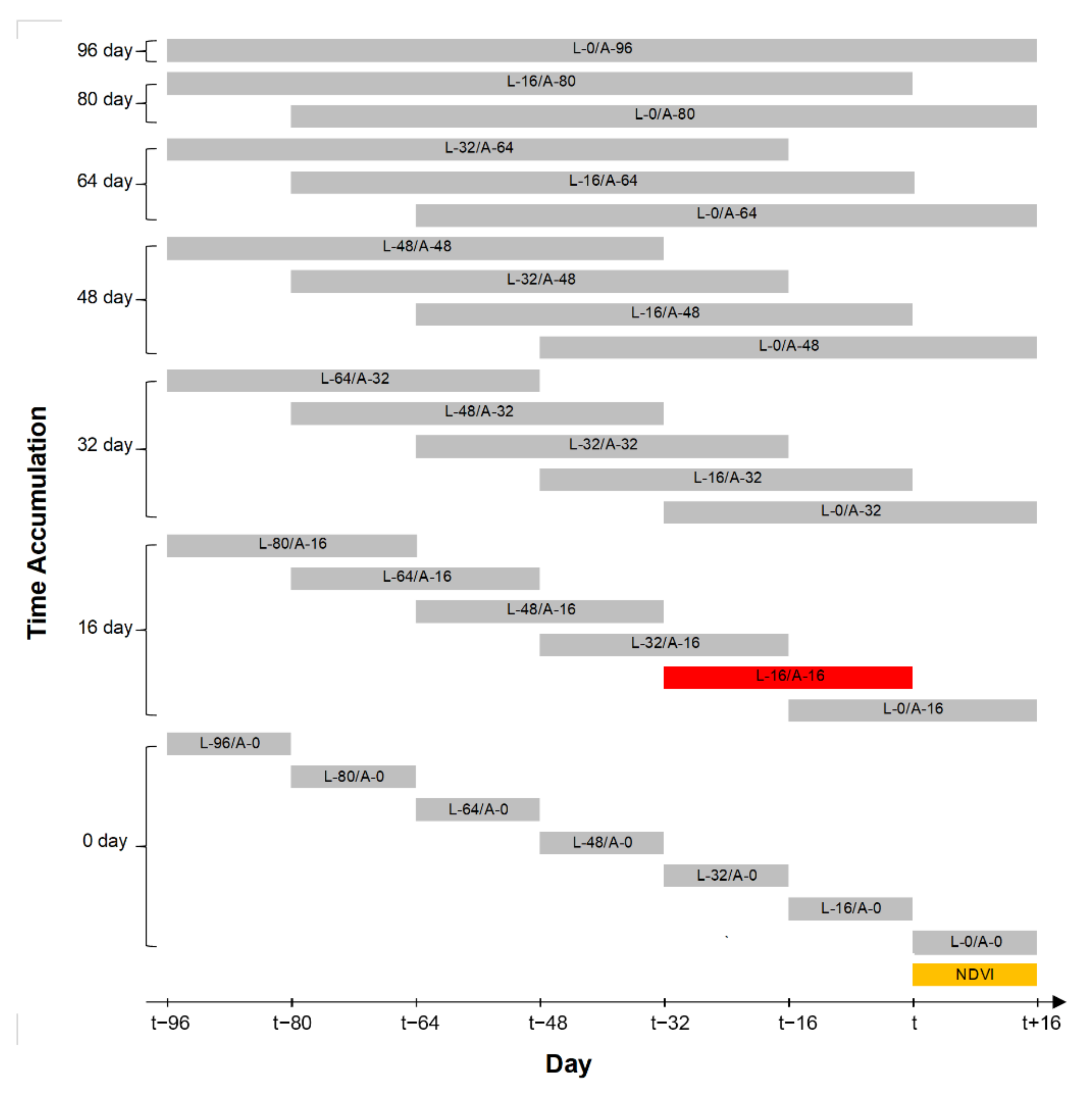
2.3.1. Trend Analysis and Partial Correlation Analysis

A simple linear regression model was used to analyze variations in the NDVI during the past 19 years, and the slope of the NDVI was calculated using the least-squares method:
Slope = n × i = 1 n i × NDVI i i = 1 n i i = 1 n NDVI i n × i = 1 n i 2 i = 1 n i 2
where NDVI i is the annual mean NDVI in the growing season in the ith year. A positive number indicates a trend of greening while a negative number indicates a browning trend. We used the F test (p < 0.05) to test significance [54,55].

2.3.2. Break Point Detection

We used the BFAST algorithm [27] in R language (https://cran.r-project.org/web/packages/bfast/index.html (accessed on 20 November 2019)) to explore shifts in the trend of the NDVI in the reserve. The algorithm is as follows:
Y t = T t + S t + e t ,   t = 1 , , n
This algorithm decomposes time series Y t (i.e., hydrology, climatology, and economics) during period t into trend ( T t ), seasonal ( S t ), and remainder components ( e t ); it then detects and characterizes abrupt changes in the time series. In our study, Y t denotes the 16-day NDVI time series in the growing season during 2000–2018.
We used BFAST01 implementation to detect either zero or one break point in the time series. Land use and land cover change are relative limited in our study area, and thus the detected break was likely to represent the most ecologically relevant shift in a time series [56]. We used the ordinary least-squares (OLS) residuals-based MOving-SUM (MOSUM) test [57] to evaluate whether break points occurred. We considered only points where both segments were significant (p < 0.05). According to de Jong et al. [58], six types of changes occur: monotonic greening, greening with setback, browning to greening, monotonic browning, browning with burst, and greening to browning.
We established buffer zones in ArcGIS software (version 10.3.1) to detect the influence of the natural reserve on the protection of vegetation. Considering the resolution of MODIS data and the previous research [12,59], the scope of the buffer zone was 25 km on both sides of the boundaries of the reserve, and we used the interval of 5 km when calculating variations in the NDVI. We did not conduct a buffer analysis of boundaries of the protected area that overlapped with national boundaries (Supplementary Information, Figure S2) because a large part of these buffer areas is in Nepal and have completely different vegetation types. Because we lacked a precise landcover product outside the QNNP, we masked pixels with an NDVI for the growing season of lower than 0.1 to minimize noise from ice, snow, water, sand, and stone when comparing variations in the NDVI between inside and outside the boundary of the reserve.

2.3.3. Factors Driving Changes in Vegetation

To analyze the impact of climate change on variations in the NDVI, we calculated the partial correlation coefficient (PCC) between the NDVI, and precipitation, temperature, and radiation. When calculating the association between the NDVI and a given factor, the two other factors were eliminated as control variables. The formula is as follows:
R 12 , 34 = R 12 , 3 R 14 , 3 × R 24 , 3 1 R 14 , 3 2 × 1 R 24 , 3 2
R 12 , 3 = R 12 R 13 × R 23 1 R 13 2 × 1 R 23 2
where R 12 , 34 is the partial correlation coefficient of variables 1 and 2, and variables 3 and 4 are the controlled variables, R 12 , 3 refers to the partial correlation coefficient of variables 1 and 2, and variable 2 is the controlled variable, and R 12 is the Pearson correlation coefficient of variables 1 and 2, and the other variables have similar meanings as before. The absolute value of the PCC is used to determine the best-fitting time effects. When calculating the PCC, the effects of time lag and time accumulation were considered. Previous work has shown that the time effects are generally shorter than a quarter of a year [60,61]. Therefore, we considered the effects of time lag and time accumulation up to a maximum of 96 days (approximately 3 months). Figure 2 shows the 28 schemes considered in this study. In Figure 2, NDVI(t,t+16) is the maximum NDVI value during the period (t~t+16). Take the scheme marked with red color (L-16/A-16) as an example, the corresponding climate factors are the accumulate values during the time periods (t−32~t).
To quantify the overall effect of climate change on variations in vegetation, a multiple linear regression model was developed:
NDVI = A × T M P + B × P R E + C × S R + ε
where A ,   B , and C are the regression coefficients, and ε is the error term. T M P ,   P R E , and S R are the adjusted time series of climatic factors (temperature, precipitation, and solar radiation, respectively) with the best effects of time lag and time accumulation identified through Equation (3). The absolute value of determination coefficient (R2) of Equation (5) was used to quantify the overall explanation of climatic factors for variations in the NDVI.

3. Results

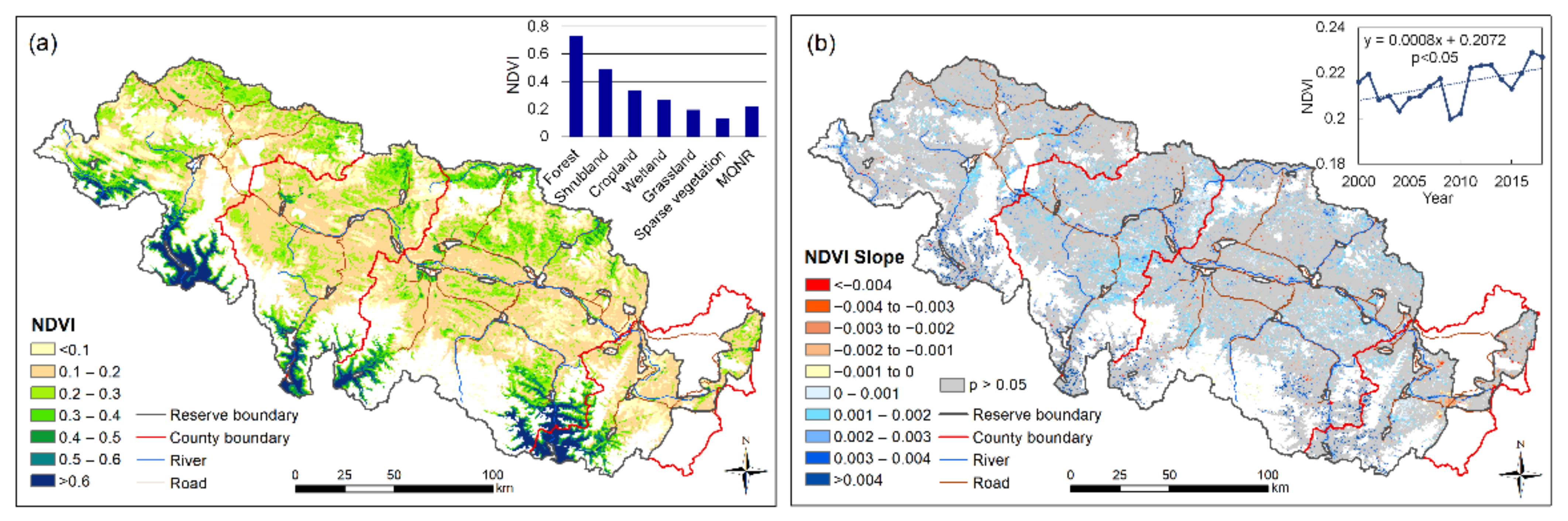
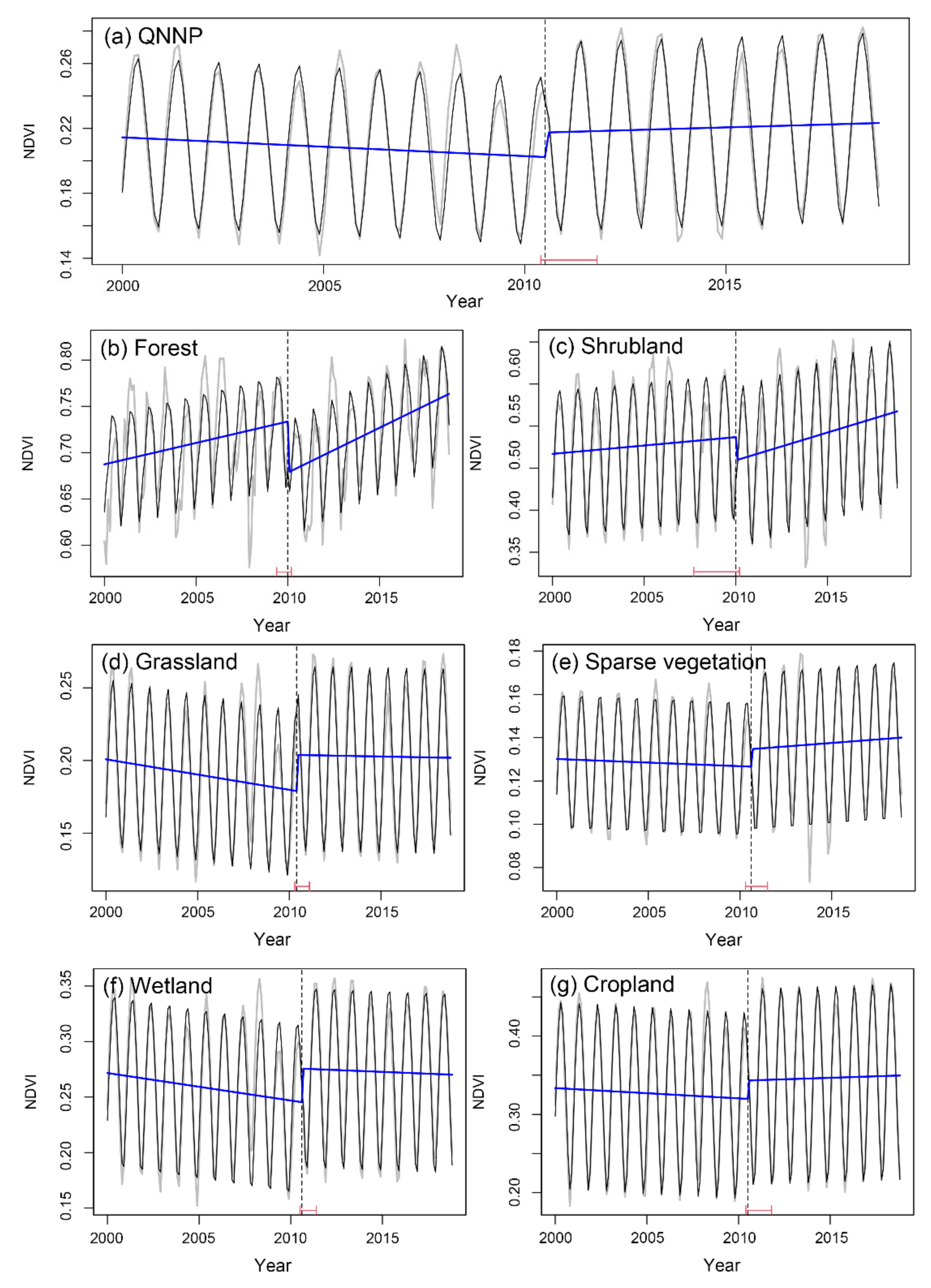
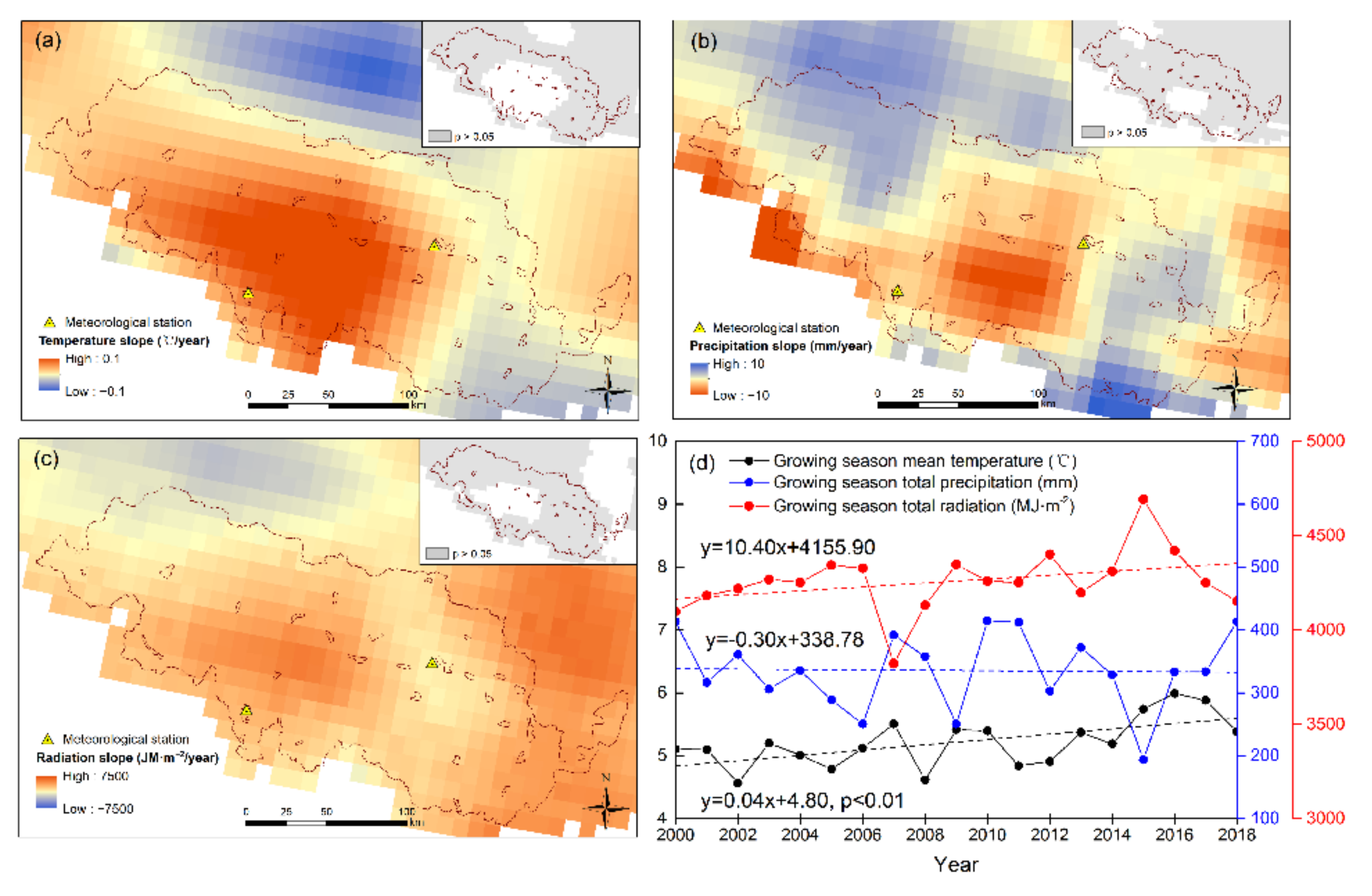
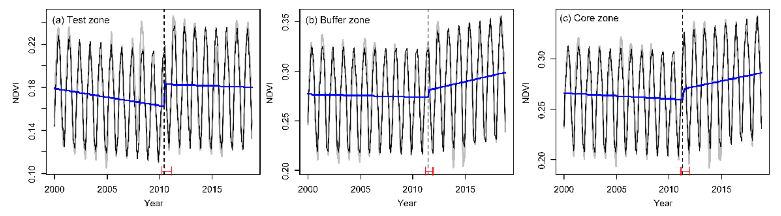
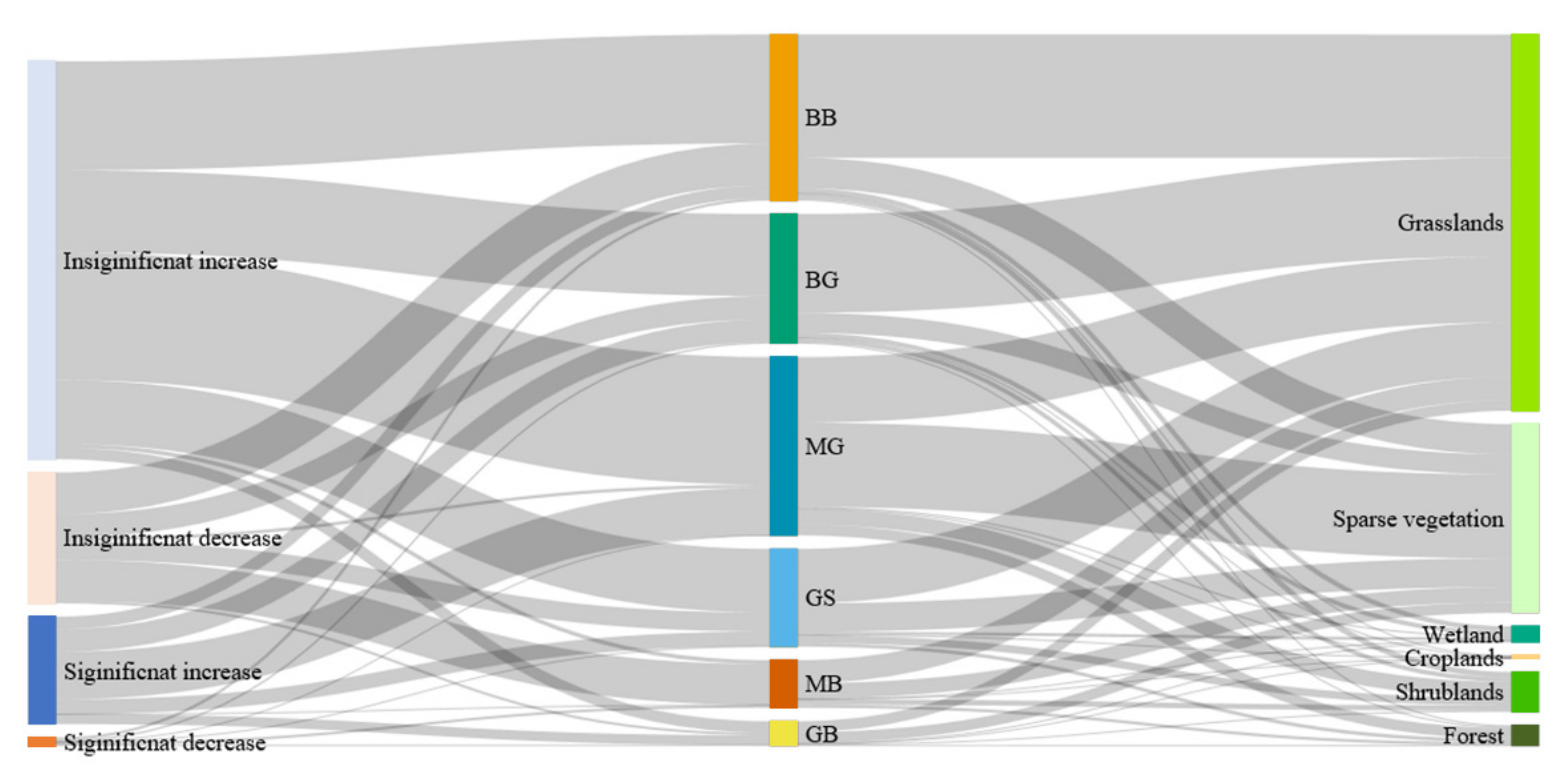
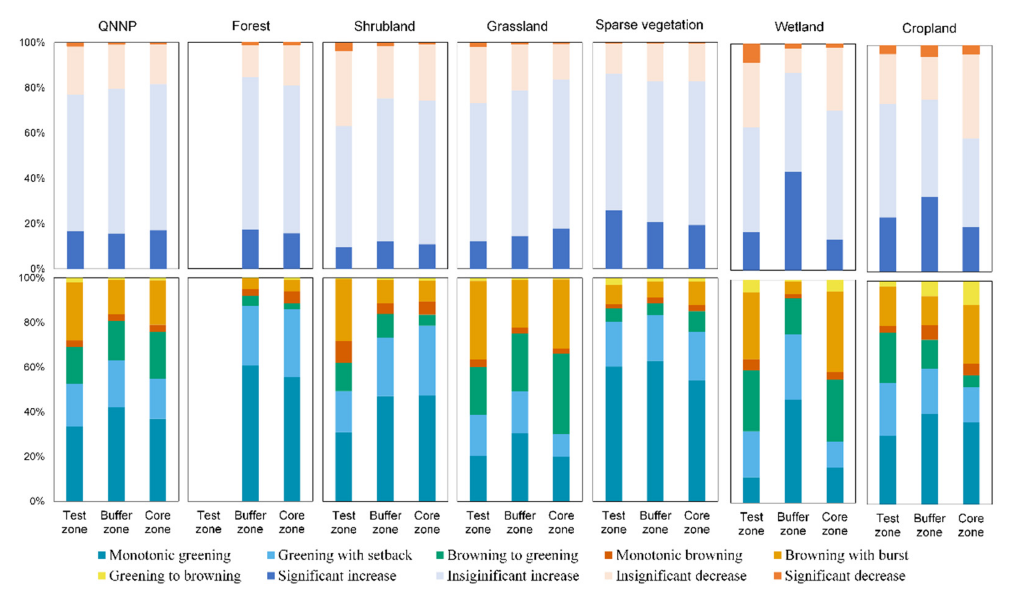
3.1. Spatial Distributions of Tendency and Shift in NDVI in QNNP in 2000–2018

The annual average NDVI exhibited large spatial heterogeneity in the QNNP (Figure 3a). Large NDVI values were mainly concentrated in the southern region of the preserve, where forests and shrubland dominated. The NDVI values below 0.3 were widely distributed in the middle region of the QNNP. Elevations in these regions were higher than the southern and northern regions, and they were mainly covered with grassland and sparse vegetation. Alongside the rivers, where wetlands dominate, the NDVI values were much higher than in the surroundings. For different vegetation types, forests had the largest NDVI (over 0.7), followed by shrubland and cropland; sparse vegetation and grassland had relatively low NDVI values. The annual mean NDVI in the QNNP generally showed a tendency of growth (0.0008 per year, p < 0.05) during 2000–2018. For the entire QNNP, vegetation with a significant and an insignificant trend of greening accounted for 16.66% and 61.77% of the total land, respectively (blue color in Figure 3b). Vegetation with a significant trend of decrease accounted for only 1.27% and was mainly concentrated in the east part of the region (Dinggye county) and the land alongside roads.
Using the BFAST model, we analyzed the shifts in the NDVI and their types (interruptions or reversals) in the QNPP during the past 19 years. Although the vegetation in the QNNP showed an overall tendency of growth, this overall period can be subdivided into two: 2000–2010, with an overall tendency of reduction (p < 0.05), and 2011–2018, with an overall tendency of increase (p < 0.05). Shift points in 2010 were also discovered for different vegetation types (Figure 4): After 2010, the tendencies of growth of forest and shrubland increased, the trend of cropland and sparse vegetation changed from one of decrease to that of increase, and the trends of decrease of wetland and grassland decreased compared with those in the first 10 years of the study period.
In terms of spatial distribution, the NDVI underwent significant shifts, accounting for 38.34% of the entire QNNP (Figure 5). A total of 29.24% of the shifts occurred during 2010–2011, and 15.57% in 2004. Among all the points with significant shifts, monotonic greening and greening with setback were widely distributed within the study area (green in Figure 5), accounting for 35.66% and 19.22%, respectively. The proportion of browning with burst (orange in Figure 5) was mainly distributed near rivers, roads, and the eastern region of Dinggye county. Notably, the reversal points, the points showing the transition from browning to greening (17.61%), accounted for much larger proportions of the QNNP than those representing the transition from greening to browning (1.72%). Points representing the transition from browning to greening were mainly distributed alongside rivers, lakes, and roads. Shifts from browning to greening mainly occurred before 2011 (90.38%), while a large number of shifts from greening to browning occurred after 2010 (85.11%).

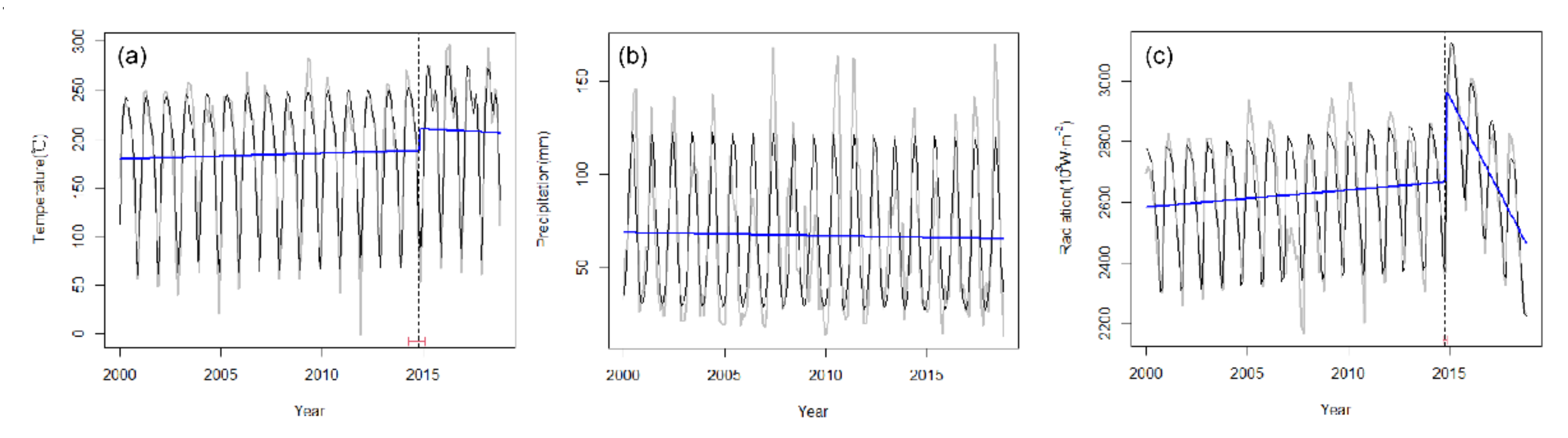
3.2. Climate Change and Its Impact on Variations in NDVI

To analyze the factors that might have affected the vegetation in the QNNP, we examined the response of the vegetation to the changing climate by considering the effects of time lag and time accumulation. We first analyzed the climatic trend of the QNNP during the study period (Figure 6). The entire QNNP exhibited a drying–warming trend in the growing season. During 2000–2018, most regions of the reserve showed a warming trend, especially the central part. Precipitation decreased significantly in the middle and southwest of the reserve and wetting in the northwestern and eastern parts of the reserve was insignificant. Radiation showed a trend of increase in the QNNP.
Time effects were examined by analyzing the PCC between the NDVI and climate variables over different periods (Table 1). The NDVI time series had the strongest PCC with temperature and precipitation at L-16/A-16 (cumulative over 16 days with 16 days of lag), and the maximum PCC values were 0.82 and 0.70, respectively. The response of the NDVI to radiation showed no time lag but a strong time accumulation effect (L-0/A-96, accumulated over 96 days with no day lag), and the maximum PCC was 0.70.
Figure 7a–c show the maximum PCC between the NDVI and the climate variables. The NDVI time series was significantly correlated with climatic factors across more than 90% of the vegetation area (p < 0.05). Temperature showed a 24.83 ± 20.44 (mean ± standard deviation)-day lag and a 11.35 ± 19.83-day accumulation at the regional scale. Grids without the time effect, with time lag, time accumulation, and their combined effects accounted for 8.01%, 57.93%, 15.81%, and 18.25% of the areas with significant vegetation, respectively (Figure 7d). In the south of the QNNP, the temperature showed a smaller time effect. Precipitation affected vegetation with an average lag of 17.38 ± 17.64 days and a 30.67 ± 28.42-day accumulation. The dominant time effect was the combined effect and time-accumulative effect, accounting for 52.99% and 29.49%, respectively (Figure 7e), of areas with significant vegetation. Radiation exhibited a 36.99 ± 41.93-day lag and 38.55 ± 39.09-day accumulation. The combined effect and that of time accumulation were the dominant effects of radiation, accounting for 46.20% and 27.84%, respectively (Figure 7f). Temperature and radiation generally had a larger impact than precipitation in the QNNP, as the absolute PCC values between the NDVI and precipitation were lower (Figure 7g). Considering the effects of time lag and time accumulation, a multiple linear regression model was established between the climate variables and the NDVI time series (Figure 7h). The result shows that the average explanatory power of the three climatic factors was 44.04% in the QNNP.
We used the data in Table 1 in the BFAST model to detect changes in the temperature and precipitation at L-16/A-16, and those in radiation at L-0/A-80 (Figure 8). We found no shifts in 2010, which does not help to explain the changes in the NDVI in this year. There were other reasons for variations in the NDVI in the QNNP.

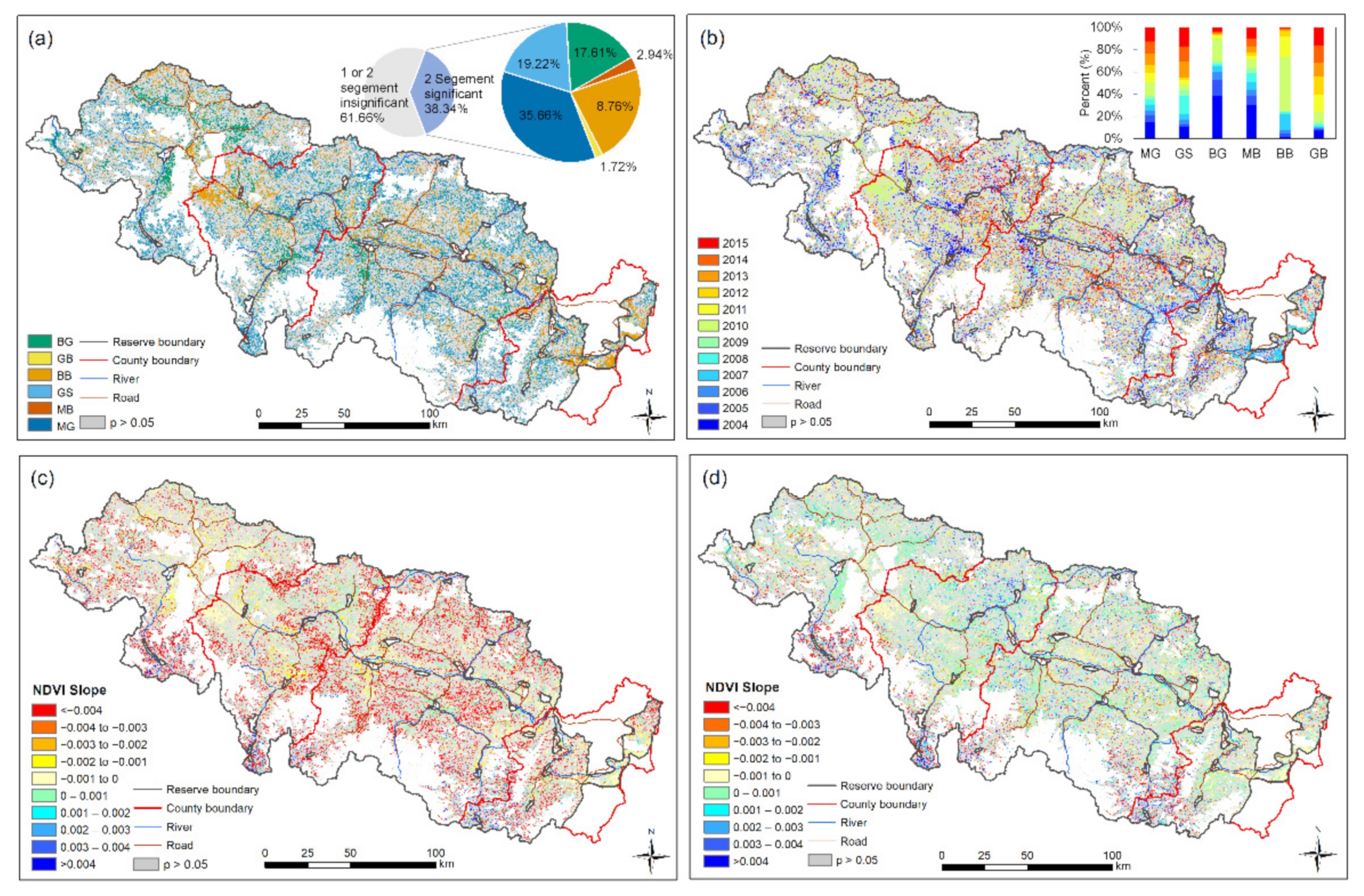
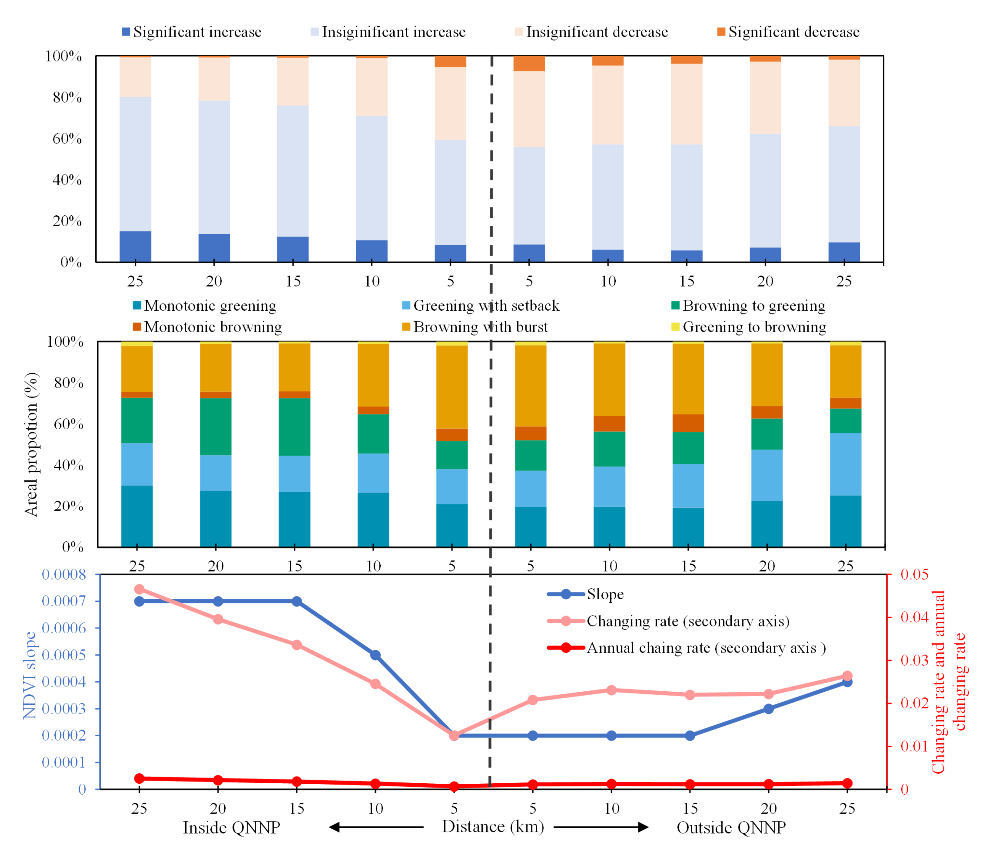
3.3. Impact of Human Activities on NDVI in QNNP

We first analyzed the variations in the NDVI in different zones of the QNNP to test the effectiveness of the protection of the reserve. The results showed that the tendencies of the growth of the vegetation in the core zone and the buffer zone were higher and more significant (p < 0.01) than those of the test zone (Table 2). The core zone had the highest annual rate of change (0.42%), and the buffer zone had the highest total rate of change. With regard to the shifts in the NDVI, the core zone and the buffer zone showed a trend from browning to greening while the test zone showed a decrease in vegetation with a positive break (Figure 9).
We further made buffers outside and inside the boundary of the reserve to study the differences between the variation in vegetation near the boundaries of the QNNP (Figure 10). Overall (in terms of all the indices), the vegetation growing inside the QNNP was generally better than that outside. The largest proportion of a significant decrease inside the QNNP was within 5 km of the border. With increasing distance, the proportion of significant/insignificant increases in the NDVI became larger closer to the core protected areas, as did the rate of change/annual rate of change in the NDVI. This characteristic was especially prominent for vegetation within 15 km of the border. In terms of shifts in the NDVI, the NDVI inside the reserve had larger proportions of monotonic greening areas and smaller proportions of monotonic browning and browning with burst. Compared with the area outside, a larger proportion of the vegetation inside the reserve had recovered, with trends of the NDVI shifting from that of decrease to one of increase.
We determined the variation in the livestock in the reserve because it feeds on plants and thus directly influences the vegetation and, in turn, the variations in the NDVI. As shown in Figure 11, the livestock number in the QNNP has increased drastically during 1952–2018. It was only 379,000 in 1952, while in 2008 it increased to more than 950,000. During our study period, the number of livestock showed a monotonic decrease in Tingri, and an increasing-to-decreasing trend in Dinggye and Gyirong. In Nyalam, the livestock slowly decreased and then increased in 2012. For the entire reserve, the livestock numbers showed a significant trend of decrease during 2010–2018 (Figure 11). This was consistent with the shift in the NDVI of the entire reserve in 2010.

4. Discussion

4.1. Variation in Vegetation in the Reserve

In the past 19 years, the NDVI in the reserve has shown a tendency of growth (0.0008/yr), which is also the case in the Koshi River Basin [62], the Himalayan region [6,39], and the TP [63,64]. Compared with past work that has focused on vegetation in the QNNP [40,41,42,43], we have specified variations in the NDVI after 2010, and find that the NDVI of the QNNP has not undergone a linear change. It changed from a trend of decrease to one of increase around 2010, which has not been reported for the reserve before. The patterns of the NDVI detected by BFAST in the first period were consistent with previous studies [40,42,44,65]. For instance, we found that forests and shrublands showed a trend of monotonic greening while the other vegetation types showed a trend of decrease in the first period. Nie et al. [42] also found that, during 1998–2009, forests and shrublands had a larger proportion of significant increase than significant decrease, whereas the proportions of significant increases in grassland, sparse vegetation, and croplands were smaller than the proportion of significant decreases. Ma et al. [65] found that during 2000–2009, the vegetation in the northern slopes mainly showed a trend of decrease, and over 40% of the vegetation showed different degrees of degradation. These places were dominated by grassland and sparse vegetation.
The BFAST can help detect shifts beyond the linear regression model and can provide more detail on the variations in the NDVI. Although the linear regression showed that all the vegetation types had exhibited tendencies of growth in the past 19 years (Table 2), grasslands and wetlands still need to be attended to. They showed a slight trend of decrease during 2010–2018 (Figure 4). Figure 12 shows that among the points of insignificant increase and significant increase, a large number of points exhibited browning with burst, and a greening-to-browning trend. Grassland and sparse vegetation accounted for large proportions of these two shift types. If protections are not reinforced in the future, the vegetation in these places will decrease in the long run.

4.2. Response of NDVI to Climatic Variables

Temperature and radiation were dominant among the climatic factors influencing the variations in the NDVI in the QNNP. This is consistent with a previous study that focused on the response of the NDVI to climatic factors in different regions of the TP [54] and other energy-limited middle-to-high latitudes of the Northern Hemisphere [60]. Increasing temperature and radiation are important factors for an increase in the greenness of the vegetation, and can significantly affect the vegetation of the TP, increase its productivity, height, and the duration of its growing periods [66,67,68]. The impact of radiation on the vegetation was not always positive. In the regions with limited water, high solar radiation increased the soil temperature, thus accelerating the transpiration of moisture and inhibiting vegetation growth [69,70]. Li et al. [55] found that in the southwestern TP, increasing temperature together with a growing amount of solar radiation adversely affected vegetation growth in the case of an insufficient supply of water. The effects of time lag and time accumulation were noted in the relationship between the NDVI and climatic variables in the QNNP and have been reported for the Yumco Basin [54], Naqu [71], and TP [72]. Plants need an accumulation of climatic factors to initiate their lifecycles and to obtain a sufficient amount of nutrients from the soil, heat, and moisture from the environment [60].
Climatic factors could explain 44.04% of the variations in the NDVI in the QNNP. This is below its global average value (63%) in a previous study [60]. This region is fragile to disturbances (i.e., over-grazing, land use changes, drought, fire, and plant diseases) [61]. In the context of shift detection, Li et al. [73] found adverse trends in precipitation in the entire southwestern TP and attributed the shift in the NDVI of the region to changing precipitation. However, in the QNNP we did not find any shift in climatic factors in 2010, and this cannot explain the shift in the NDVI in this year. Other factors should thus be taken into consideration in examining the variations in the NDVI in this region.

4.3. The Effectiveness of Conservation

The effectiveness of the natural reserve in the QNNP can be verified from the following: First, the buffer zone and the core zone generally had better vegetation conditions. The results showed that, since 2000, these zones had first decreased and then increased. The test zone showed a decrease in both periods, but after 2010 its rate of reduction decreased. Second, near the boundaries of the reserve, the vegetation inside the reserve generally grew better than that outside the boundary. Third, the result of the BFAST showed that 17.61% of the area had turned from brown to green and was not evenly distributed over the entire reserve but was mainly located alongside roads and rivers, or areas featuring intense human activities.
We further analyzed the tendencies of the NDVI for different types of vegetation in the three zones to confirm that the higher tendencies of NDVI growth in the buffer and core zones were caused by the establishment of different levels of protected zones, and not simply because the large areas of these zones were covered by forests and shrublands. The results showed that, except for the croplands (mainly located in the test zone), all types of vegetation had a higher tendency of growth, annual rate of change, and total rate of change in the buffer zone and the core zone than in the other zones (Table 2). In terms of the proportions of types of change (Figure 13), most vegetation had better growth conditions in the buffer and core zones. Land falling into categories of increase (significant/insignificant increase, monotonic greening, greening with setback, and browning to greening) generally constituted a higher proportion of land in these zones, with a higher proportion of land falling into categories of decrease (significant/insignificant decrease, monotonic browning, browning with burst, and greening to browning) in the test zone. Therefore, the core and buffer zones provided more effective protections than the test zone.
Previous studies also indicated the positive impact of the establishment of reserves in the TP. For instance, Zhang et al. [10] found that the NPP in 76% of samples inside nature reserves and 82% of samples inside national nature reserves in the TP was higher than that of the corresponding samples outside the reserve. Through comparing two reserves in the TP, Li et al. [74] found that longer-protected reserves exhibit higher stability to climate change. The establishment of natural reserves on the TP has reduced human activity [34]. According to the Chinese government’s regulations on nature reserves and the local policies, human activities (i.e., production facilities) were considerably restricted in the reserves, especially in the buffer zone and the core zone. Without permission, people are strictly prohibited to enter the core zone. While in the buffer zone, only non-destructive scientific research and observation are allowed. In the core zone and the buffer zone, no production facilities are allowed to be built. In the test zone, the production facilities cannot pollute the environment or destroy the landscapes. In the protected area, the core zone also constitutes areas featuring ecological engineering (i.e., the Natural Forest Protection Project, 1998, and the Green for Grain Project, 2002) [42].

4.4. The Impact of Livestock Decreasing

The policy-induced reduction of livestock could help to explain the NDVI increase in the reserve. Grazing has been practiced on the TP for three millennia [75]. However, during the past 50 years, due to the improved infrastructure, the growth of the population, and the market demand, grassland-livestock industry has quicky developed [76]. According to the study of Yu et al. [77], in 2010, the livestock number in the TP increased to nearly double the estimated capacity of all available pastures. Overgrazing is threatening the ecological security of the TP, becoming one of the major factors causing grassland degradation [78,79]. In our study area, during 1952–2008, the livestock number increased by 96.16%. This may cause a huge impact on the environment. Overgrazing can reduce the soil–water content, as well as nitrogen and phosphorus, causing a reduction in vegetation cover, vegetation height, and aboveground biomass [80], and changing the plant community structure (i.e., dominant species, richness, abundance, and life forms) [81]. Research on three regions of river sources has shown that increasing livestock numbers have eliminated the positive effect of climatic factors during 1984–1993 [82]. Field experiments have showed that it could influence the grassland to a greater extent than increasing temperature [83]. In the field experiment of Wang et al. [84], heavy grazing, rather than the warming climate, led to the degradation of alpine meadows.
We found that about 29.2% of the shifts occurred during 2010–2011, and the tendency of livestock growth in the reserve reversed around 2009 and has declined drastically since 2010. This variation is consistent with the implementation of engineering policies that have reduced livestock in Tibet. In 2011, the government reinforced the policy by introducing an award allowance payment policy, and has spent 1.6 million Yuan every year in pastoral areas of China to compensate for prohibitions on grazing, to reward efforts to achieve pasture–livestock equilibrium, and to provide production subsidies for herdsmen [85]. In addition, 15.57% of the shifts happened in 2004. The Chinese government enforced the ecological project, Grazing Withdraw Program (GWP), in 2003, bringing the implementation of many large-scale ecological projects, such as fencing degrading grassland, ecological compensation, and restoring the land cover vegetation [86]. The detection of the NDVI variation in the Qilian Mountain Region [21] also found positive abrupt change increased significantly since 2005, after the implementation of the GWP. Studies in the central TP found that the implement of ecological protection and restoration projects have mitigated grassland degradation, and even reversed the degradation in some areas [87]. Therefore, we thought that the policy-induced livestock decrease after 2010 might be one potential explanation for the NDVI shift in 2010.

4.5. Future Protection of Vegetation in the QNNP

The vegetation outside the reserve had a lower tendency of growth in the NDVI, and higher ratios of significant and insignificant trends of decrease. Human activity is one of the major factors leading to vegetation reduction near the boundaries. Li et al. [34] found that the human footprint has increased more significantly outside the QNNP reserve. Studies have also shown that the protected areas attract, rather than repel, human settlements by providing economic and occupational opportunities, and this threatens the effectiveness of conservation [88]. From Figure 11, we can see the population in the four counties showed a steady increase. Land cover changes may be another reason for a decrease in the NDVI [17]. The vegetation conditions outside the protected areas and the factors driving them should receive more attention because the environmental conditions and human activities in them can influence the natural resources within the reserves by affecting their biological and physical processes [8,89,90], and can create a ring of disturbance outside the reserve that isolates the protected area from its surroundings [81].
Apart from the overall tendencies of growth in the NDVI in the QNNP, reductions in it were observed in the wetlands at high altitudes and the forests alongside roads on the southern slope. We found a trend of decrease in wetlands during 2000–2010. A previous study has shown that during 2000–2008, degraded wetlands occupied 71.3 km2, or 1.8% of all wetlands in the QNNP [91]. The wetlands east of Dingye county underwent significant reductions in vegetation (red color in Figure 3). Such wetlands, especially flatlands along the riverbank, are perennially impacted by sand erosion [92]. In the valleys of the southern slopes, the destruction of forests, and the construction of roads and other infrastructure, together with frequent rainfall and unstable geological conditions, have triggered landslides, thus inflicting further damage on the surrounding vegetation. In addition, anthropogenic disturbances, i.e., fire, over-grazing, and lopping, hinder the natural succession of some species of trees by preventing the regeneration of seedlings and saplings from the understory of the forest [93].

4.6. Shortcomings of This Study

Our study gave a preliminary finding on the vegetation response and the impact from humans and the climate in the QNNP. The coarse resolution of the climate data could have affected the calculated variations in the vegetation due to climate change. In future work, weather stations in the surroundings could be gathered to generate more precise climate data.
With respect to the human influence, we considered only the livestock number in the region, while the surrounding industrial-scale activities (i.e., the construction of roads and built-up areas) could also bring impact on the environment. Although the impacted areas of those human activities are limited, mainly alongside the roads or surrounding the built-up areas, their influences are severe. However, the current study cannot differentiate the impacts from different human activities. In future studies, more human activities could be taken into consideration. Spatializing the statistical data can help to clarify the relevant influential factors in the different areas. Our work did not take the impact of the land use and the landcover change into consideration because it is difficult to capture by moderate resolution image. The applications of the satellite data with higher resolutions (i.e., Landsat, Sentinel) could help us to clarify the impact from the land use and the land cover change. In addition, more collaborative research involving the local stakeholders and researchers (i.e., a questionnaire survey in the local communities) could help us to better understand the influence of human activities in different scales, and make the study result more convincing [94].

5. Conclusions

We studied the variations in the NDVI of the QNNP during 2000–2018 in this paper. We applied the break point detection to monitor variations in the vegetation in the protected areas. This algorithm can help provide detailed information on the changes in the vegetation so to implement timely protection measures. The results showed that the vegetation in the reserve had grown during the past 19 years, but its growth was not monotonic. The vegetation declined in the first 10 years, and then grew after 2010.
We found that climatic factors could account for only 40.04% of the variation in the vegetation in the QNNP. Human activity has thus affected the vegetation in even the highest region of the world. Although the linear regression model showed that all vegetation types had an increasing tendency, the result of the BFAST algorithm showed that grasslands and wetlands had decreased after 2010. The vegetation in the test zone, especially near the boundary of the reserve, should be strictly protected. Our work here can provide information for the sustainable management of the reserve.

Supplementary Materials

The following are available online at https://0-www-mdpi-com.brum.beds.ac.uk/article/10.3390/rs13224725/s1, Figure S1: Comparison of the ground-observed climate data and the China Meteorological Forcing Dataset. Figure S2: NDVI trends around the reserve boundary. Insert figures is NDVI trends with p value higher than 0.05 being masked out.

Author Contributions

Conceptualization, funding acquisition, project administration, supervision; Y.Z.; Data curation, formal analysis, visualization, writing—original draft, B.Z.; Methodology, software, B.Z., L.L. (Lanhui Li) and H.Z.; Writing—review and editing, Z.W., M.D., L.L. (Linshan Liu), L.L. (Lanhui Li), S.L., Q.L. and B.P. All authors have read and agreed to the published version of the manuscript.

Funding

This study was funded by the Second Tibetan Plateau Scientific Expedition and Research (Grant No. 2019QZKK0603), the Strategic Priority Research Program of the Chinese Academy of Sciences (Grant No. XDA20040201), the National Natural Science Foundation of China (Grant No. 41761144081), and the Chinese Academy of Sciences President’s International Fellowship Initiative for postdoctoral research (2018PC0030).

Institutional Review Board Statement

Not applicable.

Informed Consent Statement

Not applicable.

Data Availability Statement

Data used in this study will be available upon request from the first author.

Acknowledgments

We thank Yong Nie for providing the land use/land cover data for the QNNP. We thank Bo Wei for providing help in coding. We are grateful to the group members who spent time on field work in the QNNP. We are also grateful to the anonymous reviewers for providing useful suggestions to improve the manuscript.

Conflicts of Interest

The authors declare no conflict of interest.

References

  1. Margules, C.R.; Pressey, R.L. Systematic conservation planning. Nature 2000, 405, 243–253. [Google Scholar] [CrossRef] [PubMed]
  2. Kolahi, M.; Sakai, T.; Moriya, K.; Makhdoum, M.F.; Koyama, L. Assessment of the effectiveness of protected areas management in Iran: Case study in Khojir national park. Environ. Manag. 2013, 52, 514–530. [Google Scholar] [CrossRef]
  3. UNEP-WCMC; IUCN; NGS. Protected Planet Report 2018; UNEP-WCMC: Cambridge, UK; IUCN: Gland, Switzerland; NGS: Washington, DC, USA, 2018; pp. 5–6. [Google Scholar]
  4. Leverington, F.; Costa, K.L.; Pavese, H.; Lisle, A.; Hockings, M. A global analysis of protected area management effectiveness. Environ. Manag. 2010, 46, 685–698. [Google Scholar] [CrossRef]
  5. Laurance, W.F.; Carolina Useche, D.; Rendeiro, J.; Kalka, M.; Bradshaw, C.J.A.; Sloan, S.P.; Laurance, S.G.; Campbell, M.; Abernethy, K.; Alvarez, P.; et al. Averting biodiversity collapse in tropical forest protected areas. Nature 2012, 489, 290–294. [Google Scholar] [CrossRef] [Green Version]
  6. Mishra, N.B.; Mainali, K.P. Greening and browning of the Himalaya: Spatial patterns and the role of climatic change and human drivers. Sci. Total Environ. 2017, 587–588, 326–339. [Google Scholar] [CrossRef] [PubMed]
  7. Tegler, B.; Sharp, M.; Johnson, M.A. Ecological monitoring and assessment network’s proposed core monitoring variables: An early warning of environmental change. Environ. Monit. Assess. 2001, 67, 29–56. [Google Scholar] [CrossRef] [PubMed]
  8. Townsend, P.A.; Lookingbill, T.R.; Kingdon, C.C.; Gardner, R.H. Spatial pattern analysis Protected Planet Report 2018 for monitoring protected areas. Remote Sens. Environ. 2009, 113, 1410–1420. [Google Scholar] [CrossRef]
  9. Tang, Z.; Fang, J.; Sun, J.; Gaston, K.J. Effectiveness of protected areas in maintaining plant production. PLoS ONE 2011, 6, e99116. [Google Scholar] [CrossRef]
  10. Zhang, Y.; Hu, Z.; Qi, W.; Wu, X.; Bai, W.; Li, L.; Ding, M.; Liu, L.; Wang, Z.; Zheng, D. Assessment of protection effectiveness of nature reserves on the Tibetan Plateau based on net primary production and the large-sample-comparison method. Acta Geogr. Sin. 2015, 70, 1027–1040. [Google Scholar]
  11. Huang, C.; Goward, S.N.; Schleeweis, K.; Thomas, N.; Masek, J.G.; Zhu, Z. Dynamics of national forests assessed using the Landsat record: Case studies in eastern United States. Remote Sens. Environ. 2009, 113, 1430–1442. [Google Scholar] [CrossRef]
  12. Brink, A.B.; Martínez-López, J.; Szantoi, Z.; Moreno-Atencia, P.; Lupi, A.; Bastin, L.; Dubois, G. Indicators for assessing habitat values and pressures for protected areas—An integrated habitat and land cover change approach for the Udzungwa mountains national park in Tanzania. Remote Sens. 2016, 8, 862. [Google Scholar] [CrossRef] [Green Version]
  13. Rouse, J.R.; Haas, R.H.; Schell, J.A.; Deering, D.W. Monitoring the vernal advancement and retrogradation (green wave effect) of natural vegetation. In NASA/GFSC Type III Final Report; NASA: Greenbelt, MD, USA, 1974. [Google Scholar]
  14. Huete, A.; Didan, K.; Miura, T.; Rodriguez, E.P.; Gao, X.; Ferreira, L.G. Overview of the radiometric and biophysical performance of the MODIS vegetation indices. Remote Sens. Environ. 2002, 83, 195–213. [Google Scholar] [CrossRef]
  15. Alcaraz-Segura, D.; Cabello, J.; Paruelo, J.M.; Delibes, M. Use of descriptors of ecosystem functioning for monitoring a national park network: A remote sensing approach. Environ. Manag. 2009, 43, 38–48. [Google Scholar] [CrossRef]
  16. Nemani, R.; Hashimoto, H.; Votava, P.; Melton, F.; Wang, W.; Michaelis, A.; Mutch, L.; Milesi, C.; Hiatt, S.; White, M. Monitoring and forecasting ecosystem dynamics using the Terrestrial Observation and Prediction System (TOPS). Remote Sens. Environ. 2009, 113, 1497–1509. [Google Scholar] [CrossRef]
  17. Zeng, J.; Chen, T.; Yao, X.; Chen, W. Do Protected Areas Improve Ecosystem Services? A Case Study of Hoh Xil Nature Reserve in Qinghai-Tibetan Plateau. Remote Sens. 2020, 12, 471. [Google Scholar] [CrossRef] [Green Version]
  18. Duran, A.P.; Casalegno, S.; Marquet, P.A.; Gaston, K.J. Representation of Ecosystem Services by Terrestrial Protected Areas: Chile as a Case Study. PLoS ONE 2013, 8, e82643. [Google Scholar]
  19. Zhang, Y.; Peng, C.; Li, W.; Tian, L.; Zhu, Q.; Chen, H.; Fang, X.; Zhang, G.; Liu, G.; Mu, X.; et al. Multiple afforestation programs accelerate the greenness in the ‘Three North’ region of China from 1982 to 2013. Ecol. Indic. 2016, 61, 404–412. [Google Scholar] [CrossRef]
  20. Liu, M.; Dries, L.; Heijman, W.; Huang, J.; Zhu, X.; Hu, Y.; Chen, H. The Impact of Ecological Construction Programs on Grassland Conservation in Inner Mongolia, China. Land Degrad. Dev. 2018, 29, 326–336. [Google Scholar] [CrossRef] [Green Version]
  21. Geng, L.; Che, T.; Wang, X.; Wang, H. Detecting Spatiotemporal Changes in Vegetation with the BFAST Model in the Qilian Mountain Region during 2000–2017. Remote Sens. 2019, 11, 103. [Google Scholar] [CrossRef] [Green Version]
  22. Verbesselt, J.; Hyndman, R.; Zeileis, A.; Culvenor, D. Phenological change detection while accounting for abrupt and gradual trends in satellite image time series. Remote Sens. Environ. 2010, 114, 2970–2980. [Google Scholar] [CrossRef] [Green Version]
  23. Huang, C.; Goward, S.N.; Masek, J.G.; Thomas, N.; Zhu, Z.; Vogelmann, J.E. An automated approach for reconstructing recent forest disturbance history using dense Landsat time series stacks. Remote Sens. Environ. 2010, 114, 183–198. [Google Scholar] [CrossRef]
  24. Kennedy, R.E.; Yang, Z.; Cohen, W.B. Detecting trends in forest disturbance and recovery using yearly Landsat time series: 1. LandTrendr—Temporal segmentation algorithms. Remote Sens. Environ. 2010, 114, 2897–2910. [Google Scholar] [CrossRef]
  25. Zhu, Z.; Woodcock, C.E. Continuous change detection and classification of land cover using all available Landsat data. Remote Sens. Environ. 2014, 144, 152–171. [Google Scholar] [CrossRef] [Green Version]
  26. Jamali, S.; Jönsson, P.; Eklundh, L.; Ardö, J.; Seaquist, J. Detecting changes in vegetation trends using time series segmentation. Remote Sens. Environ. 2015, 156, 182–195. [Google Scholar] [CrossRef]
  27. Verbesselt, J.; Hyndman, R.; Newnham, G.; Culvenor, D. Detecting trend and seasonal changes in satellite image time series. Remote Sens. Environ. 2010, 114, 106–115. [Google Scholar] [CrossRef]
  28. Watts, L.M.; Laffan, S.W. Effectiveness of the BFAST algorithm for detecting vegetation response patterns in a semi-arid region. Remote Sens. Environ. 2014, 154, 234–245. [Google Scholar] [CrossRef]
  29. Saatchi, S.; Asefi-Najafabady, S.; Malhi, Y.; Aragao, L.E.O.C.; Anderson, L.O.; Myneni, R.B.; Nemani, R. Persistent effects of a severe drought on Amazonian forest canopy. Proc. Natl. Acad. Sci. USA 2013, 110, 565–570. [Google Scholar] [CrossRef] [Green Version]
  30. Fang, X.; Zhu, Q.; Ren, L.; Chen, H.; Wang, K.; Peng, C. Large-scale detection of vegetation dynamics and their potential drivers using MODIS images and BFAST: A case study in Quebec, Canada. Remote Sens. Environ. 2018, 206, 391–402. [Google Scholar] [CrossRef]
  31. Devries, B.; Verbesselt, J.; Kooistra, L.; Herold, M. Robust monitoring of small-scale forest disturbances in a tropical montane forest using Landsat time series. Remote Sens. Environ. 2015, 161, 107–121. [Google Scholar] [CrossRef]
  32. Sun, H.; Zheng, D.; Yao, T.; Zhang, Y. Protection and construction of the national ecological security shelter zone on Tibetan Plateau. Acta Geogr. Sin. 2012, 67, 3–12. [Google Scholar]
  33. Zhang, D.; Huang, J.; Guan, X.; Chen, B.; Zhang, L. Long-term trends of precipitable water and precipitation over the Tibetan Plateau derived from satellite and surface measurements. J. Quant. Spectrosc. Radiat. Transf. 2013, 122, 64–71. [Google Scholar] [CrossRef]
  34. Li, S.; Wu, J.; Gong, J.; Li, S. Human footprint in Tibet: Assessing the spatial layout and effectiveness of nature reserves. Sci. Total Environ. 2018, 621, 18–29. [Google Scholar] [CrossRef]
  35. Zhang, Y.; Wu, X.; Qi, W.; Li, S.; Bai, W. Characteristics and protection effectiveness of nature reserves on the Tibetan Plateau, China. Resour. Sci. 2015, 37, 1455–1464. [Google Scholar]
  36. Tsetan, L. Overview of mount Qomolangma nature reserve. China Tibetol. 1997, 10, 3–22. [Google Scholar]
  37. Ramachandran, R.M.; Roy, P.S. Vegetation response to climate change in Himalayan hill ranges: A remote sensing perspective. Plant Divers. Himalaya Hotspot Reg. 2018, I, 369–392. [Google Scholar]
  38. Li, B. A preliminary evaluation of the mount Qomolangma nature reserve. J. Nat. Resour. 1993, 8, 97–104. [Google Scholar]
  39. Anderson, K.; Fawcett, D.; Cugulliere, A.; Benford, S.; Jones, D.; Leng, R. Vegetation expansion in the subnival Hindu Kush Himalaya. Glob. Chang. Biol. 2020, 26, 1608–1625. [Google Scholar] [CrossRef] [Green Version]
  40. Kan, A.; Wang, X.; Gao, Z.; Li, G.; Luo, Y. Vegetation spatio-temporal changes and driving factors in the Mt. Qomolangma nature reserve in 2000–2007. Ecol. Environ. Sci. 2010, 19, 1261–1271. [Google Scholar]
  41. Chen, Y. A Research into Vegetation Changes of the Mt. Qomolangma National Nature Reserve. Master’s Thesis, Chengdu University of Technology, Chengdu, China, 2012. [Google Scholar]
  42. Nie, Y.; Liu, L.; Zhang, Y.; Ding, M. NDVI change analysis in the mount Qomolangma (Everest) national nature preserve during 1982–2009. Prog. Geogr. 2012, 31, 895–903. [Google Scholar]
  43. Zhang, W.; Zhang, Y.; Wang, Z.; Ding, M.; Yang, X.; Lin, X.; Yan, Y. Analysis of vegetation change in Mt. Qomolangma nature reserve. Prog. Geogr. 2006, 25, 12–21+137. [Google Scholar]
  44. Zhang, W.; Zhang, Y.; Wang, Z.; Ding, M.; Yang, X.; Lin, X.; Liu, L. Vegetation change in the Mt. Qomolangma Nature Reserve from 1981 to 2001. J. Geogr. Sci. 2007, 17, 152–164. [Google Scholar] [CrossRef]
  45. Ma, F.; Kan, A.; Li, J.; Guan, L.; Chen, X. Distribution and potential degradation risk evaluation of marsh wetland in the Mt. Qomolangma national nature reserve. J. Geo-Inf. Sci. 2011, 13, 594–600. [Google Scholar] [CrossRef]
  46. Zhang, Y.; Li, B.; Liu, L.; Zheng, D. Redetermine the region and boundaries of Tibetan Plateau. Geogr. Res. 2021, 40, 1543–1553. [Google Scholar]
  47. Nie, Y. Land Cover Changes in Mt. Qomolangma Region. Ph.D. Thesis, Chinese Academy of Science, Beijing, China, 2010. [Google Scholar]
  48. Jönsson, P.; Eklundh, L. TIMESAT—A program for analyzing time-series of satellite sensor data. Comput. Geosci. 2004, 30, 833–845. [Google Scholar] [CrossRef] [Green Version]
  49. Yuan, H.; Dai, Y.; Xiao, Z.; Ji, D.; Wei, S. Reprocessing the MODIS Leaf Area Index products for land surface and climate modelling. Remote Sens. Environ. 2011, 115, 1171–1187. [Google Scholar] [CrossRef]
  50. Alcantara, C.; Kuemmerle, T.; Prishchepov, A.V.; Radeloff, V.C. Mapping abandoned agriculture with multi-temporal MODIS satellite data. Remote Sens. Environ. 2012, 124, 334–347. [Google Scholar] [CrossRef]
  51. Savitzky, A.; Golay, M.J.E. Smoothing and differentiation of data by simplified least squares procedures. Anal. Chem. 1964, 36, 1627–1639. [Google Scholar] [CrossRef]
  52. Zhang, Y.; Liu, L.; Nie, Y.; Zhang, J.; Zhang, X. Land Cover Mapping in the Qomolangma (Everest) National Nature Preserve. In Land Use & Land Cover Change and the Climate Change Adaptation in Tibetan Plateau; Zhang, Y., Ed.; China Meteorological Press: Beijing, China, 2012; pp. 129–158. [Google Scholar]
  53. He, J.; Yang, K.; Tang, W.; Lu, H.; Qin, J.; Chen, Y.; Li, X. The first high-resolution meteorological forcing dataset for land process studies over China. Sci. Data 2020, 7, 25. [Google Scholar] [CrossRef] [Green Version]
  54. Zhe, M.; Zhang, X. Time-lag effects of NDVI responses to climate change in the Yamzhog Yumco Basin, South Tibet. Ecol. Indic. 2021, 124, 107431. [Google Scholar] [CrossRef]
  55. Li, L.; Zhang, Y.; Liu, L.; Wu, J.; Wang, Z.; Li, S.; Zhang, H.; Zu, J.; Ding, M.; Paudel, B. Spatiotemporal patterns of vegetation greenness change and associated climatic and anthropogenic drivers on the Tibetan Plateau during 2000–2015. Remote Sens. 2018, 10, 1525. [Google Scholar] [CrossRef] [Green Version]
  56. Horion, S.; Prishchepov, A.V.; Verbesselt, J.; de Beurs, K.; Tagesson, T.; Fensholt, R. Revealing turning points in ecosystem functioning over the Northern Eurasian agricultural frontier. Glob. Chang. Biol. 2016, 22, 2801–2817. [Google Scholar] [CrossRef]
  57. Chu, C.J.; Homik, K.; Kuan, C. MOSUM tests for parameter constancy. Biometrika 1995, 82, 603–617. [Google Scholar] [CrossRef]
  58. De Jong, R.; Verbesselt, J.; Zeileis, A.; Schaepman, M.E. Shifts in global vegetation activity trends. Remote Sens. 2013, 5, 1117. [Google Scholar] [CrossRef] [Green Version]
  59. Bailey, K.M.; Mccleery, R.A.; Binford, M.W.; Zweig, C. Land-cover change within and around protected areas in a biodiversity hotspot. J. Land Use Sci. 2016, 11, 154–176. [Google Scholar] [CrossRef]
  60. Ding, Y.; Li, Z.; Peng, S. Global analysis of time-lag and -accumulation effects of climate on vegetation growth. Int. J. Appl. Earth Obs. Geoinf. 2020, 92, 102179. [Google Scholar] [CrossRef]
  61. Wu, D.; Zhao, X.; Liang, S.; Zhou, T.; Huang, K.; Tang, B.; Zhao, W. Time-lag effects of global vegetation responses to climate change. Glob. Chang. Biol. 2015, 21, 3520–3531. [Google Scholar] [CrossRef]
  62. Zhang, Y.; Gao, J.; Liu, L.; Wang, Z.; Ding, M.; Yang, X. NDVI-based vegetation changes and their responses to climate change from 1982 to 2011: A case study in the Koshi River Basin in the middle Himalayas. Glob. Planet. Chang. 2013, 108, 139–148. [Google Scholar] [CrossRef]
  63. Zhang, Y.; Liu, L.; Wang, Z.; Bai, W.; Ding, M.; Wang, X.; Yan, J.; Xu, E.; Wu, X.; Zhang, B.; et al. Spatial and temporal characteristics of land use and cover changes in the Tibetan Plateau. Chin. Sci. Bull. 2019, 64, 2865–2875. [Google Scholar]
  64. Li, L.; Zhang, Y.; Wu, J.; Li, S.; Zhang, B.; Zu, J.; Zhang, H.; Ding, M.; Paudel, B. Increasing sensitivity of alpine grasslands to climate variability along an elevational gradient on the Qinghai-Tibet Plateau. Sci. Total Environ. 2019, 678, 21–29. [Google Scholar] [CrossRef]
  65. Ma, F.; Li, J.; Peng, P.; Gao, Z.; Kan, A. Vegetation changes on Southern and Northern slopes of the Mt. Qomolangma National Nature Reserve. Prog. Geogr. 2010, 29, 1427–1432. [Google Scholar]
  66. Gao, Y.; Zhou, X.; Wang, Q.; Wang, C.; Zhan, Z.; Chen, L.; Yan, J.; Qu, R. Vegetation net primary productivity and its response to climate change during 2001–2008 in the Tibetan Plateau. Sci. Total Environ. 2013, 444, 356–362. [Google Scholar] [CrossRef] [PubMed]
  67. Shen, M.; Piao, S.; Chen, X.; An, S.; Fu, Y.H.; Wang, S.; Cong, N.; Janssens, I.A. Strong impacts of daily minimum temperature on the green-up date and summer greenness of the Tibetan Plateau. Glob. Chang. Biol. 2016, 22, 3057–3066. [Google Scholar] [CrossRef] [PubMed]
  68. Zhu, Z.; Piao, S.; Myneni, R.B.; Huang, M.; Zeng, Z.; Canadell, J.G.; Ciais, P.; Sitch, S.; Friedlingstein, P.; Arneth, A.; et al. Greening of the Earth and its drivers. Nat. Clim. Chang. 2016, 6, 791–795. [Google Scholar] [CrossRef]
  69. An, S.; Zhu, X.; Shen, M.; Wang, Y.; Cao, R.; Chen, X.; Yang, W.; Chen, J.; Tang, Y. Mismatch in elevational shifts between satellite observed vegetation greenness and temperature isolines during 2000–2016 on the Tibetan Plateau. Glob. Chang. Biol. 2018, 24, 5411–5425. [Google Scholar] [CrossRef] [PubMed]
  70. Liang, E.; Leuschner, C.; Dulamsuren, C.; Wagner, B.; Hauck, M. Global warming-related tree growth decline and mortality on the north-eastern Tibetan plateau. Clim. Chang. 2016, 134, 163–176. [Google Scholar] [CrossRef]
  71. Shen, B.; Fang, S.; Li, G. Vegetation Coverage Changes and Their Response to Meteorological Variables from 2000 to 2009 in Naqu, Tibet, China. Can. J. Remote Sens. 2014, 40, 67–74. [Google Scholar] [CrossRef]
  72. Chen, J.; Yan, F.; Lu, Q. Spatiotemporal Variation of Vegetation on the Qinghai–Tibet Plateau and the Influence of Climatic Factors and Human Activities on Vegetation Trend (2000–2019). Remote Sens. 2020, 12, 3150. [Google Scholar] [CrossRef]
  73. Li, P.; Hu, Z.; Liu, Y. Shift in the trend of browning in Southwestern Tibetan Plateau in the past two decades. Agric. For. Meteorol. 2020, 287, 107950. [Google Scholar] [CrossRef]
  74. Li, J.; Cong, N.; Zu, J.; Xin, Y.; Huang, K.; Zhou, Q.; Liu, Y.; Zhou, L.; Wang, L.; Liu, Y.; et al. Longer conserved alpine forests ecosystem exhibits higher stability to climate change on the Tibetan Plateau. J. Plant Ecol. 2019, 12, 645–652. [Google Scholar] [CrossRef]
  75. Long, R.J. Alpine rangeland ecosystem and their management in the Qinghai-Tibetan plateau. In The Yak, 2nd ed.; Wiener, G., Han, J.L., Long, R.J., Eds.; FAO Regional Office for Asia and the Pacific: Bangkok, Thailand, 2003; pp. 359–388. [Google Scholar]
  76. Shang, Z.H.; Gibb, M.J.; Leiber, F.; Ismail, M.; Ding, L.M.; Guo, X.S.; Long, R.J. The sustainable development of grassland-livestock systems on the Tibetan plateau: Problems, strategies and prospects. Rangel. J. 2014, 36, 267–296. [Google Scholar] [CrossRef] [Green Version]
  77. Yu, C.; Zhang, Y.; Claus, H.; Zeng, R.; Zhang, X.; Wang, J. Ecological and Environmental Issues Faced by a Developing Tibet. Environ. Sci. Technol. 2012, 46, 1979–1980. [Google Scholar] [CrossRef] [PubMed]
  78. Harris, R.B. Rangeland degradation on the Qinghai-Tibetan plateau: A review of the evidence of its magnitude and causes. J. Arid. Environ. 2010, 74, 1–12. [Google Scholar] [CrossRef]
  79. Sun, J.; Liu, M.; Fu, B.; Kemp, D.; Zhao, W.; Liu, G.; Han, G.; Wilkes, A.; Lu, X.; Chen, Y.; et al. Reconsidering the efficiency of grazing exclusion using fences on the Tibetan Plateau. Sci. Bull. 2020, 65, 1405–1414. [Google Scholar] [CrossRef]
  80. Li, W.; Cao, W.; Wang, J.; Li, X.; Xu, C.; Shi, S. Effects of grazing regime on vegetation structure, productivity, soil quality, carbon and nitrogen storage of alpine meadow on the Qinghai-Tibetan Plateau. Ecol. Eng. 2017, 98, 123–133. [Google Scholar] [CrossRef]
  81. Niu, Y.; Yang, S.; Wang, G.; Liu, L.; Hua, L. Effects of grazing disturbance on plant diversity, community structure and direction of succession in an alpine meadow on Tibet Plateau, China. Acta Ecol. Sin. 2018, 38, 274–280. [Google Scholar] [CrossRef]
  82. Lu, Q.; Ning, J.; Liang, F.; Bi, X. Evaluating the effects of government policy and drought from 1984 to 2009 on rangeland in the Three Rivers Source region of the Qinghai-Tibet Plateau. Sustainability 2017, 9, 1033. [Google Scholar] [CrossRef] [Green Version]
  83. Zhang, Y.; Gao, Q.; Dong, S.; Liu, S.; Wang, X.; Su, X.; Li, Y.; Tang, L.; Wu, X.; Zhao, H. Effects of grazing and climate warming on plant diversity, productivity and living state in the alpine rangelands and cultivated grasslands of the Qinghai-Tibetan Plateau. Rangel. J. 2015, 37, 57–65. [Google Scholar] [CrossRef]
  84. Wang, S.; Duan, J.; Xu, G.; Wang, Y.; Zhang, Z.; Rui, Y.; Luo, C.; Xu, B.; Zhu, X.; Chang, X.; et al. Effects of warming and grazing on soil N availability, species composition, and ANPP in an alpine meadow. Ecology 2012, 93, 2365–2376. [Google Scholar] [CrossRef]
  85. Cui, Y.; Li, S.; Yu, C.; Tian, Y.; Zhong, Z.; Wu, J. Effects of the award-allowance payment policy for natural grassland conservation on income of farmer and herdsman families in Tibet. Acta Pratacult. Sin. 2017, 26, 22–32. [Google Scholar]
  86. Chen, B.; Zhang, X.; Tao, J.; Wu, J.; Wang, J.; Shi, P.; Zhang, Y.; Yu, C. The impact of climate change and anthropogenic activities on alpine grassland over the Qinghai-Tibet Plateau. Agric. For. Meteorol. 2014, 189–190, 11–18. [Google Scholar] [CrossRef]
  87. Cai, H.; Yang, X.; Xu, X. Human-induced grassland degradation/restoration in the central Tibetan Plateau: The effects of ecological protection and restoration projects. Ecol. Eng. 2015, 83, 112–119. [Google Scholar] [CrossRef]
  88. Jones, D.A.; Hansen, A.J.; Bly, K.; Doherty, K.; Verschuyl, J.P.; Paugh, J.I.; Carle, R.; Story, S.J. Monitoring land use and cover around parks: A conceptual approach. Remote Sens. Environ. 2009, 113, 1346–1356. [Google Scholar] [CrossRef]
  89. Hansen, A.J.; Davis, C.R.; Piekielek, N.; Gross, J.; Theobald, D.M.; Goetz, S.; Melton, F.; Defries, R. Delineating the ecosystems containing protected areas for monitoring and management. BioScience 2011, 61, 363–373. [Google Scholar] [CrossRef]
  90. Wittemyer, G.; Elsen, P.; Bean, W.T.; Burton, A.C.O.; Brashares, J.S. Accelerated human population growth at protected area edges. Science 2008, 321, 121–123. [Google Scholar] [CrossRef] [Green Version]
  91. Li, G.; Kan, A.; Wang, X.; Li, G.; Gao, Z.; Wang, H.; Yong, Z. Distribution of degraded wetland and their influence factors in Qomolangma national nature reserve. Wetl. Sci. 2010, 8, 110–114. [Google Scholar]
  92. Ma, J.; Pan, M.; Wu, Y.; Xue, W. Geomorphological pattern and its change of aeolian landform in Dingjie area of Tibet from 1996 to 2016. Arid Land Geogr. 2018, 41, 1035–1042. [Google Scholar]
  93. Naudiyal, N.; Schmerbeck, J. Impacts of anthropogenic disturbances on forest succession in the mid-montane forests of Central Himalaya. Plant Ecol. 2018, 219, 169–183. [Google Scholar] [CrossRef]
  94. Davis, D.S.; Buffa, D.; Rasolondrainy, T.; Creswell, E.; Anyanwu, C.; Ibirogba, A.; Randolph, C.; Ouarghidi, A.; Phelps, L.N.; Lahiniriko, F.; et al. The Aerial Panopticon and the Ethics of Archaeological Remote Sensing Sacred Cultural Spaces. Archaeol. Prospect. 2021, 28, 303–318. [Google Scholar] [CrossRef]
Figure 1. Study area: (a) Land cover types. (b) Topographic and altitudinal details. (c) Distributions of different protected zones. The boundary of the TP obtained from the study by Zhang et al. [46]. Land cover data obtained from the study by Nie [47]. Core zones (red color in (c)) are well-preserved natural ecosystems with concentrated distributions of rare and endangered animals and plants.
Remotesensing 13 04725 g001
Figure 2. The 28 schemes considering time accumulation and time lag effect in this study. Yellow bar is the time period of NDVI. Grey bars indicated the time periods used to calculate the sum value of climate time series in different schemes.
Remotesensing 13 04725 g002
Figure 3. Spatial patterns of annual mean NDVI (left) and linear regression (right). The inset in (a) shows the average NDVIs of different vegetation types. The inset figure in (b) shows variations in the regional mean NDVI of the QNNP. Non-vegetation areas are masked out by white color.
Remotesensing 13 04725 g003
Figure 4. Shifts in trends of NDVI within the time series of the QNNP (a) and other vegetation types (bg) during 2000–2018. The black lines represent the seasonal trend model fitted to the original NDVI series (gray lines). The vertical, dashed black lines describe the times of shifts, and the red lines are the confidence intervals. The blue lines are the separated trends detected before and after the shift points.
Remotesensing 13 04725 g004
Figure 5. Spatial variation in the shifts in the NDVI (a), corresponding year (b) of the QNNP (2000–2018), trend of NDVI before shift (c), and its trend after shift (d). The inset in (a) represents the percentage of each shift type, and that in (b) depicts the percentage of shift times detected for each shift type. Abbreviations: MG, monotonic greening; GS, greening with setback; BG, browning to greening; MB, monotonic browning; BB, browning with burst; GB, greening to browning. Non-vegetation areas were masked out by white color.
Remotesensing 13 04725 g005
Figure 6. Spatial distributions of variations in climate data (CMFD product) in the QNNP (2000–2018): (a) temperature; (b) precipitation; (c) radiation. (d) Variation in the regional mean climatic factors during 2000–2018.
Remotesensing 13 04725 g006
Figure 7. Spatial distributions of the maximum PCC between the NDVI, and (a) temperature, (b) precipitation, and (c) radiation by considering the time effect. (df) Corresponding times with the maximum PCC. (g) Spatial distribution of the main climate-driven factors with respect to vegetation growth. (h) Spatial pattern of the determination coefficient (R2) of the multiple linear regression model of the NDVI against climatic factors by considering the effects of both the time lag and time accumulation.
Remotesensing 13 04725 g007
Figure 8. Detecting changes in climatic factors by considering the time effect in the QNNP during 2000–2018. Temperature (a) showed a shift from increase to decrease; both segments were insignificant. Precipitation (b) showed a monotonic decrease; both segments were insignificant. Radiation (c) showed the reverse trend, and both segments were significant.
Remotesensing 13 04725 g008
Figure 9. Variations in the NDVI in test zone (a), buffer zone (b) and core zone (c). The black lines represent the seasonal trend model fitted to the original NDVI series (gray lines). The vertical, dashed black lines describe the times of shifts, and the red lines are the confidence intervals. The blue lines are the separate trends detected before and after the shifts.
Remotesensing 13 04725 g009
Figure 10. Spatial distribution of trends of NDVI near the boundary. The X-axes indicate the distance from the reserve boundaries. Figure on the left side of the dotted line exhibits vegetation change inside the reserve, while figure on the right side of the dotted line indicates the vegetation conditions outside the reserve.
Remotesensing 13 04725 g010
Figure 11. Livestock numbers in the QNNP and four counties during 1952–2018. The red line denotes the total livestock numbers of the four counties. The vertical dashed line (2009) depicts time when a large fluctuation in the number of livestock occurred in the QNNP.
Remotesensing 13 04725 g011
Figure 12. Sankey diagram of tendencies of linear regression, shift types generated by BFAST, and land cover types in the QNNP. Abbreviations: MG, monotonic greening; GS, greening with setback; BG, browning to greening; MB, monotonic browning; BB, browning with burst; GB, greening to browning. Non-vegetation areas were masked out by white color.
Remotesensing 13 04725 g012
Figure 13. Proportions of the types of variation and shift for different vegetation types in the three zones.
Remotesensing 13 04725 g013
Table 1. Partial correlation coefficients between the NDVI and climatic factors when considering the time effect.
TemperaturePrecipitationRadiation
A-0A-16A-32A-48A-64A-80A-96A-0A-16A-32A-48A-64A-80A-96A-0A-16A-32A-48A-64A-80A-96
L-00.61 **0.71 **0.79 ** 0.82 **0.78 **0.67 ** 0.48 ** 0.16 *0.39 **0.57 **0.62 **0.57 **0.48 **0.41 **−0.59 **−0.64 **−0.45 **0.26 ** 0.64 ** 0.70 ** 0.70 **
L-160.77 ** 0.82 ** 0.79 ** 0.72 ** 0.60 ** 0.44 ** 0.53 **0.70 **0.66 **0.52 **0.37 **0.26 ** −0.32 ** 0.29 ** 0.63 ** 0.68 ** 0.67 ** 0.65 **
L-320.77 ** 0.73 ** 0.67 ** 0.58 ** 0.45 ** 0.62 **0.55 **0.37 **0.18 **0.06 0.50 ** 0.63 ** 0.63 ** 0.60 ** 0.58 **
L-480.66 ** 0.64 **0.58 ** 0.47 ** 0.33 **0.15 *−0.03−0.13 0.51 ** 0.54 ** 0.53 ** 0.54 **
L-640.61 ** 0.56 ** 0.39 ** −0.02−0.15 *−0.2 ** 0.51 ** 0.54 ** 0.58 **
L-800.39 ** 0.15 −0.12−0.14 0.58 ** 0.64 **
L-96−0.14 −0.02 0.66 **
Note: * p < 0.05, ** p < 0.01. A: accumulation effect. L: lag effect.
Table 2. Slopes and rates of change in the NDVI for different vegetation types in three zones of the QNNP.
SlopeAnnual Rate of ChangeTotal Change Rate
TestBufferCoreTestBufferCoreTestBufferCore
Vegetation0.00050.0012 **0.0012 **0.16%0.37%0.42%3.01%7.77%6.85%
Forest-0.0026 *0.0024 *-0.56%0.54%-10.64%10.23%
Shrubland0.00040.0019 **0.002 *0.06%0.37%0.49%1.06%6.83%9.11%
Grassland0.00050.0008 *0.001 *0.09%0.22%0.28%1.66%3.98%5.20%
Sparse vegetation0.0006 **0.001 **0.0008 **0.39%0.62%0.47%7.29%11.81%8.76%
Wetland0.00050.0019 **0.00110.14%0.80%0.12%2.56%15.51%2.19%
Cropland0.0014 *0.0013 **0.0010.42%0.30%0.35%7.91%5.47%6.46%
* p < 0.05; ** p < 0.01. The bold values represent the largest values of the slope/annual rate of change/total rate of change of the three zones.
Publisher’s Note: MDPI stays neutral with regard to jurisdictional claims in published maps and institutional affiliations.

