
Modeling the Spatial Distribution of Debris Flows and Analysis of the Controlling Factors: A Machine Learning Approach

 ,
,  ,
, 
Abstract
:1. Introduction
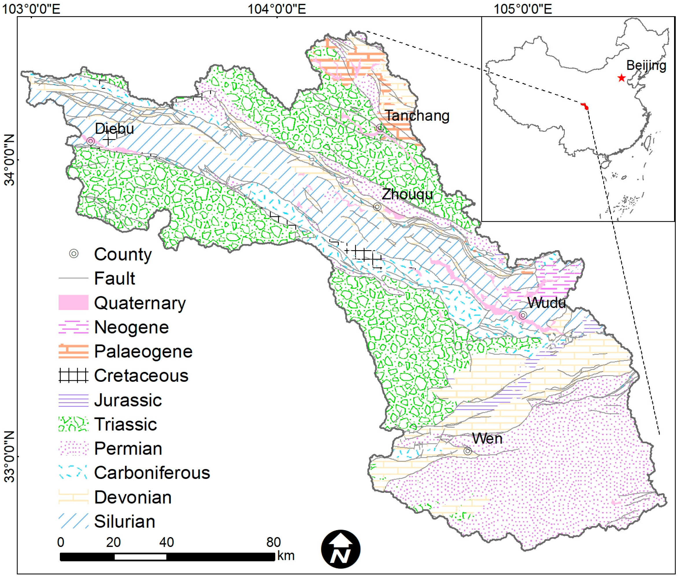
2. Study Area
3. Data and Methods
3.1. Debris Flow Inventory
3.2. Factors Influencing Debris Flows
3.2.1. Factors Related to Geomorphic Conditions
3.2.2. Factors Related to Material Conditions
3.2.3. Factors Related to Triggering Conditions
3.3. Machine Learning Analysis
3.3.1. Machine Learning Algorithms
3.3.2. Data Processing
3.3.3. Cross−Validation
3.3.4. Model Evaluation and Optimization
3.3.5. Feature Importance
4. Results
4.1. Spatial Distribution Division
4.2. Model Evaluation and Optimization
4.3. Importance of the Factors
5. Discussion
5.1. Spatial Distribution and Influencing Factors
5.2. Feature Importance Analysis
5.3. Estimation of Daily Rainfall Threshold
5.4. Uncertainties
6. Conclusions
- The main factor controlling debris flows in the study area is lithology. The medium, hard and very soft lithologies control the major distribution of debris flow catchments.
- Landslides and the factors affecting slope stability (including roads, faults and earthquakes) are the second most important factors. The factor that can be easily controlled is road construction, although controlling this may adversely affect regional economic development.
- The most important triggering factor of debris flows is the average annual frequency of daily rainfall >20 mm. We also estimated the daily rainfall thresholds of debris flows in different zones.
- The area proportion of forest and vegetation cover are also important factors controlling debris flows, which can be an important part of debris flow mitigation measures.
Author Contributions
Funding
Data Availability Statement
Acknowledgments
Conflicts of Interest
References
- Zhao, Y.; Meng, X.; Qi, T.; Qing, F.; Xiong, M.; Li, Y.; Guo, P.; Chen, G. AI-based identification of low-frequency debris flow catchments in the Bailong River basin, China. Geomorphology 2020, 359, 107125. [Google Scholar] [CrossRef]
- Jomelli, V.; Pavlova, I.; Giacona, F.; Zgheib, T.; Eckert, N. Respective influence of geomorphologic and climate conditions on debris-flow occurrence in the Northern French Alps. Landslides 2019, 16, 1871–1883. [Google Scholar] [CrossRef]
- Jakob, M.; Bovis, M.; Oden, M. The significance of channel recharge rates for estimating debris-flow magnitude and frequency. Earth Surf. Process. Landf. 2005, 30, 755–766. [Google Scholar] [CrossRef]
- Zimmermann, M.; Haeberli, W. Climatic change and debris flow activity in high-mountain areas—A case study in the Swiss Alps. Catena Suppl. 1992, 22, 59–72. [Google Scholar]
- Zimmermann, M.; Mani, P.; Romang, H. Magnitude-frequency aspects of alpine debris flows. Eclogae Geol. Helv. 1997, 90, 415–420. [Google Scholar] [CrossRef]
- Bovis, M.J.; Jakob, M. The role of debris supply conditions in predicting debris flow activity. Earth Surf. Process. Landf. 1999, 24, 1039–1054. [Google Scholar] [CrossRef]
- Glade, T. Linking debris-flow hazard assessments with geomorphology. Geomorphology 2005, 66, 189–213. [Google Scholar] [CrossRef]
- Cheng, W.; Wang, N.; Zhao, M.; Zhao, S. Relative tectonics and debris flow hazards in the Beijing mountain area from DEM-derived geomorphic indices and drainage analysis. Geomorphology 2016, 257, 134–142. [Google Scholar] [CrossRef]
- Chang, T.C.; Chao, R.J. Application of back-propagation networks in debris flow prediction. Eng. Geol. 2006, 85, 270–280. [Google Scholar] [CrossRef]
- Kovanen, D.J.; Slaymaker, O. The morphometric and stratigraphic framework for estimates of debris flow incidence in the North Cascades foothills, Washington State, USA. Geomorphology 2008, 99, 224–245. [Google Scholar] [CrossRef]
- Bertrand, M.; Liébault, F.; Piégay, H. Debris-flow susceptibility of upland catchments. Nat. Hazards 2013, 67, 497–511. [Google Scholar] [CrossRef]
- Liu, J.J.; Li, Y.; Su, P.C.; Cheng, Z.L. Magnitude–frequency relations in debris flow. Environ. Geol. 2008, 55, 1345–1354. [Google Scholar] [CrossRef]
- Johnson, P.A.; McCuen, R.H.; Hromadka, T.V. Magnitude and frequency of debris flows. J. Hydrol. 1991, 123, 69–82. [Google Scholar] [CrossRef]
- Qing, F.; Zhao, Y.; Meng, X.; Su, X.; Qi, T.; Yue, D. Application of Machine Learning to Debris Flow Susceptibility Mapping along the China–Pakistan Karakoram Highway. Remote Sens. 2020, 12, 2933. [Google Scholar] [CrossRef]
- Qi, T.; Zhao, Y.; Meng, X.; Chen, G.; Dijkstra, T. AI-Based Susceptibility Analysis of Shallow Landslides Induced by Heavy Rainfall in Tianshui, China. Remote Sens. 2021, 13, 1819. [Google Scholar] [CrossRef]
- Esper Angillieri, M.Y. Debris flow susceptibility mapping using frequency ratio and seed cells, in a portion of a mountain international route, Dry Central Andes of Argentina. Catena 2020, 189, 104504. [Google Scholar] [CrossRef]
- Imaizumi, F.; Sidle, R.C.; Kamei, R. Effects of forest harvesting on the occurrence of landslides and debris flows in steep terrain of central Japan. Earth Surf. Process. Landf. 2008, 33, 827–840. [Google Scholar] [CrossRef]
- Ghestem, M.; Veylon, G.; Bernard, A.; Vanel, Q.; Stokes, A. Influence of plant root system morphology and architectural traits on soil shear resistance. Plant Soil 2014, 377, 43–61. [Google Scholar] [CrossRef]
- Winter, M.G.; Smith, J.T.; Fotopoulou, S.; Pitilakis, K.; Mavrouli, O.; Corominas, J.; Argyroudis, S. An expert judgement approach to determining the physical vulnerability of roads to debris flow. Bull. Eng. Geol. Environ. 2014, 73, 291–305. [Google Scholar] [CrossRef]
- Guo, X.; Chen, X.; Song, G.; Zhuang, J.; Fan, J. Debris flows in the Lushan earthquake area: Formation characteristics, rainfall conditions, and evolutionary tendency. Nat. Hazards 2021, 106, 2663–2687. [Google Scholar] [CrossRef]
- Rengers, F.K.; McGuire, L.A.; Coe, J.A.; Kean, J.W.; Baum, R.L.; Staley, D.M.; Godt, J.W. The influence of vegetation on debris-flow initiation during extreme rainfall in the northern Colorado Front Range. Geology 2016, 44, 823–826. [Google Scholar] [CrossRef]
- Rogelis, M.C.; Werner, M. Regional debris flow susceptibility analysis in mountainous peri-urban areas through morphometric and land cover indicators. Nat. Hazards Earth Syst. Sci. 2014, 14, 3043–3064. [Google Scholar] [CrossRef] [Green Version]
- Lorente, A.; García-Ruiz, J.M.; Beguería, S.; Arnáez, J. Factors explaining the spatial distribution of hillslope debris flows: A case study in the Flysch Sector of the Central Spanish Pyrenees. Mt. Res. Dev. 2002, 22, 32–39. [Google Scholar] [CrossRef] [Green Version]
- Jomelli, V.; Pech, V.P.; Chochillon, C.; Brunstein, D. Geomorphic Variations of Debris Flows and Recent Climatic Change in the French Alps. Clim. Chang. 2004, 64, 77–102. [Google Scholar] [CrossRef]
- Jomelli, V.; Brunstein, D.; Grancher, D.; Pech, P. Is the response of hill slope debris flows to recent climate change univocal? A case study in the Massif des Ecrins (French Alps). Clim. Chang. 2007, 85, 119–137. [Google Scholar] [CrossRef]
- Kean, J.W.; Staley, D.M. Forecasting the Frequency and Magnitude of Postfire Debris Flows Across Southern California. Earth’s Future 2021, 9, e2020EF001735. [Google Scholar] [CrossRef]
- Pelfini, M.; Santilli, M. Frequency of debris flows and their relation with precipitation: A case study in the Central Alps, Italy. Geomorphology 2008, 101, 721–730. [Google Scholar] [CrossRef]
- Van Steijn, H. Debris-flow magnitude—frequency relationships for mountainous regions of Central and Northwest Europe. Geomorphology 1996, 15, 259–273. [Google Scholar] [CrossRef]
- Frank, F.; McArdell, B.W.; Huggel, C.; Vieli, A. The importance of entrainment and bulking on debris flow runout modeling: Examples from the Swiss Alps. Nat. Hazards Earth Syst. Sci. 2015, 15, 2569–2583. [Google Scholar] [CrossRef] [Green Version]
- Frank, F.; Huggel, C.; McArdell, B.W.; Vieli, A. Landslides and increased debris-flow activity: A systematic comparison of six catchments in Switzerland. Earth Surf. Process. Landf. 2019, 44, 699–712. [Google Scholar] [CrossRef]
- Kern, A.N.; Addison, P.; Oommen, T.; Salazar, S.E.; Coffman, R.A. Machine Learning Based Predictive Modeling of Debris Flow Probability Following Wildfire in the Intermountain Western United States. Math. Geosci. 2017, 49, 717–735. [Google Scholar] [CrossRef]
- Wieczorek, G.F.; Harp, E.L.; Mark, R.K.; Bhattacharyya, A.K. Debris flows and other landslides in San Mateo, Santa Cruz, Contra Costa, Alameda, Napa, Solano, Sonoma, Lake, and Yolo Counties, and factors influencing debris-flow distribution. In Proceedings of the Landslides, Floods, and Marine Effects of the Storm, San Francisco Bay region, CA, USA, 3–5 January 1982; U.S. Geological Survey: Reston, VA, USA, 1988; pp. 133–162. [Google Scholar]
- He, Y.P.; Chen, J.; Li, Y.; Cui, P. Debris-flow distribution and hazards along the Sichuan-Tibet and Sino-Nepal highway, Tibet, China. In Proceedings of the 3rd International Conference on Debris-Flow Hazards Mitigation: Mechanics, Prediction, and Assessment; Millpress Sciences Publishers: Davos, Switzerland, 2003; Volume 2, pp. 955–964. [Google Scholar]
- Wieczorek, G.F.; Mossa, G.S.; Morgan, B.A. Regional debris-flow distribution and preliminary risk assessment from severe storm events in the Appalachian Blue Ridge Province, USA. Landslides 2004, 1, 53–59. [Google Scholar] [CrossRef]
- Wei, F.; Jiang, Y.; Zhao, Y.; Xu, A.; Gardner, J.S. The distribution of debris flows and debris flow hazards in southeast China. In Monitoring, Simulation, Prevention and Remediation of Dense and Debris Flows III; Wessex Institute of Technology Press: Ashurst, UK, 2010; Volume 67, pp. 137–147. [Google Scholar]
- He, N.; Chen, N.S. Study on China’s Debris Flow Distribution and Occurrence Trend. Appl. Mech. Mater. 2012, 204–208, 3345–3350. [Google Scholar] [CrossRef]
- Lin, C.-W.; Liu, S.-H.; Lee, S.-Y.; Liu, C.-C. Impacts of the Chi-Chi earthquake on subsequent rainfall-induced landslides in central Taiwan. Eng. Geol. 2006, 86, 87–101. [Google Scholar] [CrossRef]
- Lin, C.W.; Shieh, C.L.; Yuan, B.D.; Shieh, Y.C.; Liu, S.H.; Lee, S.Y. Impact of Chi-Chi earthquake on the occurrence of landslides and debris flows: Example from the Chenyulan River watershed, Nantou, Taiwan. Eng. Geol. 2004, 71, 49–61. [Google Scholar] [CrossRef]
- Tang, C.; Zhu, J.; Li, W.L.; Liang, J.T. Rainfall-triggered debris flows following the Wenchuan earthquake. Bull. Eng. Geol. Environ. 2009, 68, 187–194. [Google Scholar] [CrossRef]
- Cui, P.; Chen, X.Q.; Zhu, Y.Y.; Su, F.H.; Wei, F.Q.; Han, Y.S.; Liu, H.J.; Zhuang, J.Q. The Wenchuan Earthquake (May 12, 2008), Sichuan Province, China, and resulting geohazards. Nat. Hazards 2011, 56, 19–36. [Google Scholar] [CrossRef]
- Huang, R.; Fan, X. The landslide story. Nat. Geosci. 2013, 6, 325–326. [Google Scholar] [CrossRef]
- Fan, X.; Scaringi, G.; Korup, O.; West, A.J.; Westen, C.J.; Tanyas, H.; Hovius, N.; Hales, T.C.; Jibson, R.W.; Allstadt, K.E.; et al. Earthquake-Induced Chains of Geologic Hazards: Patterns, Mechanisms, and Impacts. Rev. Geophys. 2019, 57, 421–503. [Google Scholar] [CrossRef] [Green Version]
- Hu, X.; Hu, K.; Tang, J.; You, Y.; Wu, C. Assessment of debris-flow potential dangers in the Jiuzhaigou Valley following the August 8, 2017, Jiuzhaigou earthquake, western China. Eng. Geol. 2019, 256, 57–66. [Google Scholar] [CrossRef]
- Dai, L.; Scaringi, G.; Fan, X.; Yunus, A.P.; Liu-Zeng, J.; Xu, Q.; Huang, R. Coseismic Debris Remains in the Orogen Despite a Decade of Enhanced Landsliding. Geophys. Res. Lett. 2021, 48, e2021GL095850. [Google Scholar] [CrossRef]
- Zhao, Y.; Meng, X.; Qi, T.; Li, Y.; Chen, G.; Yue, D.; Qing, F. AI-based rainfall prediction model for debris flows. Eng. Geol. 2021, 106456. [Google Scholar] [CrossRef]
- Qi, T.; Meng, X.; Qing, F.; Zhao, Y.; Shi, W.; Chen, G.; Zhang, Y.; Li, Y.; Yue, D.; Su, X.; et al. Distribution and characteristics of large landslides in a fault zone: A case study of the NE Qinghai-Tibet Plateau. Geomorphology 2021, 379, 107592. [Google Scholar] [CrossRef]
- Xiong, M.; Meng, X.; Wang, S.; Guo, P.; Li, Y.; Chen, G.; Qing, F.; Cui, Z.; Zhao, Y. Effectiveness of debris flow mitigation strategies in mountainous regions. Prog. Phys. Geogr. 2016, 40, 768–793. [Google Scholar] [CrossRef]
- Tang, C.; Rengers, N.; van Asch, T.W.J.; Yang, Y.H.; Wang, G.F. Triggering conditions and depositional characteristics of a disastrous debris flow event in Zhouqu city, Gansu Province, northwestern China. Nat. Hazards Earth Syst. Sci. 2011, 11, 2903–2912. [Google Scholar] [CrossRef] [Green Version]
- Iverson, R.M. The physics of debris flows. Rev. Geophys. 1997, 35, 245–296. [Google Scholar] [CrossRef] [Green Version]
- Wei, F.; Gao, K.; Hu, K.; Li, Y.; Gardner, J.S. Relationships between debris flows and earth surface factors in Southwest China. Environ. Geol. 2008, 55, 619–627. [Google Scholar] [CrossRef]
- Singh, P.; Thakur, J.K.; Singh, U.C. Morphometric analysis of Morar River Basin, Madhya Pradesh, India, using remote sensing and GIS techniques. Environ. Earth Sci. 2013, 68, 1967–1977. [Google Scholar] [CrossRef]
- Zhao, Y. Calculation Methods of Commonly Used Basin Geomorphological Parameters. Available online: http://0-dx-doi-org.brum.beds.ac.uk/10.13140/RG.2.2.12459.77605/3 (accessed on 20 November 2021).
- Li, Y.; Wang, H.; Chen, J.; Shang, Y. Debris Flow Susceptibility Assessment in the Wudongde Dam Area, China Based on Rock Engineering System and Fuzzy C-Means Algorithm. Water 2017, 9, 669. [Google Scholar] [CrossRef]
- Stevaux, J.C.; de Azevedo Macedo, H.; Assine, M.L.; Silva, A. Changing fluvial styles and backwater flooding along the Upper Paraguay River plains in the Brazilian Pantanal wetland. Geomorphology 2020, 350, 106906. [Google Scholar] [CrossRef]
- Wilford, D.J.; Sakals, M.E.; Innes, J.L.; Sidle, R.C.; Bergerud, W.A. Recognition of debris flow, debris flood and flood hazard through watershed morphometrics. Landslides 2004, 1, 61–66. [Google Scholar] [CrossRef] [Green Version]
- Zhou, W.; Tang, C.; Van Asch, T.W.J.; Chang, M. A rapid method to identify the potential of debris flow development induced by rainfall in the catchments of the Wenchuan earthquake area. Landslides 2016, 13, 1243–1259. [Google Scholar] [CrossRef]
- Chu, H.; Wu, W.; Wang, Q.J.; Nathan, R.; Wei, J. An ANN-based emulation modelling framework for flood inundation modelling: Application, challenges and future directions. Environ. Model. Softw. 2020, 124, 104587. [Google Scholar] [CrossRef]
- Schumm, S.A. Evolution of drainage systems and slopes in badlands at Perth Amboy, New Jersey. Bull. Geol. Soc. Am. 1956, 67, 597–646. [Google Scholar] [CrossRef]
- Schumm, S.A. The relation of drainage basin relief to sediment loss. In Proceedings of the International Union Geodesy Geophysics, 10th General Assembly (Rome); International Association of Scientific Hydrology: Rome, Italy, 1954; Volume 36, pp. 216–219. [Google Scholar]
- Melton, M.A. An Analysis of the Relations among Elements of Climate, Surface Properties, and Geomorphology; Technical Report No. 11; Columbia University, Department of Geology, Office of Naval Research: New York, NY, USA, 1957. [Google Scholar]
- Horton, R.E. Drainage-basin characteristics. EOS Trans. Am. Geophys. Union 1932, 13, 350–361. [Google Scholar] [CrossRef]
- Potter, P.E. A Quantitative Geomorphic Study of Drainage Basin Characteristics in the Clinch Mountain Area, Virginia and Tennessee. V. C. Miller. J. Geol. 1957, 65, 112–113. [Google Scholar] [CrossRef]
- Strahler, A.N. Quantitative analysis of watershed geomorphology. Eos Trans. Am. Geophys. Union 1957, 38, 913–920. [Google Scholar] [CrossRef] [Green Version]
- Strahler, A.N. Hypsometric (area-altitude) analysis of erosional topography. Bull. Geol. Soc. Am. 1952, 63, 1117–1142. [Google Scholar] [CrossRef]
- Wood, W.F.; Snell, J.B. A Quantitative System for Classifying Landforms; Technical Report EP-124; U.S. Army Quartermaster Research and Engineering Center: Natick, MA, USA, 1960. [Google Scholar]
- Church, M.; Mark, D.M. On size and scale in geomorphology. Prog. Phys. Geogr. 1980, 4, 342–390. [Google Scholar] [CrossRef]
- Wilson, M.F.J.; O’Connell, B.; Brown, C.; Guinan, J.C.; Grehan, A.J. Multiscale terrain analysis of multibeam bathymetry data for habitat mapping on the continental slope. Mar. Geod. 2007, 30, 3–35. [Google Scholar] [CrossRef] [Green Version]
- Beven, K.J.; Kirkby, M.J. A physically based, variable contributing area model of basin hydrology. Hydrol. Sci. Bull. 1979, 24, 43–69. [Google Scholar] [CrossRef] [Green Version]
- Moore, I.D.; Grayson, R.B.; Ladson, A.R. Digital terrain modelling: A review of hydrological, geomorphological, and biological applications. Hydrol. Process. 1991, 5, 3–30. [Google Scholar] [CrossRef]
- Hoek, E.; Brown, E.T. Practical estimates of rock mass strength. Int. J. Rock Mech. Min. Sci. 1997, 34, 1165–1186. [Google Scholar] [CrossRef]
- Brideau, M.-A.; Yan, M.; Stead, D. The role of tectonic damage and brittle rock fracture in the development of large rock slope failures. Geomorphology 2009, 103, 30–49. [Google Scholar] [CrossRef]
- Xie, H.; Dong, J.; Shen, Z.; Chen, L.; Lai, X.; Qiu, J.; Wei, G.; Peng, Y.; Chen, X. Intra- and inter-event characteristics and controlling factors of agricultural nonpoint source pollution under different types of rainfall-runoff events. Catena 2019, 182, 104105. [Google Scholar] [CrossRef]
- Xu, X. Chinese Population Spatial Distribution Kilometer Grid Data Set. Available online: http://www.resdc.cn/DOI (accessed on 20 November 2021).
- Lin, H.-M.; Chang, S.-K.; Wu, J.-H.; Juang, C.H. Neural network-based model for assessing failure potential of highway slopes in the Alishan, Taiwan Area: Pre- and post-earthquake investigation. Eng. Geol. 2009, 104, 280–289. [Google Scholar] [CrossRef]
- Chang, S.-K.; Lee, D.-H.; Wu, J.-H.; Juang, C.H. Rainfall-based criteria for assessing slump rate of mountainous highway slopes: A case study of slopes along Highway 18 in Alishan, Taiwan. Eng. Geol. 2011, 118, 63–74. [Google Scholar] [CrossRef]
- Guyon, I.; Weston, J.; Barnhill, S.; Vapnik, V. Gene selection for cancer classification using support vector machines. Mach. Learn. 2002, 46, 389–422. [Google Scholar] [CrossRef]
- Li, X.; Wang, Y.; Basu, S.; Kumbier, K.; Yu, B. A Debiased MDI Feature Importance Measure for Random Forests. In Proceedings of the 33rd Conference on Neural Information Processing Systems (NeurIPS 2019), Vancouver, BC, Canada, 8–14 December 2019. [Google Scholar]
- Dietrich, A.; Krautblatter, M. Evidence for enhanced debris-flow activity in the Northern Calcareous Alps since the 1980s (Plansee, Austria). Geomorphology 2017, 287, 144–158. [Google Scholar] [CrossRef]
- Liang, Z.; Wang, C.; Ma, D.; Khan, K.U.J. Exploring the potential relationship between the occurrence of debris flow and landslides. Nat. Hazards Earth Syst. Sci. 2021, 21, 1247–1262. [Google Scholar] [CrossRef]
- Iverson, R.M.; Reid, M.E.; LaHusen, R.G. Debris-flow mobilization from landslides. Annu. Rev. Earth Planet. Sci. 1997, 25, 85–138. [Google Scholar] [CrossRef]
- Li, J.; Wang, X.; Jia, H.; Liu, Y.; Zhao, Y.; Shi, C.; Zhang, F.; Wang, K. Assessing the soil moisture effects of planted vegetation on slope stability in shallow landslide-prone areas. J. Soils Sediments 2021, 21, 2551–2565. [Google Scholar] [CrossRef]
- Li, K.; Yue, D.; Guo, J.; Jiang, F.; Zeng, J.; Zou, M.; Segarra, E. Geohazards mitigation strategies simulation and evaluation based on surface runoff depth: A case study in Bailong River basin. Catena 2019, 173, 1–8. [Google Scholar] [CrossRef]
- Shen, P.; Zhang, L.M.; Chen, H.X.; Gao, L. Role of vegetation restoration in mitigating hillslope erosion and debris flows. Eng. Geol. 2017, 216, 122–133. [Google Scholar] [CrossRef]
- Balzano, B.; Tarantino, A.; Ridley, A. Preliminary analysis on the impacts of the rhizosphere on occurrence of rainfall-induced shallow landslides. Landslides 2019, 16, 1885–1901. [Google Scholar] [CrossRef] [Green Version]
- Shen, P.; Zhang, L.M.; Fan, R.L.; Zhu, H.; Zhang, S. Declining geohazard activity with vegetation recovery during first ten years after the 2008 Wenchuan earthquake. Geomorphology 2020, 352, 106989. [Google Scholar] [CrossRef]
- Wang, S.; Meng, X.; Chen, G.; Guo, P.; Xiong, M.; Zeng, R. Effects of vegetation on debris flow mitigation: A case study from Gansu province, China. Geomorphology 2017, 282, 64–73. [Google Scholar] [CrossRef]
- Zhao, Y. DF_distribution.zip. Available online: http://0-dx-doi-org.brum.beds.ac.uk/10.13140/RG.2.2.11129.19048 (accessed on 20 November 2021).


| Stratigraphic Age | Major Lithology | GSI | Relative Strength |
|---|---|---|---|
| Quaternary loose material | Pebbles, gravel, silty clay | 0–10 | very soft |
| Neogene stratified clastic rocks | Conglomerate, shale, sandstone | ||
| Paleogene stratified clastic rocks | Conglomerate | ||
| Cretaceous stratified clastic rocks | Conglomerate, sandstone, mudstone | 10–20 | soft |
| Jurassic stratified clastic rocks | Sandstone, mudstone, conglomerate, shale | 30–40 | medium |
| Silurian metamorphic rocks | Sandstone, limestone, phyllite, slate | ||
| Devonian carbonate rocks | Slate, phyllite, limestone | ||
| Permian layered metamorphic rocks | Sandstone, sandy slate, tuff, phyllite | ||
| Carboniferous carbonate rocks | Limestone | 60–70 | hard |
| Devonian carbonate rocks | Limestone, shale, slate, sandstone | ||
| Triassic and Permian layered carbonate | Limestone, sandstone, shale | ||
| Triassic and Permian intrusive rocks | Granite, diorite, granite gneiss, basalt, diabase | 80–90 | very hard |
| No. | Parameter | Abbr. | Formula | Unit |
|---|---|---|---|---|
| 1 | Basin area | A | GIS analysis | km2 |
| 2 | Main channel length | Lmc | GIS analysis | km |
| 3 | Curvature of the main stream | Cms | Cms = Lmc/Ls | / |
| 4 | Average slope | Sa | Average value | ° |
| 5 | Area proportion of slopes > 30° | S30 | Area of slopes > 30°/A | % |
| 6 | Area proportion of slopes > 35° | S35 | Area of slopes > 35°/A | % |
| 7 | Area proportion of slopes > 40° | S40 | Area of slopes > 40°/A | % |
| 8 | Area proportion of slopes between 30° and 40° | S30–40 | Area of slopes 30–40°/A | % |
| 9 | Average aspect | Aa | Average value | ° |
| 10 | Basin relief | H | H = Hmax − Hmin | km |
| 11 | Relief ratio | Rr | Rr = H/L | / |
| 12 | Relative relief ratio | Rrr | Rrr = H*100/p | / |
| 13 | Drainage density | Dd | Dd = Lt/A | / |
| 14 | Circularity ration | Cr | Cr = 4πA/P2 | / |
| 15 | Form factor | Ff | Ff = A/L2 | km |
| 16 | Elongation ratio | Er | / | |
| 17 | Hypsometric Integral | HI | HI = (Hmean − Hmin)/(Hmax − Hmin) | / |
| 18 | Melton ratio | Mr | / | |
| 19 | Plane curvature | Cpl | GIS analysis | / |
| 20 | Profile curvature | Cpr | GIS analysis | / |
| 21 | Ruggedness number | Rn | Rn = H*Dd | / |
| 22 | Terrain Ruggedness Index | TRI | GDAL analysis | / |
| 23 | Topographic Position Index | TPI | GDAL analysis | / |
| 24 | Topographic Wetness Index | TWI | TWI = ln(As/tan(S)) | / |
| 25 | Stream Power Index | SPI | SPI = ln(As*tan(S)) | / |
| 26 | Fitness ratio | Rf | Rf = Lmc/p | / |
| 27 | Area proportion of very hard lithology | Lvh | Area of very hard lithology/A | / |
| 28 | Area proportion of hard lithology | Lh | Area of hard lithology/A | / |
| 29 | Area proportion of moderate lithology | Lm | Area of moderate lithology/A | / |
| 30 | Area proportion of soft lithology | Ls | Area of soft lithology/A | / |
| 31 | Area proportion of very soft lithology | Lvs | Area of very soft lithology/A | / |
| 32 | Fault density | Fd | Linear density | / |
| 33 | Area proportion of unused land | Lun | Area of unused land/A | / |
| 34 | Area proportion of forest land | Lfo | Area of forest land/A | / |
| 35 | Area proportion of grass land | Lgr | Area of grass land/A | / |
| 36 | Area proportion of cultivated land | Lcu | Area of cultivated land/A | / |
| 37 | Area proportion of residential land | Lre | Area of residential land/A | / |
| 38 | Area proportion of industrial land | Lin | Area of industrial land/A | / |
| 39 | Normalized Difference Vegetation Index | NDVI | Average value | / |
| 40 | Soil depth | Sde | Average value | cm |
| 41 | Soil clay fraction | Scf | Average value | % |
| 42 | Soil bulk density | Sbd | Average value | kg/dm3 |
| 43 | Landslide density | Ld | Point density | / |
| 44 | Peak ground acceleration | PGA | Average value | / |
| 45 | Population | Pop | Average value | / |
| 46 | Gross domestic product | GDP | Average value | / |
| 47 | Road density | Rd | Linear density | / |
| 48 | Average annual frequency of rainfall > 15 mm/d | F15 | GIS analysis | times/yr |
| 49 | Average annual frequency of rainfall > 20 mm/d | F20 | GIS analysis | times/yr |
| 50 | Average annual frequency of rainfall > 30 mm/d | F30 | GIS analysis | times/yr |
| 51 | Average annual frequency of rainfall > 40 mm/d | F40 | GIS analysis | times/yr |
| 52 | Average annual frequency of rainfall > 50 mm/d | F50 | GIS analysis | times/yr |
| MLA | Optimal Parameter | Acc | Std |
|---|---|---|---|
| ETS | n_estimators = 200; max_depth = 22; criterion = entropy | 0.952 | 0.0166 |
| XGB | n_estimators = 50; learning_rate = 0.25; max_depth = 6 | 0.948 | 0.0153 |
| GB | n_estimators = 50; learning_rate = 0.25; criterion = friedman_mse; max_depth = 6 | 0.947 | 0.0173 |
| RF | n_estimators = 500; criterion = gini; oob_score = True; max_depth = 14 | 0.936 | 0.0169 |
| Acc | Std | Factors | Number | |
|---|---|---|---|---|
| Before RFECV | 0.952 | 0.0166 | A, Cms, Sa, S30–40, Aa, H, Dd, Cr, Ff, HI, Mr, Cpl, Cpr, TPI, TWI, Rf, Lvs, Ls, Lm, Lh, Lvh, Fd, Lun, Lfo, Lgr, Lcu, Lre, Lin, NDVI, Sde, Scf, Sbd, Ld, PGA, Pop, GDP, Rd, F15, F20, F50 | 40 |
| After RFECV | 0.956 | 0.0149 | Sa, Mr, Cpl, Cpr, Lvs, Lm, Lh, Fd, Lfo, Lgr, Lcu, NDVI, Sbd, Ld, PGA, Rd, F15, F20 | 18 |
| Zone | Debris Flow Frequency | >15 mm | >20 mm | >30 mm | >40 mm | >50 mm |
|---|---|---|---|---|---|---|
| High | >2 | 5–9.5 | 1–7 | 1–2 | <0.5 | <0.25 |
| Moderate | 0.5–2 | 5–8 | 2–5 | 1–3 | 0.3–1 | <0.25 |
| Low | <0.5 | 5–7 | 1–3 | 0.5–1.5 | <0.5 | <0.25 |
Publisher’s Note: MDPI stays neutral with regard to jurisdictional claims in published maps and institutional affiliations. |
© 2021 by the authors. Licensee MDPI, Basel, Switzerland. This article is an open access article distributed under the terms and conditions of the Creative Commons Attribution (CC BY) license (https://creativecommons.org/licenses/by/4.0/).
Share and Cite
Zhao, Y.; Meng, X.; Qi, T.; Chen, G.; Li, Y.; Yue, D.; Qing, F. Modeling the Spatial Distribution of Debris Flows and Analysis of the Controlling Factors: A Machine Learning Approach. Remote Sens. 2021, 13, 4813. https://0-doi-org.brum.beds.ac.uk/10.3390/rs13234813
Zhao Y, Meng X, Qi T, Chen G, Li Y, Yue D, Qing F. Modeling the Spatial Distribution of Debris Flows and Analysis of the Controlling Factors: A Machine Learning Approach. Remote Sensing. 2021; 13(23):4813. https://0-doi-org.brum.beds.ac.uk/10.3390/rs13234813
Chicago/Turabian StyleZhao, Yan, Xingmin Meng, Tianjun Qi, Guan Chen, Yajun Li, Dongxia Yue, and Feng Qing. 2021. "Modeling the Spatial Distribution of Debris Flows and Analysis of the Controlling Factors: A Machine Learning Approach" Remote Sensing 13, no. 23: 4813. https://0-doi-org.brum.beds.ac.uk/10.3390/rs13234813