
Evaluation of the Performance of Time-Series Sentinel-1 Data for Discriminating Rock Units


College of Geo-Exploration Science and Technology, Jilin University, Changchun 130026, China
*
Author to whom correspondence should be addressed.
Remote Sens. 2021, 13(23), 4824; https://0-doi-org.brum.beds.ac.uk/10.3390/rs13234824
Submission received: 13 October 2021
/
Revised: 25 November 2021
/
Accepted: 26 November 2021
/
Published: 27 November 2021
(This article belongs to the Special Issue Surface Mineral Allocation and Lithological Mapping Based on Remote Sensing)
Abstract
:The potential use of time-series Sentinel-1 synthetic aperture radar (SAR) data for rock unit discrimination has never been explored in previous studies. Here, we employed time-series Sentinel-1 data to discriminate Dananhu formation, Xinjiang group, Granite, Wusu group, Xishanyao formation, and Diorite in Xinjiang, China. Firstly, the temporal variation of the backscatter metrics (backscatter coefficient and coherence) from April to October derived from Sentinel-1, was analyzed. Then, the significant differences of the time-series SAR metrics among different rock units were checked using the Kruskal–Wallis rank sum test and Tukey’s honest significant difference test. Finally, random forest models were used to discriminate rock units. As for the input features, there were four groups: (1) time-series backscatter metrics, (2) single-date backscatter metrics, (3) time-series backscatter metrics at VV, and (4) VH channel. In each feature group, there were three sub-groups: backscatter coefficient, coherence, and combined use of backscatter coefficient and coherence. Our results showed that time-series Sentinel-1 data could improve the discrimination accuracy by roughly 9% (from 55.4% to 64.4%), compared to single-date Sentinel-1 data. Both VV and VH polarization provided comparable results. Coherence complements the backscatter coefficient when discriminating rock units. Among the six rock units, the Granite and Xinjiang group can be better differentiated than the other four rock units. Though the result still leaves space for improvement, this study further demonstrates the great potential of time-series Sentinel-1 data for rock unit discrimination.

1. Introduction
Accurate identification of lithology is important for mineral and oil exploration [1,2]. However, conventional field-based lithology investigation, especially in large areas or areas with substantial amounts of cover, is often time-consuming and expensive. Recent advances in remote sensing techniques provide excellent tools to conduct geological studies, such as mapping lithological units, cost- and time-efficiently [3,4].
Previous studies indicated that diagnostic spectral signatures could be affected by various physical and chemical properties such as the rock-forming compositions [5,6], structure [7], particle size [8,9], and molecular vibration [10,11,12]. These studies build a profound basis for subsequent research on distinguishing rock units using airborne/satellite remote sensing data. Over the past few decades, various optical satellite remote sensing data ranging from multispectral to hyperspectral and low resolution to high resolution has been utilized in lithology-related studies [13,14,15,16,17]. However, lithology discrimination often suffers from low accuracy due to the overlap of the diagnostic spectral features or the spectral variability of rocks [18,19].
To obtain more lithological information, multiple data and advanced methods have been considered. Methods including principal component analysis [20,21], independent component analysis [16], support vector machine [22,23], random forest (RF) [24], and neural network [25] have deployed fruitful results in lithology mapping. Data integration has also been suggested for improving classification accuracy. Except for multi-source spectral data [26], texture data [21], topographic data [27,28], and synthetic aperture radar (SAR) [29,30,31,32], can also offer valuable data for lithological mapping when combined with spectral imagery. However, spectral information mostly plays the dominant role, and other data usually serve as ancillary information [2,33].
Contemporary with optical imagery being widely used in geological studies, the potential of radar imagery was gradually discovered. In contrast to optical images, radar has some well-known advantages, such as the ability to observe independently from the sun illumination and penetrate the cloud cover. Dellwig and Moore [34] firstl evaluated the simultaneously produced co-/cross-polarized images obtained from NASA (National Aeronautics and Space Administration) program and indicated that the topography, surface roughness, rock types were related to the contrasts in the return value. Mccauley [35] discussed the polarization anomalies that an obvious lower cross-polarized returns than that from co-polarized returns of certain volcanic rocks. The author concluded the anomalies were mainly produced by the specular non-depolarized reflection from rock surfaces. The rich textual information provided by SAR imagery also showed promising performance on discriminating lithological units [36]. Lu et al. [37] also mentioned the usefulness of texture information derived from Sentinel-1 in lithology discrimination. The radar scattering process can be decomposed into single, double, and cross scattering, and the decomposed information can contribute to improving rock classification [38,39]. However, most of the existing decomposition models are not suitable for the dual-polarized SAR data. Wang et al. [40] compared two frequencies (L-band and C-band) in polarimetric SAR images for mapping iron-mineralized laterites, and the L-band provided superior results in comparison to C-band. Dual-frequency polarimetric SAR was used together with a deep learning method to successfully classify lithology [41]. Although the advantages of SAR data have been around for a long time for its imaging capability in moist and vegetated regions for geological survey [42], later research has proven that vegetation and topography can still limit the reliability of SAR in geological interpretation [43]. The utility of SAR complex coherence images generated from two SAR images acquired at different dates can enhance the differences between lithologies [44]. In general, most of these studies only considered the performance of mono-temporal (single-date) SAR data. To the best of our knowledge, there is no research utilizing time-series SAR data to differentiate rock units.
Remote sensing time-series data has been widely used in agriculture [45,46], forestry [47,48], deformation [49,50], and other land surface analysis such as infrastructure monitoring [51]. Time-series SAR data was usually employed due to the sensitivity to structural change [52], surface roughness [53,54], and soil moisture [55]. Normally, properties such as surface roughness and moisture content of rocks vary under different environments, and different rocks may lead to different responses to the various environmental changes. In this context, this paper involves time-series Sentinel-1 SAR images acquired over a semi-arid area to discriminate rock units using the RF algorithm. Their performance is evaluated by the kappa coefficient, confusion matrix, and overall accuracy.
2. Study Area and Data
2.1. Study Area and Field Survey
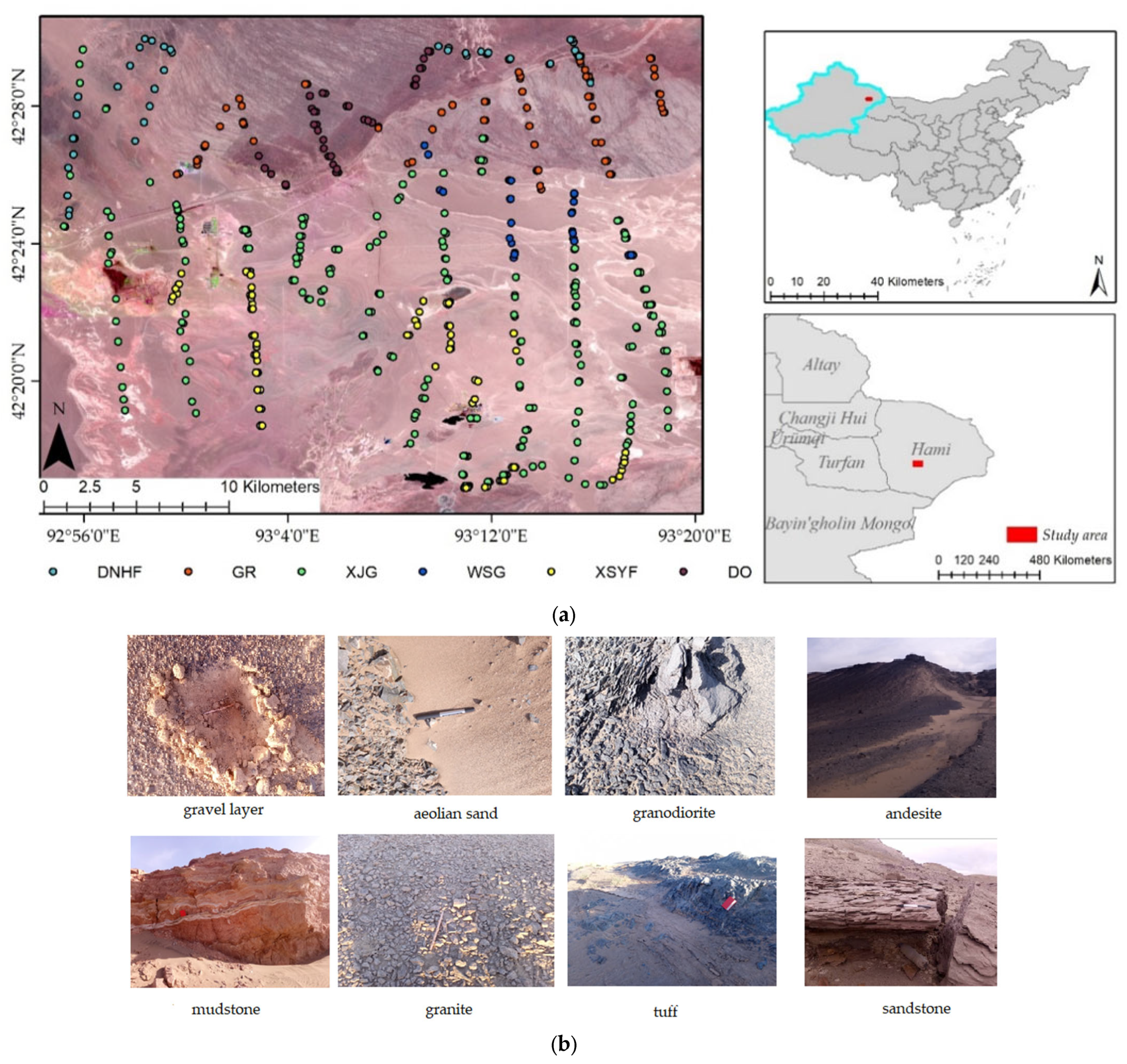
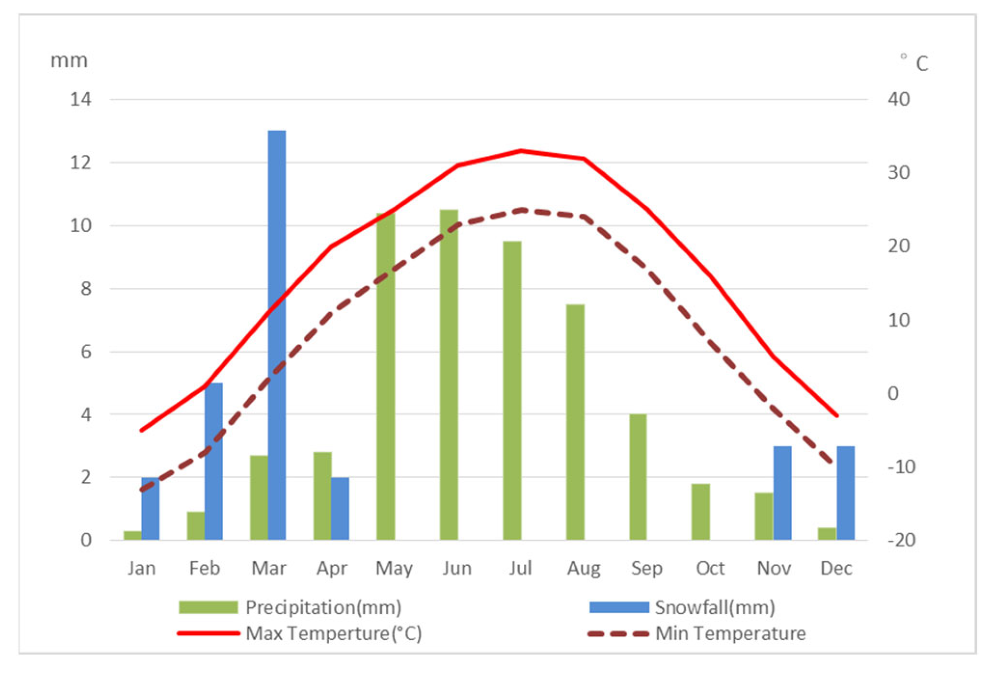
The study area (Figure 1) is within Hami, Xinjiang Province, China. The study area is situated in a continental temperate arid climate zone with low rainfall and strong wind. The dry climate prevents the development of soil and vegetation. The historical monthly averaged precipitation, snowfall, and temperature (Figure 2) were also queried to facilitate interpretation of the following results. It should be noted that temperature varies widely from day and night.
The field survey was conducted from 23 May 2020 to 4 June 2020, collecting 451 samples (Figure 1). Samples were randomly collected in accessible places. The local weathering effect, tectonic activity [56], and human activities (quarry and transportation) lead to plentiful rock exposure. The samples can generally be divided into six categories according to major components or the typical lithology: Dananhu formation, granite, Xinjiang group, Wusu group, Xishanyao formation, and diorite. Abbreviations and detailed information are listed in Table 1 [57]. All samples were collected in an open area with sparse vegetation cover.
2.2. Satellite Data
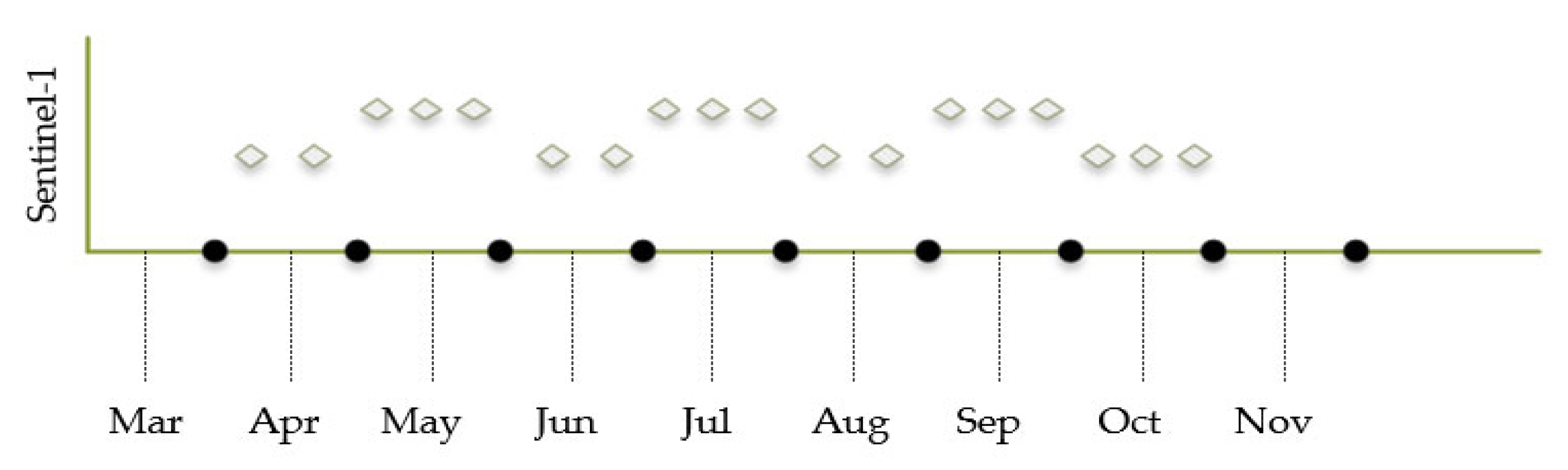
The satellite SAR data used in this study was acquired from the C-band Sentinel-1 mission, which consists of Sentinel-1A and Sentinel-1B constellations. The incidence angle of Sentinel-1 varies from 30 to 40 degrees. Only Sentinel-1A collects data over the study area with a revisit time of 12 days. To avoid the snow effect, all Sentinel-1A data from April to October in 2020 were used (Figure 3). In total, 18 GRD (ground range detected) images and 18 SLC (single-look complex) products in interferometric wide swath mode were involved. SLC products contain both amplitude and phase information in complex form. GRD products consist of focused SAR data that has been detected. All SAR scenes were dual-polarized (VV and VH).
3. Methodology
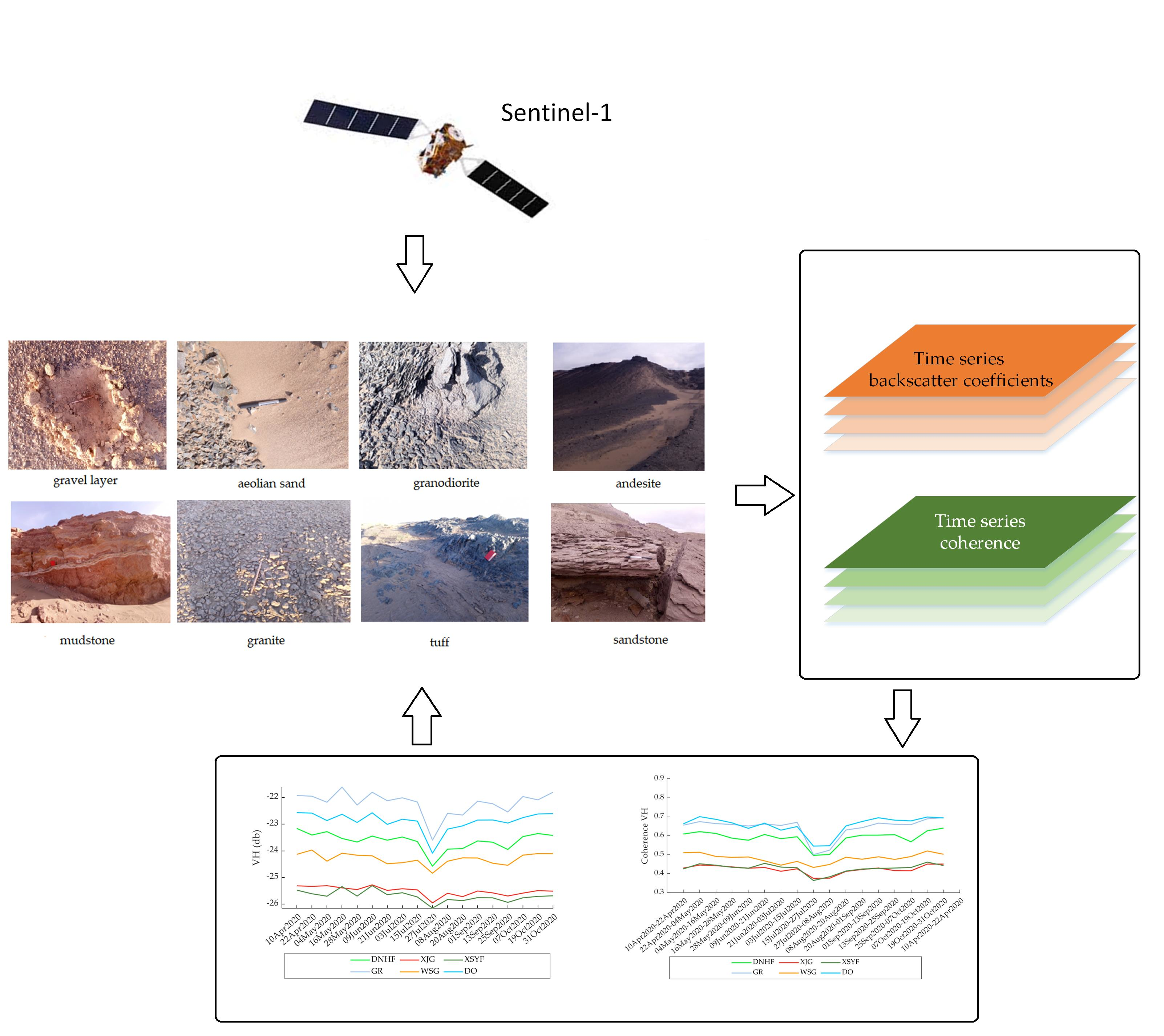
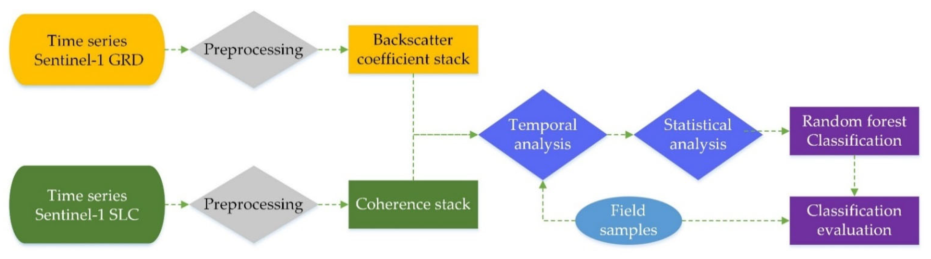
Figure 4 illustrate the general workflow adopted in this study to evaluate the performance of time series Sentinel-1 products in discriminating rock units. The workflow mainly consists of four parts: (1) the preprocessing of Sentinel-1 GRD and SLC products; (2) the temporal analysis of the SAR-derived parameters (backscatter coefficient and the coherence); (3) the statistical analysis of the SAR-derived parameters; (4) the evaluation of the rock unit discrimination using RF algorithm.
3.1. The Preprocessing of Sentinel-1 GRD and SLC Products
All of the preprocessing steps were performed using the Sentinel’s Application Platform toolbox (version 8.0) offered by the European Space Agency. In the case of Sentinel-1 GRD data, as described in [58], the orbit file correction was first applied. Then, the images were calibrated radiometrically into sigma naught, and the true SAR backscatter was related to the pixel value. The images were then subset, and the refined Lee filter was used to remove the speckle noise. At last, the images were terrain corrected with a high-resolution digital elevation model (DEM) and converted to a log scale in decibels (db).
As for Sentinel-1 SLC data, an interferometric SAR analysis was required to achieve the coherence values. The coherence value ranges from 0 (incoherent) to 1 (coherent), and is sensitive to the changes in phase and amplitude. Moreover, coherence loss can be caused by systematic spatial and temporal de-correlation and surface change [59]. Thus, the repeat pass SLC products were selected to minimize the systematic spatial error. The SLC images were first split into sub-swaths (IW1, IW2, and IW3) and the sub-swath (IW2) where the study area located was selected. Similarly, the orbit was updated with a precise orbit file. Due to the coherence yields, the normalized complex correlation between two SAR images (master and slave) acquired at two acquisition dates, and a coregistration between every two consecutive dates (every 12 days), was applied to minimize the systematic temporal induced de-correlation before coherence estimation. Then, a total of 17 coherence images were obtained for VV coherence and VH coherence individually. The demarcation zones between bursts were then removed, and all the coherence images were geocoded with the same high-resolution DEM as the process of GRD products.
After the preprocessing, the corresponding SAR parameters (coherence and backscatter coefficient) of the field samples were extracted from Sentinel-1 SLC and GRD products for the following analysis.
3.2. Temporal Analysis of the SAR-Derived Parameters
Given the limited knowledge of the spatiotemporal dynamics of rock units in a semi-arid place from a remote sensing perspective, a temporal analysis of the polarimetric parameters of each rock unit was conducted. The average values of each polarimetric parameter, (coherence and backscatter coefficient) obtained from all samples associated with each rock unit throughout the whole Sentinel-1 acquisition period (Figure 3) for both polarizations, were computed. Then, the temporal variations of the SAR-derived parameters among different rock units were compared.
3.3. Statistical Analysis of the SAR-Derived Parameters
To better understand the performance of the time-series Sentinel-1 data on discriminating rock units, the behavior of the time-series backscatter coefficient and the polarimetric coherence of different rock units derived from SLC and GRD data were analyzed via MATLAB 2020a, respectively. For each sample, the mean value of each polarimetric parameter during the period from April to October was first calculated. Hereafter, the Kruskal–Wallis rank sum test and Tukey’s honest significant difference (HSD) test were carried out. The Kruskal–Wallis rank sum test [60] is a nonparametric test that does not require a normal distribution and equal size of the data. It compares the sample means of different rock units to find if they are from the same distribution. To help interpret this, boxplots of different polarimetric parameters were plotted. Meanwhile, a post hoc Turkey’s HSD test was carried out to compute the multiple comparisons to find a significant difference among all possible pairs of means.
3.4. Evaluation of the Rock Unit Discrimination Using RF Algorithm
RF algorithm was employed for discriminating different rock units using the scikit-learn package in Python. In recent years, RF has provided a popular classifier for geologists [22,24,42]. The RF algorithm is a supervised machine learning algorithm that establishes results based on the prediction of multiple decision trees, and the class with the majority vote becomes the final prediction [61]. Bootstrap aggregation (bagging) developed by Breiman aims at reducing the variance of the prediction model. Each time, random and smaller samples (around two-thirds) originating from the training dataset were used to train the model with the left (around 1/3) out of bag samples evaluating the model error, and the outputs, were aggregated into the final result. As the the number of decision trees increase, the more reliable estimation results can be achieved; however, the computation time becomes longer at the same time as a kind of penalty. After the initial test (compute the out of bag error when the number of trees varies from 100 to 500), the number of trees was set as 200 in this study, considering both the prediction accuracy and the computation time. The maximum features and the maximum depth parameters were kept at default settings.
In this study, the input features were grouped into three groups: the time-series backscatter coefficients, the time-series coherence values, and both of these two time-series data sets. A total of 30% of the 451 field samples were randomly selected as the test dataset, and the remaining 70% of the samples were used as the training dataset. For the accuracy assessment of the RF classification results, the overall accuracy (OA), precision (user’s accuracy), recall (producer’s accuracy), kappa coefficient, F1-score, and the confusion matrix, were calculated.
4. Results
4.1. Temporal Variation of Coherence and Backscatter Coefficients among Different Rock Units
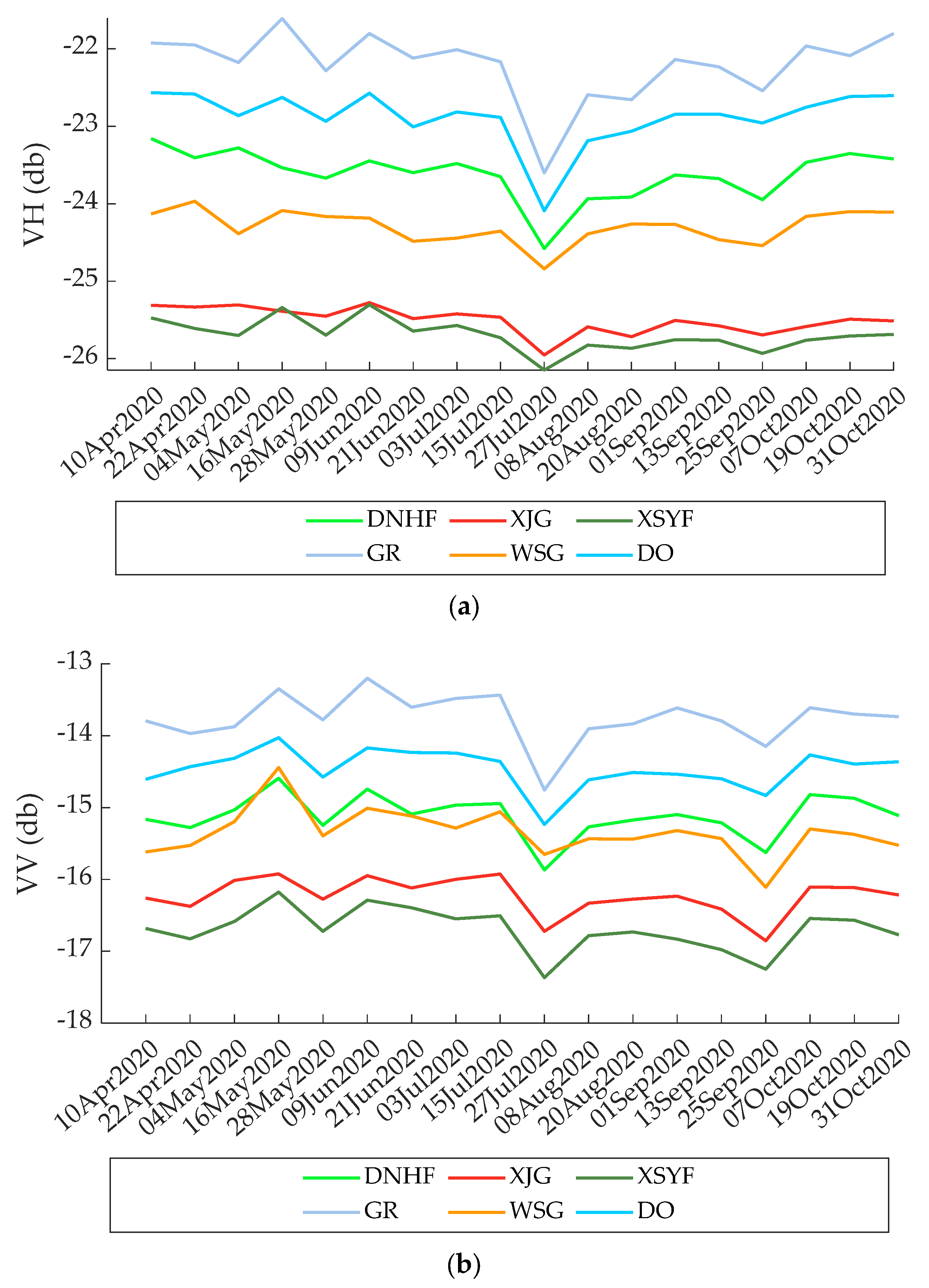
To explore how the scattering characteristics change with time, replicated measurements of the corresponding Sentinel-1 parameters for the field samples were derived from April to October. Figure 5a demonstrate the variation of the mean backscatter value in VH. There is a similar variation trend for almost all rock units (Figure 5a) in VH. From April to the start of July, the backscatter coefficient VH changed on a small scale. Hereafter, from the start of July to the end of July, there was a decrease. On 27 July 2020, all the rock units reached their bottom values at the VH channel. Then, an increase happened in early August, and the backscatter value in VH kept increasing or was stable until the end of October. Moreover, for WSG, XJG, and XSYF, the variation was not dramatic compared to other rock units. In general, the temporal variation of the mean backscatter value in VH among all rock units was separated from each other, which meant the time-series backscatter value in VH might be a good discriminator. However, the time-series backscatter value of WSG and DNHF in VV, from April to August, were intertwined several times (Figure 5b). Concerning the temporal variation of the backscatter value in VV (Figure 5b), the variation trend was a little bit different from that of VH as there was another obvious low point on 25 September among all rock units.
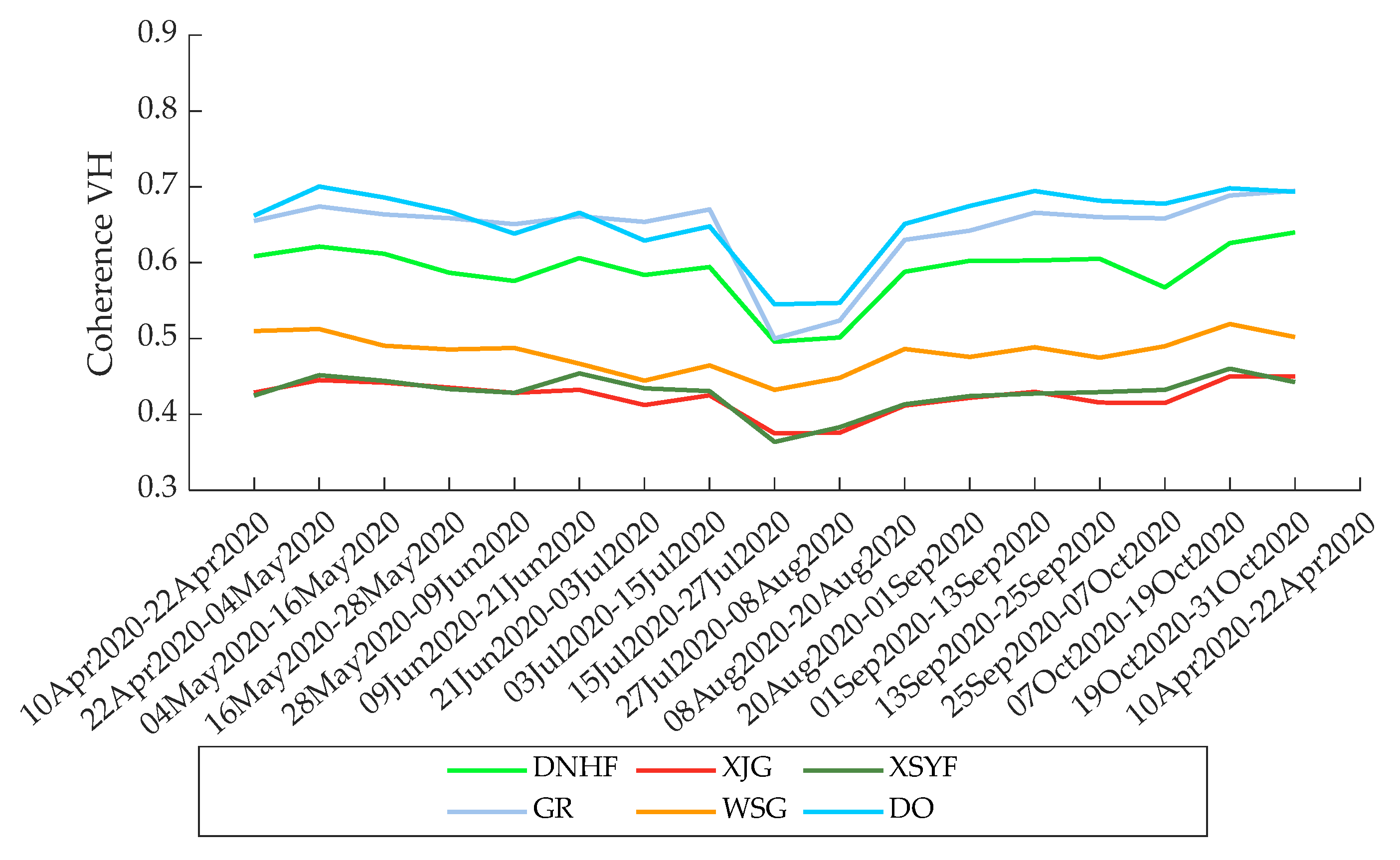
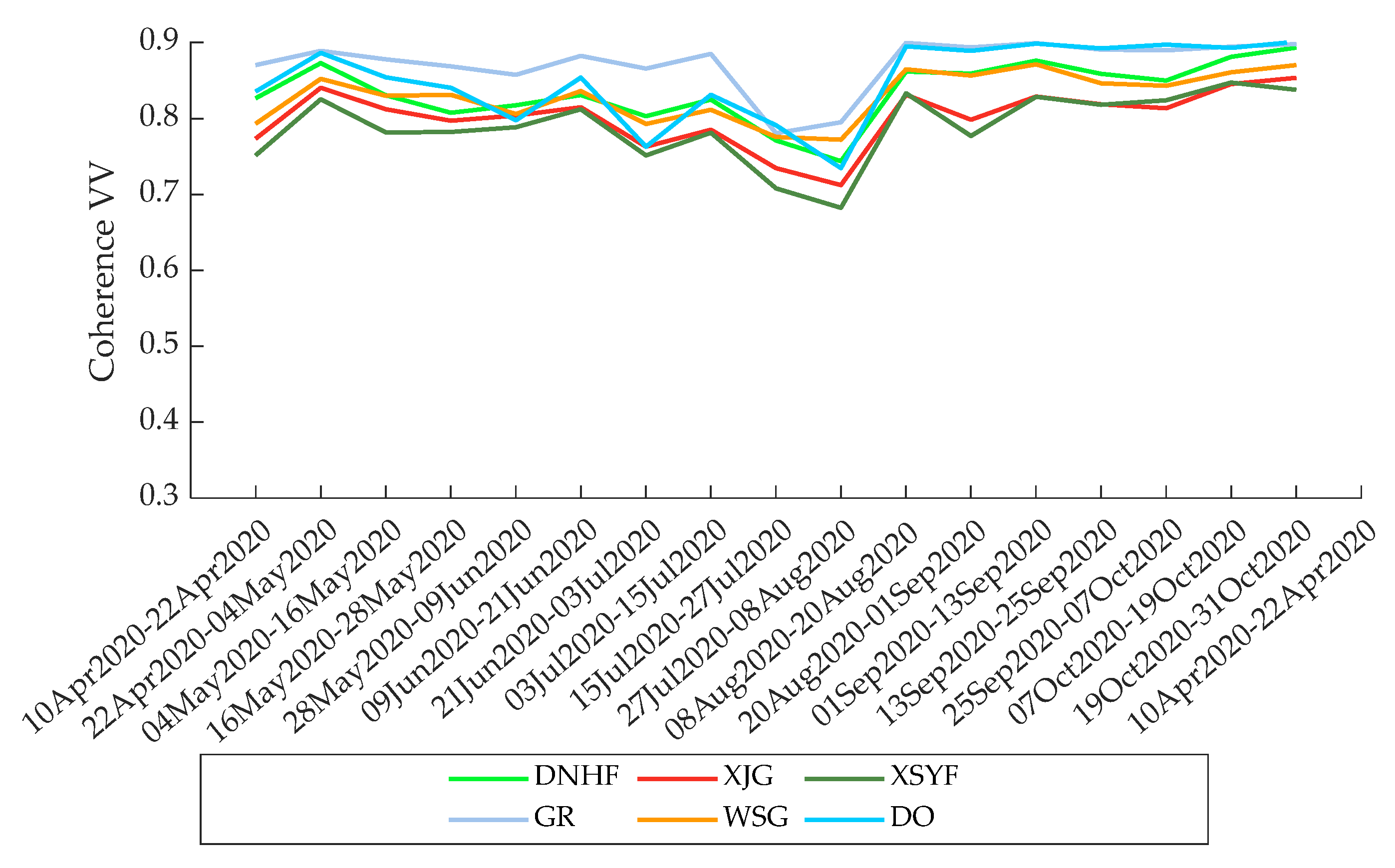
Figure 6 display the time-series VH coherence values of different rock units. It can be noticed that except for the period between 15 July and 8 August, when all VH coherence had large fluctuation, the VH coherence among all rock units had smooth variations at other times. GR and DO had higher VH coherence values than other units throughout the study period. XSYF and XJG showed the lowest VH coherence. Moreover, the VH coherence of XJG and XSYF almost overlapped. By looking at the variation of VV coherence (Figure 7), we can note that compared to the VH coherence, all rock units presented a higher VV coherence. According to Figure 7, before 27 July, the VV coherence of all rock units intertwined with other units except for GR. While after 27 July, the variation of most rock units became stable but still difficult to differentiate. Another interesting thing is that, compared to the backscatter coefficient, the coherence of both VV and VH reduced the separability among all rock units, especially the coherence of VV.
4.2. Statistical Analysis of Time-Series SAR Derived Parameters for Discriminating Rock Units
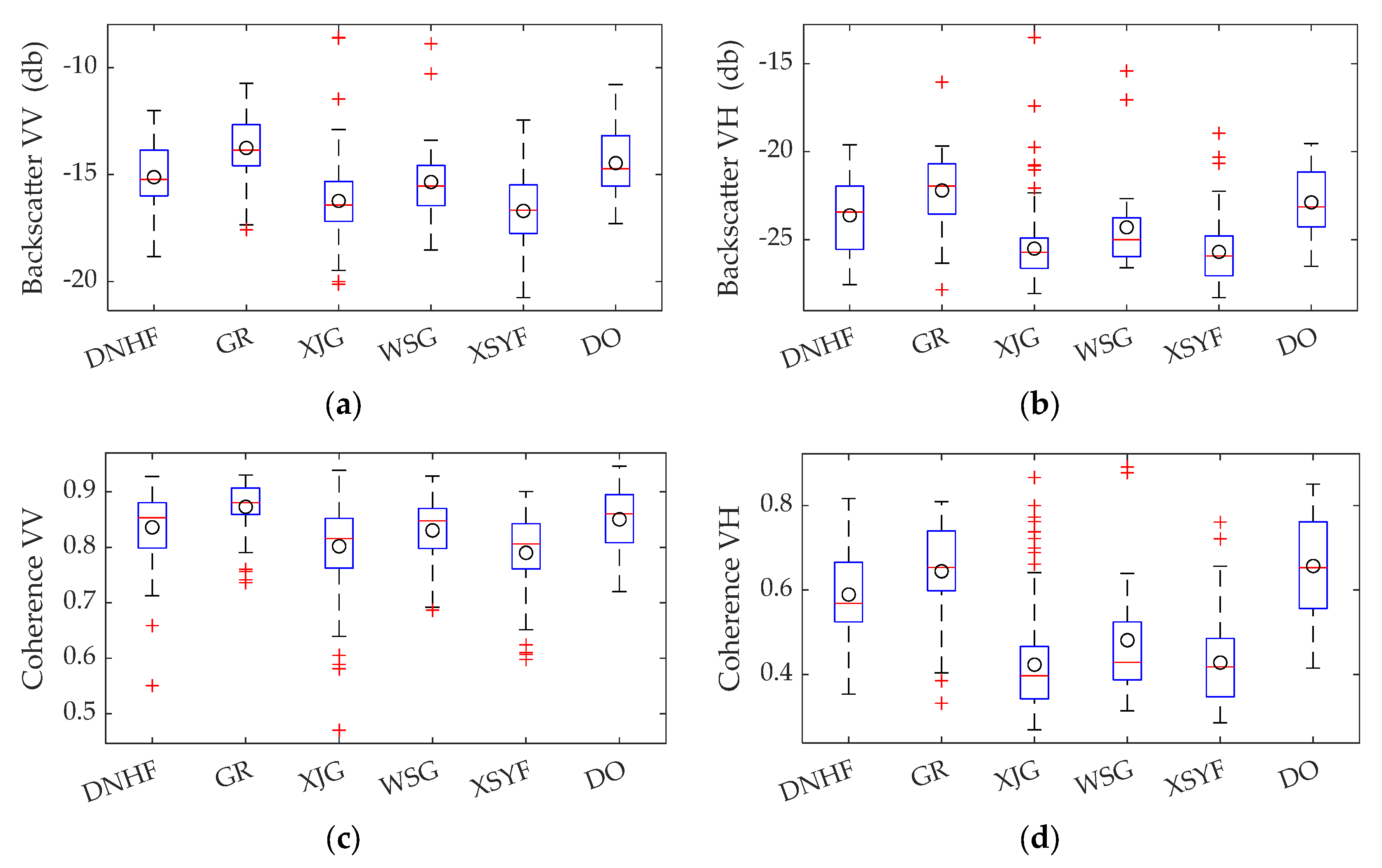
From the statistical boxplots (Figure 8), the variation of the time-series scattering characteristics among different rock units is demonstrated. According to the result of the Kruskal–Wallis rank sum test (Table 2), the mean values of all four time-series metrics derived from Sentinel-1 have significant differences among different rock units at a 99% confidence level. For each rock unit, due to the various properties, the backscatter coefficient and coherence at both channels varied over a wide range and thus lead to overlap between different units (Figure 8). For instance, the backscatter coefficients derived from XJG and XSYF had a large overlap.
As seen from Figure 8a,b, in general, the backscatter coefficient at the VV channel has a higher mean value than that of VH. GR has the highest mean backscatter value at both VV (around −13.7 db) and VH (−22.2 db) channels, followed by DO with −14.5 db in VV and −22.9 db in VH. XJG and XSYF have noticeable lower mean VV backscatter values (lower than −16 db) and mean VH backscatter values (lower than −25 db) than other rock units. DHNF (−15.1 db and –23.6 db, respectively) have a relatively higher backscatter value than that of WSG (around −15.3 db and –24.3 db, respectively).
Figure 8c,d show the variation of coherence in VV and VH. We can see that VV has a higher mean coherence than that of VH for all rock units. GR and DO have substantially high mean VV coherence (higher than 0.85). XSYF showed the lowest VV coherence locates around 0.79. In the case of the mean coherence at the VH channel, XJG, WSG, and XSYF have very low values (around 0.45). DO has the highest mean coherence in VH (0.66), followed by GR (0.64). Moreover, the variation of the mean coherence of VH among different rock units is larger than that of mean VV coherence.
Though the Kruskal–Wallis rank sum test the significant difference among different rock units was illustrated, the result of Tukey’s HSD test further showed that the significant difference only exists between some units with specific Sentinel-1 parameters (Table 3). For instance, GR was significantly different from all other classes except for DO. Only VH coherence is useful to distinguish DNHF from WSG. Overall, most of the pairwise classes can be distinguished, except for DHNF-DO, GR-DO, and XJG-XSYF.
4.3. Evaluation of the Performance of Sentinel-1 Data for Discrimination Rock Units
After the statistical analysis and the temporal analysis, RF algorithm was applied using features (coherence and backscatter coefficient) derived from Sentinel-1 throughout the period from April to October. Firstly, the time-series backscatter coefficient and coherence from both VV and VH polarizations were used as individual input features, and then these two types of features were integrated as whole input features for the RF algorithm. The results of these three cases are shown in Table 4. It is easy to see that the combined use of backscatter coefficient and coherence resulted in the highest OA (64.4%) and kappa coefficient (0.390). Both the precision and the recall obtained by the combined use of features reached almost the highest level except for the XSYF. Rock units with better F1-scores were GR and XJG (0.69 and 0.78, respectively). Units with worse results were DNHF, WSG, and XSYF. The OA and kappa coefficient from the result using the time-series backscatter coefficient were higher than that of time-series coherence. At the unit level, for most rock units, the combination of backscatter coefficient and coherence balanced the performance of these two types of features (e.g., the precision of DNHF, from 26% and 47% to 34%). A complementary effect can also be seen for some rock units. For instance, the precision of GR (an increase from 63% and 58% to 69%). Here, only the confusion matrix using the combined features (Table 5) was demonstrated and discussed. Most of WSG, XSYF, and DNHF were misclassified into XJG. Meanwhile, there was confusion between GD and GR, DNHF and GR.
To further investigate the usefulness of time-series Sentinel-1 derived features for rock unit discrimination, RF was also tested on single-date Sentinel-1 derived features. We chose the satellite images which were acquired synchronously as the fieldwork. The backscatter coefficient was derived from Sentinel-1 acquired on 28 May, and the coherence was calculated between 28 May and 16 May. It can be observed (Table 4 and Table 6) that when only single-date derived SAR features are used, compared to the time-series features, the OA decreased from 63.3%, 61.8%, and 64.4% to 50.0%, 47.6%, and 55.4% using backscatter coefficient, coherence, and both features, respectively. On the whole, using time-series Sentinel-1 SAR data can improve the overall accuracy by 9%. For most rock units, regardless of input feature type, the F1-score provided by time-series features was higher than that provided by single-date features. This result indicated that the time-series Sentinel-1 derived features can provide more useful information for rock unit discrimination.
Furthermore, the performance of different polarizations, VV and VH, were also studied. Similarly, for both VV and VH polarizations, there were three types of input features, as such time-series backscatter coefficient, time-series coherence, and a combination of both types of time-series data. Table 7 and Table 8 demonstrate the results using features at the VV channel and VH channel, respectively. In general, the performance of VV and VH was very similar according to the OA (varied less than 1%). While the backscatter coefficient in VH provided higher OA than the backscatter coefficient in VV, and the coherence VH provided lower OA than the coherence VV. This may be explained by the overlap and intertwined phenomenon in Figure 6 and Figure 7. When compared with Table 4, there was an additional gain for OA when using both VV and VH polarizations. Looking at different rock units, different polarizations had different performances. For instance, VH coherence provided a higher precision for WSG, while the coherence VV provided a better precision for DO. With the same polarization channel, coherence provided the worst accuracy, and the combined use of coherence and backscatter coefficient again provided the best accuracy.
5. Discussion
Previous studies utilizing SAR images to discriminate rock units or lithology usually preferred to use full-polarimetric data such as Radarsat-2 [40] or multi-frequency SAR data for example, shuttle imaging radar (SIC) SAR data [41] or together with other source data such as optical data and elevation data [33]. Very few studies employed the dual-polarization Sentinel-1 SAR data. Lu et al. [37] first discussed the potential of Sentinel-1 to discriminate lithology, but results emphasized the importance of SAR-derived texture data and elevation data for the final accuracy instead of the backscattering metrics. Moreover, Lu et al. used single-date Sentinel-1 data other than the time-series Sentinel-1 data. To our best knowledge, this study explored the performance of time-series Sentinel-1 derived backscatter metrics for discriminating rock units for the first time.
The temporal variation of the backscatter coefficient at VV and VH channels (Figure 5) showed that all rock units have similar change patterns. Most of the variability can be explained by the precipitation events. The sharp decrease that happened on 27 July may have resulted from the heavy precipitation on 24 July (2.1 mm). Similarly, the rainfall on 21 September (1.1 mm) may directly lead to a decrease on 25 September. On the one hand, the rainfall water fulfilled the porosity of rocks, and the extra water formed a water film above the rock surface acting as a mirror, reflected off most of the radar signal, thus leading to low backscatter characteristics [62]. Then, the intense evaporation and surface water permeability let the water diminish within days. Therefore, the backscatter values returned to the high level when the satellite passed over again (interval of 12 days). On the other hand, surface moisture is one main variable that can influence the dielectric constant, which is highly correlated with the number of backscattered waves [63]. The result from [64] also indicated that, to a certain extent, the backscatter value increased with the increment of soil moisture. Moreover, according to [65], the wet surface with different components (e.g., clay content) can enlarge the difference of backscatter magnitude, which is usually negligible when the surface is dry. The change of weather can influence the backscattering characteristics indirectly, and different rock units may have different behaviors. Hence, the consideration of the temporal variation of the SAR metrics is meaningful. Due to the time gap (12 days) between the consecutive observations and detailed change caused by the rainfall was unavailable, further study is still needed.
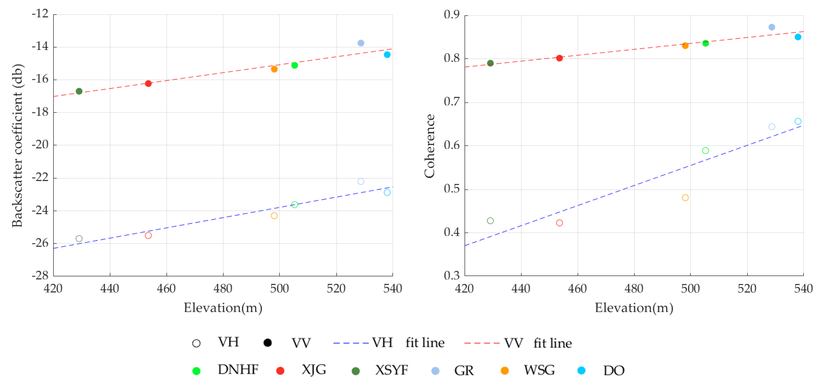
As another important factor that affects backscatter value, the surface roughness is controlled by the topography and the grain size [63]. In this study, as can be seen in Figure 9, the averaged backscatter coefficients and coherence have a close relationship with averaged elevation. Thus, the significant difference (Figure 8 and Table 2) of the mean backscatter coefficients and mean coherence among all rock units might be attributed to the different elevations. However, when we utilize the SAR data to distinguish different rock units, we prefer to exclude or reduce the effect of the topography on the backscatter value and focus more on the rock unit itself. Due to the elevation, the same unit varies. To some extent, the variation of time-series backscatter metrics can suppress the influence of terrain and magnify the impact of the rock unit itself because the elevation does not change over a short period normally. The result demonstrated in Table 4 and Table 6 proved that the time-series Sentinel-1 data could provide better performance than single-date Sentinel-1 data. Similarly, the coherence loss calculated between two consecutive observations may mainly be caused by different responses of rock units to the changes of the external environment and time. Therefore, the coherence can provide an additional gain for the final accuracy (Table 4).
It is also necessary to note that when people determine rock units during fieldwork, people usually refer to the rock-forming period, the stratum information, topography, the surrounding environment, and other interpretive signs, while the remote-sensing based methods mainly consider the properties of the upper layer of the surface. Though previous studies demonstrated that radar signals can penetrate the surface up to meters in an extremely dry environment (P and L bands) [66], compared to the thickness of the stratum, it is still not enough. Moreover, an increase in soil moisture can greatly hinder the penetration depth [67,68,69]. For the rock unit XJG, WSG, and XSYF, there exist severe confusion (Table 3 and Table 5) among these three rock units, though they were formed at different periods. One reason for the misclassification, according to (Table 1) the field survey, is that the major components of these three rock units are similar, and the upper part of these three rock units are usually a layer of loose sediments, including sand, loess, and gravel. The loose structure of the surface layer is easily swept flat by the wind and rainfall. Thus the smooth flat surface reflects away most of the radar signal and results in low backscatter values [68,70]. As the increasing proportion of sand, the backscatter continues to decrease due to the increased attenuation. This explains the lower VV and VH backscatter values of XJG, WSG, and XSYF than that of GR, DNHF, and DO.
A rock unit often encompasses several rock types. Some rock unit comprises the same rock type (e.g., sandstone in DNHF and XJG), and different rock types have similar contents (e.g., SiO2). In our study, granodiorite, as an intrusive rock, is an intermediate between diorite and granite with a semblable appearance to diorite and granite. In terms of composition, granodiorite has more quartz than diorite and more mafic mineral than granite. During the fieldwork, areas with more granite were determined as GR, and areas with more diorite were determined as DO. From the perspective of remote sensing, similar backscatter behaviors also lead to confusion and low accuracy.
The local climate might be another factor that leads to the confusion. As mentioned before, the climate is dry with strong wind, and the large diurnal temperature difference accelerates the disintegration of rock. The effect of weathering is intense. The field survey found that aeolian sand accumulation usually occurs in rugged places. In addition, the resistance to weathering varies, and in most cases, the rock might break into gravel of different sizes. As a consequence, the surface roughness varies, which then leads to different backscatter signals.
Our results showed that polarization VV and VH can provide comparable accuracy (Table 7 and Table 8) and the combined use of VV and VH provided an additional gain for the final accuracy (Table 4). However, compared to the VV, VH yielded a lower coherence, which may be a result of low intensity from the returned radar signal at the VH channel due to the low signal-to-noise ratio [71]. Moreover, according to [35], the backscattered signal dominated by the reflection from the planar surface contributes to maintaining the polarization significantly. In our results (Figure 8), rock units (XJG, WSG, and XSYF) with loose sediments and flat surfaces provided lower backscatter coefficients and coherence at the VH channel than other rock units. This enhances the contrast between the rock units with a strong returned signal and a weak returned signal. Meanwhile, the dry weather can lead to the sand in the upper layer being transparent for the radar signal and result in a volume scattering which explains that the backscatter coefficient VH is more helpful to discriminate rock units with high sand content (e.g., XJG) than VV. As a result, VH polarization, compared to VV, is more sensitive to volume scattering [63].
6. Conclusions
The main aim of this study is to evaluate the potential of time-series SAR metrics derived from Sentinel-1 data for rock unit discrimination. Previous studies have proven that the SAR data can be useful in geology due to its sensitivity to the structure, surface roughness, and dielectric properties. However, most of the studies utilized full polarization SAR or multi-frequency SAR or with other source data. These studies usually focused on using single-date SAR data. To the best of our knowledge, there are no previous studies using time-series SAR data to discriminate rock units.
In this study, we analyzed the temporal variation of the Sentinel-1 derived metrics (backscatter coefficient and coherence) among six rock units from April to October. The result showed that the temporal responses of different rock units were different. This built the prerequisites for the following discrimination based on the combined use of RF algorithm, and time-series Sentinel-1 derived metrics. Before the discrimination, the Kruskal–Wallis rank sum test and Tukey’s HSD test were applied on the SAR metrics, and there exists a significant difference in all time-series SAR metrics derived from Sentinel-1 data among different rock units. However, the Tukey’s HSD test further proved that the significant difference only exists between some of the rock units, such as GR and XJG. At last, RF was used to discriminate the rock unit. The performance of the metrics derived from time-series Sentinel-1 were compared with metrics derived from single-date Sentinel-1. Moreover, the influence of polarization and the potential of coherence and backscatter coefficient were also investigated.
According to the overall accuracy and kappa coefficient, we can conclude that time-series metrics derived from Sentinel-1 can show better performance than metrics derived from single-date Sentinel-1 data (with accuracies of 64.4% and 55.4%, respectively). The influence of polarization is comparable; VV and VH yield similar accuracy. The combined use of VV and VH can improve the final accuracy. The coherence, in this study, provided a slightly worse result than the backscatter coefficient. Even so, the coherence still complements the performance of the backscatter coefficient. Moreover, compared to other rock units, GR and XJG yield higher accuracy.
Although the final result is still not very high, compared to the use of single-date Sentinel-1 data, there is a visible improvement. This study further showed the great potential of time series Sentinel-1 data in the discrimination of rock units. Denser time-series SAR data will be expected in future studies. Moreover, high-resolution SAR datasets such as Radarsat-2 and ALOS-2, which have full polarizations with different inclination angles are also need further analyzed to prove the importance of incorporating time-series SAR for rock unit determination.
Author Contributions
Conceptualization, Y.L.; methodology, Y.L.; validation, Y.L. and C.Y.; formal analysis, Y.L.; writing—original draft preparation, Y.L.; writing—review and editing, Y.L., C.Y. and Q.J.; supervision, C.Y. and Q.J. All authors have read and agreed to the published version of the manuscript.
Funding
This research was funded by the National Remote Sensing Geological Survey of Global Key Zones, Project NO. DD20190536.
Institutional Review Board Statement
Not applicable.
Informed Consent Statement
Not applicable.
Data Availability Statement
Not applicable.
Acknowledgments
The authors thank all those students and teachers from Jilin University who actively participated in the field and laboratory work.
Conflicts of Interest
The authors declare no conflict of interest.
References
- Luo, H.; Lai, F.; Dong, Z.; Xia, W. A lithology identification method for continental shale oil reservoir based on BP neural network. J. Geophys. Eng. 2018, 15, 895–908. [Google Scholar] [CrossRef] [Green Version]
- Adiri, Z.; Lhissou, R.; El Harti, A.; Jellouli, A.; Chakouri, M. Recent advances in the use of public domain satellite imagery for mineral exploration: A review of Landsat-8 and Sentinel-2 applications. Ore Geol. Rev. 2020, 117, 103332. [Google Scholar] [CrossRef]
- Rajan Girija, R.; Mayappan, S. Mapping of mineral resources and lithological units: A review of remote sensing techniques. Int. J. Image Data Fusion 2019, 10, 79–106. [Google Scholar] [CrossRef]
- Schetselaar, E.M.; Chung, C.J.F.; Kim, K.E. Integration of landsat TM, gamma-ray, magnetic, and field data to discriminate lithological units in vegetated granite-gneiss terrain. Remote Sens. Environ. 2000, 71, 89–105. [Google Scholar] [CrossRef]
- Vincent, R.K.; Thomson, F. Spectral Compositional Imaging of Silicate Rock. J. Geophys. Res. 1972, 77, 2465–2472. [Google Scholar] [CrossRef]
- Walter, L.S.; Salisbury, J.W. Spectral characterization of igneous rocks in the 8- to 12-μm region. J. Geophys. Res. 1989, 94, 9203–9213. [Google Scholar] [CrossRef]
- Van Ruitenbeek, F.J.A.; van der Werff, H.M.A.; Bakker, W.H.; van der Meer, F.D.; Hein, K.A.A. Measuring rock microstructure in hyperspectral mineral maps. Remote Sens. Environ. 2019, 220, 94–109. [Google Scholar] [CrossRef]
- Vincent, R.K.; Hunt, G.R. Infrared Reflectance from Mat Surfaces. Appl. Opt. 1968, 7, 53. [Google Scholar] [CrossRef]
- Conel, J.E. Infrared emissivities of silicates: Experimental results and a cloudy atmosphere model of spectral emission from condensed particulate mediums. J. Geophys. Res. 1969, 74, 1614–1634. [Google Scholar] [CrossRef]
- Lyon, R.J.P. Analysis of rocks by spectral infrared emission (8 to 25 microns). Econ. Geol. 1965, 60, 715–736. [Google Scholar] [CrossRef]
- Hunt, G.R.; Salisbury, J.W. Mid-Infrared Spectral Behavior of Sedimentary Rocks; Air Force Cambridge Research Laboratories, Air Force Systems Command, United States Air Force: Cambridge, MA, USA, 1975; Volume 75. [Google Scholar]
- Salisbury, J.W.; Walter, L.S. Thermal infrared (2.5–13.5 μm) spectroscopic remote sensing of igneous rock types on particulate planetary surfaces. J. Geophys. Res. 1989, 94, 9192–9202. [Google Scholar] [CrossRef]
- Salisbury, J.W.; D’Aria, D.M. Emissivity of terrestrial materials in the 3–5 μm atmospheric window. Remote Sens. Environ. 1994, 47, 345–361. [Google Scholar] [CrossRef]
- An, P.; Chung, C.F.; Rencz, A.N. Digital lithology mapping from airborne geophysical and remote sensing data in the Melville Peninsula, Northern Canada, using a neural network approach. Remote Sens. Environ. 1995, 53, 76–84. [Google Scholar] [CrossRef]
- Gad, S.; Kusky, T. ASTER spectral ratioing for lithological mapping in the Arabian-Nubian shield, the Neoproterozoic Wadi Kid area, Sinai, Egypt. Gondwana Res. 2007, 11, 326–335. [Google Scholar] [CrossRef]
- Kumar, C.; Chatterjee, S.; Oommen, T.; Guha, A. Automated lithological mapping by integrating spectral enhancement techniques and machine learning algorithms using AVIRIS-NG hyperspectral data in Gold-bearing granite-greenstone rocks in Hutti, India. Int. J. Appl. Earth Obs. Geoinf. 2020, 86, 102006. [Google Scholar] [CrossRef]
- Fan, Y.H.; Wang, H. Application of remote sensing to identify Copper–Lead–Zinc deposits in the Heiqia area of the West Kunlun Mountains, Chinas. Sci. Rep. 2020, 10, 12309. [Google Scholar] [CrossRef] [PubMed]
- Tan, Y.; Lu, L.; Bruzzone, L.; Guan, R.; Chang, Z.; Yang, C. Hyperspectral Band Selection for Lithologic Discrimination and Geological Mapping. IEEE J. Sel. Top. Appl. Earth Obs. Remote Sens. 2020, 13, 471–486. [Google Scholar] [CrossRef]
- Zhang, X.; Li, P. Lithological mapping from hyperspectral data by improved use of spectral angle mapper. Int. J. Appl. Earth Obs. Geoinf. 2014, 31, 95–109. [Google Scholar] [CrossRef]
- Askari, G.; Pour, A.; Pradhan, B.; Sarfi, M.; Nazemnejad, F. Band Ratios Matrix Transformation (BRMT): A Sedimentary Lithology Mapping Approach Using ASTER Satellite Sensor. Sensors 2018, 18, 3213. [Google Scholar] [CrossRef] [Green Version]
- Jakob, S.; Bühler, B.; Gloaguen, R.; Breitkreuz, C.; Eliwa, H.A.; El Gameel, K. Remote sensing based improvement of the geological map of the Neoproterozoic Ras Gharib segment in the Eastern Desert (NE-Egypt) using texture features. J. Afr. Earth Sci. 2015, 111, 138–147. [Google Scholar] [CrossRef]
- Ge, W.; Cheng, Q.; Tang, Y.; Jing, L.; Gao, C. Lithological Classification Using Sentinel-2A Data in the Shibanjing Ophiolite Complex in Inner Mongolia, China. Remote Sens. 2018, 10, 638. [Google Scholar] [CrossRef] [Green Version]
- Yu, L.; Porwal, A.; Holden, E.J.; Dentith, M.C. Towards automatic lithological classification from remote sensing data using support vector machines. Comput. Geosci. 2012, 45, 229–239. [Google Scholar] [CrossRef]
- Masoumi, F.; Eslamkish, T.; Abkar, A.A.; Honarmand, M.; Harris, J.R. Integration of spectral, thermal, and textural features of ASTER data using Random Forests classification for lithological mapping. J. Afr. Earth Sci. 2017, 129, 445–457. [Google Scholar] [CrossRef]
- Grebby, S.; Cunningham, D.; Naden, J.; Tansey, K. Lithological mapping of the Troodos ophiolite, Cyprus, using airborne LiDAR topographic data. Remote Sens. Environ. 2010, 114, 713–724. [Google Scholar] [CrossRef] [Green Version]
- Yang, M.; Kang, L.; Chen, H.; Zhou, M.; Zhang, J. Lithological mapping of East Tianshan area using integrated data fused by Chinese GF-1 PAN and ASTER multi-spectral data. Open Geosci. 2018, 10, 532–543. [Google Scholar] [CrossRef]
- Bachri, I.; Hakdaoui, M.; Raji, M.; Teodoro, A.C.; Benbouziane, A. Machine Learning Algorithms for Automatic Lithological Mapping Using Remote Sensing Data: A Case Study from Souk Arbaa Sahel, Sidi Ifni Inlier, Western Anti-Atlas, Morocco. ISPRS Int. J. Geo-Inform. 2019, 8, 248. [Google Scholar] [CrossRef] [Green Version]
- Grebby, S.; Naden, J.; Cunningham, D.; Tansey, K. Integrating airborne multispectral imagery and airborne LiDAR data for enhanced lithological mapping in vegetated terrain. Remote Sens. Environ. 2011, 115, 214–226. [Google Scholar] [CrossRef] [Green Version]
- Champatiray, P.K.; Roy, A.K.; Prabhakaran, B. Evaluation and integration of ERS-1-SAR and optical sensor data (TM and IRS) for geological investigations. J. Indian Soc. Remote Sens. 1995, 23, 77–86. [Google Scholar] [CrossRef]
- Mather, P.M.; Tso, B.; Koch, M. An evaluation of Landsat TM spectral data and SAR-derived textural information for lithological discrimination in the Red Sea Hills, Sudan. Int. J. Remote Sens. 1998, 19, 587–604. [Google Scholar] [CrossRef]
- Dong, P.; Leblon, B. Rock unit discrimination on Landsat TM, SIR-C and Radarsat images using spectral and textural information. Int. J. Remote Sens. 2004, 25, 3745–3768. [Google Scholar] [CrossRef]
- Thurmond, A.K.; Abdelsalam, M.G.; Thurmond, J.B. Optical-radar-DEM remote sensing data integration for geological mapping in the Afar Depression, Ethiopia. J. Afr. Earth Sci. 2006, 44, 119–134. [Google Scholar] [CrossRef]
- Pal, M.; Rasmussen, T.; Porwal, A. Optimized Lithological Mapping from Multispectral and Hyperspectral Remote Sensing Images Using Fused Multi-Classifiers. Remote Sens. 2020, 12, 177. [Google Scholar] [CrossRef] [Green Version]
- Dellwig, L.F.; Moore, R.K. The geological value of simultaneously produced like- and cross-polarized radar imagery. J. Geophys. Res. 1966, 71, 3597–3601. [Google Scholar] [CrossRef]
- Mccauley, J.R. Surface configuration as an explanation for lithology-related cross-polarized radar image anomalies. NASA STI/Recon Tech. Rep. N 1973, 75, 18642. [Google Scholar]
- He, D.C.; Wang, L. Recognition of lithological units in airborne SAR images using new texture features. Int. J. Remote Sens. 1990, 11, 2337–2344. [Google Scholar] [CrossRef]
- Lu, Y.; Yang, C.; Meng, Z. Lithology discrimination using Sentinel-1 dual-pol data and SRTM data. Remote Sens. 2021, 13, 1280. [Google Scholar] [CrossRef]
- Wang, C.; Guo, H.; Shao, Y. Lithological classification in mountain area with polarimetric decomposition. In Proceedings of the International Geoscience and Remote Sensing Symposium (IGARSS), Seattle, WA, USA, 6–10 July 1998; Volume 3, pp. 1342–1344. [Google Scholar]
- Xie, M.; Zhang, Q.; Chen, S.; Zha, F. A lithological classification method from fully polarimetric SAR data using Cloude-Pottier decomposition and SVM. In Proceedings of the AOPC 2015: Optical and Optoelectronic Sensing and Imaging Technology, Beijing, China, 5–7 May 2015; Volume 9674, p. 967405. [Google Scholar]
- Da Silva, A.; Paradella, W.; Freitas, C.; Oliveira, C. Evaluation of Digital Classification of Polarimetric SAR Data for Iron-Mineralized Laterites Mapping in the Amazon Region. Remote Sens. 2013, 5, 3101–3122. [Google Scholar] [CrossRef] [Green Version]
- Wang, W.; Ren, X.; Zhang, Y.; Li, M. Deep Learning Based Lithology Classification Using Dual-Frequency Pol-SAR Data. Appl. Sci. 2018, 8, 1513. [Google Scholar] [CrossRef] [Green Version]
- Guo, H.; Zhu, L.; Shao, Y.; Lu, X. Detection of structural and lithological features underneath a vegetation canopy using SIR-C/X-SAR data in Zhao Qing test site of southern China. J. Geophys. Res. E Planets 1996, 101, 23101–23108. [Google Scholar] [CrossRef]
- Radford, D.D.G.; Cracknell, M.J.; Roach, M.J.; Cumming, G.V. Geological Mapping in Western Tasmania Using Radar and Random Forests. IEEE J. Sel. Top. Appl. Earth Obs. Remote Sens. 2018, 11, 3075–3087. [Google Scholar] [CrossRef]
- Ichoku, C.; Karnieli, A.; Arkin, Y.; Chorowicz, J.; Fleury, T.; Rudant, J.-P. Exploring the utility potential of SAR interferometric coherence images. Int. J. Remote Sens. 1998, 19, 1147–1160. [Google Scholar] [CrossRef]
- Galford, G.L.; Mustard, J.F.; Melillo, J.; Gendrin, A.; Cerri, C.C.; Cerri, C.E.P. Wavelet analysis of MODIS time series to detect expansion and intensification of row-crop agriculture in Brazil. Remote Sens. Environ. 2008, 112, 576–587. [Google Scholar] [CrossRef]
- Picoli, M.C.A.; Camara, G.; Sanches, I.; Simões, R.; Carvalho, A.; Maciel, A.; Coutinho, A.; Esquerdo, J.; Antunes, J.; Begotti, R.A.; et al. Big earth observation time series analysis for monitoring Brazilian agriculture. ISPRS J. Photogramm. Remote Sens. 2018, 145, 328–339. [Google Scholar] [CrossRef]
- Chen, B.; Xiao, X.; Li, X.; Pan, L.; Doughty, R.; Ma, J.; Dong, J.; Qin, Y.; Zhao, B.; Wu, Z.; et al. A mangrove forest map of China in 2015: Analysis of time series Landsat 7/8 and Sentinel-1A imagery in Google Earth Engine cloud computing platform. ISPRS J. Photogramm. Remote Sens. 2017, 131, 104–120. [Google Scholar] [CrossRef]
- Cai, Y.; Lin, H.; Zhang, M. Mapping paddy rice by the object-based random forest method using time series Sentinel-1/Sentinel-2 data. Adv. Spaces Res. 2019, 64, 2233–2244. [Google Scholar] [CrossRef]
- Dai, K.; Li, Z.; Tomás, R.; Liu, G.; Yu, B.; Wang, X.; Cheng, H.; Chen, J.; Stockamp, J. Monitoring activity at the Daguangbao mega-landslide (China) using Sentinel-1 TOPS time series interferometry. Remote Sens. Environ. 2016, 186, 501–513. [Google Scholar] [CrossRef] [Green Version]
- Pawluszek-Filipiak, K.; Borkowski, A. Integration of DInSAR and SBAS Techniques to Determine Mining-Related Deformations Using Sentinel-1 Data: The Case Study of Rydułtowy Mine in Poland. Remote Sens. 2020, 12, 242. [Google Scholar] [CrossRef] [Green Version]
- Gagliardi, V.; Bianchini Ciampoli, L.; Trevisani, S.; D’amico, F.; Alani, A.M.; Benedetto, A.; Tosti, F. Testing sentinel-1 sar interferometry data for airport runway monitoring: A geostatistical analysis. Sensors 2021, 21, 5769. [Google Scholar] [CrossRef] [PubMed]
- Mestre-Quereda, A.; Lopez-Sanchez, J.M.; Vicente-Guijalba, F.; Jacob, A.W.; Engdahl, M.E. Time-Series of Sentinel-1 Interferometric Coherence and Backscatter for Crop-Type Mapping. IEEE J. Sel. Top. Appl. Earth Obs. Remote Sens. 2020, 13, 4070–4084. [Google Scholar] [CrossRef]
- Ullmann, T.; Stauch, G. Surface roughness estimation in the orog nuur basin (Southern mongolia) using sentinel-1 SAR time series and ground-based photogrammetry. Remote Sens. 2020, 12, 3200. [Google Scholar] [CrossRef]
- Ghafouri, A.; Amini, J.; Dehmollaian, M.; Kavoosi, M.A. Measuring the surface roughness of geological rock surfaces in SAR data using fractal geometry. Comptes Rendus Geosci. 2017, 349, 114–125. [Google Scholar] [CrossRef]
- El Hajj, M.; Baghdadi, N.; Belaud, G.; Zribi, M.; Cheviron, B.; Courault, D.; Hagolle, O.; Charron, F. Irrigated Grassland Monitoring Using a Time Series of TerraSAR-X and COSMO-SkyMed X-Band SAR Data. Remote Sens. 2014, 6, 10002–10032. [Google Scholar] [CrossRef] [Green Version]
- Deng, X.H.; Wang, J.B.; Pirajno, F.; Mao, Q.G.; Long, L.L. A review of Cu-dominant mineral systems in the Kalatag district, East Tianshan, China. Ore Geol. Rev. 2020, 117, 103284. [Google Scholar] [CrossRef]
- Xinjiang Uygur Autonomous Region Regional Stratigraphic Table Compilation Group. Regional Stratigraphic Table of Northwest China Xinjiang Uygur Autonomous Region; Geological Publishing House: Beijing, China, 1981. [Google Scholar]
- Filipponi, F. Sentinel-1 GRD Preprocessing Workflow. Proceedings 2019, 18, 11. [Google Scholar] [CrossRef] [Green Version]
- Zebker, H.A.; Villasenor, J. Decorrelation in interferometric radar echoes. IEEE Trans. Geosci. Remote Sens. 1992, 30, 950–959. [Google Scholar] [CrossRef] [Green Version]
- Kruskal, W.H.; Wallis, W.A. Use of Ranks in One-Criterion Variance Analysis. J. Am. Stat. Assoc. 1952, 47, 583–621. [Google Scholar] [CrossRef]
- Breiman, L. Random Forests. Mach. Learn. 2001, 45, 5–32. [Google Scholar] [CrossRef] [Green Version]
- O’Grady, D.; Leblanc, M.; Bass, A. The use of radar satellite data from multiple incidence angles improves surface water mapping. Remote Sens. Environ. 2014, 140, 652–664. [Google Scholar] [CrossRef]
- Gaber, A.; Soliman, F.; Koch, M.; El-Baz, F. Using full-polarimetric SAR data to characterize the surface sediments in desert areas: A case study in El-Gallaba Plain, Egypt. Remote Sens. Environ. 2015, 162, 11–28. [Google Scholar] [CrossRef]
- Huang, S.; Ding, J.; Zou, J.; Liu, B.; Zhang, J.; Chen, W. Soil moisture retrival based on sentinel-1 imagery under sparse vegetation coverage. Sensors 2019, 19, 589. [Google Scholar] [CrossRef] [Green Version]
- Molijn, R.A.; Iannini, L.; Dekker, P.L.; Magalhães, P.S.G.; Hanssen, R.F. Vegetation characterization through the use of precipitation-affected SAR signals. Remote Sens. 2018, 10, 1647. [Google Scholar] [CrossRef] [Green Version]
- Gaber, A.; Amarah, B.A.; Abdelfattah, M.; Ali, S. Investigating the use of the dual-polarized and large incident angle of SAR data for mapping the fluvial and aeolian deposits. NRIAG J. Astron. Geophys. 2017, 6, 349–360. [Google Scholar] [CrossRef] [Green Version]
- Gorrab, A.; Zribi, M.; Baghdadi, N.; Mougenot, B. Multi-frequency analysis of soil moisture vertical heterogeneity effect on radar backscatter. In Proceedings of the 1st International Conference on Advanced Technologies for Signal and Image Processing (ATSIP), Sousse, Tunisia, 17–19 March 2014; pp. 379–384. [Google Scholar]
- Williams, K.K.; Greeley, R. Laboratory and field measurements of the modification of radar backscatter by sand. Remote Sens. Environ. 2004, 89, 29–40. [Google Scholar] [CrossRef]
- Morrison, K.; Wagner, W. Explaining Anomalies in SAR and Scatterometer Soil Moisture Retrievals from Dry Soils with Subsurface Scattering. IEEE Trans. Geosci. Remote Sens. 2020, 58, 2190–2197. [Google Scholar] [CrossRef] [Green Version]
- Abdelsalam, M.G.; Robinson, C.; El-Baz, F.; Stern, R.J. Applications of orbital imaging radar for geologic studies in arid regions: The Saharan testimony. Photogramm. Eng. Remote Sens. 2000, 66, 717–726. [Google Scholar]
- Jacob, A.W.; Notarnicola, C.; Suresh, G.; Antropov, O.; Ge, S.; Praks, J.; Ban, Y.; Pottier, E.; Mallorqui Franquet, J.J.; Duro, J.; et al. Sentinel-1 InSAR Coherence for Land Cover Mapping: A Comparison of Multiple Feature-Based Classifiers. IEEE J. Sel. Top. Appl. Earth Obs. Remote Sens. 2020, 13, 535–552. [Google Scholar] [CrossRef] [Green Version]
Figure 1.
(a) Study area (the background is a mosaic Sentinel-2 image acquired around June 2020) and field survey sample distribution; (b) photos of typical lithology found during the fieldwork.
Figure 1.
(a) Study area (the background is a mosaic Sentinel-2 image acquired around June 2020) and field survey sample distribution; (b) photos of typical lithology found during the fieldwork.

Figure 2.
Monthly average precipitation, snowfall, and temperature throughout the year (Source: worldweatheronline.com, accessed on 10 October 2021).
Figure 2.
Monthly average precipitation, snowfall, and temperature throughout the year (Source: worldweatheronline.com, accessed on 10 October 2021).

Figure 3.
Acquisition Date of Sentinel-1 products.

Figure 4.
Methodological flowchart of this study.

Figure 5.
Temporal average backscatter coefficient at (a) VH and (b) VV channels of different rock units.
Figure 5.
Temporal average backscatter coefficient at (a) VH and (b) VV channels of different rock units.

Figure 6.
Temporal variation of VH coherence of different rock units.

Figure 7.
Temporal variation of VV coherence of different rock units.

Figure 8.
Box plots of variations of (a) Sentinel-1 backscatter coefficients at VV channel, (b) Sentinel-1 backscatter coefficients at VH channel, (c) Sentinel-1 coherence at VV channel and (d) Sentinel-1 coherence at VH channel (n = DNHF:43, GR:67, XJG:208, WSG:25, XSYF:73, DO:35). The mean value of each box is represented by the black circle.

Figure 9.
The relationship between averaged elevation and the averaged backscatter metrics of the six rock units (the elevation data is obtained from SRTM).
Figure 9.
The relationship between averaged elevation and the averaged backscatter metrics of the six rock units (the elevation data is obtained from SRTM).


Table 1.
Detailed information of the rock units in the study area.
| Rock Unit | Abbreviation | Major Component | Period |
|---|---|---|---|
| Dananhu Formation | DNHF | basalt-tuff, breccia, limestone, sandstone, mable, andesitic porphyrite, dacite porphyry, andesite-basalt | Devonian |
| Granite | GR | granite, granodiorite | Carboniferous |
| Xinjiang Group | XJG | alluvial and fluvial layer | Quaternary upper pleistocene |
| Wusu Group | WSG | sandstone, loess, gravel | Quaternary middle pleistocene |
| Xishanyao Formation | XSYF | sandstone, mudstone, and coal | Jurassic |
| Diorite | DO | diorite, granodiorite | Carboniferous |
Table 2.
Results of Kruskal–Wallis rank sum test.
| Polarization Parameters | p-Value |
|---|---|
| VH | 7.286 × 10⁻³² |
| VV | 3.285 × 10⁻²⁶ |
| Coherence VH | 9.138 × 10−38 |
| Coherence VV | 3.499 × 10⁻¹⁸ |
Table 3.
Results of Tukey’s HSD test. * and ** represent the statistical variances at 95% and 99% confidence levels.
Table 3.
Results of Tukey’s HSD test. * and ** represent the statistical variances at 95% and 99% confidence levels.
| Pairwise Group | p-Value | ||||
|---|---|---|---|---|---|
| Group1 | Group2 | VV | VH | Coh VV | Coh VH |
| DNHF | GR | 0.0005 ** | 0.0021 ** | 0.0499 * | 0.1283 |
| DNHF | XJG | 0.0011 ** | 0.0000 ** | 0.0258 | 0.0000 ** |
| DNHF | WSG | 0.9944 | 0.7209 | 0.9995 | 0.0020 ** |
| DNHF | XSYF | 0.0000 ** | 0.0001 ** | 0.0045 | 0.0000 ** |
| DNHF | GD | 0.5227 | 0.5304 | 0.9312 | 0.0943 |
| GR | XJG | 0.0000 ** | 0.0000 ** | 0.0000 ** | 0.0000 ** |
| GR | WSG | 0.0000 ** | 0.0000 ** | 0.0687 | 0.0000 ** |
| GR | XSYF | 0.0000 ** | 0.0000 ** | 0.0000 ** | 0.0000 ** |
| GR | GD | 0.3310 | 0.5351 | 0.5817 | 0.9953 |
| XJG | WSG | 0.1296 | 0.0339 * | 0.3214 | 0.1490 |
| XJG | XSYF | 0.3110 | 0.9772 | 0.7951 | 0.9996 |
| XJG | GD | 0.0000 ** | 0.0000 ** | 0.0009 | 0.0000 ** |
| WSG | XSYF | 0.0068 ** | 0.0198 * | 0.0941 | 0.3290 |
| WSG | GD | 0.3356 | 0.0522 | 0.8592 | 0.0000 ** |
| XSYF | GD | 0.0000 ** | 0.0000 ** | 0.0001 ** | 0.0000 ** |
Table 4.
Accuracy assessment of the result using time-series backscatter coefficient, coherence, and both backscatter coefficient and coherence.
Table 4.
Accuracy assessment of the result using time-series backscatter coefficient, coherence, and both backscatter coefficient and coherence.
| Backscatter Coefficient | Coherence | Backscatter Coefficient and Coherence | |||||||
|---|---|---|---|---|---|---|---|---|---|
| Rock Unit | Precision | Recall | F1-Score | Precision | Recall | F1-Score | Precision | Recall | F1-Score |
| DNHF | 26% | 7% | 0.11 | 47% | 9% | 0.15 | 34% | 10% | 0.15 |
| GR | 63% | 72% | 0.67 | 58% | 58% | 0.58 | 67% | 71% | 0.69 |
| XJG | 69% | 90% | 0.78 | 66% | 90% | 0.76 | 69% | 91% | 0.78 |
| WSG | 46% | 10% | 0.16 | 81% | 8% | 0.14 | 68% | 9% | 0.16 |
| XSYF | 16% | 7% | 0.10 | 30% | 8% | 0.13 | 16% | 6% | 0.09 |
| DO | 26% | 15% | 0.19 | 32% | 36% | 0.34 | 37% | 33% | 0.35 |
| Kappa | 0.373 | 0.337 | 0.390 | ||||||
| OA | 63.3% | 61.8% | 64.4% | ||||||
Table 5.
The normalized confusion matrix uses the backscatter coefficient and coherence as input features.
Table 5.
The normalized confusion matrix uses the backscatter coefficient and coherence as input features.
| Ground Truth | |||||||
|---|---|---|---|---|---|---|---|
| DNHF | GR | XJG | WSG | XSYF | DO | ||
| Predicted | DNHF | 0.10 | 0.04 | 0.02 | 0.01 | 0.01 | 0.05 |
| GR | 0.29 | 0.71 | 0.02 | 0.04 | 0.07 | 0.37 | |
| XJG | 0.51 | 0.18 | 0.91 | 0.86 | 0.86 | 0.24 | |
| WSG | 0.01 | 0.00 | 0.00 | 0.09 | 0.00 | 0.00 | |
| XSYF | 0.03 | 0.01 | 0.05 | 0.00 | 0.06 | 0.00 | |
| DO | 0.05 | 0.06 | 0.02 | 0.00 | 0.00 | 0.33 | |
Table 6.
Accuracy assessment of the result using backscatter coefficient (accessed on 28 May), coherence (accessed on 16 May and 28 May), and both backscatter coefficient and coherence.
Table 6.
Accuracy assessment of the result using backscatter coefficient (accessed on 28 May), coherence (accessed on 16 May and 28 May), and both backscatter coefficient and coherence.
| Backscatter Coefficient | Coherence | Backscatter Coefficient and Coherence | |||||||
|---|---|---|---|---|---|---|---|---|---|
| Rock Unit | Precision | Recall | F1-Score | Precision | Recall | F1-Score | Precision | Recall | F1-Score |
| DNHF | 17% | 7% | 0.10 | 20% | 9% | 0.13 | 24% | 8% | 0.11 |
| GR | 52% | 45% | 0.48 | 45% | 35% | 0.39 | 57% | 52% | 0.54 |
| XJG | 66% | 72% | 0.69 | 64% | 71% | 0.67 | 66% | 81% | 0.73 |
| WSG | 20% | 12% | 0.15 | 17% | 10% | 0.12 | 32% | 11% | 0.16 |
| XSYF | 11% | 13% | 0.12 | 11% | 15% | 0.12 | 11% | 10% | 0.10 |
| DO | 11% | 16% | 0.13 | 12% | 20% | 0.15 | 18% | 21% | 0.19 |
| Kappa | 0.215 | 0.181 | 0.267 | ||||||
| OA | 50.0% | 47.6% | 55.4% | ||||||
Table 7.
Accuracy assessment of the result using time-series backscatter coefficient, coherence, and both backscatter coefficient and coherence at VV channel.
Table 7.
Accuracy assessment of the result using time-series backscatter coefficient, coherence, and both backscatter coefficient and coherence at VV channel.
| Backscatter Coefficient | Coherence | Backscatter Coefficient and Coherence | |||||||
|---|---|---|---|---|---|---|---|---|---|
| Rock Unit | Precision | Recall | F1-Score | Precision | ReCall | F1-Score | Precision | Recall | F1-Score |
| DNHF | 48% | 5% | 0.09 | 48% | 10% | 0.17 | 72% | 6% | 0.12 |
| GR | 57% | 64% | 0.61 | 58% | 50% | 0.53 | 63% | 64% | 0.64 |
| XJG | 67% | 89% | 0.77 | 63% | 87% | 0.73 | 66% | 91% | 0.77 |
| WSG | 68% | 10% | 0.17 | 61% | 8% | 0.14 | 91% | 12% | 0.22 |
| XSYF | 16% | 8% | 0.11 | 32% | 16% | 0.21 | 24% | 10% | 0.14 |
| DO | 20% | 15% | 0.17 | 38% | 33% | 0.36 | 38% | 31% | 0.34 |
| Kappa | 0.331 | 0.293 | 0.361 | ||||||
| OA | 61.0% | 59.6% | 63.3% | ||||||
Table 8.
Accuracy assessment of the result using time-series backscatter coefficient, coherence, and both backscatter coefficient and coherence at VH channel.
Table 8.
Accuracy assessment of the result using time-series backscatter coefficient, coherence, and both backscatter coefficient and coherence at VH channel.
| Backscatter Coefficient | Coherence | Backscatter Coefficient and Coherence | |||||||
|---|---|---|---|---|---|---|---|---|---|
| Rock Unit | Precision | Recall | F1-Score | Precision | Recall | F1-Score | Precision | Recall | F1-Score |
| DNHF | 25% | 9% | 0.13 | 32% | 7% | 0.12 | 28% | 9% | 0.13 |
| GR | 64% | 69% | 0.66 | 52% | 50% | 0.51 | 67% | 67% | 0.67 |
| XJG | 69% | 87% | 0.77 | 65% | 89% | 0.75 | 68% | 90% | 0.78 |
| WSG | 49% | 10% | 0.16 | 73% | 8% | 0.14 | 70% | 9% | 0.16 |
| XSYF | 11% | 6% | 0.08 | 15% | 3% | 0.04 | 13% | 5% | 0.07 |
| DO | 27% | 19% | 0.22 | 21% | 25% | 0.23 | 34% | 34% | 0.34 |
| Kappa | 0.351 | 0.285 | 0.370 | ||||||
| OA | 61.3% | 59.0% | 63.1% | ||||||
Publisher’s Note: MDPI stays neutral with regard to jurisdictional claims in published maps and institutional affiliations. |
© 2021 by the authors. Licensee MDPI, Basel, Switzerland. This article is an open access article distributed under the terms and conditions of the Creative Commons Attribution (CC BY) license (https://creativecommons.org/licenses/by/4.0/).
Share and Cite
MDPI and ACS Style
Lu, Y.; Yang, C.; Jiang, Q. Evaluation of the Performance of Time-Series Sentinel-1 Data for Discriminating Rock Units. Remote Sens. 2021, 13, 4824. https://0-doi-org.brum.beds.ac.uk/10.3390/rs13234824
AMA Style
Lu Y, Yang C, Jiang Q. Evaluation of the Performance of Time-Series Sentinel-1 Data for Discriminating Rock Units. Remote Sensing. 2021; 13(23):4824. https://0-doi-org.brum.beds.ac.uk/10.3390/rs13234824
Chicago/Turabian StyleLu, Yi, Changbao Yang, and Qigang Jiang. 2021. "Evaluation of the Performance of Time-Series Sentinel-1 Data for Discriminating Rock Units" Remote Sensing 13, no. 23: 4824. https://0-doi-org.brum.beds.ac.uk/10.3390/rs13234824
Note that from the first issue of 2016, this journal uses article numbers instead of page numbers. See further details here.