
Lithological Mapping Based on Fully Convolutional Network and Multi-Source Geological Data


State Key Laboratory of Geological Processes and Mineral Resources, China University of Geosciences, Wuhan 430074, China
*
Author to whom correspondence should be addressed.
Remote Sens. 2021, 13(23), 4860; https://0-doi-org.brum.beds.ac.uk/10.3390/rs13234860
Submission received: 30 October 2021
/
Revised: 26 November 2021
/
Accepted: 27 November 2021
/
Published: 30 November 2021
(This article belongs to the Special Issue Surface Mineral Allocation and Lithological Mapping Based on Remote Sensing)
Abstract
:Deep learning algorithms have found numerous applications in the field of geological mapping to assist in mineral exploration and benefit from capabilities such as high-dimensional feature learning and processing through multi-layer networks. However, there are two challenges associated with identifying geological features using deep learning methods. On the one hand, a single type of data resource cannot diagnose the characteristics of all geological units; on the other hand, deep learning models are commonly designed to output a certain class for the whole input rather than segmenting it into several parts, which is necessary for geological mapping tasks. To address such concerns, a framework that comprises a multi-source data fusion technology and a fully convolutional network (FCN) model is proposed in this study, aiming to improve the classification accuracy for geological mapping. Furthermore, multi-source data fusion technology is first applied to integrate geochemical, geophysical, and remote sensing data for comprehensive analysis. A semantic segmentation-based FCN model is then constructed to determine the lithological units per pixel by exploring the relationships among multi-source data. The FCN is trained end-to-end and performs dense pixel-wise prediction with an arbitrary input size, which is ideal for targeting geological features such as lithological units. The framework is finally proven by a comparative study in discriminating seven lithological units in the Cuonadong dome, Tibet, China. A total classification accuracy of 0.96 and a high mean intersection over union value of 0.9 were achieved, indicating that the proposed model would be an innovative alternative to traditional machine learning algorithms for geological feature mapping.

1. Introduction
As a fundamental work in mineral exploration, geological mapping plays a crucial role by enabling the detection of geological features that involve lithological units and alterations. Several approaches have been applied for geological mapping to assist in the discovery of mineral deposits based on geological, geophysical, geochemical, and remote sensing data. These methods can be summarized as traditional field surveys, statistical processes, and more recent machine learning technologies (e.g., random forest, support vector machine, and logistic regression) [1,2,3,4]. For example, Wang et al. [5] designed a hybrid method that comprises random forest and metric learning to delineate the spatial distribution of Himalayan leucogranites based on remote sensing images and geochemical data. This approach integrated the advantages of both geochemical and remote sensing, which is helpful for improving the recognition accuracy of Himalayan leucogranite.
As an essential part of machine learning algorithms with multiple hidden layers, deep learning algorithms have emerged as state-of-the-art methods for many important breakthroughs and have garnered increasing interest in the fields of pattern recognition, computer vision, and mineral prospectivity mapping [6,7,8,9,10,11,12,13,14]. Deep learning algorithms are dominant in dealing with high-dimensional datasets for classification and prediction through multi-layer network learning [15]. Taking a convolutional neural network (CNN) as an example, it is a type of feedforward neural network that contains convolution computation and a depth structure. CNN is popular in mineral exploration based on its shared-weights architecture and translation invariance, which can extract inner relationships from complex geological features, explore hidden metallogenic information, and describe the patterns that may be ignored by traditional machine learning methods [12,16,17,18].
However, several difficulties arise associated with the identification of geological features using deep learning models. First, a single type of data resource cannot diagnose the characteristics of all lithological units. Second, commonly used deep learning algorithms require large amounts of known labels, whereas most of the current training datasets are built for 2D images with a fixed input size (e.g., MNIST, ImageNet, and CIFAR-10). Third, for lithological mapping, rather than outputting a certain class, segmenting the input image into several lithological units is required. Compared with traditional image-wise classification, a solution based on CNN tends to take a patch with each pixel as the center, assigns labels to this patch, and predicts the class centered at the corresponding patch based on the information from the whole patch. However, it is difficult to optimize the size of the patch, which determines the learning ability, and the segmentation of training images in lithological units of varying shapes, especially at the overlapping geological boundaries, yields to the classification performance owing to the redundant calculations on the overlapped and neighboring patches [19].
Geodata science, which is defined by analyzing the spatial associations between geological big data and known geoknowledge, is growing in acceptance and being used in geoscience [20,21]. Geodata involves geological, geophysical, geochemical, and remote sensing data, extending from the surface to the depth of the earth to reveal the characteristics of geological features. For example, remote sensing images record electromagnetic waves, characterized by their wide view and high resolution; geochemical data indicate the enrichment and depletion of geochemical elements; and geophysical data reflect the gravity, permeability, conductivity, and radioactivity that can be assessed to explore hidden information under the earth. For the first problem, the incorporation of multi-source geodata is considered an effective and inexpensive approach for the comprehensive analysis of various geodata, especially in areas with limited geological data [5,22,23,24,25].
Mineralization is a typical rare geological event that results in far fewer labeled samples for training deep neural networks [20]. Data augmentation, by the means of flipping, rotation, and clipping, is often recommended to generate additional data for model training. However, these transformations carried on geodata may change the geological meaning of the training labels [12]. The recently-developed fully convolutional network (FCN) provides an alternative solution to such problems. FCN is a semantic segmentation model that trains end-to-end and performs dense per-pixel prediction at an arbitrarily sized input image or labeled pixels, rather than a fixed input 2D/3D image size [26,27,28,29,30]. FCN abandons any of the fully connected layers at the end and only performs convolution operations to predict a class at each pixel of the input image, instead of only one class for the whole input. As a result, FCN can fully utilize limited labels and free from huge computational cost compared with the traditional image-wise or patch-wise classification in CNN [27]. Furthermore, FCN has a capability to deeply understand the nonlinear complex relationship between multi-source geological data. In this case, the application of FCN facilitates the accuracy improvement of lithological boundaries, and therefore, is considered to be favorable for high-precision geological feature mapping.
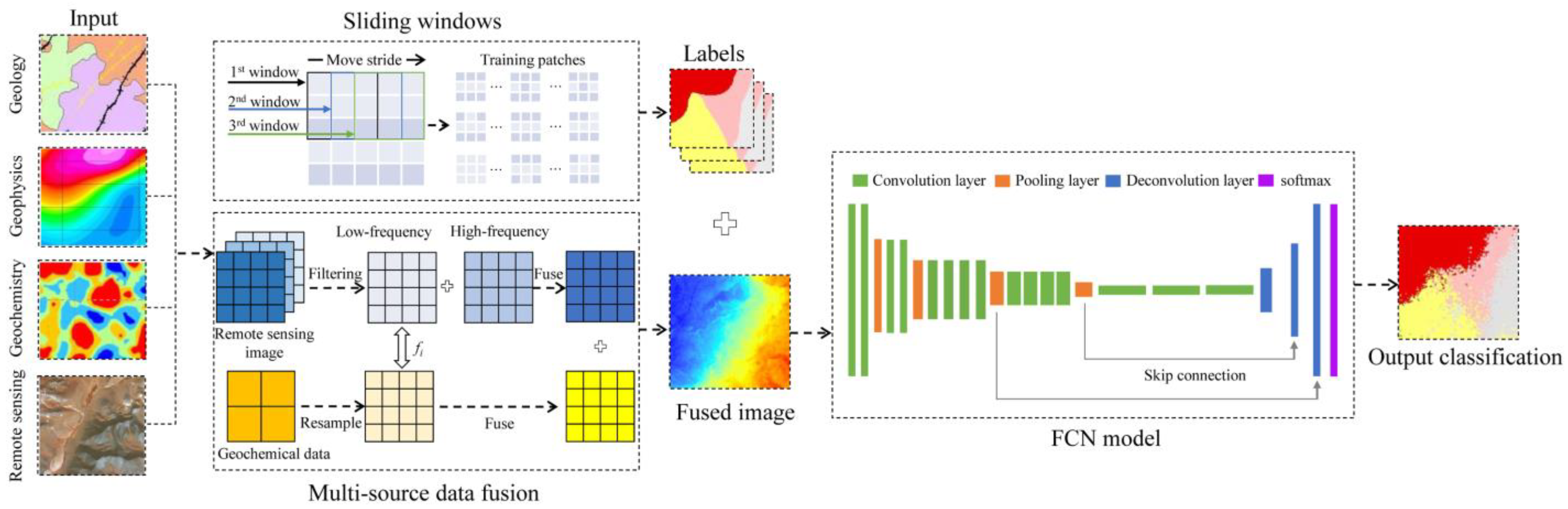
Accordingly, this study aims to develop a promising framework (Figure 1) for lithological mapping, which provides available access to aid decision-making in targeting mineral deposits. Multi-source data fusion technology was first adopted to achieve a comprehensive analysis of geodata by integrating ASTER remote sensing images, PALSAR DEM data, geochemical exploration data, and aeromagnetic data at various scales. An FCN model motivated by the VGG-19 network was then developed to learn the global, local, and contextual features of the fused geodata for lithological mapping. A comparative study to discriminate among several lithological units in the Cuonadong dome, Tibet, China, was conducted to demonstrate the proposed framework, where researchers have discovered rare earth polymetallic mineralization (Be, Li, Ni, Ta, Bi, and Cs) in the Himalayan leucogranite within this area.
2. Methods
2.1. Multi-Source Data Fusion
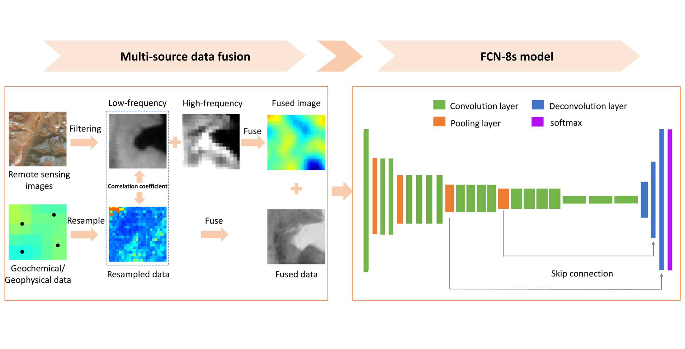
A multispectral remote sensing image can be decomposed into high-frequency components (MS_bHi) and low-frequency components (MS_bLi) by image filtering algorithms, representing the spatial detail and background information, respectively. The distribution of geochemical elements refers to a series of physical processes, such as electronic transitions and atomic vibrations. These processes result in changes in spectral reflection that can be detected and recorded by remote sensing image sensors. In this regard, the mineral spectrum is the response to its chemical and physical components; hence, the low-frequency components of multispectral bands are spatially and genetically related to geochemical or geophysical information (geo), which can be calculated as [31]:
where fi is the correlation coefficient between multispectral bands and geochemical or geophysical information, and bLi denotes the i band of the low-frequency component of the multispectral data.
The low-resolution geochemical or geophysical data can be fused by the reconstructed high-frequency component using the correlation coefficient above:
where geof is the fused high-resolution image, geoc is the resampled geochemical or geophysical data with the same resolution as the high-frequency component, and bLi is the i band of the high-frequency component of the multispectral data.
2.2. Fully Convolutional Network
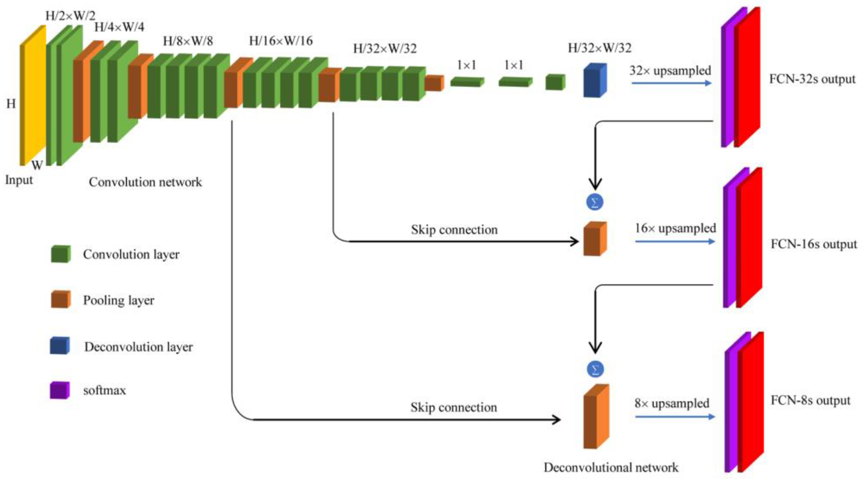
FCN was developed on the basis of a classical CNN and was initially designed for pixel-wise image semantic segmentation [26,32,33]. Semantic segmentation, known as dense classification, aims to classify the category of each pixel in an image according to the annotation. A simple FCN architecture is composed of convolution layers, pool layers, and deconvolution layers that are connected by activation functions, such as the sigmoid, ReLU, and Tanh functions. Figure 2 shows the visualization of the FCN architecture, where the first part is a convolution network similar to a CNN, and the second part is a deconvolution network with skip connection. In more detail, the convolution layer is designed as a feature extraction layer to learn multi-layer features and extract abstract and advanced information from the input data. The pooling layer helps transform high-dimensional features into low-dimensional representative features, thereby reducing the spatial size and computing parameters. Regarding the deconvolution layer, it can be regarded as the reverse process of the convolution layer and the pooling layer, which increases the size of the feature maps by fusing multi-scale global and local feature information with skip connection.
- (1)
- Deconvolution network
In a CNN, the convolutional operation decreases both the size and resolution of the feature image. To recover the size of the feature map as input, the FCN replaces all of the last fully connected layers of the CNN with a 1 × 1 convolution layer. The deconvolution network enables the feature map obtained by the convolution and pooling layers to be restored to the original resolution by a continuous upsampling operation, also called bilinear interpolation. This ingenious operation causes each predicted value to correspond to the pixel in the input image one by one and achieves end-to-end and per-pixel classification [35,36].
- (2)
- Skip connection
The FCN also takes advantage of skip connections to recover lost detailed information during the downsampling operation [27]. Skip connections combine information from the lower and higher layers iteratively, thereby supplementing fine details in the lower layers for the global feature in the higher layers. As shown in Figure 2, the output feature map is obtained by upsampling 32 times directly after the convolution operation; this network is called FCN-32s. When the step size of the deconvolution is set to 16, the output feature map is upsampled 16 times, and connected with the corresponding pooled map, this network is called FCN-8s. A further skip is added to make predictions based on the feature map after 8× upsampling, which is called FCN-8s [26].
2.3. Workflow and FCN Model Architecture
An FCN-8s framework (Figure 1) was constructed for lithological mapping in this study. The implemented FCN-8s model was developed from the well-known VGG-19 network. VGG-19 is an excellent CNN model developed by the visual geometry group of Oxford University, including 16 convolutional layers, 5 max-pooling layers, and 3 fully connected layers, each of which is followed by ReLU as a nonlinear activation function (Table 1) [36]. VGG-19 is capable of reducing the number of parameters and retaining more subtle feature information by stacking multiple smaller-size convolution kernels (3 × 3) and max-pooling kernels (2 × 2), which contributes to the fitting of the nonlinear structure of data, which makes the network more robust. Moreover, the padding technique, a process of adding layers of zeros to the input images, is used in VGG-19 to restore the spatial resolution of the feature map. The FCN-8s model discards the last three fully connected layers and replaces them by convolutional layers with a 1 × 1 sized filter. This special design ensures that the output map keeps the same size as the original input map through two 2 × 2 deconvolutional layers and one with a step size of 8. The FCN-8s model performs pixel-wise prediction using the SoftMax classifier, where the final classification map is obtained by fusing the output abstracted high-level information with fine low-level information from the third and fourth pooling layer using a skip connection [26].
2.4. Model Evaluation Metrics
The confusion matrix and intersection over union (IoU) values were employed to evaluate the performance of the proposed model. A confusion matrix is a summarized table used to quantitatively measure the classification accuracy of each variable and provide a holistic view of how well a classification model is performing [37,38]. The confusion matrix describes the visual representation of the actual labels and predicted values, and where it makes misclassifications by calculating the pixel accuracy.
IoU is a standard metric for segmentation assessment that is specially designed to evaluate how close the predicted value is to the labeled reference [39]. IoU is simply calculated through an overlapping ratio between the predictions and labels (intersection) over their total surface (union) [40]. In addition, the mean IoU (mIoU) is more commonly accepted by considering the average IoU of each class. Generally, the greater the mIoU, the better the model performs.
3. Case Study
3.1. Geological Setting
Recently, geologists have discovered excellent rare metal metallogenic potential related to leucogranite, such as Be, Ni, Ta, W, and Sn, in particular Himalayan leucogranites in the Himalayan orogenic belt [41,42,43,44,45,46,47,48]. Furthermore, a large-scale Be polymetallic deposit has been found in the Cuonadong dome, which is located in the eastern Himalaya, China. The predicted reserves of WO3 and BeO are more than 300,000 and 500,000 tons, respectively, indicating a potential prospecting indicator for rare metal deposits of Himalayan leucogranite [49].
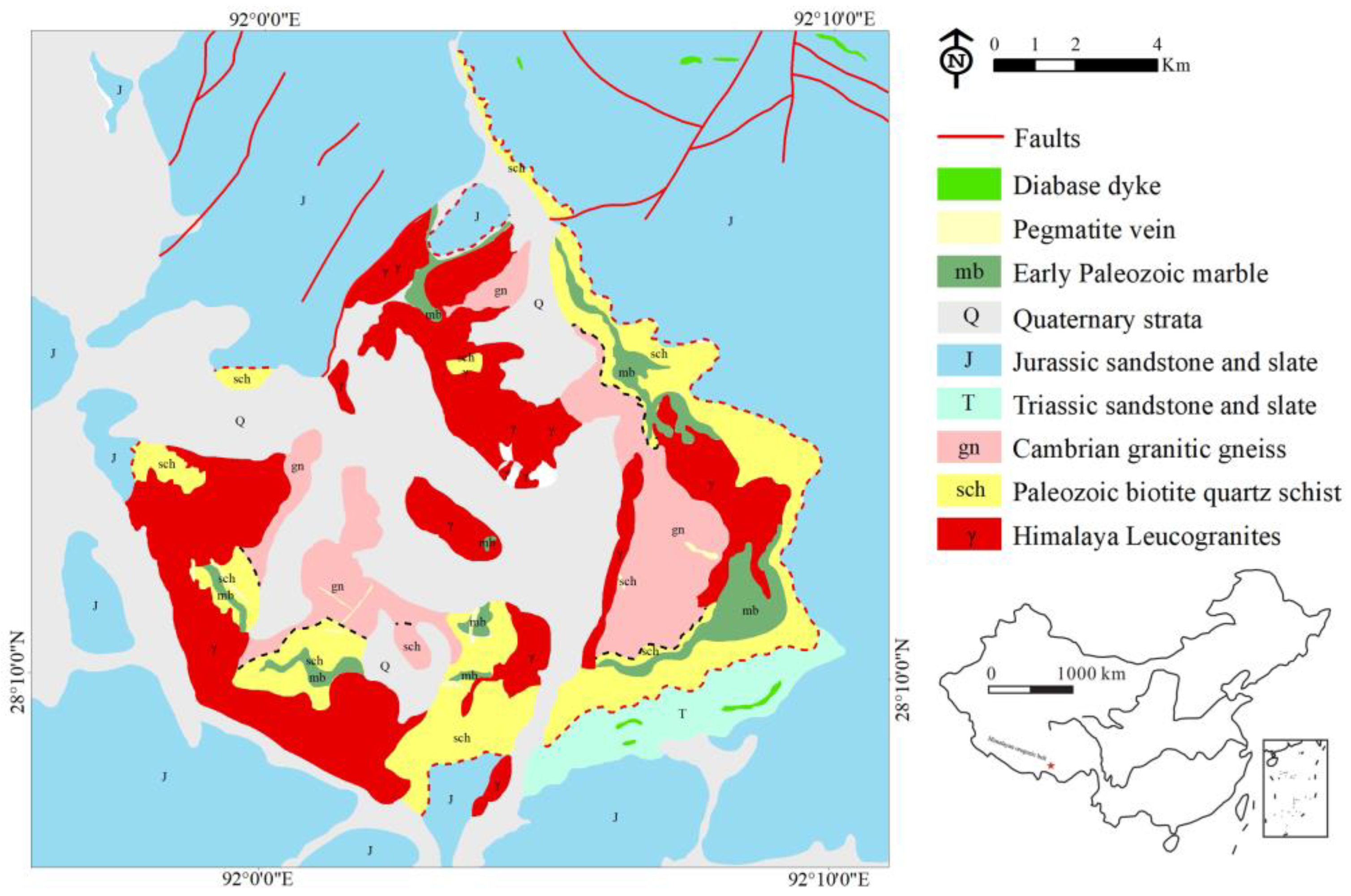
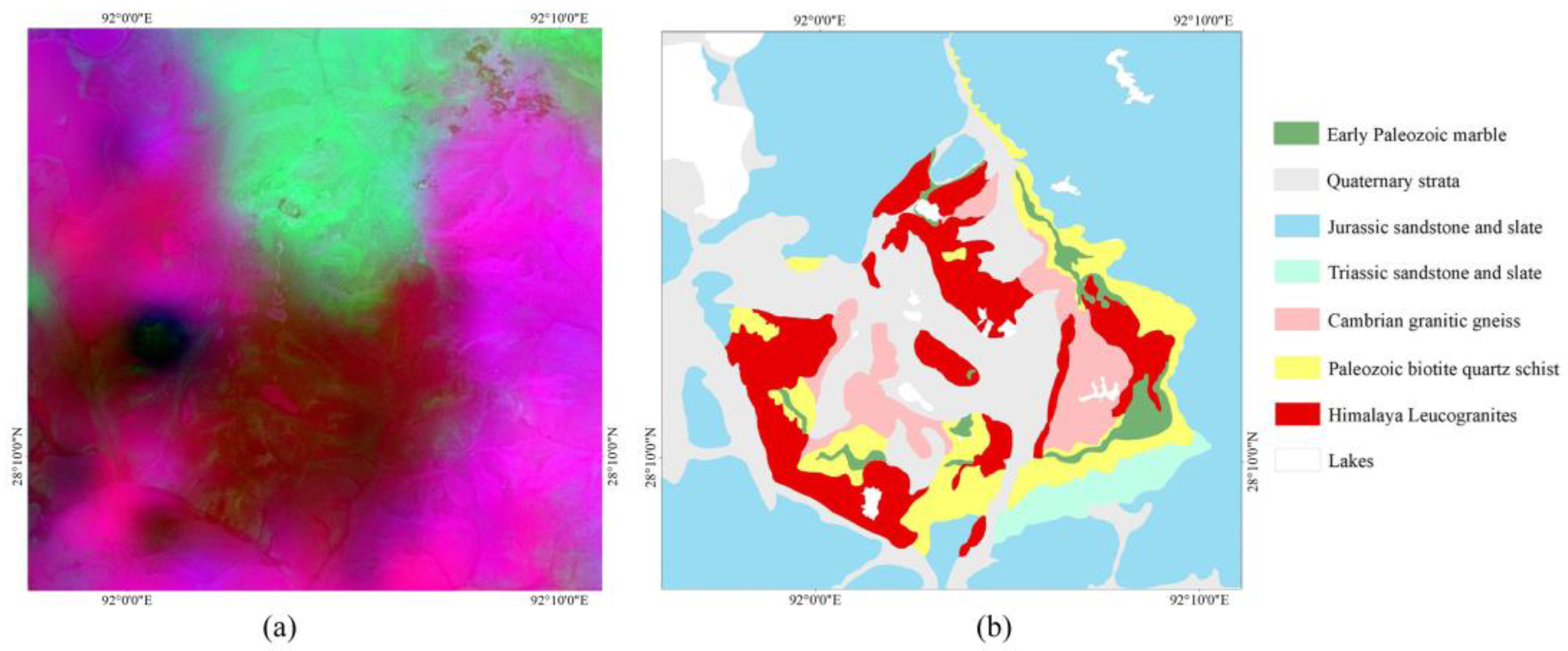
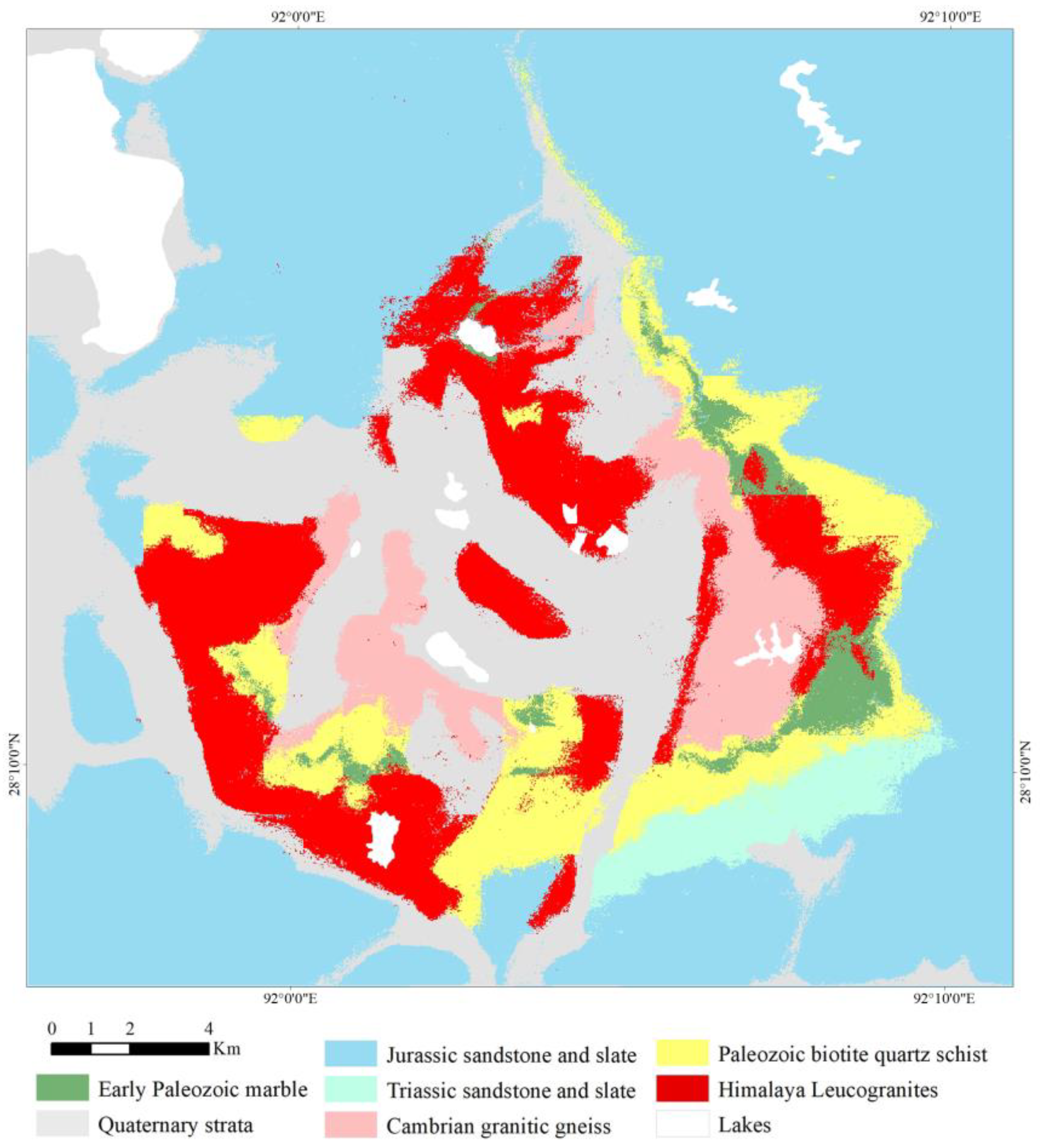
Seven lithologic units are exposed in the Cuonadong dome: Jurassic sandstone and slate, Early Paleozoic marble, Triassic sandstone and slate, Cambrian granitic gneiss, Paleozoic biotite quartz schist, Quaternary strata, and Himalayan leucogranites (Figure 3) [50,51]. Himalayan leucogranite is mainly composed of quartz (40%), plagioclase (25%), muscovite (15%), and potassium feldspar (10%), whereas the dominant minerals in the granitic gneiss surrounding with leucogranite are quartz (30%) and biotite (25%). The major element analysis reports higher SiO2 (≥72 wt. %), Al2O3 (≥14 wt. %), Na2O + K2O (≥8% wt.%), and lower CaO (≤2 wt. %), MgO (≤1 wt. %), and Fe2O3 (≤1 wt. %) [52,53,54]. Geophysical explorations revealed that the leucogranite belts are characterized by medium-higher magnetic susceptibility, lower density, lower gravity anomalies, and higher resistivity [55,56]. Such petrographic properties determine the specific chemical, physical, and spectral characteristics of these lithologic units, enabling them to be identified and distinguished through various geodata.
3.2. Data and Preprocessing
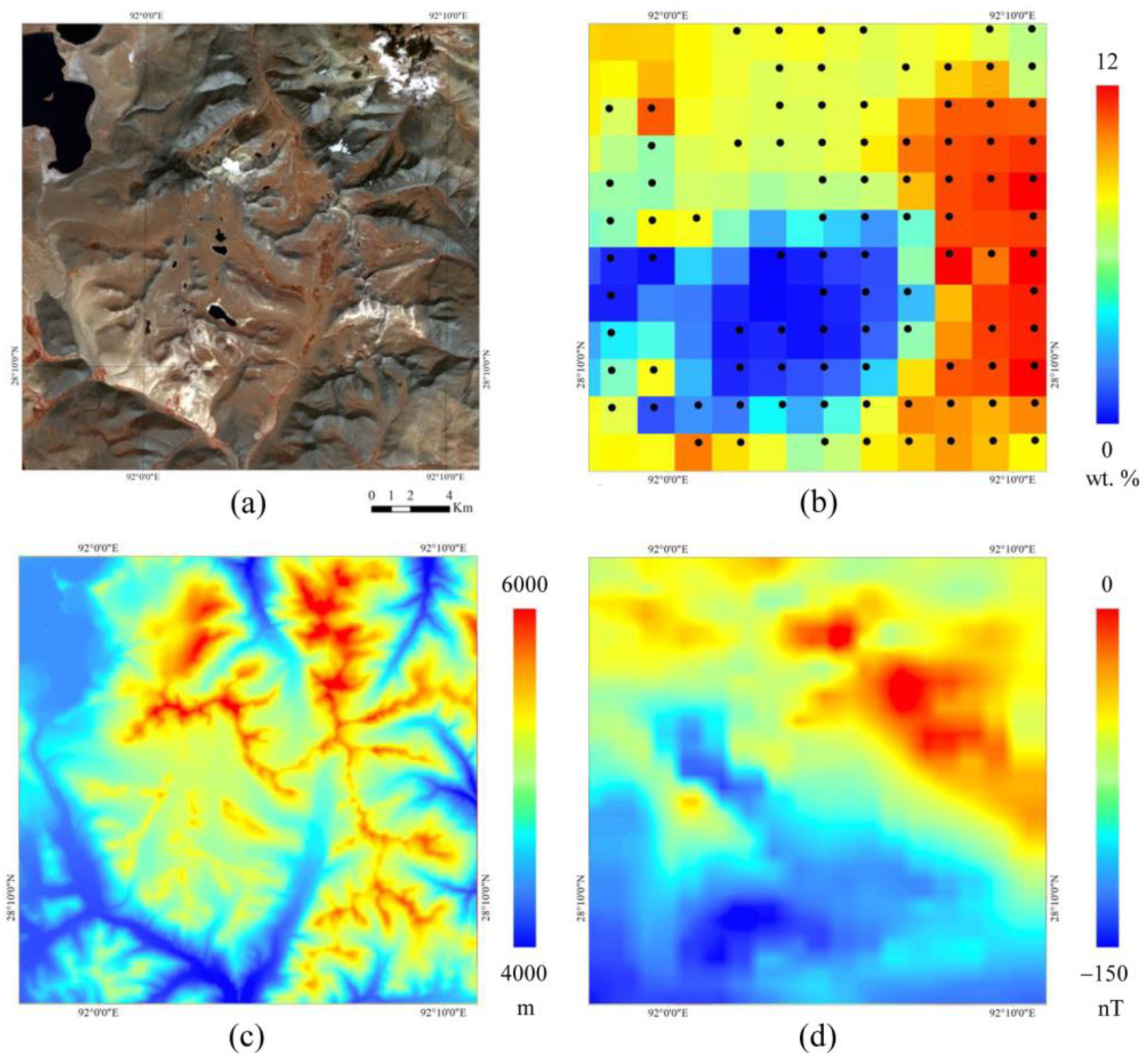
Four types of geodata were collected for lithologic mapping in the study area, including an ASTER remote sensing image that covers nine visible near infrared (VNIR) and short-wave infrared (SWIR) bands with spatial resolutions of 15 and 30 m, respectively (Figure 4a), geochemical exploration data at a scale of 1:200,000 with seven major oxides (SiO2, Al2O3, CaO, MgO, Fe2O3, Na2O, and K2O) (Figure 4b), high-precision PALSAR DEM data representing the topographic surface of geological features (Figure 4c), and aeromagnetic data at a scale of 1:200,000 (Figure 4d). The ASTER and PALSAR DEM images were captured on 17 February 2002 and 4 April 2018 in Level 1T, and were provided for free by the United States Geological Survey. The geochemical data were determined using X-ray fluorescence from the Chinese National Geochemical Mapping Project [57]. The aeromagnetic data from the airborne total magnetic intensity dataset were compiled by the China Geological Survey.
The preprocessing of ASTER remote sensing data includes radiation correction, atmospheric correction, and orthophoto correction. More specifically, the SWIR bands were first resampled to 15 m, consistent with the same resolution as the VNIR bands. Then, an ENVI’s FLAASH module was applied to remove the scattering and absorption effects from the atmosphere and correct image distortion caused by radiation errors. Orthophoto correction was also performed to eliminate the topography effect from topographic relief with the help of the RPC orthorectification module in ENVI. These corrections contribute to the identification accuracy of targets in mountainous areas. In addition, the aeromagnetic data are recommended to be filtered by magnetization conversion; the geochemical data should be transformed by the centered log-ratio transformations for addressing the closure effect of the compositional data [58,59]. The multi-source data fusion technology was then employed to fuse each element of the geochemical data (2 km) and aeromagnetic data (2 km) with nine VNIR-SWIR (15 m) bands in the ASTER images, according to the correlations between the spectral reflectance and geochemical element concentration or magnetic intensity. The fused image increases the spatial resolution of geochemical and aeromagnetic data from 2 km to 15 m, providing additional diagnostic information for lithological mapping. Figure 5 displays the fused nine-channel image (1611 × 1650 × 9 pixels) that merged ASTER, geochemical, aeromagnetic, and DEM data and the labeled geological map (1611 × 1650 pixels), containing seven lithologic units and an additional class covered with lakes and snow.
3.3. Building of Training Datasets
The input image was split into several part tiles of 256 × 256 × 9 pixels and fed into the FCN-8s model one by one. The training database was built using the sliding windows method at a stride size of 20 (Figure 1). A total of 1000 samples were collected by traversing the entire image and the geological map synchronously, occupying less than 1% of the total available patches. Each sample contained one or more labeled lithological classes. 80% of which were randomly selected as the training samples, and the remaining 20% were used to validate the model.
4. Results
4.1. Model Training
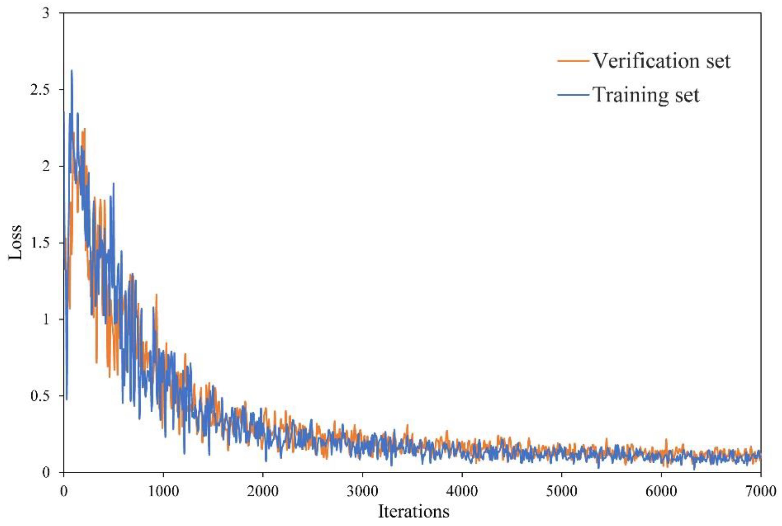
The hyperparameters of the FCN-8s model, including epoch, batch size, maximum iterations, and learning rate, were carefully optimized and set to 100, 5, 7000, and 0.0001, respectively. The stochastic gradient descent with momentum was selected as the dominant optimizer for solving the model optimization of weighting parameters [60]. The cross-entropy loss function continued to drop with the increasing iterative training times and finally reached a state of convergence, suggesting that the model was optimally tuned (Figure 6). Here, the loss is a summation of the errors made for each training pixel, indicating the performance of the model after each iteration of optimization [61]. It is worth mentioning that FCN enables the handling of unbalanced classes by weighting or sampling the loss [27].
4.2. Lithological Mapping
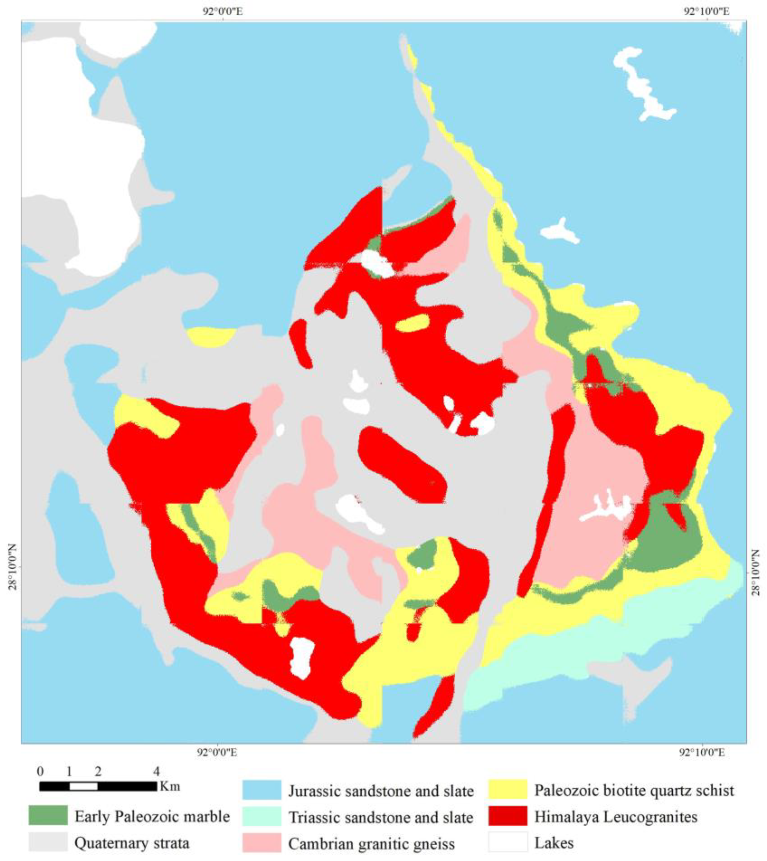
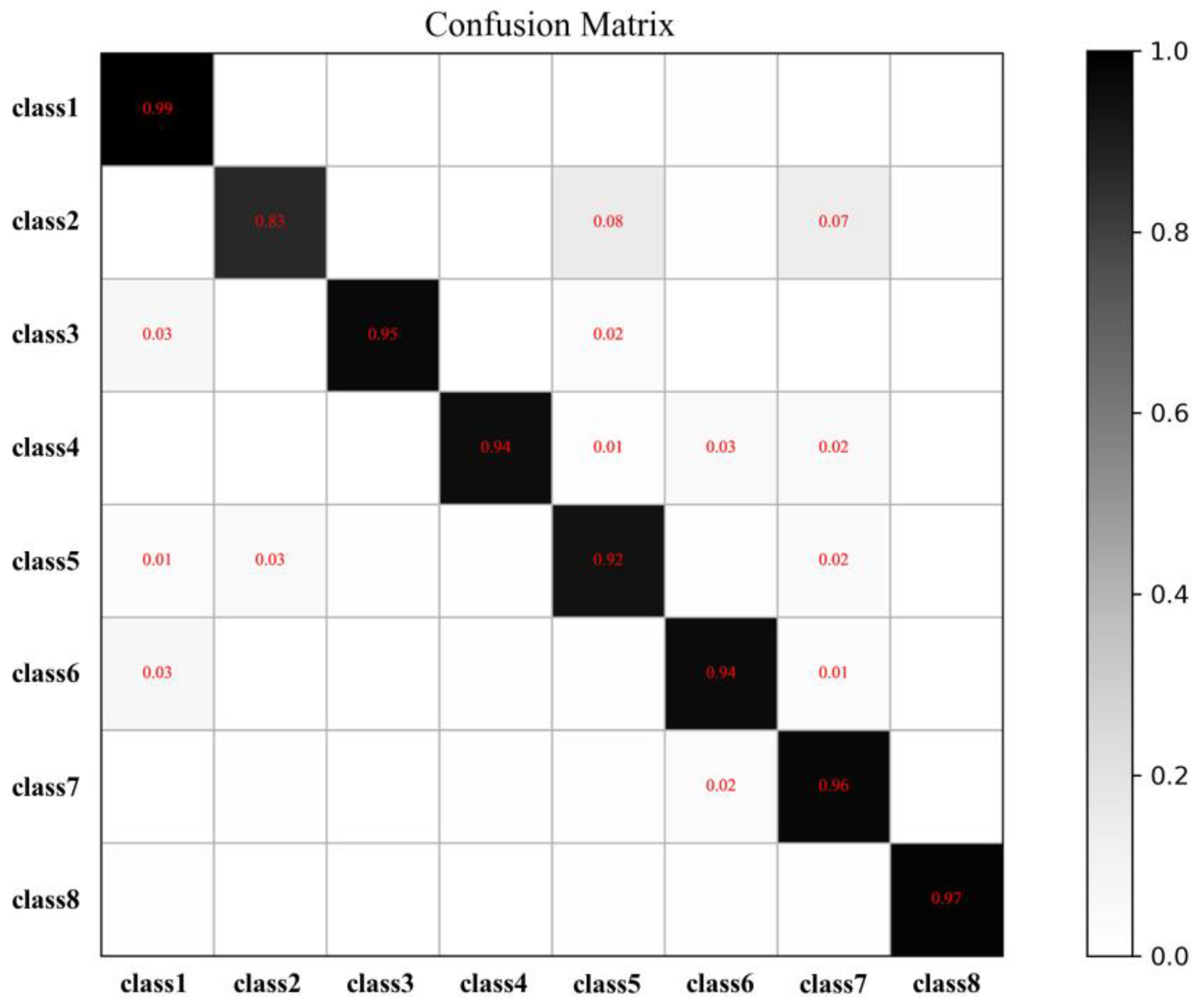
The fused nine-channel image was then fed into the trained model to predict the distribution of seven lithological classes, which was implemented with the help of the TensorFlow 1.2 platform in Python 3.6. Figure 7 presents the classification map obtained by the optimized FCN-8s model. From a visual point of view, almost all identified lithological units were consistent with the labeled geological map. From a quantitative point of view, the confusion matrix (Figure 8) showed that the model achieved excellent performance both in total accuracy (0.96) and the pixel accuracy for each class, as well as a high mIoU (0.9). Partial misclassifications were observed to exist at the edge and splice of different lithologic units. For example, strip-shaped early Paleozoic marbles were widely misclassified as Paleozoic biotite quartz schists, with pixel accuracies of 0.83 and 0.92, respectively. One possible reason is the difficulty associated with learning the correlations between the samples due to insufficient data caused by fewer outcropping areas; another reason is the highly similar mineral composition under strong skarnization, thus resulting in misclassification and omission. Splitting the input image into smaller parts is known to be a solution for solving these problems; however, such an operation expands the training set, which may increase the computational burden. Nevertheless, the above evidence demonstrates that the FCN-8s model has a capability to provide a solution for mapping geological target features by exploring the deeper hidden relationships among multi-source data. The integration of geochemical, geophysical, spatial, spectral, and topographic data in remote sensing images provides additional supplemental information from various perspectives and facilitates the discrimination of lithological units.
To further illustrate the effectiveness of the FCN-8s model in lithological mapping, a comparative study was implemented using the classic random forest algorithm with fused data. Random forest is a machine learning method that is built on multiple decision trees using the idea of ensemble learning [62]. Random forest is widely used in geological feature mapping, benefitting from its high classification accuracy and low bias [63,64]. The parameters of the random forest model—number of trees (ntree) and number of variables at each node (mtry)—were set to 200 and 3, respectively; the training set was built by selecting 10% of samples (pixels) randomly in each class, which is consistent with previous studies [5], for quantitative comparison.
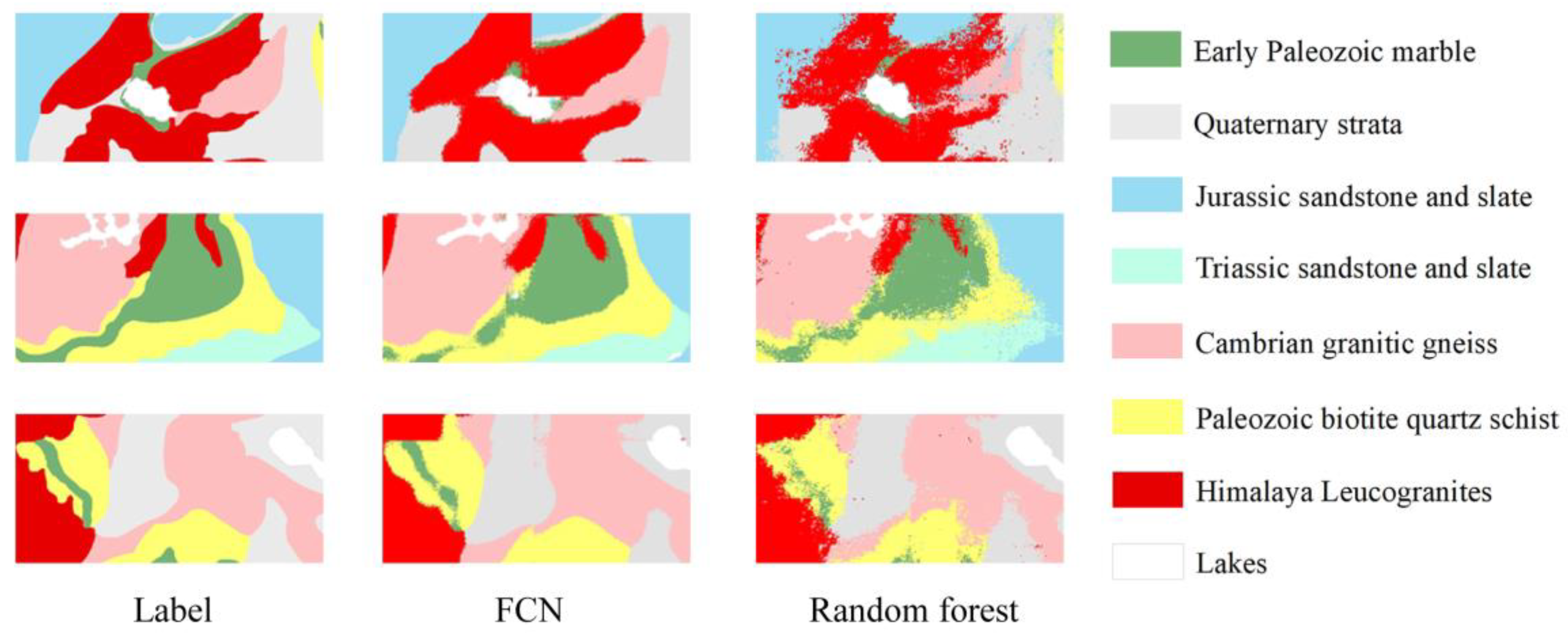
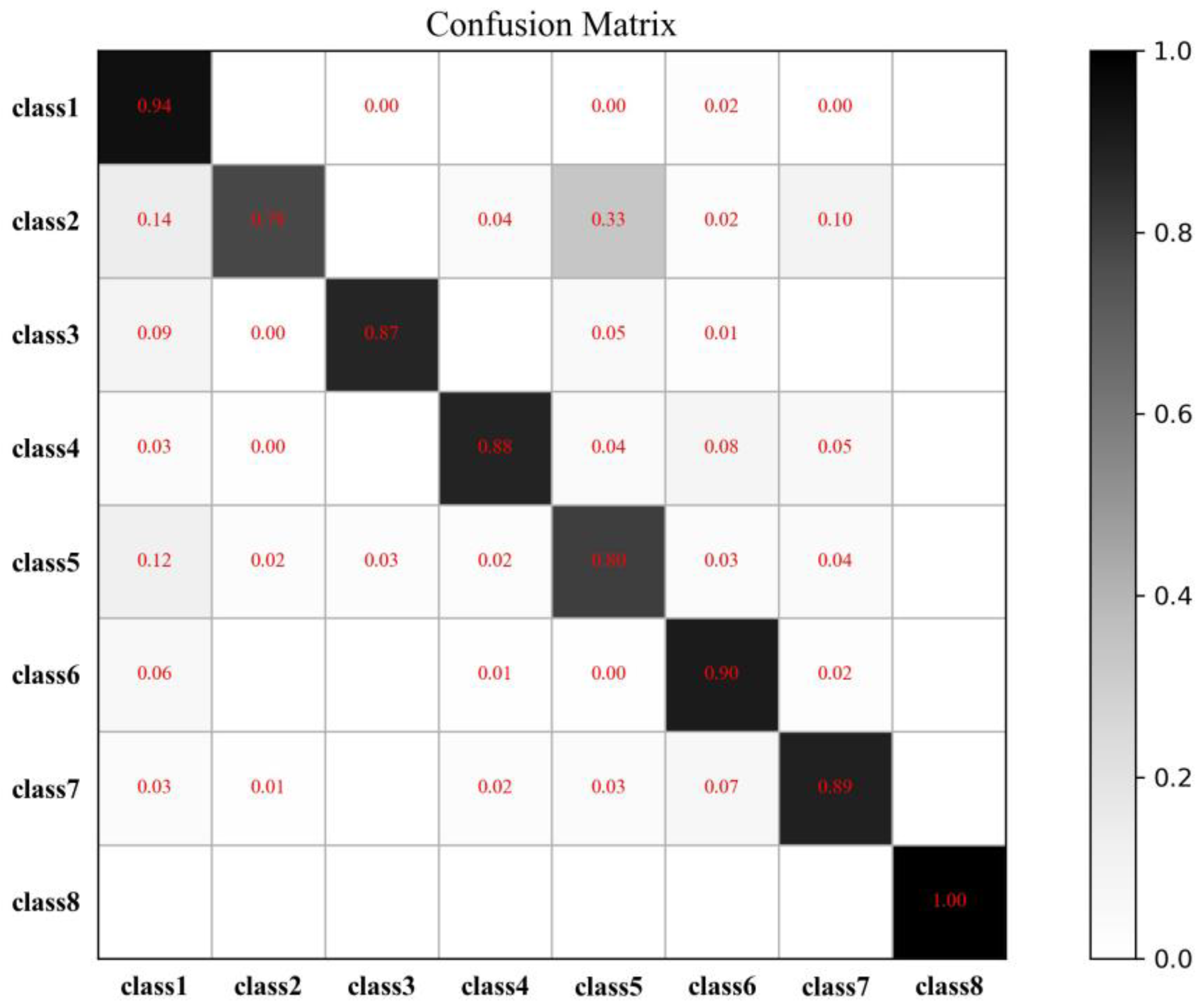
Figure 9 shows the pixel-wise classification map obtained using the random forest model with the fused data. Evidently, FCN-8s outperformed the random forest model with little “salt-and-pepper” noise and clear geological boundaries. Moreover, the FCN model restrained numerous misclassifications that occurred in the classification map delineated by random forest, such as the Paleozoic biotite quartz schist, early Paleozoic marble, and Himalayan leucogranites (Figure 10); this is because FCN can extract deeper semantic information per layers by convolution network and recover the size of feature maps by deconvolution operation, especially the details of the boundaries. Compared with the confusion matrix of random forest (Figure 11), the FCN-8s model improved the mean IoU from 0.85 to 0.90 and the total classification accuracy by more than 5%. For lithologic units with large coverage, such as Jurassic sandstone, slate and Quaternary strata, no significant improvements were observed, owing to the obvious differences in mineral composition that are easily discriminated. For those with minor coverage, such as Paleozoic marble and Triassic sandstone and slate, there was a noticeable improvement in classification accuracy of up to 8%. Nevertheless, quite a few Paleozoic biotite quartz schists were wrongly divided into early Paleozoic marbles by FCN-8s or the random forest model. On the one hand, these two lithologic units are mainly composed of carbonate minerals, which brings similar geochemical and spectral characteristics that are difficult to distinguish. On the other hand, the irregular distribution of lithological units decreases the size of the receptive field in the neural network, thus limiting the learning of lithological features and impeding the improvement of classification performance.
5. Discussion
Himalayan leucogranite has received increasing attention owing to its confirmed potential to host rare earth polymetallic mineral resources. Hence, how to map the spatial distribution of Himalayan leucogranites is considered as a primary task in exploring rare metal deposits. Fortunately, the distinctive geochemical, geophysical, and spectral properties are beneficial to the discrimination of Himalayan leucogranite. Previous studies have delineated both the large-scale and small-scale spatial distributions of leucogranites in the Himalayan orogenic belt [65] and Cuonadong dome [5,64], respectively, achieving a high identification accuracy of 0.84 by integrating geochemical and remote sensing images, with the support of random forest [5].
However, finding an approach to better identify geological features has always been a challenge. Lithology is formed under the joint action of a variety of geological features, which have spatially complex structural characteristics in geophysical, geochemical and remote sensing spectral information. The method mentioned above belongs to the shallow machine learning algorithm, which is powerless facing the complex nonlinear relationships and spatial patterns among multi-source data, and thus may restrict the rare metal exploration in this area. Accordingly, the results of this study improve the classification accuracy of leucogranites by 5% in the same study area after adding DEM topographic and aeromagnetic information. Remote sensing images provide more diagnostic bands and enrich the spatial details of geochemical and geophysical data; DEM data supplement the analysis of topographic characteristics related to weathering and erosion. The integration of the three types of geodata captures the complementary advantages of multi-source data. On this basis, this study introduced an FCN-8s model to promote the discrimination of highly similar lithological units, which can provide sufficient training samples and make it less expensive computationally than the patch-based approach; this is because no redundant operations and repeated calculations need to be performed on neighboring patches. The FCN-8s model further reaches considerable classification accuracy of up to 0.96 by learning the deep-level context correlation between multi-source data. The above descriptions prove the effectiveness of the proposed FCN-8s in mapping geological target features for mineral exploration.
6. Conclusions
This study introduces an accessible and robust way for geological feature mapping by incorporating deep learning algorithm and multi-source data fusion technology, aiming to improve the classification accuracy of lithological units. Multi-source data fusion technology was first employed to provide abundant diagnostic information. An FCN classification model was then built based on the well-known VGG-19 network to identify the distribution of geological features. This joint approach was illustrated by a case study in mapping seven lithological units in the Cuonadong dome, Tibet, China, where rare earth polymetallic deposits have been discovered. Three conclusions can be drawn based on the results:
- (1)
- The multi-source data fusion technology integrates ASTER remote sensing images, geochemical exploration data, PALSAR DEM data, and aeromagnetic data at various scales, providing a comprehensive analysis of geodata rather than a single type of data resource.
- (2)
- FCN is a specially designed semantic segmentation model that dominates in end-to-end and pixel-wise prediction with an arbitrary input size. FCN retains the advantages of feature extraction in CNN and solves the problem of classifying each pixel in an image through deconvolution operations and skip connections, making it an innovative alternative for lithological mapping.
- (3)
- A comparative study was carried out, proving that the proposed framework is effective and successful in geological feature mapping from the viewpoints of vision and quantification. The proposed FCN-8s model increased the classification accuracy of leucogranites by 9% compared to that reported in previous studies by extracting deeper-level hidden information from multi-source data.
Author Contributions
Conceptualization, Z.W. and R.Z.; writing—original draft preparation, Z.W. and R.Z.; software, Z.W. and H.L. All authors have read and agreed to the published version of the manuscript.
Funding
This research was jointly supported by the National Natural Science Foundation of China (No. 41972303, 42102332) and the Fundamental Research Funds for the Central Universities (No. 162301202684).
Institutional Review Board Statement
Not applicable.
Informed Consent Statement
Not applicable.
Data Availability Statement
Not applicable.
Acknowledgments
The authors would like to thank the editor and three anonymous reviewers for providing insightful and helpful comments.
Conflicts of Interest
The authors declare no conflict of interest.
References
- Harris, J.R.; Grunsky, E.C. Predictive lithological mapping of Canada’s North using Random Forest classification applied to geophysical and geochemical data. Comput. Geosci. 2015, 80, 9–25. [Google Scholar] [CrossRef]
- Othman, A.A.; Gloaguen, R. Integration of spectral, spatial and morphometric data into lithological mapping: A comparison of different Machine Learning Algorithms in the Kurdistan Region, NE Iraq. J. Asian Earth Sci. 2017, 146, 90–102. [Google Scholar] [CrossRef]
- Pal, M.; Rasmussen, T.; Porwal, A. Optimized lithological mapping from multispectral and hyperspectral remote sensing images using fused multi-classifiers. Remote Sens. 2020, 12, 177. [Google Scholar] [CrossRef] [Green Version]
- Shirmard, H.; Farahbakhsh, E.; Muller, D.; Chandra, R. A review of machine learning in processing remote sensing data for mineral exploration. arXiv 2021, arXiv:2103.07678. [Google Scholar] [CrossRef]
- Wang, Z.; Zuo, R.; Jing, L. Fusion of Geochemical and Remote-Sensing Data for Lithological Mapping Using Random Forest Metric Learning. Math. Geosci. 2021, 53, 1125–1145. [Google Scholar] [CrossRef]
- LeCun, Y.; Bengio, Y.; Hinton, G. Deep learning. Nature 2015, 521, 436–444. [Google Scholar] [CrossRef] [PubMed]
- Goodfellow, I.; Bengio, Y.; Courville, A. Deep Learning; MIT Press: Cambridge, MA, USA, 2016. [Google Scholar]
- Zuo, R.; Xiong, Y.; Wang, J.; Carranza, E.J.M. Deep learning and its application in geochemical mapping. Earth-Sci. Rev. 2019, 192, 1–14. [Google Scholar] [CrossRef]
- Reichstein, M.; Camps-Valls, G.; Stevens, B.; Jung, M.; Denzler, J.; Carvalhais, N. Deep learning and process understanding for data-driven Earth system science. Nature 2019, 566, 195–204. [Google Scholar] [CrossRef] [PubMed]
- Xiong, Y.; Zuo, R. Recognizing multivariate geochemical anomalies for mineral exploration by combining deep learning and one-class support vector machine. Comput. Geosci. 2020, 140, 104484. [Google Scholar] [CrossRef]
- Xiong, Y.; Zuo, R. Robust Feature Extraction for Geochemical Anomaly Recognition Using a Stacked Convolutional Denoising Autoencoder. Math. Geosci. 2021. [Google Scholar] [CrossRef]
- Li, T.; Zuo, R.; Xiong, Y.; Peng, Y. Random-drop data augmentation of deep convolutional neural network for mineral prospectivity mapping. Nat. Resour. Res. 2021, 30, 27–38. [Google Scholar] [CrossRef]
- Li, S.; Chen, J.; Liu, C.; Wang, Y. Mineral Prospectivity Prediction via Convolutional Neural Networks Based on Geological Big Data. J. Earth Sci. 2021, 32, 327–347. [Google Scholar] [CrossRef]
- Luo, Z.; Zuo, R.; Xiong, Y.; Wang, X. Detection of geochemical anomalies related to mineralization using the GANomaly network. Appl. Geochem. 2021, 131, 105043. [Google Scholar] [CrossRef]
- Deng, L.; Yu, D. Deep learning: Methods and applications. Found. Trends Signal Process. 2014, 7, 197–387. [Google Scholar] [CrossRef] [Green Version]
- Albawi, S.; Mohammed, T.A.; Al-Zawi, S. Understanding of a convolutional neural network. In Proceedings of the International Conference on Engineering and Technology (ICET), Antalya, Turkey, 21–23 August 2017; pp. 1–6. [Google Scholar] [CrossRef]
- Zhang, C.; Zuo, R.; Xiong, Y. Detection of the multivariate geochemical anomalies associated with mineralization using a deep convolutional neural network and a pixel-pair feature method. Appl. Geochem. 2021, 130, 104994. [Google Scholar] [CrossRef]
- Zhang, S.; Carranza, E.J.M.; Wei, H.; Xiao, K.; Yang, F.; Xiang, J.; Zhang, S.; Xu, Y. Data-driven mineral prospectivity mapping by joint application of unsupervised convolutional auto-encoder network and supervised convolutional neural network. Nat. Resour. Res. 2021, 30, 1011–1031. [Google Scholar] [CrossRef]
- Sherrah, J. Fully convolutional networks for dense semantic labelling of high-resolution aerial imagery. arXiv 2016, arXiv:1606.02585. [Google Scholar]
- Zuo, R. Geodata science-based mineral prospectivity mapping: A review. Nat. Resour. Res. 2020, 29, 3415–3424. [Google Scholar] [CrossRef]
- Zuo, R.; Xiong, Y. Geodata science and geochemical mapping. J. Geochem. Explor. 2020, 209, 106431. [Google Scholar] [CrossRef]
- Ge, W.; Cheng, Q.; Tang, Y.; Jing, L.; Gao, C. Lithological classification using sentinel-2A data in the Shibanjing ophiolite complex in inner Mongolia, China. Remote Sens. 2018, 10, 638. [Google Scholar] [CrossRef] [Green Version]
- Brandmeier, M.; Chen, Y. Lithological classification using multi-sensor data and convolutional neural networks. ISPRS-Int. Arch. Photogramm. Remote Sens. Spat. Inf. Sci. 2019, 42, 55–59. [Google Scholar] [CrossRef] [Green Version]
- Ghamisi, P.; Rasti, B.; Yokoya, N.; Wang, Q.; Hofle, B.; Bruzzone, L.; Bovolo, F.; Chi, M.; Anders, K.; Gloaguen, R.; et al. Multisource and multitemporal data fusion in remote sensing: A comprehensive review of the state of the art. IEEE Geosci. Remote Sens. Mag. 2019, 7, 6–39. [Google Scholar] [CrossRef] [Green Version]
- Thiele, S.T.; Lorenz, S.; Kirsch, M.; Acosta, I.C.C.; Tusa, L.; Herrmann, E.; Möckel, R.; Gloaguen, R. Multi-scale, multi-sensor data integration for automated 3-D geological mapping. Ore Geol. Rev. 2021, 136, 104252. [Google Scholar] [CrossRef]
- Long, J.; Shelhamer, E.; Darrell, T. Fully convolutional networks for semantic segmentation. In Proceedings of the IEEE Conference on Computer Vision and Pattern Recognition, Boston, MA, USA, 7–12 June 2015; pp. 3431–3440. [Google Scholar] [CrossRef] [Green Version]
- Shelhamer, E.; Long, J.; Darrell, T. Fully convolutional neural networks for semantic segmentation. arXiv 2016, arXiv:1605.06211. [Google Scholar]
- Fu, G.; Liu, C.; Zhou, R.; Sun, T.; Zhang, Q. Classification for high resolution remote sensing imagery using a fully convolutional network. Remote Sens. 2017, 9, 498. [Google Scholar] [CrossRef] [Green Version]
- Zou, L.; Zhu, X.; Wu, C.; Liu, Y.; Qu, L. Spectral–spatial exploration for hyperspectral image classification via the fusion of fully convolutional networks. IEEE J. Sel. Top. Appl. Earth Obs. Remote Sens. 2020, 13, 659–674. [Google Scholar] [CrossRef]
- Wang, J.; Song, L.; Li, Z.; Sun, H.; Sun, J.; Zheng, N. End-to-end object detection with fully convolutional network. In Proceedings of the IEEE/CVF Conference on Computer Vision and Pattern Recognition, Virtual, 20–25 June 2021; pp. 15849–15858. [Google Scholar]
- Ding, H.; Jing, L.; Li, H.; Tang, Y.; Ma, H.; Zhu, B.; Wang, W.; Qiu, L. A method and system for improving the resolution of geochemical layers. Chinese Patents No. 201811275285.4, 28 August 2020. [Google Scholar]
- Maggiori, E.; Tarabalka, Y.; Charpiat, G.; Alliez, P. Fully convolutional neural networks for remote sensing image classification. In Proceedings of the IEEE International Geoscience and Remote Sensing Symposium (IGARSS), Beijing, China, 10–15 July 2016; pp. 5071–5074. [Google Scholar] [CrossRef] [Green Version]
- He, C.; He, B.; Tu, M.; Wang, Y.; Qu, T.; Wang, D.; Liao, M. Fully convolutional networks and a manifold graph embedding-based algorithm for polsar image classification. Remote Sens. 2020, 12, 1467. [Google Scholar] [CrossRef]
- Simonyan, K.; Zisserman, A. Very deep convolutional networks for large-scale image recognition. arXiv 2014, arXiv:1409.1556. [Google Scholar]
- Noh, H.; Hong, S.; Han, B. Learning deconvolution network for semantic segmentation. In Proceedings of the IEEE International Conference on Computer Vision, Santiago, Chile, 13–16 December 2015; pp. 1520–1528. [Google Scholar] [CrossRef] [Green Version]
- Zhang, J.; Pan, J.; Lai, W.; Lau, R.W.; Yang, M. Learning fully convolutional networks for iterative non-blind deconvolution. In Proceedings of the IEEE Conference on Computer Vision and Pattern Recognition, Honolulu, HI, USA, 21–26 July 2017; pp. 3817–3825. [Google Scholar] [CrossRef] [Green Version]
- Sokolova, M.; Japkowicz, N.; Szpakowicz, S. Beyond accuracy, F-score and ROC: A family of discriminant measures for performance evaluation. In Proceedings of the Australasian Joint Conference on Artificial Intelligence, Hobart, TAS, Australia, 4–8 December 2006; Springer: Berlin/Heidelberg, Germany; pp. 1015–1021. [Google Scholar] [CrossRef] [Green Version]
- Sokolova, M.; Lapalme, G. A systematic analysis of performance measures for classification tasks. Inf. Process. Manag. 2009, 45, 427–437. [Google Scholar] [CrossRef]
- Rahman, M.A.; Wang, Y. Optimizing intersection-over-union in deep neural networks for image segmentation. In Proceedings of the International Symposium on Visual Computing, Las Vegas, NV, USA, 12–14 December 2006; Springer: Cham, Germany, 10 December 2016; pp. 234–244. [Google Scholar] [CrossRef]
- Rezatofighi, H.; Tsoi, N.; Gwak, J.; Sadeghian, A.; Reid, I.; Savarese, S. Generalized intersection over union: A metric and a loss for bounding box regression. In Proceedings of the IEEE/CVF Conference on Computer Vision and Pattern Recognition, Long Beach, CA, USA, 15–20 June 2019; pp. 658–666. [Google Scholar] [CrossRef] [Green Version]
- Wu, F.; Liu, Z.; Liu, X.; Ji, W. Himalayan leucogranite: Petrogenesis and implications to orogenesis and plateau uplift. Acta Petrol. Sin. 2015, 31, 1–36. [Google Scholar]
- Wu, F.; Liu, X.; Ji, W.; Wang, J.; Yang, L. Highly fractionated granites: Recognition and research. Sci. China Earth Sci. 2017, 60, 1201–1219. [Google Scholar] [CrossRef]
- Wang, R.; Wu, F.; Xie, L.; Liu, X.; Wang, J.; Yang, L.; Lai, W.; Liu, C. A preliminary study of rare-metal mineralization in the Himalayan leucogranite belts, South Tibet. Sci. China Earth Sci. 2017, 60, 1655–1663. [Google Scholar] [CrossRef]
- Xie, L.; Tao, X.; Wang, R.; Wu, F.; Liu, C.; Liu, X.; Li, X.; Zhang, R. Highly fractionated leucogranites in the eastern Himalayan Cuonadong dome and related magmatic Be–Nb–Ta and hydrothermal Be–W–Sn mineralization. Lithos 2020, 354, 105286. [Google Scholar] [CrossRef]
- Wu, F.; Liu, X.; Liu, Z.; Wang, R.; Xie, L.; Wang, J.; Ji, W.; Yang, L.; Liu, C.; Khanal, G.P. Highly fractionated Himalayan leucogranites and associated rare-metal mineralization. Lithos 2020, 352, 105319. [Google Scholar] [CrossRef]
- Cao, H.; Li, G.; Zhang, Z.; Zhang, L.; Dong, S.; Xia, X.; Liang, W.; Fu, J.; Huang, Y.; Xiang, A. Miocene Sn polymetallic mineralization in the Tethyan Himalaya, southeastern Tibet: A case study of the Cuonadong deposit. Ore Geol. Rev. 2020, 119, 103403. [Google Scholar] [CrossRef]
- Xiang, A.; Li, W.; Li, G.; Dai, Z.; Yu, H.; Yang, F. Mineralogy, isotope geochemistry and ore genesis of the miocene Cuonadong leucogranite-related Be-W-Sn skarn deposit in Southern Tibet. J. Asian Earth Sci. 2020, 196, 104358. [Google Scholar] [CrossRef]
- Fu, J.; Li, G.; Wang, G.; Zhang, L.; Liang, W.; Zhang, X.; Jiao, Y.; Huang, Y. Structural and thermochronologic constraints on skarn rare-metal mineralization in the Cenozoic Cuonadong Dome, Southern Tibet. J. Asian Earth Sci. 2021, 205, 104612. [Google Scholar] [CrossRef]
- Li, G.; Zhang, L.; Jiao, Y.; Xia, X.; Dong, S.; Fu, J.; Liang, W.; Zhang, Z.; Wu, J.; Dong, L. First discovery and implications of Cuonadong superlarge Be-W-Sn polymetallic deposit in Himalayan metallogenic belt, southern Tibet. Miner. Depos. 2017, 36, 1003–1008. [Google Scholar]
- Liang, W.; Li, G.; Zhang, L.; Fu, J.; Zhang, Z. Cuonadong Be-rare polymetallic metal deposit: Constraints from Ar-Ar age of hydrothermal muscovite. Sediment. Geol. Tethyan Geol. 2020, 40, 76–81. [Google Scholar]
- Cao, H.; Li, G.; Zhang, R.; Zhang, Y.; Zhang, L.; Dai, Z.; Zhang, Z.; Liang, W.; Dong, S.; Xia, X. Genesis of the Cuonadong tin polymetallic deposit in the Tethyan Himalaya: Evidence from geology, geochronology, fluid inclusions and multiple isotopes. Gondwana Res. 2021, 92, 72–101. [Google Scholar] [CrossRef]
- Xie, J.; Qiu, H.; Bai, X.; Zhang, W.; Wang, Q.; Xia, X. Geochronological and geochemical constraints on the Cuonadong leucogranite, eastern Himalaya. Acta Geochim. 2018, 37, 347–359. [Google Scholar] [CrossRef]
- Xia, X.; Li, G.; Cao, H.; Liang, W.; Fu, J. Petrogenic Age and Geochemical Characteristics of the Mother Rock of Skarn Type Ore Body in the Cuonadong Be-W-Sn Polymetallic Deposit, Southern Tibet. Earth Sci. 2019, 44, 2207–2223. [Google Scholar]
- Huang, Y.; Fu, J.; Li, G.; Zhang, L.; Liu, H. Determination of Lalong Dome in South Tibet and New Discovery of Rare Metal Mineralization. Earth Sci. 2019, 44, 2197–2206. [Google Scholar]
- Jiao, Y.; Huang, X.; Li, G.; Liang, S.; Guo, J. Deep Structure and Mineralization of Zhaxikang Ore-Concentration Area, South Tibet: Evidence from Geophysics. Earth Sci. 2019, 44, 2117–2128. [Google Scholar]
- Jiao, Y.; Huang, X.; Liang, S.; Zhang, Z.; Li, G. Deep structure and prospecting significance of the Cuonadong dome, Tethys Himalaya, China: Geophysical constraints. Geol. J. 2021, 56, 253–264. [Google Scholar] [CrossRef]
- Xie, X.; Mu, X.; Ren, T. Geochemical mapping in China. J. Geochem. Explor. 1997, 60, 99–113. [Google Scholar]
- Aitchison, J. The statistical analysis of compositional data. J. R. Stat. Soc. Ser. B (Methodol.) 1982, 44, 139–160. [Google Scholar] [CrossRef]
- Zuo, R.; Xia, Q.; Wang, H. Compositional data analysis in the study of integrated geochemical anomalies associated with mineralization. Appl. Geochem. 2013, 28, 202–211. [Google Scholar] [CrossRef]
- Sutskever, I.; Martens, J.; Dahl, G.; Hinton, G. On the importance of initialization and momentum in deep learning. In Proceedings of the International Conference on Machine Learning, Atlanta, GA, USA, 16–21 June 2013; pp. 1139–1147. [Google Scholar]
- Murphy, K.P. Machine Learning: A Probabilistic Perspective; MIT Press: Cambridge, MA, USA, 2012. [Google Scholar]
- Breiman, L. Random forests. Mach. Learn. 2001, 45, 5–32. [Google Scholar] [CrossRef] [Green Version]
- Parsa, M.; Maghsoudi, A.; Yousefi, M. Spatial analyses of exploration evidence data to model skarn-type copper prospectivity in the Varzaghan district, NW Iran. Ore Geol. Rev. 2018, 92, 97–112. [Google Scholar] [CrossRef]
- Wang, Z.; Zuo, R.; Dong, Y. Mapping of himalaya leucogranites based on ASTER and sentinel-2A datasets using a hybrid method of metric learning and random forest. IEEE J. Sel. Top. Appl. Earth Obs. Remote Sens. 2020, 13, 1925–1936. [Google Scholar] [CrossRef]
- Wang, Z.; Zuo, R.; Dong, Y. Mapping Himalayan leucogranites using a hybrid method of metric learning and support vector machine. Comput. Geosci. 2020, 138, 104455. [Google Scholar] [CrossRef]
Figure 1.
A brief overview of the proposed framework. Multi-source data fusion technology was first adopted to integrate remote sensing images, geochemical exploration data, and aeromagnetic data at various scales. An FCN model was then applied to learn the global, local, and contextual features of the fused geodata for lithological mapping. The training and validation databases were built using the sliding windows method based on a labeled geological map.

Figure 2.
FCN architecture design. The model was constructed from the VGG-19 network [34], where the first part is a convolution network similar to a CNN, and the second part is a deconvolution network with skip connection. The final output is obtained by a continuous upsampling operation and connecting with the corresponding pooled map.

Figure 3.
Simplified geological map of the Cuonadong Dome, Tibet, China, containing seven lithologic units (modified from [49]).
Figure 3.
Simplified geological map of the Cuonadong Dome, Tibet, China, containing seven lithologic units (modified from [49]).

Figure 4.
Four types of geodata: (a) false-color composites of ASTER image (bands 3, 2, and 1) with a spatial resolution of 15 m, provided by the United States Geological Survey; (b) geochemical samples and concentration distribution at a scale of 1:200,000 (taking Fe2O3 as an example), provided by the Chinese National Geochemical Mapping Project; (c) high-precision PALSAR DEM data with a spatial resolution of 12.5 m, provided by the United States Geological Survey; and (d) aeromagnetic data at a scale of 1:200,000, provided by the China Geological Survey.

Figure 5.
Maps showing (a) the fused multi-resource data of four types of geodata, increasing the spatial resolution of geochemical and aeromagnetic data from 2 km to 15 m and (b) labeled image containing seven lithologic units based on the geological map.
Figure 5.
Maps showing (a) the fused multi-resource data of four types of geodata, increasing the spatial resolution of geochemical and aeromagnetic data from 2 km to 15 m and (b) labeled image containing seven lithologic units based on the geological map.

Figure 6.
Plot of loss function versus number of iterations for training and verification sets, indicating that the model was optimally tuned.
Figure 6.
Plot of loss function versus number of iterations for training and verification sets, indicating that the model was optimally tuned.

Figure 7.
Classification map obtained by the FCN-8s model and fused data, indicating that almost all identified lithological units were visually consistent with the labeled geological map.
Figure 7.
Classification map obtained by the FCN-8s model and fused data, indicating that almost all identified lithological units were visually consistent with the labeled geological map.

Figure 8.
Confusion matrix of the classification map obtained by the FCN-8s model and fused data. class1: Jurassic sandstone and slate; class2: Early Paleozoic marble; class3: Triassic sandstone and slate; class4: Cambrian granitic gneiss; class5: Paleozoic biotite quartz schist; class6: Quaternary strata; class7: Himalaya Leucogranites; class8: lakes.

Figure 9.
Classification map obtained by random forest model and fused data. The result show obvious “salt-and-pepper” noise.
Figure 9.
Classification map obtained by random forest model and fused data. The result show obvious “salt-and-pepper” noise.

Figure 10.
Magnified boundaries of lithological units. It is evident that FCN-8s outperformed the random forest model with clear geological boundaries and few misclassifications.
Figure 10.
Magnified boundaries of lithological units. It is evident that FCN-8s outperformed the random forest model with clear geological boundaries and few misclassifications.

Figure 11.
Confusion matrix of the classification obtained by the random forest model and fused data. class1: Jurassic sandstone and slate; class2: Early Paleozoic marble; class3: Triassic sandstone and slate; class4: Cambrian granitic gneiss; class5: Paleozoic biotite quartz schist; class6: Quaternary strata; class7: Himalaya Leucogranites; class8: lakes.


Table 1.
Parameters setting of FCN-8s model.
| Layer Name | Number | Filter Size | Feature Dimensions |
|---|---|---|---|
| Input | 256 × 256 × 1 | ||
| Conv1 | 2 | 3 × 3 | 256 × 256 × 64 |
| Pool1 | 1 | 2 × 2 | 128 × 128 × 64 |
| Conv2 | 2 | 3 × 3 | 128 × 128 × 128 |
| Pool2 | 1 | 2 × 2 | 64 × 64 × 128 |
| Conv3 | 4 | 3 × 3 | 64 × 64 × 256 |
| Pool3 | 1 | 2 × 2 | 32 × 32 × 256 |
| Conv4 | 4 | 3 × 3 | 32 × 32 × 512 |
| Pool4 | 1 | 2 × 2 | 16 × 16 × 512 |
| Conv5 | 4 | 3 × 3 | 16 × 16 × 512 |
| Pool5 | 1 | 2 × 2 | 8 × 8 × 512 |
| Conv6 | 1 | 1 × 1 | 8 ×8 × 4096 |
| Dropout | 8 ×8 × 4096 | ||
| Conv7 | 1 | 1 × 1 | 8 ×8 × 4096 |
| Conv8 | 1 | 1 × 1 | 8 × 8 × 4096 |
| tConv1 | 1 | 2 × 2 | 16 × 16 × 512 |
| tConv2 | 1 | 2 × 2 | 32 × 32 × 256 |
| tConv3 | 1 | 8 × 8 | 256 × 256 × 2 |
| Softmax | |||
| Output | 256 × 256 × 1 |
Conv: convolution layer; Pool: max-pooling layer; tConv: deconvolution layer.
Publisher’s Note: MDPI stays neutral with regard to jurisdictional claims in published maps and institutional affiliations. |
© 2021 by the authors. Licensee MDPI, Basel, Switzerland. This article is an open access article distributed under the terms and conditions of the Creative Commons Attribution (CC BY) license (https://creativecommons.org/licenses/by/4.0/).
Share and Cite
MDPI and ACS Style
Wang, Z.; Zuo, R.; Liu, H. Lithological Mapping Based on Fully Convolutional Network and Multi-Source Geological Data. Remote Sens. 2021, 13, 4860. https://0-doi-org.brum.beds.ac.uk/10.3390/rs13234860
AMA Style
Wang Z, Zuo R, Liu H. Lithological Mapping Based on Fully Convolutional Network and Multi-Source Geological Data. Remote Sensing. 2021; 13(23):4860. https://0-doi-org.brum.beds.ac.uk/10.3390/rs13234860
Chicago/Turabian StyleWang, Ziye, Renguang Zuo, and Hao Liu. 2021. "Lithological Mapping Based on Fully Convolutional Network and Multi-Source Geological Data" Remote Sensing 13, no. 23: 4860. https://0-doi-org.brum.beds.ac.uk/10.3390/rs13234860
Note that from the first issue of 2016, this journal uses article numbers instead of page numbers. See further details here.