HF-Induced Modifications of the Electron Density Profile in the Earth’s Ionosphere Using the Pump Frequencies near the Fourth Electron Gyroharmonic

Abstract

We discuss results on plasma density profile modifications in the F-region ionosphere that are caused by HF heating with the frequency f₀ in the range [(−150 kHz)–(+75 kHz)] around the fourth electron gyroharmonic 4f_c. The experiments were conducted at the HAARP facility in June 2014. A multi-frequency Doppler sounder (MDS), which measures the phase and amplitude of reflected sounding radio waves, complemented by the observations of the stimulated electromagnetic emission (SEE) were used for the diagnostics of the plasma perturbations. We detected noticeable plasma expulsion from the reflection region of the pumping wave and from the upper hybrid region, where the expulsion from the latter was strongly suppressed for f₀ ≈ 4f_c. The plasma expulsion from the upper hybrid region was accompanied by the sounding wave’s anomalous absorption (AA) slower development for f₀ ≈ 4f_c. Furthermore, slower development and weaker expulsion were detected for the height region between the pump wave reflection and upper hybrid altitudes. The combined MDS and SEE allowed for establishing an interconnection between different manifestations of the HF-induced ionospheric turbulence and determining the altitude of the most effective pump wave energy input to ionospheric plasma by using the dependence on the offset between f₀ and 4f_c.

1. Introduction

A powerful O-mode electromagnetic pump wave transmitted from the ground into the bottom-site ionospheric F-region excites a wide range of plasma processes, leading to the appearance of artificial ionospheric turbulence (AIT), i.e., the generation of different HF and LF plasma modes; plasma density inhomogeneities of scales from tens of centimeters to kilometers; and causes electron heating, electron acceleration, ionization, generation of ionospheric airglow, etc. [1,2,3]. Diverse diagnostic methods and tools are used for studying the AIT, particularly, the sounding of the heated volume of the ionosphere using diagnostic waves and the registration of secondary, or stimulated, emission (SEE) in different frequency ranges.

The pump–plasma interaction is known to be the strongest near the pump wave (PW) reflection height z_r0 at which f_p(z_r0) equals the pump frequency f₀, and near the upper hybrid (UH) resonance height z_UH0, where f_p(z_UH0) = (f₀² − f_c²)^1/2 (here $f_{\mathrm{p}}=\left(1/2\pi \right){\left(e^{2}N/m{\epsilon }_0\right)}^{1/2}$ and f_c = eB/2πm are the electron plasma frequency and the electron cyclotron frequency, respectively; e and m are the electron charge and mass; N is the electron density; ${\epsilon }_0$the permittivity of free space; and B is the geomagnetic field strength). This corresponds to existing theoretical concepts and is confirmed by investigations of the HF-pumped ionospheric volume using multifrequency Doppler sounding (MDS) at the “Sura” and EISCAT heating facilities [4,5,6,7], which had revealed plasma expulsion from the resonance regions. During early MDS experiments, few low-power O-mode waves with frequencies f_i, i = 1, 2, …, k, around f₀ were used to probe different parts of the ionospheric plasma in or near the interaction regions. Measurements of time variations of probe wave phases allowed for measurement of the density profile modifications. In experiments, only a small number of frequencies of probing (diagnostic) waves could be used, i.e., $k\le 8,$ and the distance between neighbor “probing altitudes” in the ionosphere was typically 0.5–1 km. In [8], a way of increasing the number of diagnostic wave frequencies without adding transmitter(s) and, therefore, of decreasing the height step between neighbor probing altitudes was suggested (for details see Section 2). This method was successfully used in the MDS experiments at the “Sura” facility [9].

The HF pump-induced phenomena that occur in the resonance region depend noticeably on the proximity of the PW frequency f₀ to the electron cyclotron harmonics nf_c (n = 2, …, 7). This concerns the SEE, the cross-section of the aspect angle scattering, the anomalous absorption (AA) of the diagnostic waves with frequencies f_i close to f₀, the artificial airglow, the generation of artificial ionization layers, etc. An extensive literature is devoted to studying the dependences of these phenomena on $f_0-n{f}_{\mathrm{c}}$ [10,11,12,13,14,15,16,17,18,19,20,21,22,23,24,25,26,27,28,29,30].

SEE with frequencies f_SEE close to the pump wave frequency f₀ occurs due to the conversion of HF pump-driven electrostatic plasma modes, most notably Langmuir (L) and upper hybrid (UH) waves, into electromagnetic waves that are weaker than the reflected PW by 50–90 dB [10,31,32] and provide rich information about the AIT, thereby helping to identify nonlinear processes in the HF-pumped volume. The prominent SEE spectral features have long been used as indicators of specific nonlinear mode interactions in the altitude region between the reflection z_r0 of the O-mode pump and slightly below the upper hybrid resonance z_UH0. Several prominent SEE spectral features were established from numerous studies of stationary and dynamic SEE spectra that were performed at the European Incoherent Scatter (EISCAT), “Sura”, High-Frequency Active Auroral Research Program (HAARP), Arecibo and Space Plasma Exploration by Active Radar (SPEAR) heating facilities for 2.8 < f₀ < 10 MHz [8,9]. SEE spectral characteristics depend on the Δf_c = f₀ − nf_c offset of the PW frequency f₀ from the multiple electron gyroresonance nf_c. The most dramatic changes occur during the transition of f₀ via nf_c (e.g., from f₀ < nf_c to f₀ > nf_c) and allows one to estimate Δf_c during the experiment [2,11,12,13,14,26].

The first attempt of a systematic study of electron density profile modifications using MDS concurrently with the SEE and AA measurements for the pump frequency f₀ near the electron gyroharmonic nf_c was done at the “Sura” facility in the 1990s [7]. These experiments left many questions open because of the rare net of the diagnostic wave frequencies, as well as the quite low temporal resolution in the SEE measurements.

In this paper, we report the results of the first experiments using MDS (phase) sounding of the HF-pumped ionosphere at the HAARP heating facility, located near Gakona, Alaska, USA (62.40°N, 145.15°W), that were performed in June 2014. Simultaneously, the SEE was monitored and the AA of the sounding waves was measured. The heating facility was used both for the pump wave radiation and as the pulsed Doppler HF radar. The main purpose of the experiments was to study the dependence of HF-pump-induced electron density expulsion from the resonance regions (in correlation with the AA and SEE) on the offset of the pump wave frequency from the fourth gyroharmonic, namely, Δf_c = f₀ − 4f_c, where the experiment was performed for $-150 \mathrm{kHz}\lesssim \Delta f_{\mathrm{c}}\lesssim +75 \mathrm{kHz}$.

Below, Section 2.1 presents the experimental setup; Section 2.2 describes the method that was used for the phase data analysis that allowed for determination of the displacement of the sounding waves’ reflection altitudes and of the pump-induced electron density changes; the results obtained from the combined analysis of the phase sounding, AA and SEE data are presented in Section 3; and Section 4 discusses the obtained results.

2. Methods and Data

2.1. Experimental Setup

Experiments on phase–amplitude sounding of the ionosphere heated volume were performed on 4 June 2014. During the time interval 14:55–16:25 AKDT, the HAARP transmitter radiation schedule was organized as a sequence cycle at different PW frequencies f₀ that varied from 5540 to 5730 kHz. The choice of the PW frequency nominals was conditioned by covering the available range around 4f_c and a sufficiently large difference between f₀ and f_OF2, the critical frequency of the ionosphere, where f_OF2 − f₀ $\gtrsim$150–200 kHz. Each cycle was organized as follows: Over 4.5 min, the HAARP operated as a pulsed Doppler HF radar. The transmitters radiated vertical low-duty cycle diagnostic waves (DW): short (20 µs) pulses with an interpulse period T = 100 ms at two carrier frequencies f_DW = f₀ and f_DW = f₀ − 200 kHz with an effective radiated power (ERP) P_ef~400 MW each. After 30 s, the radar mode was combined for 45 s with a quasi-continuous wave (QCW) pumping mode, i.e., high duty cycle pump wave (pulse width τ = 70 ms, the same interpulse period T = 100 ms) at a frequency f₀ with the same ERP. During the QCW, the short pulses were radiated after 20 ms in the 30 ms pump-off period. After switching off the radar mode, the 30 s pause of the HAARP transmitters was used for taking ionograms and changing the PW and DW frequencies. Then, the 5 min cycle was repeated at the new f₀ and f_DW. The power of the 20 μs diagnostic pulses was sufficient to create a wide spectrum of DW (up to 300 kHz near each carrier frequency). The average DW power <P> = P/Q = 80 kW was far below the thresholds of the generation and maintenance of a pump-induced thermal plasma instability that is responsible for the excitation of the small-scale magnetic-field aligned plasma density inhomogeneities (striations) [17]. Furthermore, the diagnostic pulses were too short to excite ponderomotive parametric instability in the ionosphere [8,33].

Under the combined radiation mode, the QCW created a perturbation in the ionosphere, particularly at the plasma resonance (reflection altitude of the pump wave) and at the UH resonance, while the DW simultaneously provided diagnostics of the AIT. Note that the ERP used was not sufficient to generate the artificial ionization layer described in [26,28,29]. The high power of the HAARP transmitters that were used for the MDS, which involved applying a broadband radio receiver and specially developed signal processing algorithms, allowed for studying the evolution of the amplitude (A_i) and phase (φ_i) of the various spectral components of the reflected DW (with frequencies f_i), which passed the perturbed region twice in a wide frequency range $\Delta f_{\mathrm{total}}\sim$~600 kHz, $(-450 \mathrm{kHz}\lesssim f_i-f_0\lesssim +150 \mathrm{kHz}$) and, therefore, in a wide (25–35 km) altitude interval. Sometimes, when using the QCW, we could analyze spectral components of the radar pulses in a smaller range $\Delta f_{\mathrm{QCW}}~ 360$ kHz ($-280 \mathrm{kHz}\lesssim f_i-f_0\lesssim +80 \mathrm{kHz})$. Outside of this range, the reflected signal fell to the level of the background noise due to the AA (see below), and the signal amplitude and phase analysis gave poor results. The frequency resolution that was used for the analysis was 1 kHz; the temporal resolution was determined using the interpulse period T = 100 ms. The observational site was located under the heated region during injections at vertical. A 30 m folded-dipole BWDS receiver antenna was used in the measurements. The receiver digitized a band at 850 kHz, where the dynamic range of the instruments after spectral processing is estimated to be better than 90 dB.

Figure 1 and Figure 2 present the results that were obtained during the cycles at f₀ = 5540, 5600, 5660 and 5730 kHz for the PW reflection heights $z_{r0}$ $\gtrsim$ 230 km; Figure 3 and Figure 4 show the results at f₀ = 5600, 5630, 5660 and 5730 kHz for $z_{r0}$ $\lesssim$ 220 km.

Figure 1 and Figure 3 show the temporal evolution of the Doppler frequency shifts f_di(f_i, t) = dφ_i/dt (a columns, φ_i is the phase incursion), normalized intensities G_i(f_i, t) of the reflected DW spectral components (b columns) and SEE spectrograms (c columns). The DW intensities A²_i(f_i, t) were normalized using <A²_i>, the intensity was averaged over 30 s before the QCW was switched on and $G_i\left[\mathrm{dB}\right]=10 \log (A_i{}^2/\langle A_i\rangle {}^2$) characterized the AA due to the scattering of DW into plasma (UH) waves on small-scale plasma density irregularities (striations). In Figure 1b and Figure 3b, we used running averaging over 5 pulses (0.5 s). In the spectrograms, prominent SEE spectral features are marked. There are the L-related ponderomotive narrow continuum (NC_p) at $-7\mathrm{kHz}<\Delta f_{{\mathrm{NC}}_{\mathrm{p}}}=f_{\mathrm{SEE}}-f_0<0$and the UH-related features: the thermal narrow continuum (NC_t) at $-8\mathrm{kHz}<\Delta f_{{\mathrm{NC}}_{\mathrm{t}}}<0$, the downshifted maximum (DM) with a peak at $\Delta f_{\mathrm{DM}}~-10$ kHz and its family (the 2DM and upshifted maximum (UM) with peaks at $\Delta f_{2\mathrm{DM}}~-20$ kHz and $\Delta f_{\mathrm{UM}} ~+\left(8-10\right)$kHz, respectively), the broad continuum (BC) at $\Delta f_{\mathrm{BC}}~-\left(15-35\right)$ kHz and the broad upshifted maximum (BUM) at $\Delta f_{\mathrm{BUM}} ~+\left(12-80\right)$ kHz. Stationary peculiarities and the temporal evolution of different SEE features are described in numerous papers; see, e.g., [2,10,11,12,14,16,17,18,26,34].

According to [11,12,14], there are quasi-periodic changes of the SEE spectral shape and emission intensity versus f₀ with a period of f_ce, and there are five distinctive PW frequency ranges between successive gyroharmonics, i.e., nf_c $\lesssim$ f₀$\lesssim$ (n + 1) f_c, (n = 3 − 7), where n = 4 in our case: these ranges are the “resonance range”, f₀ ≈ nf_c, where the SEE is suppressed almost totally, except for the BUM, UM and NC_p; the “above harmonic range”, f₀ $\gtrsim$ nf_c, where the NC_t, DM family (DM, 2DM and UM) and BUM are present in the spectrum, and the intensity of the NC_t and DM family grows with f₀, but the BUM intensity starts to decrease; the “strong emission range”, f₀ > nf_c, where the intensive DM family, NC_t, BC and broad upshifted structure (BUS, which does not show up in Figure 1 and Figure 3) are present in the SEE spectrum; the “weak emission range”, f₀ < (n + 1)f_c, where only the DM family, NC and BC are seen in the SEE spectrum and they are much weaker than in the strong emission range; and the “below harmonic range”, f₀ $\lesssim$ (n + 1)f_c. Here, again, the DM family and BC (for n $\ge$ 5) are amplified in the SEE spectra but the BUM does not show up yet. Such SEE peculiarities can be used for rough estimations of the offsets between f₀ and 4f_c, i.e., Δf_c = f₀ − 4f_c, in the range between successive gyroharmonics. More precisely, such estimations can be done for f₀ ≈ 4f_c and $f_0\gtrsim 4f_{\mathrm{c}}$ (see Equations (7) and (8) below).

For all f₀, when the heating (QCW) was turned on, as a rule, an increase of all f_i (positive Doppler frequency shifts f_di) was often observed. This was less pronounced for narrow ranges of the diagnostic (sounding) wave frequencies with reflection heights near the PW reflection and UH heights z_r0 and z_UH0, i.e., for f_i~f_p(z_r0) and f_i~f_p(z_UH0). Negative f_di values were observed after the heating was turned off. Such pump-induced changes of f_di occurred over the background of natural variations of the reflection heights (and f_di), where are determined by the motion of the ionosphere. The measured temporal evolution of phase incursion φ_i and Doppler frequency shifts f_di(t) = dφ_i/dt for different f_i (Figure 1a and Figure 3a) provided data for the reconstruction of the electron density profile temporal evolution N(z, t) in the HF-pumped ionosphere by solving the inverse problem of the phase sounding. The method of the reconstruction is described in the next section. The obtained evolution of the electron density in the HF-pumped ionosphere in the altitude range from the region below the UH height to the region above the reflection height is shown in Figure 2 and Figure 4.

2.2. Phase Data Processing

Under a geometric optics approximation, each of the sounding waves at the angular frequency ω_i = 2πf_i propagating from the ground up to the reflection points z_r(f_i) and back to the ground, experiencing the phase incursion [35]:

$$\phi \left(\omega ,t\right)=\frac{2\omega }{c}{\int }_0^{z_r}n\left(\omega , {\omega }_{\mathrm{p}}\left(z,t\right)\right)dz-\frac{\pi }{2},$$

(1)

where ω_p(z, t) = 2πf_p (z, t) is the plasma frequency and n(ω, ω_p(z, t)) is the wave refractive index. The reflection altitude z_r is determined by the condition n = 0 and t is the time. This can be translated into the following expression for an additional phase change Δφ(ω) = φ(ω, t₀) − φ(ω, t) in the time interval [t₀, t] that is associated with perturbation of the profile N(z, t) due to ionosphere HF pumping or to natural reasons:

$$y\left(\omega \right)=\frac{c}{2\omega }\Delta \phi \left(\omega \right)={\int }_{{\omega }_1}^{g\left(\omega \right)}K\left(\omega ,{\omega }_{\mathrm{p}}\right)\Delta z\left({\omega }_{\mathrm{p}}\right)d{\omega }_{\mathrm{p}},$$

(2)

Here, K (ω, ω_p) = dn(ω, ω_p)/dω_p is a kernel of the integral in Equation (2); g(ω) is the angular plasma frequency at the reflection point, which is g(ω) = ω for an ordinary wave; t₀ is the initial time; and Δz(ω_p, t) = z(ω_p, t) − z(ω_p, t₀) is the altitude shift, i.e., the difference between the sounding radio wave reflection altitude at the current (t) and initial (t₀) times. Here, the variable of the integration is changed from the altitude z in Formula (1) to the plasma frequency ω_p in Equation (2). It is taken into account that at the reflection point, n(ω, g(ω)) = 0, and at the entrance to the plasma layer, Δz = 0. The left-hand side in Equation (2), y(ω) is determined from experimental data using $\Delta {\phi }_i={\int }_{t_0}^t{f}_{di}\left(t^{\prime }\right)d{t}^{\prime }$. On the base of the data obtained, an array ΔΦ(ω, t) = Δφ(ω, t) − Δφ(ω_min, t) was created for the phase shifts Δφ(ω, t) of the diagnostic waves. Here, ω_min is the least of the probe wave frequencies; in our experiment, we took ω_min = ω₀ − 2π· (280, …, 450) kHz in different cases. The probe waves at these frequencies were reflected noticeably below (~25–35 km) z_UH0, and we assumed that the phase evolutions for this and lower frequencies did not depend on the pump-induced processes in the plasma resonance regions. This was confirmed, in particular, by measurements of the AA bandwidth of the DW (Figure 1b). Moreover, the subtraction of Δφ(ω_min, t) allowed for excluding processes that are responsible for plasma density variations at lower altitudes, which are caused by the violation of the balance between ionization and recombination in the lower ionosphere. In addition, to reduce the contribution of the high-frequency phase noise in the phase spectrum ΔΦ(ω, t) at every time moment t, we applied a filtration of the experimental data using a Butterworth low-pass digital filter.

For the unmagnetized plasma, where the refractive index takes the form $n^2\left(\omega ,{\omega }_{\mathrm{p}}\right)={\left(1-{\omega }_{\mathrm{p}}^2/{\omega }^2\right)}^{0.5}$, from the integral in Equation (2), one can obtain the well-known Abel equation [36], which has an analytical solution. For the exact expression of the ordinary polarized wave refractive index for magnetized plasma:

$$n^2\left(\omega ,{\omega }_{\mathrm{p}}\right)=1-\frac{2v\left(1-v\right)}{2\left(1-v\right)-u{\sin }^2\vartheta +\sqrt{u{\sin }^4\vartheta +4u{\left(1-v\right)}^2{\cos }^2\vartheta }}$$

(3)

where $v={\omega }_{\mathrm{p}}^2/{\omega }^2, u={\omega }_c^2/{\omega }^2$and $\vartheta =\measuredangle zB$; Equation (2) cannot be reduced to the analytically solvable integral equation. In this case, we applied in [9,37] the regularization algorithms from [38] and solved the inverse problem numerically.

Tikhonov’s regularization method reduces solving the integral in Equation (2) to solving a system of k algebraic equations for $\Delta z\left({\omega }_i\right)$, $i=1,\dots ,k$, for each time moment, where k is the number of sounding frequencies. However, a solution of this system suffers from a high numerical noise, which we tried to smooth by using a running average over the sounding frequencies ${\omega }_i$ (for details, see [9]). In this study, instead of the exact Formula (3), we used an approximate expression for $n\left(\omega ,{\omega }_{\mathrm{p}}\right)$ that describes the ordinary wave refractive index near the reflection point for HAARP experimental conditions well:

$$n\left(\omega ,{\omega }_{\mathrm{p}}\right)\approx {\left(1-\frac{{\omega }_{\mathrm{p}}^2}{{\omega }^2}\right)}^{\beta }, \beta \approx 0.29.$$

(4)

Substituting Formula (4) into Equation (2), we obtained the generalized Abel equation [36]:

$${\int }_{{\omega }_{\min }^2}^{{\omega }^2}\frac{\Delta Z}{{\left({\omega }^2-\gamma \right)}^{1-\beta }}d\gamma =F\left(\omega \right)=-c\frac{{\omega }^{2\beta -1}}{2\beta }\Delta \phi \left(\omega \right), \gamma ={\omega }_{\mathrm{p}}^2,$$

(5)

with the analytical solution:

$$\Delta z=\frac{\sin \left\{\pi \left(1-\beta \right)\right\}}{\pi \left(1-\beta \right)}{\int }_{{\omega }_1^2}^{{\omega }^2}\frac{F^{\prime }\left(\gamma \right)}{{\left({\omega }^2-\gamma \right)}^{\beta }}d\gamma ,$$

(6)

Such an approximation gives a lower level of numerical noise compared to the Tikhonov regularization method, although with the addition of a small systematic error.

The dynamics of the reflection altitude shifts of different DW spectral components Δz_r(ω_i = 2πf_i, t) is displayed in Figure 2a and Figure 4a. In these figures, t = 0 corresponds to the QCW switching on; the blue line corresponds to the reflection altitude of the DW at f_i = f₀, i.e., the PW reflection altitude (z(f_i) = z_r(f₀)); and the red line corresponds to the reflection altitude of the DW at f_i = f_p(z_UH0) = (f₀² − f_c²)^1/2, i.e., reflection from the pump wave UH resonance height z_UH0, respectively. The chosen frequency step between the neighboring spectral components that are displayed in Figure 2a and Figure 4a is Δf = 30 kHz. For clarity, we introduced an additional height shift of 300 m between the reflection altitude shifts of the successive DW spectral components at t = 0.

Temporal variations of the reflection heights Δz(f_i, t) allowed for calculating the velocities of the vertical motion of the plasma density at a certain magnitude N_i = πf_i²m/e² as V_v = ∂Δz_r (f_i, t)/∂t at different f_i values. The velocities of the sounding waves reflection height displacement vs. time and sounding wave frequency (pulse spectral component) V_v(f_i, t) are presented in Figure 2b and Figure 4b. Positive (red) velocity values correspond to the upward motion of a certain plasma density level while negative (blue) values correspond to downward motion.

Calculating the altitude shifts Δz_r(f_i, t) allowed us to observe the evolution of the electron density profile N(z, t) from the reference one. The reference profile N₀(z, t₀) was taken from the ionogram that was registered prior to the QCW pumping session. For this, we transformed Δz_r(f_i, t) to Δz_r(N, t) by using the univocal relation between the plasma frequency at the radio wave reflection point and electron density. Therefore,

$$z\left(N,N\left(t_0\right), t\right)=z\left(N_o\right)+\Delta z\left(N,t\right),$$

(7)

was the dependence of the reflection height of the radio wave on the density. Then, we found the required distribution N(z, t) by calculating the inverse of Equation (7). The relative differences between the reconstructed and reference electron density profiles $\mathsf{\delta }N\left(z, t\right)=\left[N\left(z, t\right)-N\left(z,t_0\right)\right]/N\left(z,t_0\right)$ vs. altitude z for all f₀ at the 5th, 15th, 30th and 45th seconds of pumping are presented in Figure 2c and Figure 4c.

For a better resolution, we present the initial behavior of the SEE, V_v and $\mathsf{\delta }N\left(z\right)$ during the first 16 s of the QCW pumping for the cycle at f₀ = 5540 kHz in Figure 5 (1, 5, 4, 8, 12, 16 s).

3. Combined Analysis of the Phase Sounding, AA and SEE Data

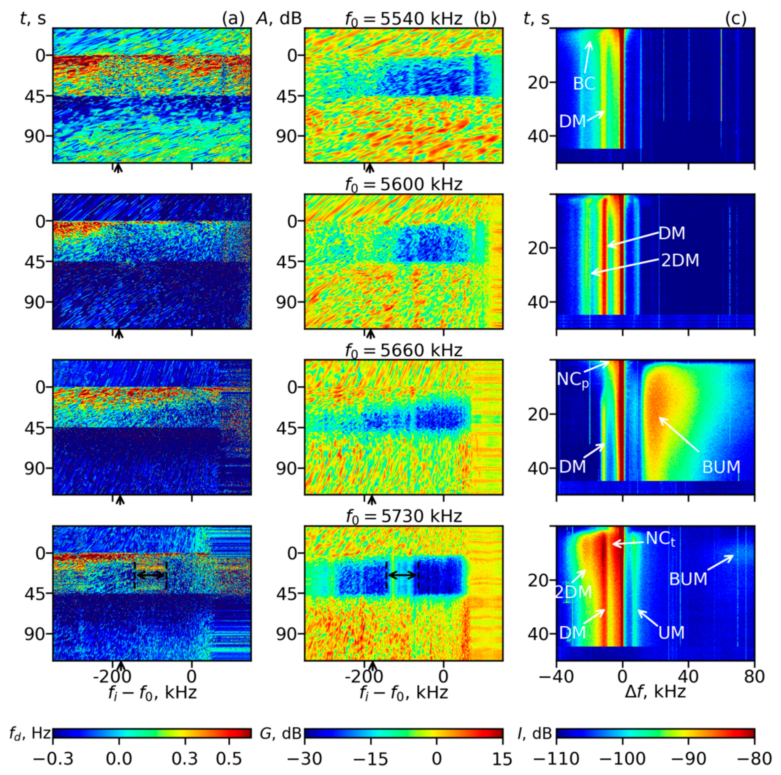
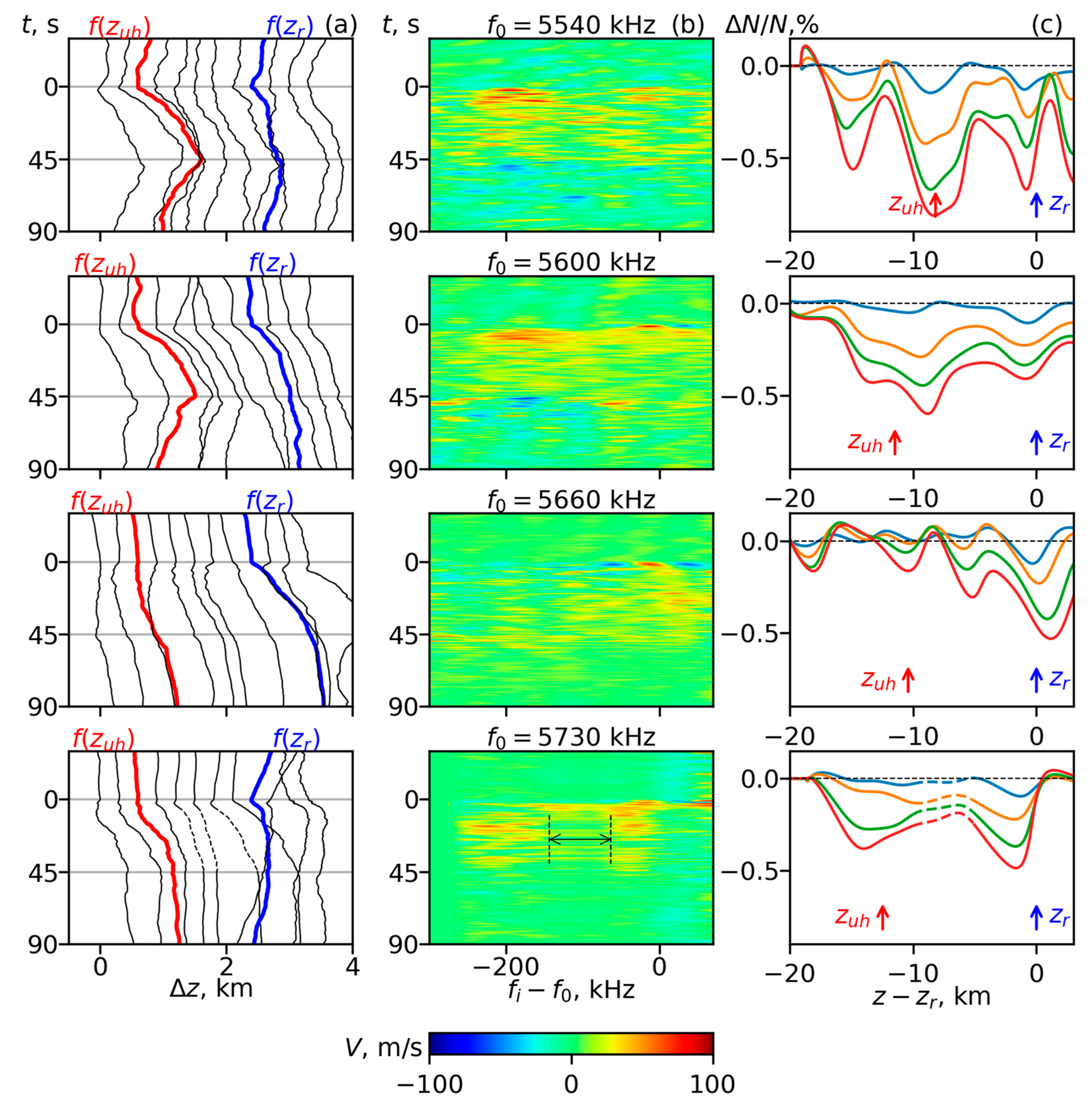
Figure 1a and Figure 3a show that immediately after the QCW was switched on, the Doppler frequency shifts noticeably increased in comparison with the background values corresponding to the natural motion of the ionosphere. They became positive (f_di > 0) for all spectral components, except for those close to the pump frequency (f_i ≈ f₀), where the f_di enlargements were weaker. Such behavior of f_di was translated into increasing the reflection altitudes of the sounding waves z_ri with the frequencies close to the pump wave frequency f₀ (Figure 2a and Figure 4a) with velocities V_v up to 100 m/s, and, in contrast, slighter decreasing z_r for both f_i > f₀ and f_i < f₀ with velocities V_v up to 60 m/s (Figure 2b, Figure 4b and Figure 5b). This corresponded to an electron density decrease in the vicinity of the pump wave reflection height z_r0 = z_r(f₀) and an increase in other heights, i.e., to the plasma expulsion from the reflection point vicinity.

The relative density depletion (hereafter reflection depletion (RD)) reaches up to ~0.1–0.2% at the fifth second of the QCW pumping (Figure 2c, Figure 4c and Figure 5c). According to Figure 2a and Figure 4a, the uplifting Δz_r(f_i ≈ f₀) grew from 0.1 s till (3–5) s, reaching 100–300 m, and then slowed down till t = 10–15 s. Note that in the cycle at f₀ = 5540 kHz, the RD depth even slightly decreased between the 10th and 15th seconds of the QCW pumping, which is clearly seen in Figure 5c.

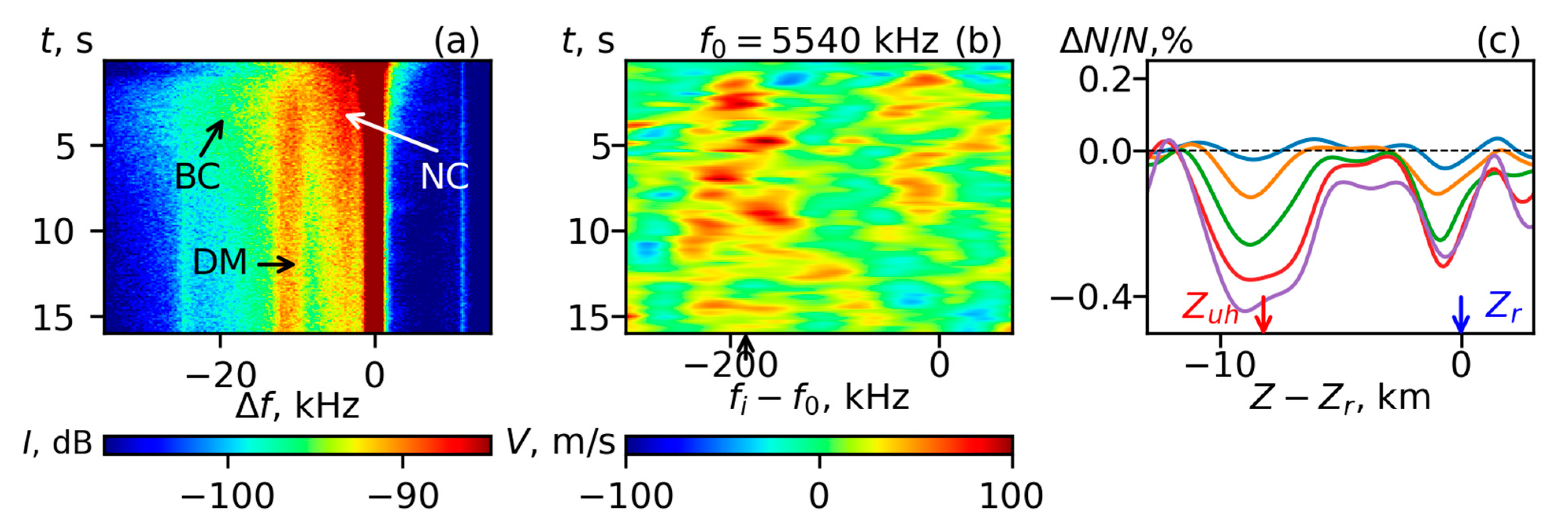
The SEE feature NC_p appeared immediately after the QCW was switched on, simultaneously with the start of the plasma expulsion from the vicinity of z_r0, and then exhibited a strong overshoot effect: its spectral width and intensity noticeably dropped during the rise in z_r(f₀) and growth of the AA- and UH-related SEE features (Figure 1b,c and Figure 5c). Such initial behaviors of the f_d(f_i, t), Δz_r(f_i, t), V_v(f_i, t), $\delta N\left(z,t\right)$, NC_p and AA were qualitatively similar for all f₀ and did not depend on the offset Δf_c.

A few seconds later, the phenomena related to the excitation of the UH waves and striations, resulting in the phenomena, such as the AA and the UH related SEE features, and the plasma expulsion from the UH height region (z~z_UH0, the “UH depletion”, hereafter UHD) developed simultaneously. At this stage, a noticeable dependence of the observed phenomena on the offset Δf_c = f₀ − 4f_c was obtained.

The following is an analysis for this time interval from the cycle with f₀ = 5540 kHz, which is shown in the upper rows of Figure 1 and Figure 2. During this cycle, the pump frequency f₀ = 5540 kHz belonged to the weak emission range between the third and fourth gyroharmonics, where the SEE spectrum contained weak BC, DM and UM (Figure 1c, row 1). In this range, the offset Δf_c = f₀ − 4f_c could be roughly estimated from the ionograms and geomagnetic field IGRF model as Δf_c ~−(130–150) kHz, where f_c should be taken at z = z_UH0, the upper hybrid resonance height of the pump wave. The AA, UH-related SEE and UHD started to develop during t = 1–3 s after the QCW was switched on. The expulsion from the UH height interval corresponded to the appearance of the expanding range with decreasing f_di near $f_p~\sqrt{f_0^2-f_c^2}~f_{\mathrm{UH}0}$ in Figure 1a, row 1. During 3–5 s, the UHD became deeper than the RD (Figure 2c, row 1, Figure 5c), and then the UHD developed monotonously till the QCW pumping was switched off. At t~15 s, the uplifting near the reflection point Δz_r(f_i ≈ f₀) accelerated again and continued till the QCW stopped; for $t\gtrsim 15$s, deepening of the UHD and RD was accompanied by a plasma density decrease in the whole altitude range $z_{\mathrm{UH}0}\lesssim z\lesssim z_{r0}$ (Figure 2c, row 1).

For the cycle at f₀ = 5600 kHz (Figure 1 and Figure 2, second row), the results of the AA measurements (temporal development and magnitude) and the phase sounding analysis (f_d(f_i, t), Δz_r(f_i, t), V_v(f_i, t) and $\delta N\left(z,t\right)$) were similar to those for f₀ = 5540 kHz, but the SEE was quite different. According to the SEE spectrogram (Figure 1c, row 2), the PW frequency belonged to the “below harmonic” range. It showed a strong DM and resolved 2DM. With the use of the ionogram and IGRF magnetic field model, the offset could be roughly estimated as Δf_c ~−(60–70) kHz. According to the ionograms, the $z_{\mathrm{UH}0}$ values in the cycles at 5540 and 5600 kHz were close at $z_{\mathrm{UH}0}~225\mathrm{km}$. During these cycles in the DW frequency range $-220<f_i-f_0<-170$ kHz, the average anomalous absorption $|\langle G\rangle |$ was smaller by ~10–15 dB (Figure 1b) in comparison with the range $-30<f_0-f_i<$ 150 kHz. Note that the reflection height of the DW with $f_i~f_0-180$kHz was approximately equal to the PW UH height $z_{r_i}~z_{U{H}_0}$, where $f_p~\sqrt{f_0^2-f_c^2}~f_{\mathrm{UH}0}$. This frequency is shown in Figure 1a,b, Figure 2b, Figure 3a,b, Figure 4b and Figure 5b by an arrow below the abscissa axis.

In the cycle at f₀ = 5660 kHz (Figure 1 and Figure 2, 3rd row), the behavior of the bulk of investigated parameters differed noticeably from the cycles at f₀ = 5540 and 5600 kHz, as well as from the cycle at f₀ = 5730 kHz (see below). In this cycle, the RD developed similar to the cycles with other f₀ values during the first 10 s of the QCW pumping but it did not slow down after t = 10 s. Smallest values of f_di appeared initially in the range surrounding f_i (z_r0), then this range expanded mainly to lower f_i. The dependence on δN(z) looked like a shallow quasi-periodic structure that occupied a height interval that exceeded the spacing between z_r0 and z_UH0 with a period~3–4 km and an amplitude that grew in time and decreased along z downward from z_r0 (Figure 2c)_. The UHD and z_UH0 uplift did not resolve in this cycle. Moreover, a weak decrease of the reflection heights $z_{r_i}\left(f_i\right)$ for frequencies surrounding $f_{\mathrm{UH}0}=f_i\left(z_{{\mathrm{UH}}_0}\right)$ was observed. Then, the AA and NCp overshoot developed slower than in other cycles, while the AA attained the same magnitudes as for f₀ < 4f_c till the 45 s of pumping. The difference was due to the fact that during this cycle at f₀ = 5660 kHz, the PW frequency belonged to the resonant range. This was seen from the SEE spectrogram (Figure 1c). Here, the DM was not resolved till t ~10–15 s, which means that

f_DM = f₀ −Δf_DM ≈ f_UH0 ≈ 4f_c,

(8)

at the PW UH height, i.e., the DM peak frequency f_DM was in the double resonance. Then, the DM appeared, which was probably attributed to the amplification of the $\mathsf{\delta }N\left(z, t\right)$, changing of the UH height and, therefore, to a violation of Equation (8). This allowed for estimating the offset Δf_c = f₀ − 4f_c during the cycle as 7–15 kHz; initially, Δf_c ≈ Δf_DM and then changed. Detailed analyses of the SEE peculiarities (DM, UM and BUM) near the double resonance can be found in [11,14,18,26]. Note that the altitude of the double resonance obtained from Equation (8) and the IGRF model was ~240 km and exceeded the z_UH0 that was obtained from the ionogram by ~10 km. However, this value fits into the error bar when determining the heights when processing the ionograms.

The cycle at f₀ = 5730 kHz (Figure 1 and Figure 2, 4th row) was the only cycle with f₀ > 4f_c (above harmonic range). Here, the offset Δf_c = f₀ − 4f_c at the BUM SEE feature generation height z_BUM could be estimated from the SEE spectrogram (Figure 1c, 4th row) as

Δf_c = f₀ − 4f_c ≈ f_BUM − f₀ = Δf_BUM, Δf_c~+75 kHz,

(9)

where f_BUM is the BUM peak frequency. According to the IGRF magnetic field model z_BUM ~238 km, which exceeded, again, the z_UH0 that was obtained from the ionogram by a few kilometers.

From Figure 1 and Figure 2 for f₀ = 5730 kHz (4th row), the following can be concluded. After the QCW pumping, switching on the plasma expulsion from the vicinity of the reflection point (RD) and the NC_p development in the SEE spectrum behaved similarly to all f₀. Slowing down of the RD deepening after the development of the UH-related effects was not observed. Like for f₀ < 4f_c, for f₀ > 4f_c, the UH-related effects (AA, DM, 2DM, UM SEE features and UHD) developed a few seconds later than the L-related processes near the reflection height. However, the characteristics of these processes during the cycle differed from the ones for f₀ < 4f_c. First, for f₀ > 4f_c, the AA was stronger, developed faster than for f₀ < 4f_c and f₀ ≈ 4f_c. It attained a saturation $|\langle G\rangle |~$25–30 dB at t $\gtrsim$ 10–15 s, while for f₀ < 4f_c (f₀ = 5540 kHz and 5600 kHz), $|\langle G\rangle |~$18–20 dB at t $\gtrsim$ 20 s was produced, and at the double resonance case (f₀ = 5660 kHz), $|\langle G\rangle |$ ~18–20 dB at t $\gtrsim$ 25 s was produced. The DW frequency range with a strong AA was wider at f₀ > 4f_c than at f₀ < 4f_c (Figure 1b). Due to the strong AA, in the range 5590 < f_i <5650 kHz, the DW signal intensity decreased to the background noise, and measurements of the Doppler shifts/phase incursions and AA became impossible due to noise interference. This range is shown in Figure 1 and Figure 2, row 4, by double arrows and dashed parts of the lines. It shall be excluded from the analysis for t >15 s. Second, a strong NC_t showed up in the SEE spectrogram at$\Delta f~0-\left(-7\right)$kHz with a temporal behavior that was similar to the DM, 2DM and UM; after t~1.5 s, the NC_t covered NC_p. The DM, 2DM and UM developed concurrently with the AA and exhibited an overshoot effect with maxima at t~6–11 s. These SEE features were more intense than in other cycles. Such SEE behavior is typical for the above harmonic range close to the strong emission range [14]. Third, the UHD started to develop at ~2 km above the nominal upper hybrid resonance height z_UH0 and occupied quite a wide (>5 km) altitude interval. Later, during t~10–15 s, the interval expanded (till ~8 km) and descended below the UH height. During the whole 45 s of the QCW pumping, the UHD remained shallower than the RD (Figure 2c, 4th row).

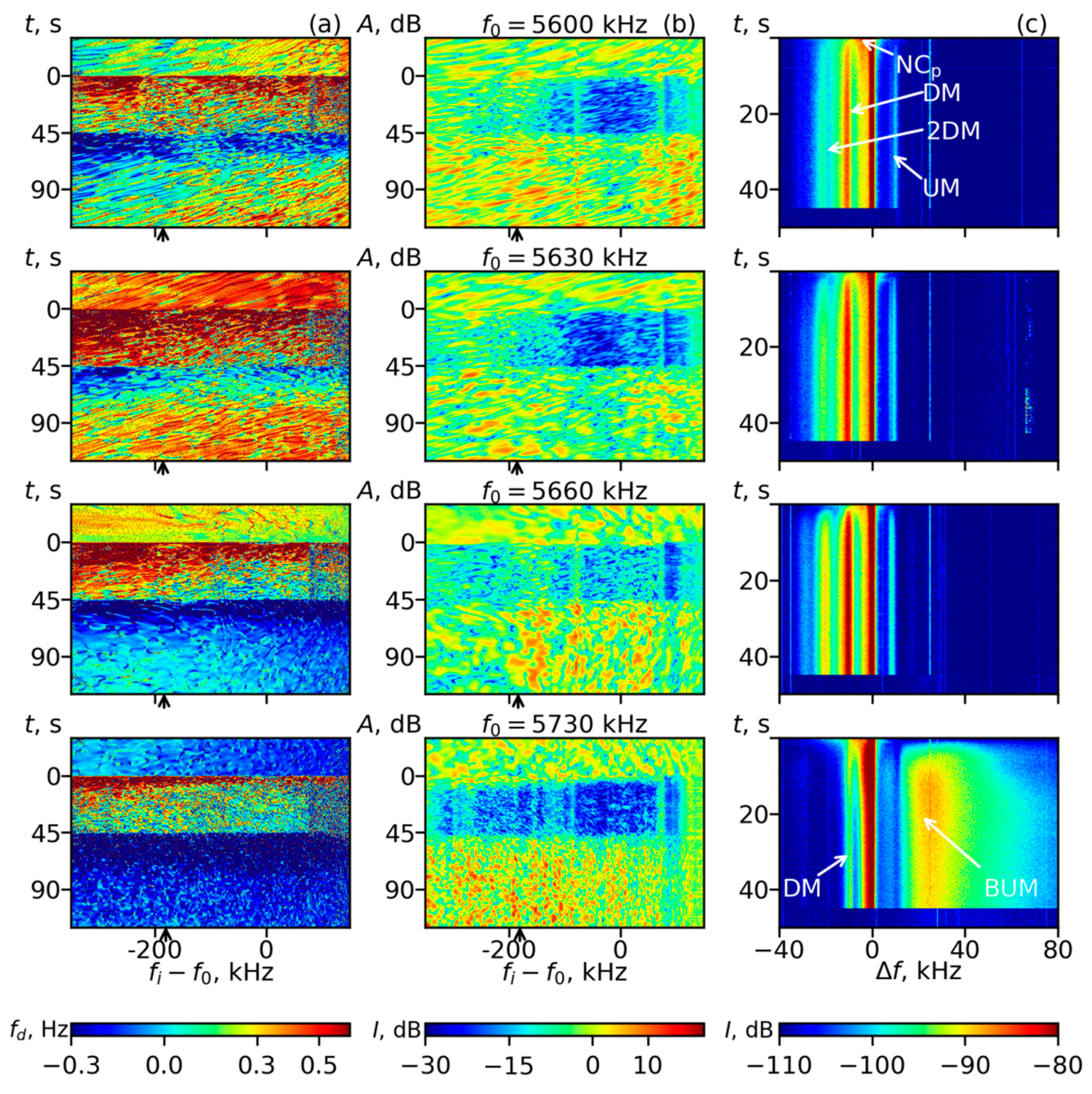
The four cycles described above were collected during 14:55–15:15 and 16:00–16:05 AKDT. During the cycles performed during 16:05–16:25 AKDT, the ionosphere descended, the PW reflection heights z_r0 were lower, i.e., z_r0~215–225 km, and the nominal values of the fourth gyroharmonic were larger by 50–70 kHz. The results of these four cycles are shown in Figure 3 and Figure 4. During the first three cycles (f₀ = 5600, 5630 and 5660 kHz), the PW frequencies were f₀ < 4f_c; in the last cycle (f₀ = 5730 kHz), f₀ $\gtrsim$ 4f_c. According to the SEE spectrograms (Figure 3c), the PW frequency f₀ = 5600 kHz (upper row) was in between the weak emission range and below harmonic range: the DM and UM were weak but stronger than at f₀ = 5540 kHz, and the 2DM was barely resolvable. For an increase in f₀ by 30 kHz in each of the next two cycles (f₀ = 5630 kHz and 5660 kHz), the PW frequencies belonged to the below harmonic range) and f₀ approached 4f_c from below. This was confirmed by amplification of the DM, 2DM and UM in the spectrograms (Figure 3c). Using the ionograms and IGRF model, the offsets Δf_c during the three cycles with f₀ < 4f_c could be roughly estimated as Δf_c~−(110–130), −(90–100) and −(55–65) kHz. Note that the SEE spectrogram in Figure 1c at f₀ = 5600 kHz was similar to the ones at f₀ = 5630 kHz in Figure 3c. This shows that the offsets Δf_c were close in these cycles. This happened because of a decrease in the ionosphere and an increase in the magnetic field strength at the lower heights.

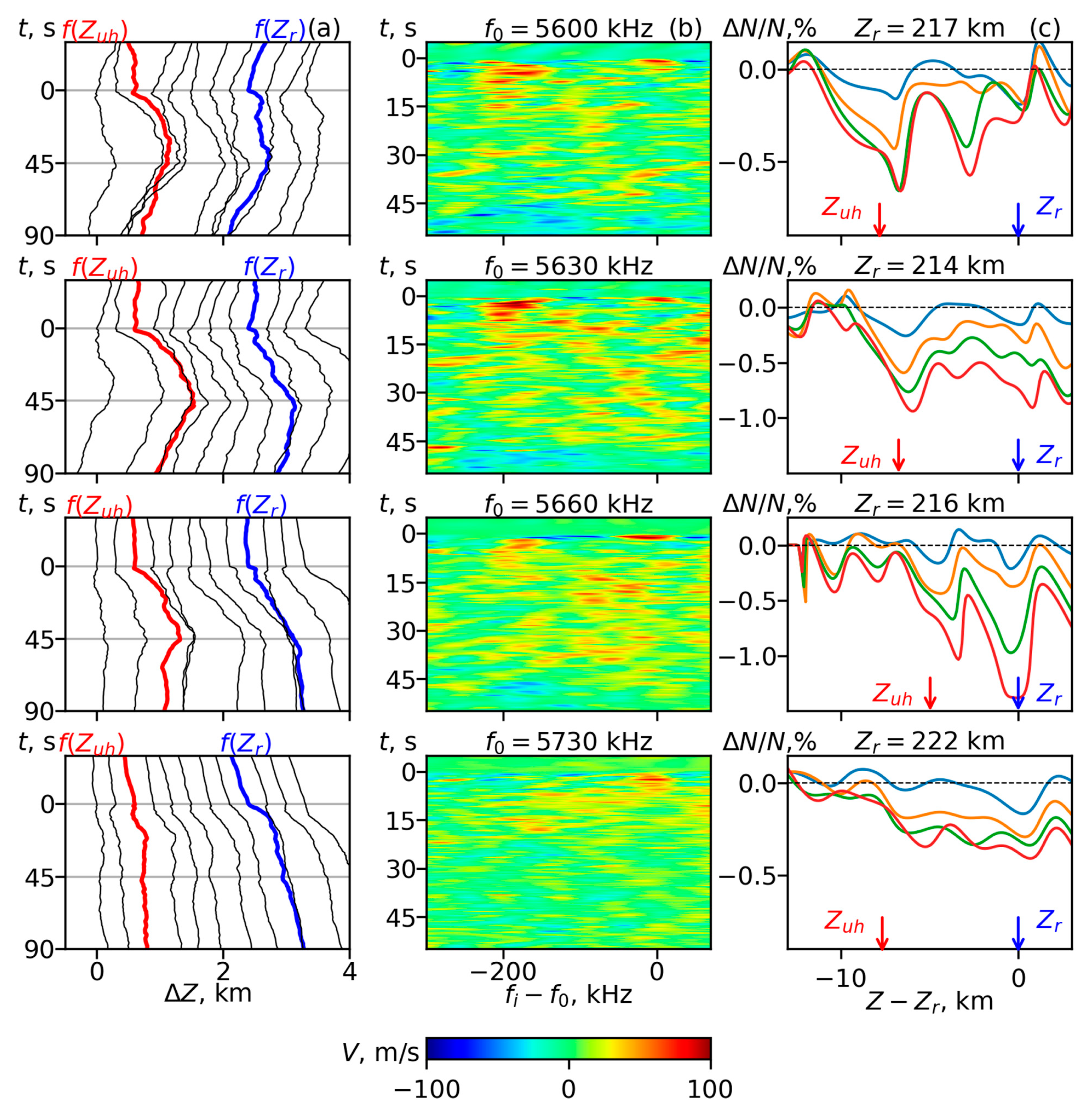
For the three cycles with f₀ < 4f_c, the temporal behavior of f_i, AA, SEE, $z_{r_i}$, V_v and δN were qualitatively similar to those for larger PW reflection heights: Initially, the plasma expulsion from the PW reflection height (RD) and NC_p SEE spectral feature developed. Then, for $t\gtrsim 1-3$s, the UH-related phenomena (AA, DM, UM, 2DM and UHD) developed concurrently with the NC_p overshoot and the RD deepening slowed down, and the UHD became deeper than the RD (at $t\gtrsim 3-5$s). The AA also dropped by 10–15 dB in the DW range $f_i~ f_{\mathrm{UH}0}$. Then, the uplifting near the reflection point Δz_r(f_i ≈ f₀) accelerated again and continued till the QCW stopped, and for $t\gtrsim 15$s, deepening of the UHD and RD was accompanied by a plasma density decrease in the whole altitude range $z_{\mathrm{UH}}\lesssim z\lesssim z_{r0}$. The difference between these cycles and the cycles shown in Figure 1 and Figure 2 lies in the fact that in the below harmonic range for the close offsets $\Delta f_{\mathrm{c}}$, the UHD turned out to be deeper for low altitudes of the ionosphere. In particular, at f₀ = 5600 kHz (Figure 2c) at the end of pumping (t~45 s), δN was 0.6%, while at f₀ = 5630 kHz and 5660 kHz (Figure 4c), δN attained 1–1.05%. At the same time, the uplifting of the UH height $\Delta z_r\left(f_{\mathrm{UH}}\right)$ remained nearly the same with $\Delta z_r\left(f_{\mathrm{UH}}\right)$ ~750–900 m (Figure 2a and Figure 4a). At the PW frequency that belonged to the weak emission range for different ionosphere heights (Figure 2, f₀ = 5540 kHz, 16:00 AKDT and Figure 4, f₀ = 5600 kHz, 15:00 AKDT), the UHD depths were close (δN~0.7–0.8%) while the UH height uplift was larger for the higher ionosphere. The plasma density reduction in the whole altitude range $z_{\mathrm{UH}0}\lesssim z\lesssim z_{r0}$ as well as the RD deepening at t = 15–45 s was greater for lower ionosphere heights. The greatest reflection point uplift occurred at f₀ = 5630 kHz (16:15 AKDT) and f₀ = 5660 kHz (16:10 AKDT) and achieved 500–600 m, while the relative depth of the RDs $\mathsf{\delta }N\left(z\approx z_r\right)$ for these two cycles attained 0.9 and 1.3%, respectively. Note that in the cycle at f₀ = 5660 kHz, the RD depth exceeded the UHD depth for t > 20–25 s (Figure 4c). Furthermore, in this cycle, the AA was the smallest with $\langle G\rangle ~10$ dB.

The pump frequency f₀ = 5730 kHz (Figure 3 and Figure 4, 4th row, 16:20 AKDT) belonged to the lower frequency flank of the above harmonic range near the resonance range $f_0\gtrsim 4f_{\mathrm{c}}$. This is seen in Figure 3c, 4th row: in the SEE spectrogram, the weak DM and UM, as well as the BUM with a peak at Δf_BUM~25 kHz, were present. Here, f_c could be estimated from Equation (9) as f_c ≈ 1426 kHz, which corresponded to a height of z ≈ 220 km. In this cycle, the behavior of the investigated parameters was very close to one that was obtained in the cycle at f₀ = 5660 kHz (Figure 1 and Figure 2, 3rd row, 15:10 AKDT). Here, again, the dependence on δN(z) looked like a shallow quasi-periodic structure starting near z_r0, expanding to a lower z and occupying a height interval that exceeded the spacing between z_r0 and z_UH. The difference between these two cycles was that the amplitude of the quasi-periodic structure was smaller in the cycle at a lower ionosphere, where during t~15–25 s, the small UHD could be resolved (see Figure 4a); in this cycle at f₀ = 5730 kHz, the AA developed faster than at f₀ = 5660 kHz but achieved close stationary values.

After the termination of the QCW, the Doppler frequency shifts f_di dropped sharply and became negative for the majority of the cycles. This led to a reduction in the pump-induced plasma density depletions around the reflection and UH heights, the depletions relaxed and disappeared during ~15–40 s after the QCW pumping turned off and the plasma motion was determined by natural causes.

4. Discussion and Conclusions

In this article, we present experimental results from the HAARP ionospheric research facility (Gakona, Alaska, USA) that were produced when studying plasma density profile modifications in the F-region caused by HF pumping with the frequency f₀ in the range [(−150 kHz)–(+75 kHz)] around the fourth electron gyroharmonic 4f_c. The specially elaborated pump wave radiation schedule was used for multi-frequency Doppler sounding of the HF-pumped volume of the ionosphere. Measurement of the phases and amplitudes of the reflected diagnostic signals was complemented by the observations of the SEE.

The main results of the study can be summarized as follows.

It was obtained that during all cycles, the pump wave–plasma interaction developed most quickly (in a few milliseconds) after the QCW switched on in the vicinity of the pump wave reflection height z_r0. This was accompanied by the plasma expulsion from the interaction region (RD appearance), uplifting of the PW reflection point and the NC_p SEE feature generation. At this time, there were no essential differences between the cycles with different f₀. Both the expulsion and NC_p were attributed to the excitation of L-waves due to the ponderomotive parametric instability near the PW reflection height z_r0. Here, the L-waves propagated almost along the (geo)magnetic field B. The dispersion properties of the L-waves and, therefore, the NC_p and RD dynamics practically did not depend on the proximity of the PW frequency f₀ to 4f_c. The absence of the NC_p dependence on $f_0-n{f}_{\mathrm{c}}$ at the initial stage of pumping for n = 4, 5 was discussed by [17,19,25,26]. The RD dependence on $\Delta f_{\mathrm{c}}$ was investigated in the presented study for the first time.

Later, during the 1–5 s after the QCW was switched on, for f₀ < 4f_c, the plasma expulsion from the vicinity of the upper hybrid height z_UH0 (UHD development) began, along with the development of the AA; UH-related SEE features, such as DM, 2DM, UM and BC; and the suppression (overshoot) of the NC_p feature and slowing down of expulsion from the vicinity of z_r0. During 3–10 s, the UHDs became deeper than the RDs. The expulsion from the upper hybrid height continued until the end of the 45 s long QCW pumping. All these effects were related to the excitation of the striations and UH plasma waves under the thermal parametric instability. The slowing down of the z_r0 uplifting, RD deepening (and even slight decrease of the RD depth during the cycle at f₀ = 5400 kHz during t = 10–15 s) and NC_p suppression indicated that the UH-related processes led to noticeable shielding of the reflection point from the pump wave energy. The sequence of the described effects was consistent with the general scenario of the phenomena developing in the HF-pumped ionosphere [2,17,33], which was clearly illustrated by [37], where the results of three successive 2 min cycles of pumping organized in a similar way at the frequency f₀ = 5500 kHz obtained using the same experiment (4 June 2014, 15:40–15:46 AKDT) were presented. Similar results were also obtained at the “Sura” facility [9]. In the described experiment, during the cycles at f₀ < 4f_c, the RD and NC_p developed similarly to the cycles at f₀ = 5500 kHz till t = 5–10 s, but later ($t\gtrsim 15$ s), the RD started to deepen again, concurrently with the UHD deepening on the background of plasma density decrease in the whole height interval $z_{\mathrm{UH}0}\lesssim z\lesssim z_{r0}$. The dependence on $\mathsf{\delta }N\left(z\right)$ looked like two isolated minima close to the reflection height$z_{r0}$ and the UH height $z_{\mathrm{UH}0}$, respectively.

Note that for cycles at f₀ < 4f_c with approximately the same initial UH heights of $z_{\mathrm{UH}0}$~225 km, the expulsion parameters $\Delta z\left(f_i\right) \mathrm{and} \delta N\left(z\right)$, as well the AA, behaved similarly, even quantitatively, while the SEE spectra were different (Figure 1 and Figure 2, rows 1, 2). This pointed to a weak dependence of the AIT peculiarities on $\Delta f_c$ in the range $-150 \mathrm{kHz}\lesssim \Delta f_c\lesssim -60$ kHz. For the smaller initial UH heights (Figure 3 and Figure 4, rows 1–3) $z_{\mathrm{UH}0}$~207–211 km, for Δf_c~−(55–100) kHz, the UHD and RD developed until noticeably larger depths. Furthermore, for f₀ = 5630 kHz (Δf_c~−(90–100) kHz), the RD attained approximately the same depth as the UHD, while for f₀ = 5660 kHz (Δf_c~−(55–65) kHz, closer to 4f_c), the RD became even deeper than the UHD. The latter probably happened because in this cycle, the anomalous absorption was $|\langle G\rangle |$~ 10 dB, which was 2–3 times less than in other cycles. Hence, the energy loss near the UH height due to the DW (and PW) energy transfer to the plasma (UH) waves on the striations was also less, and the larger portion of the PW energy was delivered to the reflection height and effectively contributed to the RD deepening.

In the single cycle with f₀ > 4f_c (above harmonic range near the strong emission range, Figure 1 and Figure 2, 4th rows, f₀ = 5730 kHz, $\Delta f_{\mathrm{c}}~75$ kHz), the $\mathsf{\delta }N\left(z\right)$ developed, again, as two isolated minima, namely, RD and UHD. In this cycle, the UHD depth remained less than the RD depth during the whole OCW pumping interval; the altitude ranges that were occupied by the depletions were wider, while the AA of the DW was stronger (by ~10 dB) and occupied a larger frequency range than in the cycles with f₀ < 4f_c. The uplifting of the DW reflection heights z_ri near the PW UH height started at a t~15 s delay (Figure 2c, row 4) after the QCW was switched on. This pointed to the essential difference in the AIT excitation between the cases f₀ > 4f_c and f₀ < 4f_c. Note that the stronger AA for f₀ > 4f_c than for f₀ < 4f_c was noted in [7,21,22].

In the cycle at f₀ = 5660 kHz (Figure 1 and Figure 2, rows 3), the PW frequency was close to 4f_c, i.e., it got into the resonance range, where the DM was totally suppressed or very weak, but the BUM and UM were present in the SEE spectra. Taking f_DM = f₀ − Δf_DM ≈ 4f_c(z_UH) ≈ 5650 kHz and using the IGRF model for the geomagnetic field, we obtained z_UH0 ≈ 239 km at the beginning of the cycle. In this cycle, the DW frequency range with a negative f_di expanded from the PW frequency f₀ (Figure 1a, 3rd row), the temporal behavior of $\mathsf{\delta }N\left(z, t\right)$ demonstrated a deepening quasi-periodic structure with a period ~3–4 km and an amplitude that grew in time and went downward from z_r0 and occupied a height interval that exceeded the spacing between z_r0 and z_UH0. Unfortunately, the total range of the diagnostic signals that were available for the phase data processing was too narrow to estimate the lower boundary of the height interval. “Independent” z_ri uplifting for z_ri~z_UH0 was not resolved in this cycle. Therefore, for f₀ ≈ 4f_c, the plasma expulsion from the UH region, as well as the DM generation, were quenched, and the total PW energy flux practically achieved the PW reflection point z_r0. The AA, and hence the striations, developed slower than at f₀ far from gyroharmonic, concurrently with the appearance of the weak DM in the SEE spectrum, but $|\langle G\rangle |$ attained quite large values of ~20 dB till the end of QCW pumping in the DW frequency range −150 kHz< f_i−f₀ < 50 kHz (Figure 1b). In the cycle at f₀ = 5730 kHz (16:20 AKDT, Figure 3 and Figure 4, row 4), the PW frequency was found in the low-frequency flank of the above harmonic range, close to the resonance range $f_0\gtrsim 4f_{\mathrm{c}}$. Here, the temporal behavior of $\mathsf{\delta }N\left(z, t\right)$ also demonstrated deepening quasi-periodic structure with a period~3–4 km, but during t~15–25 s after the PW switch on the small UHD could be resolved. Moreover, the AA developed faster than at f₀ = 5660 kHz (compare Figure 1b, 3rd row and Figure 4b, 4th row).

Assuming that the height of the greatest plasma expulsion corresponds to the maximum PW energy consumption by ionospheric plasma, we can conclude that the most effective PW energy input occurred initially near the PW reflection height z_r0. Later, for f₀ < 4f_c, the energy input became more effective near the UH height z_UH0. Then, when the plasma expulsion developed throughout the whole region $z_{\mathrm{UH}0}\lesssim z\lesssim z_{r0}$, the mutual influence of these two separated regions was, presumably, observed. For f₀ > 4f_c, these two isolated regions remained independent, although the UHD occupied a greater altitude range. The difference in the UHD behavior above and below the gyroharmonic was attributed to the different dispersion properties of plasma (UH) waves with a frequencies f > 4f_c and f < 4f_c and, therefore, different efficiencies of their excitation at different $\Delta f_c$ values [11,19,26]. Deeper and more concentrated UHDs at f₀ < 4f_c also provided a decrease in the average anomalous absorption $|\langle G\rangle |$ in the DW range $-220<f_i-f_0<-170$ kHz, which is seen in Figure 1b and Figure 3b and noted above. This could be attributed to the focusing of the HF diagnostic radio waves that were reflected from the UH altitudes with density depletion [4].

For f₀ ≈ 4f_c, the PW energy was delivered mainly near $z_{r0}$ and the AIT excitation near the UH height $z_{\mathrm{UH}0}$was suppressed. The slower AA (and striations) development may indicate that in the resonance range, the slowly developing striations with relatively large scales transverse to the magnetic field (say 15–30 m) experienced less suppression (if any) than the striations with smaller scales (say 2–15 m). A similar phenomenon, namely, more the important role of the larger striations in the DM generations for small offsets Δf_c = f₀ − 5f_c, was mentioned by [20].

A reason for the observed plasma expulsion is the enhancement of the electron gas-kinetic pressure due to electron heating and the averaged high-frequency (ponderomotive) pressure. The enhancement is conditioned by the excitation of plasma (L and UH) waves by the pump wave near its reflection and UH heights. The stationary distribution of the plasma density over height z is considered in [39,40,41]. We estimated the dynamic behavior of the plasma expulsion from the altitudes of the plasma wave excitation using a one-dimensional system of transport equations. The system included an (i) electron thermal conductivity equation that took account of the electron cooling and the source related to the ohmic heating of electrons by pump-induced plasma (L and/or UH) waves, and an (ii) ambipolar diffusion equation for the electron density that took account of the thermal diffusion, electron lifetime and the term related to the ponderomotive pressure of the pump-induced plasma waves. Simple model calculations showed that the ponderomotive pressure of the excited plasma (L and UH) waves was responsible for the “independent” RD and UHD appearance and development, while the ohmic heating provided an alignment of the electron temperature along extended height interval that exceeded a distance between $z_{\mathrm{UH}0}$ and $z_{r0}$, as well as the slow plasma expulsion observed in the whole interval $z_{\mathrm{UH}0}\lesssim z\lesssim z_{r0}$ [42]. A complete description of the electron density profile modification dynamics near PW resonances requires further theoretical efforts.

Finally, combined investigations of the HF heated volume by MDS, SEE and AA allowed for establishing the interconnection between different manifestations of the AIT and determining the position (altitude) of the most effective pump wave energy input in the HF-pumped ionosphere with respect to the offset between f₀ and nf_c. However, such experiments require stable ionospheric conditions (at least during 1.5–2 h) for avoiding uncontrolled changes in the pump wave reflection and upper hybrid heights, namely, $z_{r0}$ and $z_{\mathrm{UH}0}$, where the pump–plasma interaction is known to be strongest, and therefore the frequency offset $\Delta f_{\mathrm{c}}=f_0-n{f}_{\mathrm{c}}$ near $z_{\mathrm{UH}0}$, the transport (thermal conductivity and diffusion) coefficients and the presence of the PW reflection.