Article

Mapping Cropland Burned Area in Northeastern China by Integrating Landsat Time Series and Multi-Harmonic Model

1
School of Information Engineering, China University of Geosciences, Beijing 100083, China
2
School of Biological Sciences, Faculty of Science, University of Hong Kong, Hong Kong SAR, China
3
Department of Geosciences and Geography, University of Helsinki, P.O. Box 68, 00014 Helsinki, Finland
4
State Key Laboratory of Information Engineering in Surveying, Mapping and Remote Sensing, Wuhan University, Wuhan 430079, China
5
Institute for Atmospheric and Earth System Research, Faculty of Science, University of Helsinki, 00014 Helsinki, Finland
*
Author to whom correspondence should be addressed.
Remote Sens. 2021, 13(24), 5131; https://0-doi-org.brum.beds.ac.uk/10.3390/rs13245131
Submission received: 17 November 2021 / Revised: 9 December 2021 / Accepted: 14 December 2021 / Published: 17 December 2021
(This article belongs to the Special Issue Vegetation Fires, Greenhouse Gas Emissions and Climate Change)

Abstract

:
Accurate cropland burned area estimation is crucial for air quality modeling and cropland management. However, current global burned area products have been primarily derived from coarse spatial resolution images which cannot fulfill the spatial requirement for fire monitoring at local levels. In addition, there is an overall lack of accurate cropland straw burning identification approaches at high temporal and spatial resolution. In this study, we propose a novel algorithm to capture burned area in croplands using dense Landsat time series image stacks. Cropland burning shows a short-term seasonal variation and a long-term dynamic trend, so a multi-harmonic model is applied to characterize fire dynamics in cropland areas. By assessing a time series of the Burned Area Index (BAI), our algorithm detects all potential burned areas in croplands. A land cover mask is used on the primary burned area map to remove false detections, and the spatial information with a moving window based on a majority vote is employed to further reduce salt-and-pepper noise and improve the mapping accuracy. Compared with the accuracy of 67.3% of MODIS products and that of 68.5% of Global Annual Burned Area Map (GABAM) products, a superior overall accuracy of 92.9% was obtained by our algorithm using Landsat time series and multi-harmonic model. Our approach represents a flexible and robust way of detecting straw burning in complex agriculture landscapes. In future studies, the effectiveness of combining different spectral indices and satellite images can be further investigated.

1. Introduction

As a largely agricultural country, China is rich in crop straw resources, but it faces large-scale open-air cropland burning every year [1,2]. When crop straw (also referred to as crop stubble) is burned, large amounts of harmful gases are emitted, which causes air pollution, and at the same time affects the environment, air quality, traffic safety, and human health [3,4]. Compared with forest fires and grassland fires, fires in croplands occur at small scales with low-intensity burning [5,6]. Furthermore, cropland fires are randomly distributed and dispersed but present a clear seasonality [2,7]. It is difficult to obtain the large-scale spatial distribution of cropland residue burning by traditional methods such as ground surveys. Remote sensing technology is characterized by broad coverage, high temporal resolution, and low cost. Therefore, it has become the main method to monitor cropland burning [8,9].
Burned area mapping and monitoring at a global scale have been widely based on coarse spatial resolution data such as MODIS, AVHRR, and SPOT VEGETATION [10,11,12]. In addition, there are a wide variety of global burned area products that facilitated the management and environmental applications. Among them, MCD45A1, MCD64A1, and Fire_CCI are commonly used burned area products [13,14,15]. However, the coarser spatial resolution makes it impossible to monitor small burning patches such as cropland straw burning. Meanwhile, there are large omission and commission errors in the location and mapping area of the burned area product [16,17]. Cropland straw burning is the main type of open biomass burning in China and is also an important variable for calculating biomass burning emissions [1,4]. It is the largest source of error in the current biomass burning emission source inventory. Therefore, an accurate estimate of cropland burned area is necessary and needed for research and management applications.
Medium spatial resolution satellite data such as Landsat is capable to monitor cropland burned area dynamics with higher accuracy than coarse spatial resolution data and provides an ideal spatial resolution for the dynamics of cropland residue burning. In the past few years, burned area products based on Landsat images have been generated and released, including the Australian Fire Scars (AFS) product [18] and the Burned Area Essential Climate Variable (BAECV) product developed and provided by the U.S. Geological Survey (USGS) [19] that cover regional scales. The Chinese Academy of Sciences released the Global Annual Burned Area Map (GABAM) for the year 2015 [20]. However, these existing burned area products with a resolution of 30 m still cannot satisfy the demand for an accurate estimate of cropland burned area, and they have large omission and commission errors in cropland burned area monitoring [20,21]. The errors are due to the spectral similarities between burn scars and various other classes including bare soil, water, and built-up area. Hence, the use of Landsat images to accurately estimate cropland burned area remains a difficult problem.
Compared with forest fires, fires in croplands are commonly small and non-contiguous with a short duration, and cropland residue burning is a common farming practice in agricultural land management [22,23,24]. In addition, the estimation of cropland burned area is sensitive to the temporal resolution of remote sensing data, as the fires start and end at different times, making it difficult for mapping burned area through comparison between pre-fire and post-fire images. Hence, burned area detection and monitoring approaches using time series data are needed, as they can describe cropland phenological features throughout the time segment [25,26,27], and also effectively reduce the influence of cloud contamination.
Time-series approaches effectively weaken the seasonal influence of vegetation, as all phenological characteristics were modeled throughout the year. A large number of time series methods using dense Landsat time series image stacks have been widely applied to capture burned areas with the support of free access to Landsat images [18,19,28]. Recently, an algorithm integrating Landsat time series and a simple harmonic model has demonstrated good performance in mapping burned areas in a savanna area [29]. The study of the continuous change detection and classification (CCDC) method confirmed that the harmonic model can extract different land cover features, and it was developed and well-performed in monitoring land cover changes [30]. Further study of the Trend Forecast-based change detection (TFCD) method revealed that a simple harmonic model failed to capture and detect cropland changes because of the strong seasonal dynamics [31]. However, the integration of the harmonic model with Landsat time series is rarely applied in burned area monitoring over croplands where straw burning occurs frequently. Furthermore, none of these methods consider the spatial correlation of pixels’ neighborhoods, which may reduce noises generated from false detection.
Because of the diversity of land cover types and burn severity, various spectral indices have been extensively employed and evaluated for burned area monitoring [32,33], including those particularly created for burned area detection, such as the Burned Area Index (BAI) [34], the Normalized Burned Ratio (NBR) [35], and the Char Soil Index (CSI) [36], and others that can discriminate burned area from unburned as they are sensitive to vegetation changes, such as the Normalized Difference Vegetation Index (NDVI) [37], and the Global Environmental Monitoring Index (GEMI) [38]. Moreover, it was indicated from a previous study that BAI achieved the best performance in burned area detection in a savanna area using a harmonic model [33]. However, the sensitivity of BAI in burned area detection over croplands needs further investigation and evaluation.
In this study, we aim to propose a novel algorithm to identify burned areas caused by straw burning in croplands, evaluate its performance with current burned area products, and investigate how its output provides more detailed information about straw burning distribution. To achieve this goal, we integrate the multi-harmonic model with the Landsat time series to capture cropland burned pixels and adopt the land cover mask and spatial information to reduce the false detections. The proposed algorithm was tested in northeastern China where straw burning in croplands occurs frequently.

2. Material and Methods
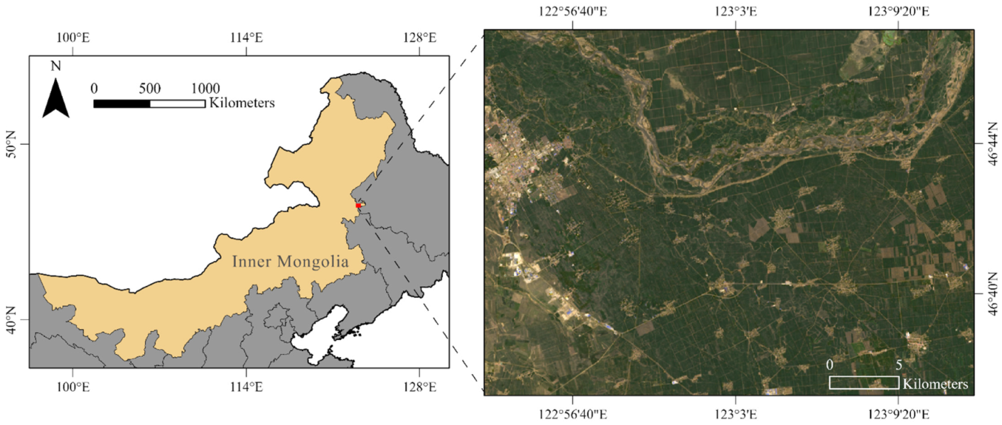
2.1. Study Area

Our study area (45°5′−45°12′W and 122°53′−123°12′E) is located in the Hinggan League, northeastern Inner Mongolia, China (Figure 1). Hinggan League is the transitional zone from Daxing’an Mountains to Songnen Plain, and this area has a typical temperate continental monsoon climate, with an average annual precipitation of 420 mm and a temperature of 5 °C. This area has a short warm summer, but a long cold winter with heavy snow from December to March. There are several land cover types, including built-up area, cropland, water, and bare land, among which cropland is the main type.
Due to constraints of climate and rainfall, maize is the most popular variety for local agricultural cultivation. Straw burning is the main method to help restore cropland after harvesting in the study area. Fire signals caused by burning activity could be captured by MODIS and Landsat data. Based on these data and the characteristics of maize planting, we find that cropland fires often occur before the snow in October to November, or after the snow in March to April in the following year. However, straw burning often causes agricultural disasters that result in economic losses and serious air pollution, and hence an accurate method of burned area detection is needed for straw burning in this area.

2.2. Data

We used a series of Landsat 8 images in our study. A total of 39 images were obtained in 2015, as we can produce the annual cropland burned area map through the time-series image stack and make a comparison with GABAM 2015 product. Details of the Landsat 8 images are shown in Table 1. All surface reflectance (SR) images of Landsat 8 were downloaded from the Google Earth Engine (GEE) platform. These images with the highest quality suitable for time series analysis were placed into Tier 1 (T1), which included L1 precision for topographical accuracy. The SR product could help detect earth surface changes by accounting for atmospheric effects. For each image, most clouds and cloud shadows were labeled and eliminated by the Fmask algorithm [39]. We selected red and near-infrared (NIR) bands for further analysis, and all images were projected into the same coordinate system (EPSG:3857).

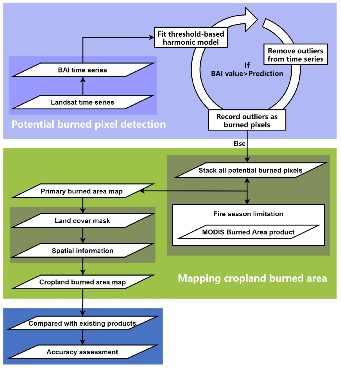
2.3. Burned Area Detection Algorithm

An overview of the cropland burned area detection algorithm is displayed in Figure 2. The whole procedure can be divided into four steps. First, we created BAI time-series data from Landsat 8 images. Next, we fitted a multi-harmonic model using the BAI time series observation values, and the outliers were determined by thresholds in the multi-harmonic regression. The outliers within the fire seasons were labeled as potentially burned pixels. Then, we combined all potentially burned pixels in fire seasons into an annual burned area map for the year 2015. A land cover mask based on a classification map with the land cover type of cropland was applied to exclude false detections, and the spatial information was used to reduce noises displayed as isolated pixels in the cropland burned area map. Finally, we carried out the stratified random sampling scheme to collect the reference data and performed an accuracy assessment by calculating the overall accuracy (OA), producer’s accuracy (PA), and user’s accuracy (UA) based on the reference data for our derived annual cropland burned area map, GABAM 2015 product, and MCD64A1 product. Details of each step are given below.

2.3.1. BAI Time Series Creation

Compared with vegetation indices, Burned Area Index (BAI) is much more accurate and successfully utilized in burned area monitoring, since BAI was developed to emphasize post-fire charcoal signal [33,40]. BAI is calculated based on red and near-infrared spectral bands, which is expressed as the following formula:
BAI = 1 ( 0.1 RED ) 2 + ( 0.06 NIR ) 2
where RED and NIR represent the reflectance in the red and near-infrared bands of Landsat 8 OLI data, respectively.
To fit the multi-harmonic model, we firstly applied the BAI formula to convert all Landsat images into BAI images. Furthermore, all clouds and cloud shadows identified by the Fmask algorithm were set into null values (NA) to avoid disturbance of abnormal values when fitting the multi-harmonic model. Then, we stacked all BAI images following their temporal orders to generate the annual BAI time series data.

2.3.2. From Single-Harmonic to Multi-Harmonic Model

A recent study indicated that the integration of sinusoidal harmonic model and time-series data could help to predict all land cover changes in a baseline period [30], and in a previous study an algorithm using a harmonic model with BAI time series data achieved satisfactory performance in burned area mapping in a savanna area [29]. Here we combined and developed the method to help detect cropland fires. The single-harmonic model is described as follows:
y t = a 0 + a 1 sin ( 2 π t T ) + b 1 cos ( 2 π t T ) + e t
where,
  • y t = predicted BAI value at Julian date t ,
  • a 0 = coefficient for overall value,
  • a 1 , b 1 = coefficients for intra-annual change,
  • t = Julian date,
  • T = number of days per year,
  • e t = remainder component.
However, the spectral characteristics of cropland had strong seasonal patterns [31]. In our study area, there were two main periods, including plowing and productive growth that generally last from May to September, harvesting and snow cover lasts from October to April. The single-harmonic model is designed for continuous monitoring of land cover changes with unimodal change, but the croplands display bimodal features due to phenology information. In addition, cropland fires demonstrate as ephemeral signals in the bimodal changes of croplands in our study area, making the simple-harmonic model invalid for burned area detection in croplands. The multi-harmonic model with six coefficients is suitable to capture surface dynamics and temporal variations in detail and has been successfully utilized in monitoring forest disturbance [41,42]. Hence, the multi-harmonic model was applied to reflect phenological features of croplands and extract burned area over croplands in the following experiments.
The samples of cropland demonstrated a bimodal trend in Figure 3. Compared with the single-harmonic model fitting curve, the samples of cropland were well fitted by the multi-harmonic model. Furthermore, the three samples with relatively high BAI values were potentially burned pixels. Therefore, a multi-harmonic model was applied to fit the intra-annual bimodal changes of cropland by using the BAI time series in our study.
The multi-harmonic model is described as follows:
y t = a 0 + a 1 cos ( 2 π t T ) + b 1 sin ( 2 π t T ) + a 2 cos ( 4 π t T ) + b 2 sin ( 4 π t T ) + e t
where,
  • a 1 , b 1 = coefficients for intra-annual unimodal change of the harmonic model,
  • a 2 , b 2 = coefficients for intra-annual bimodal change of the harmonic model.

2.3.3. Fire Season

According to the information of Ecological Environment Bureau of Hinggan League (http://sthjj.xam.gov.cn/hjzdlyxxgk/kqzl/11438.htm accessed on 8 February 2021), there were two periods of extensive and persistent straw burning in a year. The divider was the long snow cover period, which lasted from December to February and separated straw burning into two fire seasons over an agricultural cycle. Farmers had to burn the straws after harvesting in autumn, or spring before plowing, to help recover farming land. Therefore, there were two fire seasons in our study area within a year: one was the spring fire season from March to April, and the other was the autumn fire season from October to December. The intensity of the straw burning was different in the two fire seasons, and generally, the burning process was more dramatic and noticeable in the autumn fire season. The definition of fire seasons could help reduce the false detections caused by water and the built-up area in other months. To determine fire seasons more accurately, we checked MODIS burned area product which contained monthly fire date and location information, and the fire seasons it showed were consistent with those in the previous research [43].

2.3.4. Burned Area Detection

In our study area, BAI values of the non-cropland area, such as built-up area, water, and bare land are relatively small and more stable over time than those of cropland within a certain period. The values of the pixels for the burned area are abnormally high, therefore they can be detected by a certain threshold when fitting the multi-harmonic model.
The detection method included three steps. First, the BAI time series data were fitted with the multi-harmonic model (Equation (3)). Besides model parameters, we also computed the root mean square error (RMSE). Then a threshold generated from the multi-harmonic model was defined to identify the burned pixels by comparing the predicted BAI values with the observations. If the difference between observation and prediction values was larger than the threshold value, the pixel was identified as an outlier (potential burned pixel) and eliminated from the BAI time series. On the contrary, it was identified as an unburned pixel and remained. The threshold was a model predicted range aiming to separate outliers from the stable values, and was calculated as a constant value multiplied by the RMSE from the multi-harmonic model fitting. However, it was difficult to extract all burned pixels in a single regression, and we carried out the procedure repeatedly until no more outliers (potential burned pixels) were identified. In addition, only outliers within fire season were regarded as burned pixels. Finally, we unstack the BAI time series data into several separate burned area images after the iterative regression process. To derive the annual cropland burned area map, we incorporated all the burned area images in fire seasons. During the spring and autumn fire season, we set the first burned area image within fire season ranges as the reference image separately, and the remaining images were combined with the reference image by following the rule for image combination (Table 2). After the combination, a binary cropland burned area map was produced.

2.3.5. Land Cover Mask, Spatial Information and Accuracy Assessment

In our study area, water and built-up area were easily confused with burn scars due to similar BAI values [34]. However, all the burning signals should be from straw burning in the cropland. A reliable way for reducing the potential false detections is to restrict the area with a land cover mask to further minimize the negative impacts of non-cropland areas [22,44]. We used the land cover map of GLC_FCS30 in 2015, which was a land cover classification product with a resolution of 30 m [45], to extract croplands in the study area. After cropland masking, most falsely detected fire pixels in water and built-up area were removed.
The algorithm integrating Landsat time series and multi-harmonic model in our study was calculated and implemented on a pixel-by-pixel basis, and this model without considering spatial information could cause error accumulation and much noise [46]. According to Tobler’s First Law, everything is related to everything else, but those that are close to each other are more related compared to those that are distant. The majority vote algorithm applied in spatial dimensions proved to be valid to eliminate sharp noise [47]. Thus, we applied the majority vote algorithm with a 3 × 3 moving window in the spatial dimension of our derived cropland burned area map. When the number of the burned pixels in the moving window was more than four, the center pixel was labeled as burned pixel, otherwise, the center pixel was determined as unburned. However, because of the moving window filtering, burned areas below 4500 m2 are not taken into account. The majority vote method with a moving window was effective for improving the quality of classified maps, and the method with a suitable window size was able to suppress the salt-and-pepper noise caused by false detections.
It was difficult to collect reference data for the accuracy assessment of cropland burned area since cropland straw burning was geographically small and temporally dynamic. Visual interpretation proved to be effective in the accuracy assessment of the burned area in previous studies [18,29,48]. We generated 700 random samples with the random stratified sampling scheme. After we visually checked and removed incorrect points on edges, there remained 606 sample points. We interpreted all the validation sample points based on comparison with pre-fire and post-fire images to identify whether the pixel was burned or not, and the corresponding Google Earth high resolution images in the fire seasons also aided in the visual interpretation process. In addition, we considered the neighboring pixels in spatial dimension to help the visual interpretation. Based on these validation sample points, we computed OA, PA, and UA with the optimal threshold of 3 × RMSE for mapping the annual cropland burned area. We further compared our cropland burned area map with MCD64A1 burned area product and GABAM 2015 burned area product to investigate the capability of our cropland burned area detection method.

3. Results

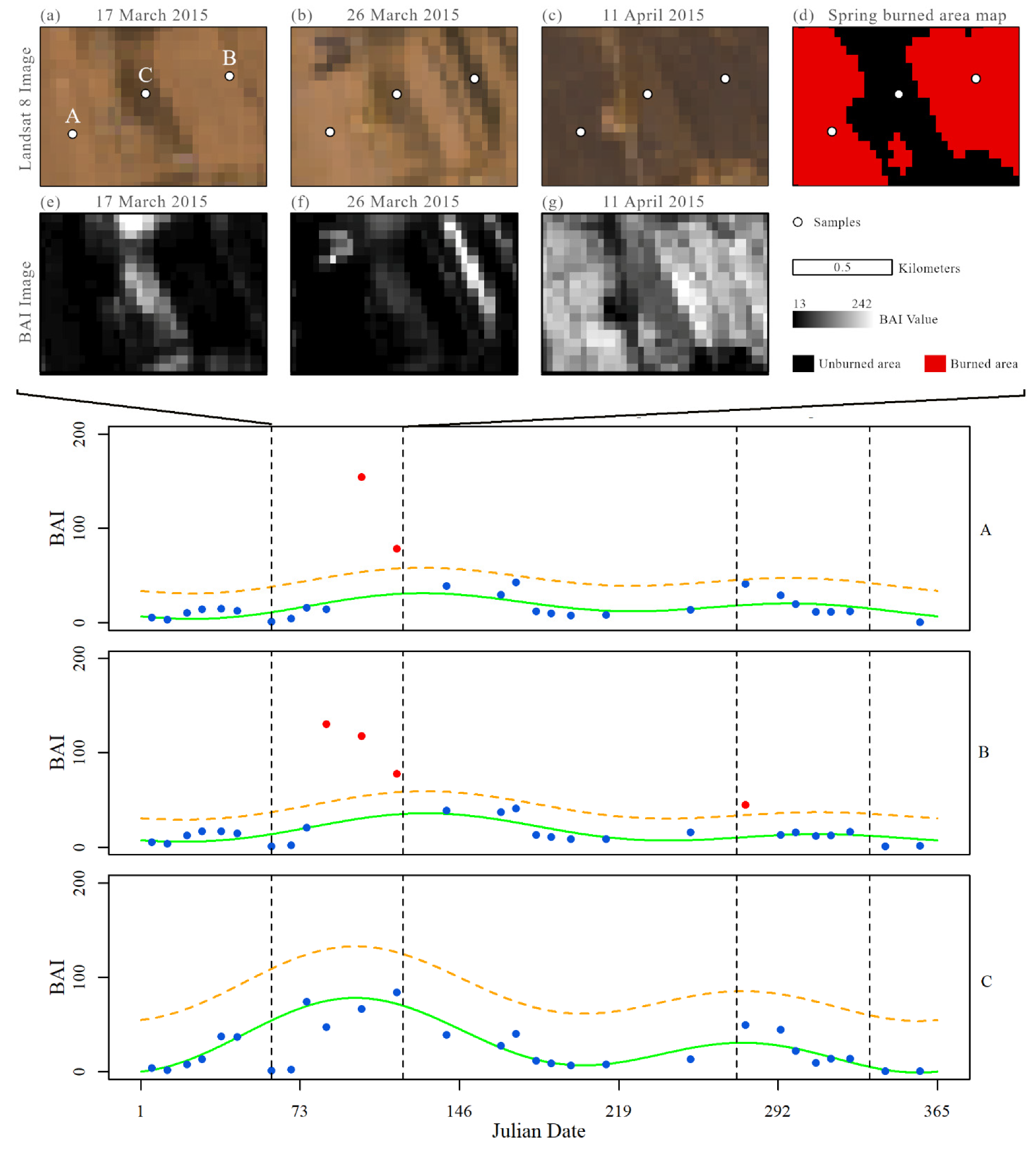
3.1. Burned Area Detection by BAI Time Series

In our study area, straw burning showed a clear temporal pattern, and it could be divided into three patterns by fire seasons within the whole year. The fire occurred only in spring or autumn, or in both periods. Figure 4 shows the process of detecting burned area for a cropland pixel time series with BAI values in the multi-harmonic model, and all burned pixels were detected after four iterations. We observed that burned pixels exhibited higher BAI values than unburned pixels, and they turned out to be outliers when fitting the multi-harmonic model. During the fourth fitting process, no burned pixels were detected, so the iteration terminated. In addition, the dates of all the detected outliers revealed that the pixels appeared during the autumn fire season in our study area, and they were regarded as potential burned pixels.
However, the difference between the old burned patches that occurred in the previous year and the unburned patches were smaller than the thresholds, so it was difficult to accurately extract the old burn scars in the fire season. Figure 5 illustrates the old and new burned patches detection in the spring fire season. We selected three points A, B, and C to illustrate the detection results with cropland pixel BAI time series. Points A and B were detected as burned pixels which occurred on 4 April 2015 and 26 March 2015, respectively, indicating a progressive burning in the spring fire season. Point C is located at the place with an old burn scar that occurred and remained from autumn fire season in the previous year, and our method was invalid to detect this type of burned pixel.
Figure 6 shows the burned area detection results for the BAI time series with different land cover types. From the three multi-harmonic model fitting curves, we observed that the trends of BAI values for built-up area and cropland were similar, leading to false detections in cropland burned area monitoring. Moreover, the water showed much higher mean and abnormal BAI values than other land cover types. Additionally, if pixels with high BAI values fall into fire seasons, then those pixels would be falsely detected and regarded as burned pixels. Thus, a land cover mask based on the land cover classification result is needed to exclude the pseudo detections in water and built-up area.

3.2. Accuracy Improvement via Land Cover Mask and Spatial Information

Figure 7 illustrates the effect of the land cover mask and spatial information on the autumn burned area map. We observed that the incorporation of land cover masks and spatial information eliminated some isolated burned pixels, and the mosaics in large burn scars were filled. Some slightly scattered burn scars were combined into larger patches. We extracted three sub-regions (A, B, and C) from the Landsat images for a demonstration in detail. The burned area maps before improvement were directly generated from the multi-harmonic model fitting algorithm without applying any accuracy improvement method, and the burned area maps after improvement were applied through the land cover mask and spatial information. For sub-regions A and B, land cover masks played a major role in reducing false detections in water and built-up area, respectively. In contrast, for sub-region C, the majority vote method considering spatial information achieved a considerable improvement in suppressing noises in unburned areas. The comparison between before and after improvement of burned area maps showed that many small scattered false detections were removed.

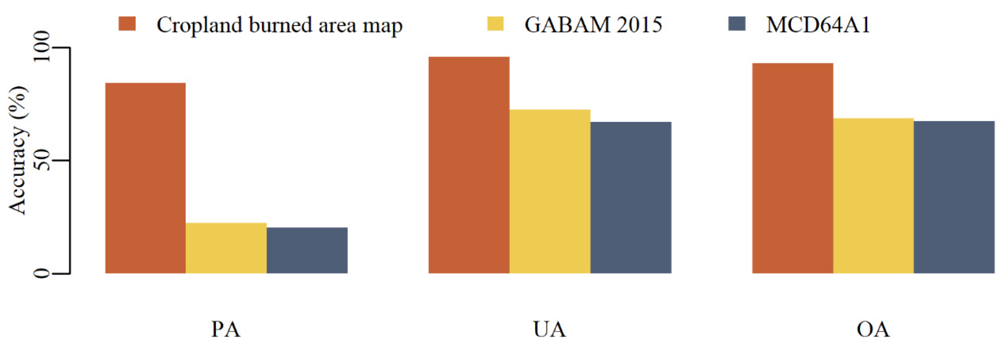
3.3. Accuracy Assessment

The performances of cropland burned area between our identification result and the other two products are compared in Figure 8. Among all the derived maps for cropland burned area, our cropland burned area map incorporating Landsat time series with multi-harmonic model achieved the highest OA of 92.9%, followed by GABAM 2015 product (68.5%), while MCD64A1 had the lowest OA (67.3%). The comparison of different products provides an insight into the agreement level between our cropland burned area result and other products in this study area. The PA and UA values demonstrated considerable variations among the three different cropland burned area detection results. The PA value for our cropland burned area result was 84.2%, much higher than PA values of 20.4% and 22.5% from the MCD64A1 product and GABAM 2015 product, respectively, indicating that our result had the capability of detecting small cropland burn scars. In contrast, small patchy burn scars were neglected and considered as unburned in products of MCD64A1 and GABAM 2015, revealing large omission errors. We clearly observed that UA values for cropland burned area derived from our method, the GABAM 2015 product and MCD64A1 product had a small variation, with values of 95.9%, 72.5%, and 67.2% respectively, suggesting lower commission errors with all the derived cropland burned area maps. The UA values were constantly higher than the PA values for the three products, however, the cropland burned area from our algorithm had a similar PA and UA value with the best accuracy performance, demonstrating a good balance between the two accuracy evaluation indices.

3.4. Comparison with MCD64A1 and GABAM 2015 Burned Area Products

Figure 9 illustrates the spatial comparison of the cropland burned area maps from our algorithm, MODIS burned area product and GABAM 2015 product in our study area. Overall, all the burned area maps shared similar spatial distribution in cropland burned area over large areas, although there are substantial differences in some small areas among different products. Specifically, cropland burned area map based on our algorithm correctly captured most smaller patches of burned area than other products. A Landsat 8 images with obvious burn scars acquired on 5 November 2015 was selected as the demonstration image, and it can be seen that the burned area map generated from our algorithm revealed a higher detection accuracy and more details than the MCD64A1 product on this specific day. In addition, large and severe burn scars clustered in the center of our study area were able to be identified by GABAM 2015 product. However, the burn scars around the corners were not observed from GABAM 2015 product, which were identified by our result. Furthermore, the MCD64A1 product failed to capture the small and fragmented burn scars because of the coarse spatial resolution.

4. Discussion

In this study, we presented a time series-based multi-harmonic model to detect cropland burned area, and the performance was compared with the products of MCD64A1 and GABAM. We observed that our results had more similarity with the other two products in large burn scars than in small and fragmented burned areas, which was consistent with previous studies [17,49]. The discrepancy between our cropland burned area and MCD64A1 product was due to the difference in spatial resolution, as the resolution of the MCD64A1 product failed to capture small and patchy burned areas, indicating the impact of a higher spatial resolution on cropland burned area mapping and monitoring. Thus, a fine spatial resolution burned area product is required for solving the problem, and the GABAM product was a global burned area map with 30 m resolution based on Landsat images and Google Earth Engine. However, the GABAM product showed a poor accuracy in capturing seasonal fires over croplands in our study area, which was similar to the results reported by Long et al. [20]. The large uncertainty in cropland burned area mapping with GABAM product was due to the spectral confusions between burned area over cropland and the area that was harvested or plowed. The multi-harmonic model we employed was sensitive to abrupt land cover changes [41], and the features of BAI in capturing post-fire charcoal signal further facilitated cropland burned area identification. The advantages of this algorithm helped us to extract not only severe and large burned scars, but also slight and fragmented ones.
The change detection method using time series data can eliminate many noises caused by the effects of cloud, cloud shadow, and snow [42]. But some pseudo burn scars were falsely detected due to the threshold in the multi-harmonic fitting process. To solve this problem, a temporal restriction accounting for the fire seasons was adopted in our cropland burned area detection method. The temporal restriction helped exclude false detections caused by mist and thin clouds outside fire seasons, which was also employed successfully for burned area detection in a savanna area by Liu et al. [29]. In addition, cropland residue burning was commonly fragmented within a short duration and less obvious given the fast vegetation recovery. Those factors made it difficult to capture small and low severity burn scars and caused omission errors. To minimize the influence of temporal resolution, two tiles (path/row: 121/027 and 120/028) of Landsat time series data were exploited to make the Landsat time series image stacks denser, which could help reduce temporal gaps for a higher observation frequency. In the future study, a combination of Landsat and Sentinel-2 datasets can provide a good opportunity to cope with the observation limitation, as the temporal resolution of combined datasets was less than 5 days [20,50].
Another error arose from the spectral dimension, as different land cover types had similar BAI values to the burned area, and a small value change could amplify the result of the index when performing band ratio operation [50], resulting in noises in our burned area map. Therefore, a land cover mask was applied to minimize the negative effect, and it was worth considering the accuracy of the land cover mask as it could directly affect our detection result. In addition, the combination of multiple spectral indices can also be an alternative to cope with the confusion between burned and unburned areas [33,51]. Moreover, some isolated false detections appeared as salt-and-pepper noises, and a spatial filter with a moving window proved to be useful for reducing the noises and refining the results by following the majority vote rule [52]. However, this method only considers simple spatial relationships within a certain distance, and it has an erosion effect in morphology, which may remove pixels on object boundaries and decrease burned area detection accuracy. So, an object-oriented algorithm considering spatial information could be applied in future studies.
The combination of Landsat time series and harmonic model was successfully conducted for burned area detection in savanna area by Liu et al. [29]. The cropland burned area results further confirmed the effectiveness of this method with a multi-harmonic model for identifying cropland burned area. Moreover, our cropland burned area detection method exhibited great potential in coping with heterogeneous burn severity patterns, as it considered the temporal features from the whole year and was sensitive to sudden changes caused by fires. Another advantage is that training sample selection is not needed in our method, and our derived result could even provide training seeds for region growth algorithm and image classification. However, the threshold value and fire season can vary spatially, and thus need to be selected and defined according to the specific region that is being analyzed. Furthermore, the lack of precise burned date is one limitation of our method, because the temporal gaps can cause lagged observations of the burning events, and also affect the detection accuracy especially when the recovery time of vegetation was shorter than the satellite revisiting period. The proposed method was successfully conducted under the assumption that no land cover changes occurred in our study area during this year. Therefore, it is recommended that this method should be applied with caution in areas where repeated land cover changes may occur.

5. Conclusions

In this study, we investigated the capacity of a multi-harmonic model based on the BAI time series in detecting burned areas over croplands in northeastern China. Our derived map of the cropland burned area from 2015 with 30 m resolution was generated with all available Landsat 8 images, and the detection result was compared with MODIS burned area product and GABAM 2015 product. Among all the detection results, our cropland burned area result based on the multi-harmonic approach outperformed the other two burned area products and revealed the effectiveness of this approach. By incorporating the fire seasons and the land cover mask based on land cover classification, the false identifications due to cloud shadows, thin clouds, and mist outside the fire seasons and non-cropland land cover areas can be further excluded, increasing the detection accuracy. Based on a spatial filter with a 3 × 3 moving window, we eliminated the isolated false detection pixels by following the majority vote rule. Our approach provides a new perspective for monitoring cropland burned areas in a timely and feasible way by incorporating temporal and spatial information. Future research should evaluate the suitability of our approach in other geographical areas and environmental conditions.

Author Contributions

Conceptualization, J.L.; methodology, J.L.; software, J.L. and D.W.; validation, J.L. and D.W.; formal analysis, J.L.; investigation, J.L. and D.W.; resources, J.L.; data curation, J.L. and D.W.; writing—original draft preparation, J.L. and D.W.; writing—review and editing, J.L., D.W., E.E.M., P.K.E.P. and J.H.; visualization, J.L. and D.W.; funding acquisition, J.L. All authors have read and agreed to the published version of the manuscript.

Funding

This research was supported by the Fundamental Research Funds for the Central Universities (grant number 2652018077). Dr Eduardo Maeda was funded by the Academy of Finland (decision numbers 318252, 319905 and 340175).

Institutional Review Board Statement

Not applicable.

Informed Consent Statement

Not applicable.

Data Availability Statement

The Landsat-8 OLI T1_SR data is downloaded from Google Earth Engine https://developers.google.com/earth-engine/datasets/catalog/LANDSAT_LC08_C01_T1_SR (accessed on 1 October 2020). MODIS Burned Area Product (MCDA64A1) is downloaded from the LP DAAC platform https://lpdaac.usgs.gov/ (accessed on 21 November 2020). MODIS Active Fire Product (MCD14DL) is downloaded from the FIRMS platform https://firms.modaps.eosdis.nasa.gov/download/ (accessed on 21 November 2020). The global land cover classification map (GLC_FCS30-2015) is downloaded from the Chinese Academy of Sciences https://0-doi-org.brum.beds.ac.uk/10.5281/zenodo.3986872 (accessed on 8 February 2021). The global annual burned area map of 2015(GABAM2015) is downloaded from the Chinese Academy of Sciences ftp://124.16.184.141/GABAM/burned%20area/ (accessed on 8 February 2021).

Conflicts of Interest

The authors declare no conflict of interest.

References

  1. Wang, L.; Jin, X.; Wang, Q.; Mao, H.; Liu, Q.; Weng, G.; Wang, Y. Spatial and temporal variability of open biomass burning in Northeast China from 2003 to 2017. Atmos. Ocean. Sci. Lett. 2020, 13, 240–247. [Google Scholar] [CrossRef] [Green Version]
  2. Xie, H.; Du, L.; Liu, S.; Chen, L.; Gao, S.; Liu, S.; Pan, H.; Tong, X. Dynamic monitoring of agricultural fires in China from 2010 to 2014 using MODIS and GlobeLand30 data. ISPRS Int. J. Geo-Inf. 2016, 5, 172. [Google Scholar] [CrossRef] [Green Version]
  3. Rabin, S.S.; Magi, B.I.; Shevliakova, E.; Pacala, S.W. Quantifying regional, time-varying effects of cropland and pasture on vegetation fire. Biogeosciences 2015, 12, 6591–6604. [Google Scholar] [CrossRef] [Green Version]
  4. Yin, S.; Wang, X.; Xiao, Y.; Tani, H.; Zhong, G.; Sun, Z. Study on spatial distribution of crop residue burning and PM2.5 change in China. Environ. Pollut. 2017, 220, 204–221. [Google Scholar] [CrossRef] [PubMed]
  5. Xia, X.; Zong, X.; Sun, L. Exceptionally active agricultural fire season in mid-eastern China in June 2012 and its impact on the atmospheric environment. J. Geophys. Res. Atmos. 2013, 118, 9889–9900. [Google Scholar] [CrossRef]
  6. Randerson, J.T.; Chen, Y.; van der Werf, G.R.; Rogers, B.M.; Morton, D.C. Global burned area and biomass burning emissions from small fires. J. Geophys. Res. Biogeosci. 2012, 117, G04012. [Google Scholar] [CrossRef]
  7. Zhang, L.; Liu, Y.; Hao, L. Contributions of open crop straw burning emissions to PM2.5 concentrations in China. Environ. Res. Lett. 2016, 11, 014014. [Google Scholar] [CrossRef]
  8. Zhuang, Y.; Li, R.; Yang, H.; Chen, D.; Chen, Z.; Gao, B.; He, B. Understanding temporal and spatial distribution of crop residue burning in China from 2003 to 2017 using MODIS data. Remote Sens. 2018, 10, 390. [Google Scholar] [CrossRef] [Green Version]
  9. Korontzi, S.; McCarty, J.; Loboda, T.; Kumar, S.; Justice, C. Global distribution of agricultural fires in croplands from 3 years of Moderate Resolution Imaging Spectroradiometer (MODIS) data. Glob. Biogeochem. Cycles 2006, 20. [Google Scholar] [CrossRef]
  10. Chuvieco, E.; Yue, C.; Heil, A.; Mouillot, F.; Alonso-Canas, I.; Padilla, M.; Pereira, J.M.; Oom, D.; Tansey, K. A new global burned area product for climate assessment of fire impacts. Glob. Ecol. Biogeogr. 2016, 25, 619–629. [Google Scholar] [CrossRef] [Green Version]
  11. Pereira, J.M.C. A comparative evaluation of NOAA/AVHRR vegetation indexes for burned surface detection and mapping. IEEE Trans. Geosci. Remote Sens. 1999, 37, 217–226. [Google Scholar] [CrossRef]
  12. Tansey, K.; Grégoire, J.M.; Stroppiana, D.; Sousa, A.; Silva, J.; Pereira, J.; Boschetti, L.; Maggi, M.; Brivio, P.A.; Fraser, R. Vegetation burning in the year 2000: Global burned area estimates from SPOT VEGETATION data. J. Geophys. Res. Atmos. 2004, 109, D14S03. [Google Scholar] [CrossRef] [Green Version]
  13. Roy, D.P.; Boschetti, L.; Justice, C.O.; Ju, J. The collection 5 MODIS burned area product—Global evaluation by comparison with the MODIS active fire product. Remote Sens. Environ. 2008, 112, 3690–3707. [Google Scholar] [CrossRef]
  14. Giglio, L.; Loboda, T.; Roy, D.P.; Quayle, B.; Justice, C.O. An active-fire based burned area mapping algorithm for the MODIS sensor. Remote Sens. Environ. 2009, 113, 408–420. [Google Scholar] [CrossRef]
  15. Chuvieco, E.; Lizundia-Loiola, J.; Pettinari, M.L.; Ramo, R.; Padilla, M.; Tansey, K.; Mouillot, F.; Laurent, P.; Storm, T.; Heil, A.; et al. Generation and analysis of a new global burned area product based on MODIS 250 m reflectance bands and thermal anomalies. Earth Syst. Sci. Data 2018, 10, 2015–2031. [Google Scholar] [CrossRef] [Green Version]
  16. Ramo, R.; Roteta, E.; Bistinas, I.; van Wees, D.; Bastarrika, A.; Chuvieco, E.; van der Werf, G.R. African burned area and fire carbon emissions are strongly impacted by small fires undetected by coarse resolution satellite data. Proc. Natl. Acad. Sci. USA 2021, 118, 9. [Google Scholar] [CrossRef]
  17. Zhu, C.; Kobayashi, H.; Kanaya, Y.; Saito, M. Size-dependent validation of MODIS MCD64A1 burned area over six vegetation types in boreal Eurasia: Large underestimation in croplands. Sci. Rep. 2017, 7, 4181. [Google Scholar] [CrossRef]
  18. Goodwin, N.R.; Collett, L.J. Development of an automated method for mapping fire history captured in Landsat TM and ETM+ time series across Queensland, Australia. Remote Sens. Environ. 2014, 148, 206–221. [Google Scholar] [CrossRef]
  19. Hawbaker, T.J.; Vanderhoof, M.K.; Beal, Y.J.; Takacs, J.D.; Schmidt, G.L.; Falgout, J.T.; Williams, B.; Fairaux, N.M.; Caldwell, M.K.; Picotte, J.J.; et al. Mapping burned areas using dense time-series of Landsat data. Remote Sens. Environ. 2017, 198, 504–522. [Google Scholar] [CrossRef]
  20. Long, T.; Zhang, Z.; He, G.; Jiao, W.; Tang, C.; Wu, B.; Zhang, X.; Wang, G.; Yin, R. 30 m resolution global annual burned area mapping based on Landsat Images and Google Earth Engine. Remote Sens. 2019, 11, 489. [Google Scholar] [CrossRef] [Green Version]
  21. Vanderhoof, M.K.; Fairaux, N.; Beal, Y.-J.G.; Hawbaker, T.J. Validation of the USGS Landsat burned area essential climate variable (BAECV) across the conterminous United States. Remote Sens. Environ. 2017, 198, 393–406. [Google Scholar] [CrossRef]
  22. Hall, J.V.; Loboda, T.V.; Giglio, L.; McCarty, G.W. A MODIS-based burned area assessment for Russian croplands: Mapping requirements and challenges. Remote Sens. Environ. 2016, 184, 506–521. [Google Scholar] [CrossRef] [Green Version]
  23. Wu, M.; Knorr, W.; Thonicke, K.; Schurgers, G.; Camia, A.; Arneth, A. Sensitivity of burned area in Europe to climate change, atmospheric CO2 levels, and demography: A comparison of two fire-vegetation models. J. Geophys. Res. Biogeosci. 2015, 120, 2256–2272. [Google Scholar] [CrossRef] [Green Version]
  24. McCarty, J.; Korontzi, S.; Justice, C.O.; Loboda, T. The spatial and temporal distribution of crop residue burning in the contiguous United States. Sci. Total Environ. 2009, 407, 5701–5712. [Google Scholar] [CrossRef]
  25. Gomez, C.; White, J.C.; Wulder, M.A. Optical remotely sensed time series data for land cover classification: A review. ISPRS J. Photogramm. Remote Sens. 2016, 116, 55–72. [Google Scholar] [CrossRef] [Green Version]
  26. Hansen, M.C.; Loveland, T.R. A review of large area monitoring of land cover change using Landsat data. Remote Sens. Environ. 2012, 122, 66–74. [Google Scholar] [CrossRef]
  27. Jia, K.; Liang, S.; Wei, X.; Yao, Y.; Su, Y.; Jiang, B.; Wang, X. Land cover classification of Landsat data with phenological features extracted from time series MODIS NDVI data. Remote Sens. 2014, 6, 11518–11532. [Google Scholar] [CrossRef] [Green Version]
  28. Liu, J.; Heiskanen, J.; Aynekulu, E.; Maeda, E.E.; Pellikka, P.K.E. Land cover characterization in west sudanian savannas using seasonal features from annual Landsat time series. Remote Sens. 2016, 8, 365. [Google Scholar] [CrossRef] [Green Version]
  29. Liu, J.; Heiskanen, J.; Maeda, E.E.; Pellikka, P.K.E. Burned area detection based on Landsat time series in savannas of southern Burkina Faso. Int. J. Appl. Earth Obs. Geoinf. 2018, 64, 210–220. [Google Scholar] [CrossRef] [Green Version]
  30. Zhu, Z.; Woodcock, C.E. Continuous change detection and classification of land cover using all available Landsat data. Remote Sens. Environ. 2014, 144, 152–171. [Google Scholar] [CrossRef] [Green Version]
  31. Chen, J.; Liu, H.; Chen, J.; Peng, S. Trend forecast based approach for cropland change detection using Landsat-derived time-series metrics. Int. J. Remote Sens. 2018, 39, 7587–7606. [Google Scholar] [CrossRef]
  32. Koutsias, N.; Pleniou, M.; Mallinis, G.; Nioti, F.; Sifakis, N.I. A rule-based semi-automatic method to map burned areas: Exploring the USGS historical Landsat archives to reconstruct recent fire history. Int. J. Remote Sens. 2013, 34, 7049–7068. [Google Scholar] [CrossRef]
  33. Liu, J.; Maeda, E.E.; Wang, D.; Heiskanen, J. Sensitivity of spectral indices on burned area detection using Landsat time series in savannas of southern Burkina Faso. Remote Sens. 2021, 13, 2492. [Google Scholar] [CrossRef]
  34. Chuvieco, E.; Martin, M.P.; Palacios, A. Assessment of different spectral indices in the red-near-infrared spectral domain for burned land discrimination. Int. J. Remote Sens. 2002, 23, 5103–5110. [Google Scholar] [CrossRef]
  35. Key, C.H.; Benson, N.C. The Normalized Burn Ratio (NBR): A Landsat TM Radiometric Measure of Burn Severity; United States Geological Survey, Northern Rocky Mountain Science Center: Bozeman, MT, USA, 1999.
  36. Smith, A.M.S.; Wooster, M.J.; Drake, N.A.; Dipotso, F.M.; Falkowski, M.J.; Hudak, A.T. Testing the potential of multi-spectral remote sensing for retrospectively estimating fire severity in African savannahs. Remote Sens. Environ. 2005, 97, 92–115. [Google Scholar] [CrossRef] [Green Version]
  37. Tucker, C.J. Red and photographic infrared linear combinations for monitoring vegetation. Remote Sens. Environ. 1979, 8, 127–150. [Google Scholar] [CrossRef] [Green Version]
  38. Pinty, B.; Verstraete, M.M. GEMI: A non-linear index to monitor global vegetation from satellites. Vegetatio 1992, 101, 15–20. [Google Scholar] [CrossRef]
  39. Zhu, Z.; Woodcock, C.E. Object-based cloud and cloud shadow detection in Landsat imagery. Remote Sens. Environ. 2012, 118, 83–94. [Google Scholar] [CrossRef]
  40. Dempewolf, J.; Trigg, S.; DeFries, R.S.; Eby, S. Burned-area mapping of the Serengeti–Mara region using MODIS reflectance data. IEEE Geosci. Remote Sens. Lett. 2007, 4, 312–316. [Google Scholar] [CrossRef]
  41. Zhu, Z.; Woodcock, C.E.; Holden, C.; Yang, Z. Generating synthetic Landsat images based on all available Landsat data: Predicting Landsat surface reflectance at any given time. Remote Sens. Environ. 2015, 162, 67–83. [Google Scholar] [CrossRef]
  42. Zhu, Z.; Woodcock, C.E.; Olofsson, P. Continuous monitoring of forest disturbance using all available Landsat imagery. Remote Sens. Environ. 2012, 122, 75–91. [Google Scholar] [CrossRef]
  43. Shan, Y.; Li, J.; Wala, D.; Jianjun, Z.; Hongyan, Z.; Qiaofeng, Z.; Huijuan, L. Estimation and spatio-temporal patterns of carbon emissions from grassland fires in Inner Mongolia, China. Chin. Geogr. Sci. 2020, 30, 572–587. [Google Scholar] [CrossRef]
  44. Bastarrika, A.; Chuvieco, E.; Pilar Martin, M. Mapping burned areas from Landsat TM/ETM+ data with a two-phase algorithm: Balancing omission and commission errors. Remote Sens. Environ. 2011, 115, 1003–1012. [Google Scholar] [CrossRef]
  45. Zhang, X.; Liu, L.; Chen, X.; Gao, Y.; Xie, S.; Mi, J. GLC_FCS30: Global land-cover product with fine classification system at 30 m using time-series Landsat imagery. Earth Syst. Sci. Data. 2021, 13, 2753–2776. [Google Scholar] [CrossRef]
  46. Li, X.; Gong, P.; Liang, L. A 30-year (1984–2013) record of annual urban dynamics of Beijing City derived from Landsat data. Remote Sens. Environ. 2015, 166, 78–90. [Google Scholar] [CrossRef]
  47. Lin, Y.; Zhang, L.; Wang, N.; Zhang, X.; Cen, Y.; Sun, X. A change detection method using spatial-temporal-spectral information from Landsat images. Int. J. Remote Sens. 2020, 41, 772–793. [Google Scholar] [CrossRef]
  48. Stroppiana, D.; Bordogna, G.; Carrara, P.; Boschetti, M.; Boschetti, L.; Brivio, P. A method for extracting burned areas from Landsat TM/ETM+ images by soft aggregation of multiple spectral indices and a region growing algorithm. ISPRS J. Photogramm. Remote Sens. 2012, 69, 88–102. [Google Scholar] [CrossRef]
  49. Fornacca, D.; Ren, G.; Xiao, W. Performance of three MODIS fire products (MCD45A1, MCD64A1, MCD14ML), and ESA Fire_CCI in a mountainous area of northwest Yunnan, China, characterized by frequent small fires. Remote Sens. 2017, 9, 1131. [Google Scholar] [CrossRef] [Green Version]
  50. Liu, S.; Zheng, Y.; Dalponte, M.; Tong, X. A novel fire index-based burned area change detection approach using Landsat-8 OLI data. Eur. J. Remote Sens. 2020, 53, 104–112. [Google Scholar] [CrossRef] [Green Version]
  51. Smiraglia, D.; Filipponi, F.; Mandrone, S.; Tornato, A.; Taramelli, A. Agreement Index for Burned Area Mapping: Integration of Multiple Spectral Indices Using Sentinel-2 Satellite Images. Remote Sens. 2020, 12, 1862. [Google Scholar] [CrossRef]
  52. Cui, G.; Lv, Z.; Li, G.; Benediktsson, J.A.; Lu, Y. Refining land cover classification maps based on dual-adaptive majority voting strategy for very high resolution remote sensing images. Remote Sens. 2018, 10, 1238. [Google Scholar] [CrossRef] [Green Version]
Figure 1. Location and demonstration of the study area. The image (true color composite) in the right panel was captured by Landsat 8 images acquired on 7 July 2015.
Remotesensing 13 05131 g001
Figure 2. An overview of the cropland burned area detection algorithm.
Remotesensing 13 05131 g002
Figure 3. Comparison of cropland pixel time series fitting results with BAI values from the single-harmonic model and multi-harmonic model, respectively.
Remotesensing 13 05131 g003
Figure 4. Demonstration of the multi-harmonic model fitting. The blue and red points represent unburned pixels and burned pixels, respectively. The green and dashed orange curves represent multi-harmonic fitting results and threshold fitting results for each regression, respectively. The vertical black dashed lines are the boundaries of fire season.
Remotesensing 13 05131 g004
Figure 5. Demonstration of cropland burned area detection in the spring fire season. The three Landsat images are selected from the spring fire season with corresponding BAI images, and the spring burned area map is the cropland burned area detection result. The three multi-harmonic model fitting graphs below are corresponding to the three points A, B, and C, respectively.
Remotesensing 13 05131 g005
Figure 6. Demonstration of cropland burned area detection with different land cover types using multi-harmonic model fitting. The red points, blue points, and pink points represent cropland burned pixels, unburned pixels, and false detections, respectively. The vertical black dashed lines are the boundaries of the fire seasons.
Remotesensing 13 05131 g006
Figure 7. Accuracy improvement via land cover mask and spatial information.
Remotesensing 13 05131 g007
Figure 8. The producer’s accuracy (PA), user’s accuracy (UA), and overall accuracy (OA) for the burned area type in our cropland burned area result, GABAM 2015 product and MCD64A1 product.
Remotesensing 13 05131 g008
Figure 9. Comparison of different cropland burned area maps for the year 2015: (ac) true-color composite Landsat 8 images acquired on 5 November 2015, and cropland burned area maps based on Landsat 8 images with our algorithm and MCD64A1 product on the same day. Panels (df) show derived annual cropland burned area maps with our algorithm, GABAM 2015 product, and MCD64A1 product, respectively. The derived annual cropland burned area map and the GABAM 2015 map have a 30 m spatial resolution while the MCD64A1 product has a 500 m spatial resolution.
Remotesensing 13 05131 g009
Table 1. The number of Landsat 8 images per month for the study area in 2015.
MonthJanuaryFebruaryMarchAprilMayJuneJulyAugustSeptemberOctoberNovemberDecember
Path/Row
121/027212121212210
120/028212222122222
Table 2. The rule for image combination. The first image in fire seasons is used as a reference image, and the remaining images during fire seasons are operating images.
Reference ImageOperating ImageResult
011
00
111
01
0 = Unburned pixel, 1 = Burned pixel.
Publisher’s Note: MDPI stays neutral with regard to jurisdictional claims in published maps and institutional affiliations.

