
Long Time-Series Mapping and Change Detection of Coastal Zone Land Use Based on Google Earth Engine and Multi-Source Data Fusion


Abstract
:1. Introduction
2. Study Area and Datasets
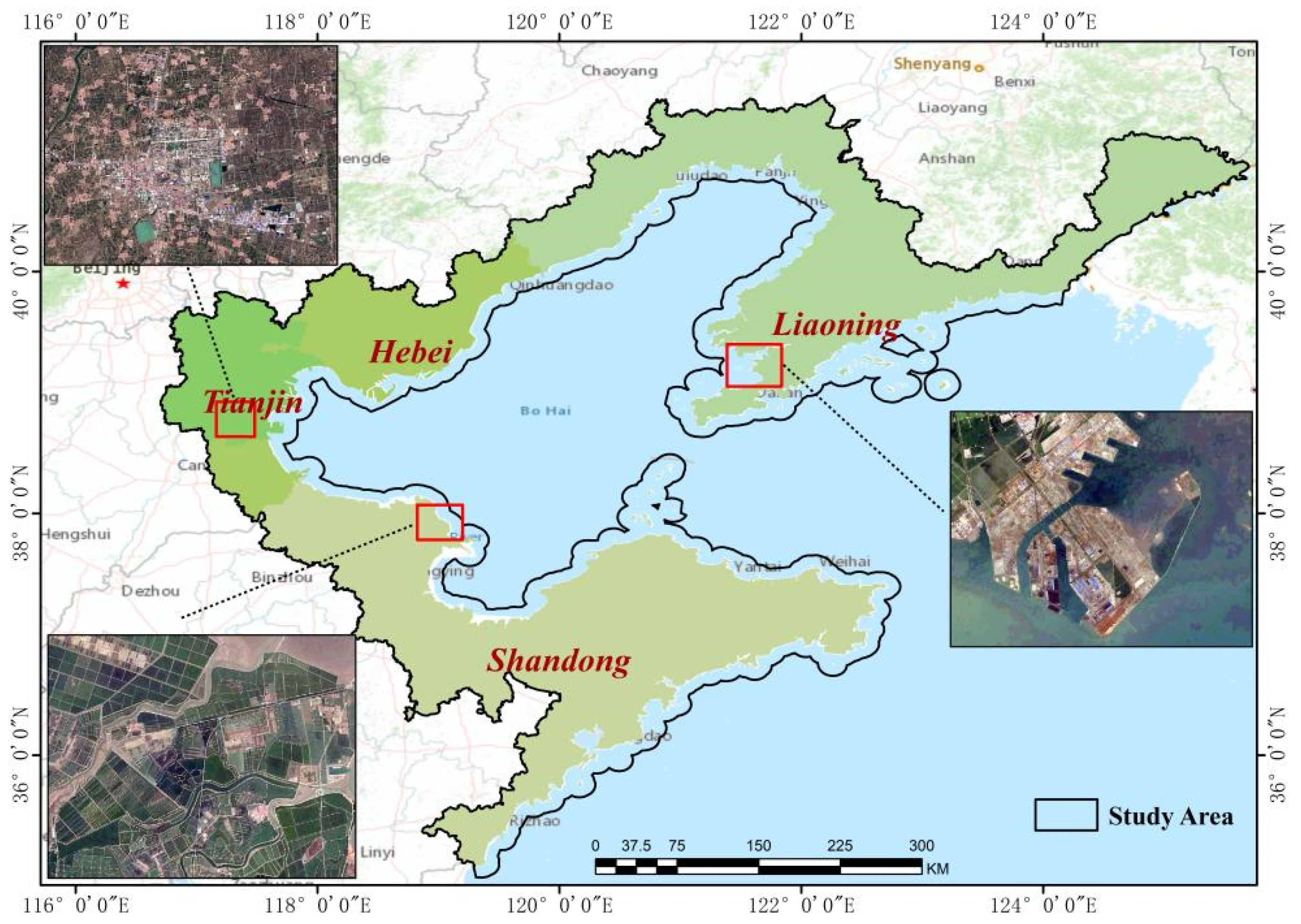
2.1. Study Area
2.2. Multi-Source Datasets
2.3. Classification System and Sampling
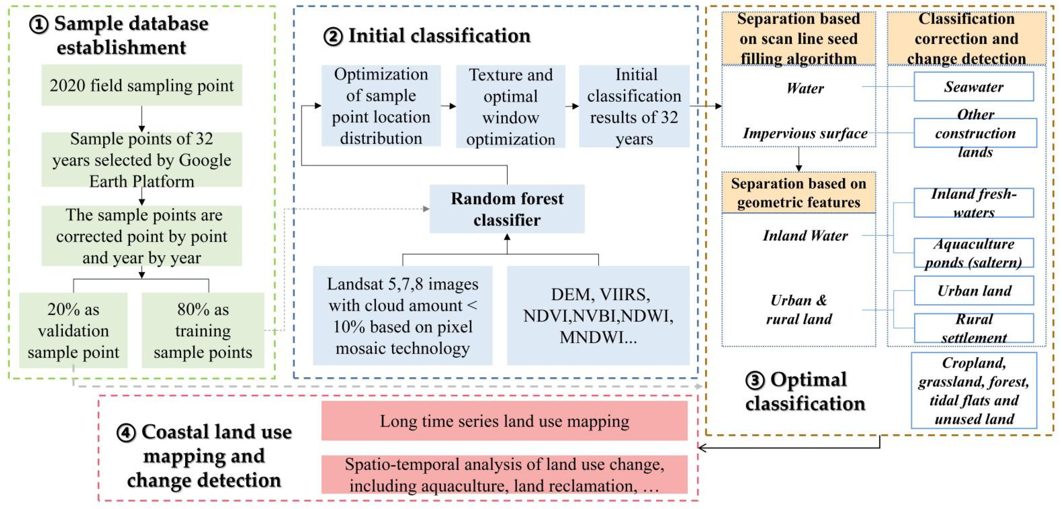
3. Methods
3.1. Initial Classification Based on Random Forest
3.2. Optimal Classification Method Based on Spatio-Temporal Logic
| Algorithm 1. The whole Algorithm is as follows, , respectively representing the output image results of different steps. |
| /* step1: Separation of impervious surface (city, rural settlement, and construction land) and water (inland fresh-waters, aquaculture ponds (saltern) and seawater) based on scan line seed */ |
| 1. |
| 2. repeat |
| 3. if then is true |
| 4. else |
| 5. |
| 6. Until stack is null |
| /* step2: Separation of inland fresh-waters and aquaculture ponds (saltern) based on spatial morphology */ |
| 7. if |
| 8. |
| 9. the 8-connectivity neighborhood outlines |
| 10. |
| 11. ,, |
| 12. if then is true |
| /* bi-directional spatio-temporal logical consistency check */ |
| 13. |
| 14. |
| 15. If and , then |
| 16. If and , then |
| 17. End |
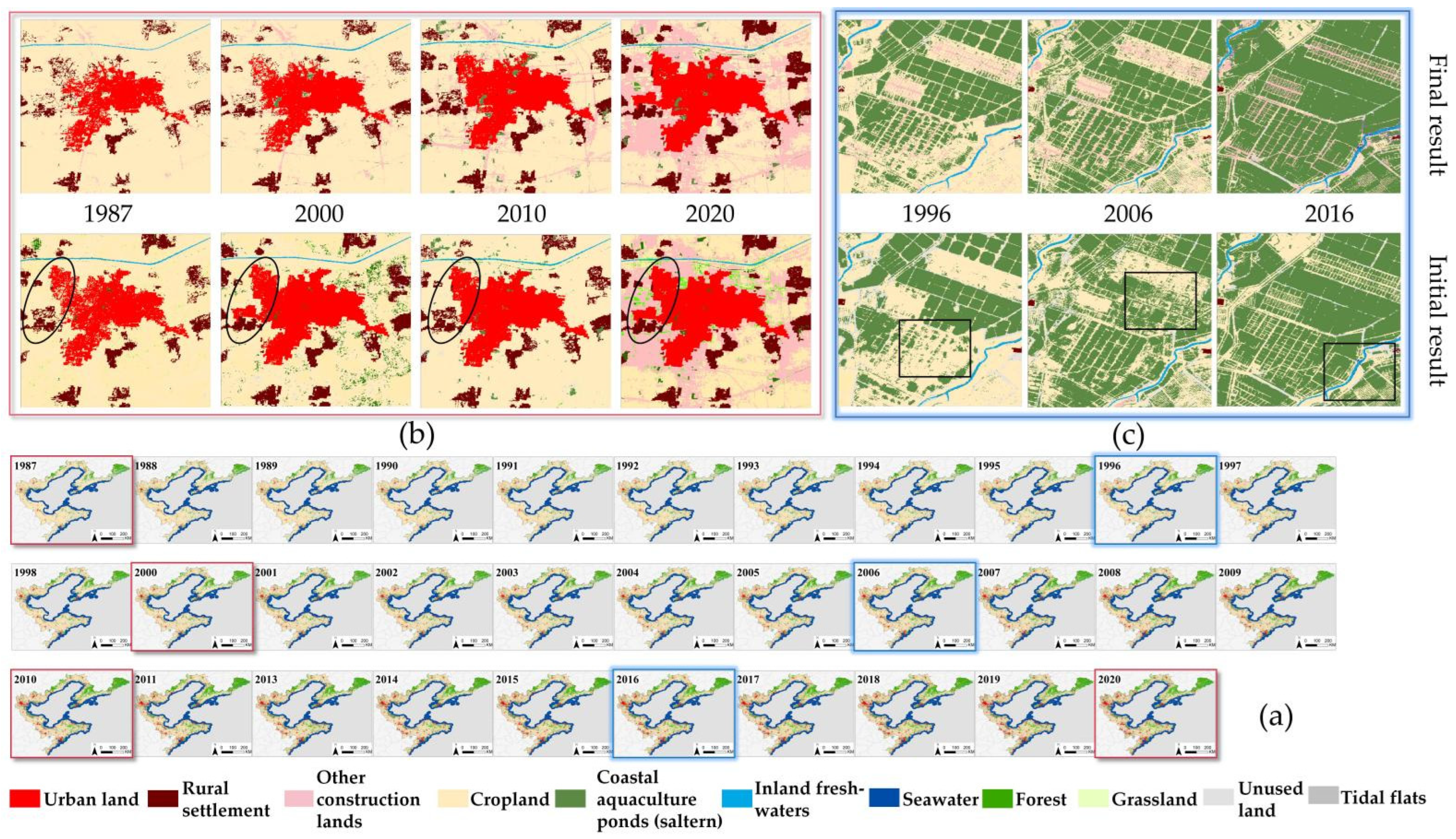
4. Results
4.1. Land Use Classification and Accuracy
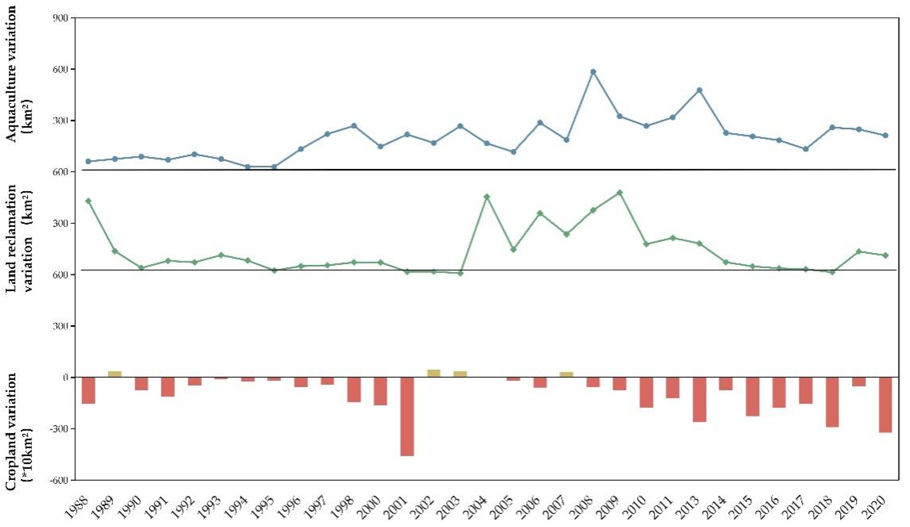
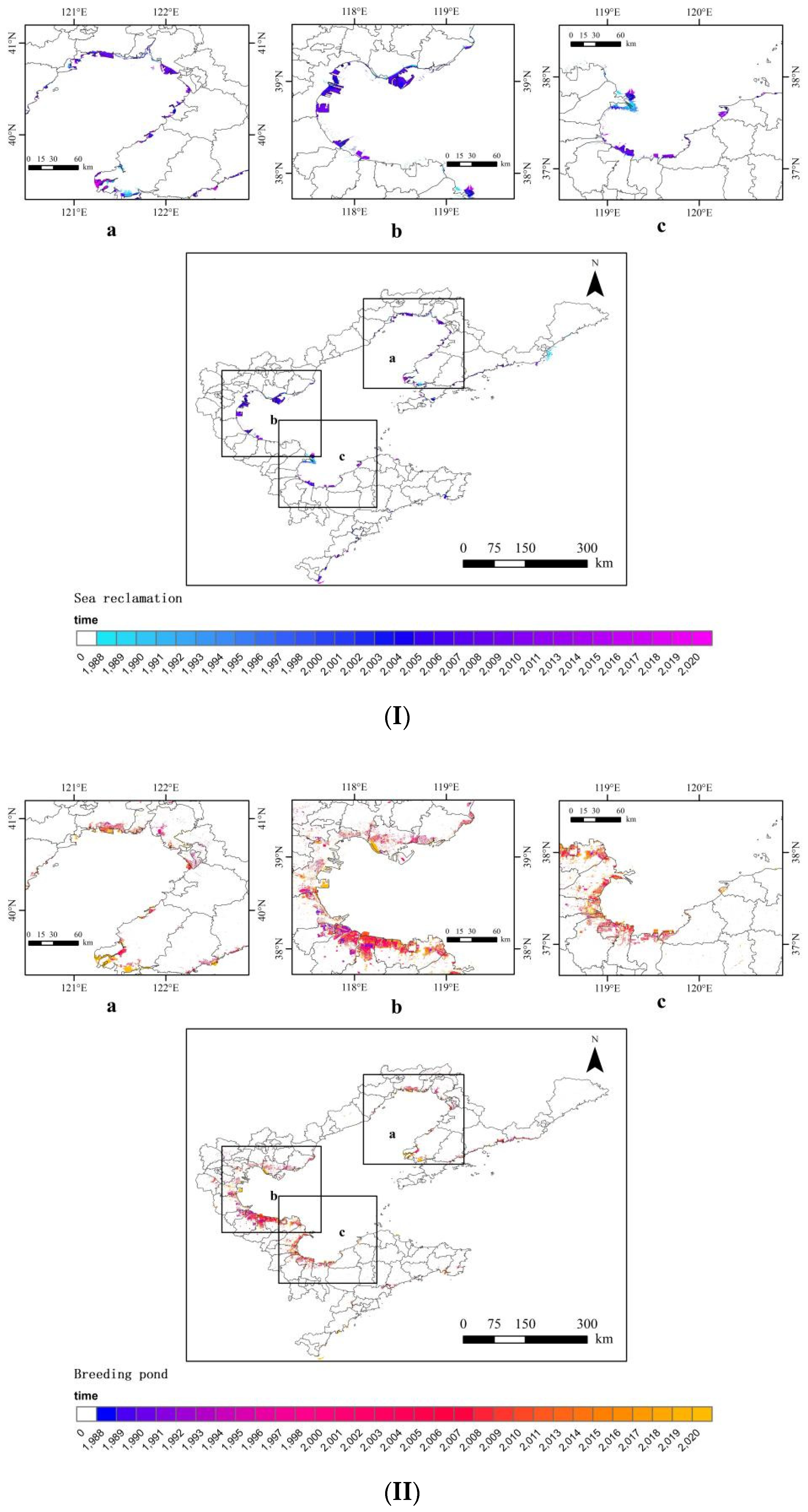
4.2. Land Reclamation and Aquaculture Changes
5. Discussion
6. Conclusions
Author Contributions
Funding
Acknowledgments
Conflicts of Interest
References
- Chuai, X.; Wen, J.; Zhuang, D.; Guo, X.; Yuan, Y.; Lu, Y.; Zhang, M.; Li, J. Intersection of Physical and Anthropogenic Effects on Land-Use/Land-Cover Changes in Coastal China of Jiangsu Province. Sustainability 2019, 11, 2370. [Google Scholar] [CrossRef] [Green Version]
- Tian, B.; Wu, W.; Yang, Z.; Zhou, Y. Drivers, trends, and potential impacts of long-term coastal reclamation in China from 1985 to 2010. Estuarine Coast. Shelf Sci. 2016, 170, 83–90. [Google Scholar] [CrossRef]
- Wang, D.; Chen, W.; Wei, W.; Bird, B.W.; Zhang, L.; Sang, M.; Wang, Q. Research on the Relationship between Urban Development Intensity and Eco-Environmental Stresses in Bohai Rim Coastal Area, China. Sustainability 2016, 8, 406. [Google Scholar] [CrossRef] [Green Version]
- Zong, S.; Hu, Y.; Zhang, Y.; Wang, W. Identification of land use conflicts in China’s coastal zones: From the perspective of ecological security. Ocean Coast. Manag. 2021, 213, 105841. [Google Scholar] [CrossRef]
- Zou, L.; Liu, Y.; Wang, J.; Yang, Y.; Wang, Y. Land use conflict identification and sustainable development scenario simulation on China’s southeast coast. J. Clean. Prod. 2019, 238, 117899. [Google Scholar] [CrossRef]
- Yasir, M.; Hui, S.; Binghu, H.; Rahman, S.U. Coastline extraction and land use change analysis using remote sensing (RS) and geographic information system (GIS) technology—A review of the literature. Rev. Environ. Health 2020, 35, 453–460. [Google Scholar] [CrossRef]
- Camilleri, S.; De Giglio, M.; Stecchi, F.; Pérez-Hurtado, A. Land use and land cover change analysis in predominantly man-made coastal wetlands: Towards a methodological framework. Wetl. Ecol. Manag. 2017, 25, 23–43. [Google Scholar] [CrossRef]
- Liu, C.; Yang, M.; Hou, Y.; Xue, X. Ecosystem service multifunctionality assessment and coupling coordination analysis with land use and land cover change in China’s coastal zones. Sci. Total Environ. 2021, 797, 149033. [Google Scholar] [CrossRef] [PubMed]
- Tian, Y.; Zhou, D.; Jiang, G. Conflict or Coordination? Multiscale assessment of the spatio-temporal coupling relationship between urbanization and ecosystem services: The case of the Jingjinji Region, China. Ecol. Indic. 2020, 117, 106543. [Google Scholar] [CrossRef]
- Coppin, P.R.; Bauer, M.E. Digital change detection in forest ecosystems with remote sensing imagery. Remote Sens. Rev. 1996, 13, 207–234. [Google Scholar] [CrossRef]
- Mountrakis, G.; Im, J.; Ogole, C. Support vector machines in remote sensing: A review. ISPRS J. Photogramm. Remote Sens. 2011, 66, 247–259. [Google Scholar] [CrossRef]
- Schneider, A. Monitoring land cover change in urban and peri-urban areas using dense time stacks of Landsat satellite data and a data mining approach. Remote Sens. Environ. 2012, 124, 689–704. [Google Scholar] [CrossRef]
- Xie, S.; Liu, L.; Zhang, X.; Yang, J.; Chen, X.; Gao, Y. Automatic Land-Cover Mapping using Landsat Time-Series Data based on Google Earth Engine. Remote Sens. 2019, 11, 3023. [Google Scholar] [CrossRef] [Green Version]
- Vali, A.; Comai, S.; Matteucci, M. Deep Learning for Land Use and Land Cover Classification based on Hyperspectral and Multispectral Earth Observation Data: A Review. Remote Sens. 2020, 12, 2495. [Google Scholar] [CrossRef]
- Jin, Y.; Liu, X.; Yao, J.; Zhang, X.; Zhang, H. Mapping the annual dynamics of cultivated land in typical area of the Middle-lower Yangtze plain using long time-series of Landsat images based on Google Earth Engine. Int. J. Remote Sens. 2019, 41, 1625–1644. [Google Scholar] [CrossRef]
- Grings, F.; Roitberg, E.; Barraza, V. EVI Time-Series Breakpoint Detection Using Convolutional Networks for Online Deforestation Monitoring in Chaco Forest. IEEE Trans. Geosci. Remote Sens. 2019, 58, 1303–1312. [Google Scholar] [CrossRef]
- Verbesselt, J.; Hyndman, R.; Newnham, G.; Culvenor, D. Detecting trend and seasonal changes in satellite image time series. Remote Sens. Environ. 2010, 114, 106–115. [Google Scholar] [CrossRef]
- Yang, Z.; Li, J.; Shen, Y.; Miao, H.; Yan, X. A denoising method for inter-annual NDVI time series derived from Landsat images. Int. J. Remote Sens. 2018, 39, 3816–3827. [Google Scholar] [CrossRef]
- Gorelick, N.; Hancher, M.; Dixon, M.; Ilyushchenko, S.; Thau, D.; Moore, R. Google Earth Engine: Planetary-scale geospatial analysis for everyone. Remote Sens. Environ. 2017, 202, 18–27. [Google Scholar] [CrossRef]
- Wang, X.; Xiao, X.; Zou, Z.; Chen, B.; Ma, J.; Dong, J.; Doughty, R.B.; Zhong, Q.; Qin, Y.; Dai, S.; et al. Tracking annual changes of coastal tidal flats in China during 1986–2016 through analyses of Landsat images with Google Earth Engine. Remote Sens. Environ. 2020, 238, 110987. [Google Scholar] [CrossRef] [PubMed]
- Zhang, K.; Dong, X.; Liu, Z.; Gao, W.; Hu, Z.; Wu, G. Mapping Tidal Flats with Landsat 8 Images and Google Earth Engine: A Case Study of the China’s Eastern Coastal Zone circa 2015. Remote Sens. 2019, 11, 924. [Google Scholar] [CrossRef] [Green Version]
- Badamfirooz, J.; Mousazadeh, R. Quantitative assessment of land use/land cover changes on the value of ecosystem services in the coastal landscape of Anzali International Wetland. Environ. Monit. Assess. 2019, 191, 694. [Google Scholar] [CrossRef]
- Gao, Y.; Cui, L.; Liu, J.; Li, W.; Lei, Y. China’s coastal-wetland change analysis based on high-resolution remote sensing. Mar. Freshw. Res. 2020, 71, 1161–1181. [Google Scholar] [CrossRef]
- Veettil, B.K.; Quang, N.X. Mangrove forests of Cambodia: Recent changes and future threats. Ocean Coast. Manag. 2019, 181, 181. [Google Scholar] [CrossRef]
- Ma, C.; Ai, B.; Zhao, J.; Xu, X.; Huang, W. Change Detection of Mangrove Forests in Coastal Guangdong during the Past Three Decades Based on Remote Sensing Data. Remote Sens. 2019, 11, 921. [Google Scholar] [CrossRef] [Green Version]
- Fu, Y.; Guo, Q.; Wu, X.; Fang, H.; Pan, Y. Analysis and Prediction of Changes in Coastline Morphology in the Bohai Sea, China, Using Remote Sensing. Sustainability 2017, 9, 900. [Google Scholar] [CrossRef] [Green Version]
- Wang, Y.; Hou, X.; Shi, P.; Yu, L. Detecting Shoreline Changes in Typical Coastal Wetlands of Bohai Rim in North China. Wetlands 2013, 33, 617–629. [Google Scholar] [CrossRef]
- Xu, N.; Gao, Z.; Ning, J. Analysis of the characteristics and causes of coastline variation in the Bohai Rim (1980–2010). Environ. Earth Sci. 2016, 75, 1–11. [Google Scholar] [CrossRef]
- Fu, Y.; Deng, J.; Wang, H.; Comber, A.; Yang, W.; Wu, W.; You, S.; Lin, Y.; Wang, K. A new satellite-derived dataset for marine aquaculture areas in China’s coastal region. Earth Syst. Sci. Data 2021, 13, 1829–1842. [Google Scholar] [CrossRef]
- Duan, Y.; Li, X.; Zhang, L.; Liu, W.; Liu, S.; Chen, D.; Ji, H. Detecting spatiotemporal changes of large-scale aquaculture ponds regions over 1988–2018 in Jiangsu Province, China using Google Earth Engine. Ocean Coast. Manag. 2020, 188, 105144. [Google Scholar] [CrossRef]
- Sun, S.; Zhang, Y.; Song, Z.; Chen, B.; Zhang, Y.; Yuan, W.; Chen, C.; Chen, W.; Ran, X.; Wang, Y. Mapping Coastal Wetlands of the Bohai Rim at a Spatial Resolution of 10 m Using Multiple Open-Access Satellite Data and Terrain Indices. Remote Sens. 2020, 12, 4114. [Google Scholar] [CrossRef]
- Xia, Z.; Guo, X.; Chen, R. Automatic extraction of aquaculture ponds based on Google Earth Engine. Ocean Coast. Manag. 2020, 198, 105348. [Google Scholar] [CrossRef]
- Huang, C.; Zhang, C.; Liu, Q.; Wang, Z.; Li, H.; Liu, G. Land reclamation and risk assessment in the coastal zone of China from 2000 to 2010. Reg. Stud. Mar. Sci. 2020, 39, 101422. [Google Scholar] [CrossRef]
- Sengupta, D.; Chen, R.; Meadows, M.E.; Choi, Y.R.; Banerjee, A.; Zilong, X. Mapping Trajectories of Coastal Land Reclamation in Nine Deltaic Megacities using Google Earth Engine. Remote Sens. 2019, 11, 2621. [Google Scholar] [CrossRef] [Green Version]
- Chen, J.; Chen, J.; Liao, A.; Cao, X.; Chen, L.; Chen, X.; He, C.; Han, G.; Peng, S.; Lu, M.; et al. Global land cover mapping at 30 m resolution: A POK-based operational approach. ISPRS J. Photogramm. Remote Sens. 2015, 103, 7–27. [Google Scholar] [CrossRef] [Green Version]
- Gong, P.; Wang, J.; Yu, L.; Zhao, Y.; Zhao, Y.; Liang, L.; Niu, Z.; Huang, X.; Fu, H.; Liu, S.; et al. Finer resolution observation and monitoring of global land cover: First mapping results with Landsat TM and ETM+ data. Int. J. Remote Sens. 2012, 34, 2607–2654. [Google Scholar] [CrossRef] [Green Version]
- Sun, Z.; Luo, J.; Yang, J.; Yu, Q.; Zhang, L.; Xue, K.; Lu, L. Nation-Scale Mapping of Coastal Aquaculture Ponds with Sentinel-1 SAR Data Using Google Earth Engine. Remote Sens. 2020, 12, 3086. [Google Scholar] [CrossRef]
- Virdis, S.G.P. An object-based image analysis approach for aquaculture ponds precise mapping and monitoring: A case study of Tam Giang-Cau Hai Lagoon, Vietnam. Environ. Monit. Assess. 2014, 186, 117–133. [Google Scholar] [CrossRef]
- Cheng, B.; Liang, C.; Liu, X.; Liu, Y.; Ma, X.; Wang, G. Research on a novel extraction method using Deep Learning based on GF-2 images for aquaculture areas. Int. J. Remote Sens. 2020, 41, 3575–3591. [Google Scholar] [CrossRef]
- Han, X.; Chen, X.; Feng, L. Four decades of winter wetland changes in Poyang Lake based on Landsat observations between 1973 and 2013. Remote Sens. Environ. 2015, 156, 426–437. [Google Scholar] [CrossRef]
- Sheng, Y.; Song, C.; Wang, J.; Lyons, E.; Knox, B.R.; Cox, J.S.; Gao, F. Representative lake water extent mapping at continental scales using multi-temporal Landsat-8 imagery. Remote Sens. Environ. 2016, 185, 129–141. [Google Scholar] [CrossRef] [Green Version]
- Liu, Y.; Hou, X.; Li, X.; Song, B.; Wang, C. Assessing and predicting changes in ecosystem service values based on land use/cover change in the Bohai Rim coastal zone. Ecol. Indic. 2020, 111, 106004. [Google Scholar] [CrossRef]
- Zhang, Y.; Zhao, L.; Liu, J.; Liu, Y.; Li, C. The Impact of Land Cover Change on Ecosystem Service Values in Urban Agglomerations along the Coast of the Bohai Rim, China. Sustainability 2015, 7, 10365–10387. [Google Scholar] [CrossRef] [Green Version]
- Ding, Z.; Su, F.; Zhang, J.; Zhang, Y.; Luo, S.; Tang, X. Clustering Coastal Land Use Sequence Patterns along the Sea–Land Direction: A Case Study in the Coastal Zone of Bohai Bay and the Yellow River Delta, China. Remote Sens. 2019, 11, 2024. [Google Scholar] [CrossRef] [Green Version]
- Li, H.; Wan, W.; Fang, Y.; Zhu, S.; Chen, X.; Liu, B.; Hong, Y. A Google Earth Engine-enabled software for efficiently generating high-quality user-ready Landsat mosaic images. Environ. Model. Softw. 2019, 112, 16–22. [Google Scholar] [CrossRef]
- Jiang, H.; Feng, M.; Zhu, Y.; Lu, N.; Huang, J.; Xiao, T. An Automated Method for Extracting Rivers and Lakes from Landsat Imagery. Remote Sens. 2014, 6, 5067–5089. [Google Scholar] [CrossRef] [Green Version]
- Zeng, Z.; Wang, D.; Tan, W.; Huang, J. Extracting aquaculture ponds from natural water surfaces around inland lakes on medium resolution multispectral images. Int. J. Appl. Earth Obs. Geoinf. 2019, 80, 13–25. [Google Scholar] [CrossRef]
- Heydari, S.S.; Mountrakis, G. Effect of classifier selection, reference sample size, reference class distribution and scene heterogeneity in per-pixel classification accuracy using 26 Landsat sites. Remote Sens. Environ. 2018, 204, 648–658. [Google Scholar] [CrossRef]
- Feyisa, G.L.; Meilby, H.; Fensholt, R.; Proud, S.R. Automated Water Extraction Index: A new technique for surface water mapping using Landsat imagery. Remote Sens. Environ. 2014, 140, 23–35. [Google Scholar] [CrossRef]
- Zhou, Y.; Dong, J.; Xiao, X.; Xiao, T.; Yang, Z.; Zhao, G.; Zou, Z.; Qin, Y. Open Surface Water Mapping Algorithms: A Comparison of Water-Related Spectral Indices and Sensors. Water 2017, 9, 256. [Google Scholar] [CrossRef]
- Van Der Werff, H.; Van Der Meer, F. Shape-based classification of spectrally identical objects. ISPRS J. Photogramm. Remote Sens. 2008, 63, 251–258. [Google Scholar] [CrossRef]
- Li, X.; Gong, P.; Liang, L. A 30-year (1984–2013) record of annual urban dynamics of Beijing City derived from Landsat data. Remote Sens. Environ. 2015, 166, 78–90. [Google Scholar] [CrossRef]
- Wang, X.; Xiao, X.; Zou, Z.; Hou, L.; Qin, Y.; Dong, J.; Doughty, R.B.; Chen, B.; Zhang, X.; Chen, Y.; et al. Mapping coastal wetlands of China using time series Landsat images in 2018 and Google Earth Engine. ISPRS J. Photogramm. Remote Sens. 2020, 163, 312–326. [Google Scholar] [CrossRef] [PubMed]
- Kim, H.; Lee, S.B.; Min, K.S. Shoreline Change Analysis using Airborne LiDAR Bathymetry for Coastal Monitoring. J. Coast. Res. 2017, 79, 269–273. [Google Scholar] [CrossRef] [Green Version]
- Ottinger, M.; Clauss, K.; Kuenzer, C. Aquaculture: Relevance, distribution, impacts and spatial assessments—A review. Ocean Coast. Manag. 2016, 119, 244–266. [Google Scholar] [CrossRef]


| Class I | Class II | Description |
|---|---|---|
| Cropland | - | Refers to land used for growing crops |
| Grassland | - | Natural grassland and improved grassland |
| Forest | - | Refers to natural and man-made forests with canopy density >30% |
| Water | Coastal aquaculture ponds (saltern) | Shallow artificial water bodies with distinctly man-made shape for aquaculture production |
| Seawater | Shallow sea within 10 km offshore buffer zone | |
| Inland fresh-waters | Rivers, ditches, reservoirs, lakes, and other natural water bodies | |
| Impervious surface | Urban land | Land for urban and built-up areas above county level |
| Rural settlement | Residential land below county level | |
| Other construction lands | Independent of factories and mines, large industrial areas, ports, transportation land, airports, and special land outside cities and towns | |
| Other land | Tidal flats | Beaches, salt marshes, and bare land in coastal areas |
| Unused land | Land not yet used, including barren land |
| 2020 | CRP | GRS | FRT | APS | UBL | UUS | IFW | TDF | RST | CIT | SWT | |
|---|---|---|---|---|---|---|---|---|---|---|---|---|
| 1987 | ||||||||||||
| CRP | 66.59 | 2.28 | 5.07 | 4.72 | 9.46 | 0.80 | 0.56 | 0.25 | 6.49 | 3.25 | 0.52 | |
| GRS | 16.02 | 36.60 | 43.08 | 0.27 | 1.04 | 1.47 | 0.10 | 0.14 | 0.63 | 0.65 | 0.00 | |
| FRT | 1.11 | 7.28 | 90.47 | 0.09 | 0.15 | 0.62 | 0.01 | 0.06 | 0.07 | 0.13 | 0.00 | |
| APS | 22.37 | 1.20 | 6.40 | 43.80 | 16.80 | 0.92 | 0.51 | 0.39 | 2.21 | 4.27 | 1.13 | |
| UBL | 0.00 | 0.00 | 0.00 | 0.00 | 100.00 | 0.00 | 0.00 | 0.00 | 0.00 | 0.00 | 0.00 | |
| UUS | 8.06 | 34.84 | 50.05 | 0.51 | 0.64 | 4.07 | 0.56 | 0.00 | 0.64 | 0.61 | 0.02 | |
| IFW | 3.99 | 0.22 | 2.63 | 0.70 | 1.51 | 0.55 | 88.37 | 0.01 | 0.32 | 0.38 | 1.32 | |
| TDF | 4.26 | 19.72 | 40.93 | 1.30 | 5.03 | 0.00 | 0.07 | 20.72 | 2.50 | 3.86 | 1.60 | |
| RST | 0.00 | 0.00 | 0.00 | 0.00 | 0.00 | 0.00 | 0.00 | 0.00 | 78.78 | 21.22 | 0.00 | |
| CIT | 0.00 | 0.00 | 0.00 | 0.00 | 0.00 | 0.00 | 0.00 | 0.00 | 0.00 | 99.99 | 0.01 | |
| SWT | 0.84 | 0.04 | 0.09 | 2.59 | 2.60 | 0.00 | 0.02 | 0.51 | 0.06 | 0.27 | 92.96 | |
Publisher’s Note: MDPI stays neutral with regard to jurisdictional claims in published maps and institutional affiliations. |
© 2021 by the authors. Licensee MDPI, Basel, Switzerland. This article is an open access article distributed under the terms and conditions of the Creative Commons Attribution (CC BY) license (https://creativecommons.org/licenses/by/4.0/).
Share and Cite
Chen, D.; Wang, Y.; Shen, Z.; Liao, J.; Chen, J.; Sun, S. Long Time-Series Mapping and Change Detection of Coastal Zone Land Use Based on Google Earth Engine and Multi-Source Data Fusion. Remote Sens. 2022, 14, 1. https://0-doi-org.brum.beds.ac.uk/10.3390/rs14010001
Chen D, Wang Y, Shen Z, Liao J, Chen J, Sun S. Long Time-Series Mapping and Change Detection of Coastal Zone Land Use Based on Google Earth Engine and Multi-Source Data Fusion. Remote Sensing. 2022; 14(1):1. https://0-doi-org.brum.beds.ac.uk/10.3390/rs14010001
Chicago/Turabian StyleChen, Dong, Yafei Wang, Zhenyu Shen, Jinfeng Liao, Jiezhi Chen, and Shaobo Sun. 2022. "Long Time-Series Mapping and Change Detection of Coastal Zone Land Use Based on Google Earth Engine and Multi-Source Data Fusion" Remote Sensing 14, no. 1: 1. https://0-doi-org.brum.beds.ac.uk/10.3390/rs14010001