Article

Using Remote Sensing and Machine Learning to Locate Groundwater Discharge to Salmon-Bearing Streams

1
School of Geosciences, University of South Florida, Tampa, FL 33620, USA
2
Land Resources and Environmental Sciences, Montana State University, Bozeman, MT 59717, USA
*
Author to whom correspondence should be addressed.
Submission received: 9 October 2021 / Revised: 18 December 2021 / Accepted: 23 December 2021 / Published: 24 December 2021
(This article belongs to the Special Issue Remote Sensing of Fluvial Systems)

Abstract

:
We hypothesized topographic features alone could be used to locate groundwater discharge, but only where diagnostic topographic signatures could first be identified through the use of limited field observations and geologic data. We built a geodatabase from geologic and topographic data, with the geologic data only covering ~40% of the study area and topographic data derived from airborne LiDAR covering the entire study area. We identified two types of groundwater discharge: shallow hillslope groundwater discharge, commonly manifested as diffuse seeps, and aquifer-outcrop groundwater discharge, commonly manifested as springs. We developed multistep manual procedures that allowed us to accurately predict the locations of both types of groundwater discharge in 93% of cases, though only where geologic data were available. However, field verification suggested that both types of groundwater discharge could be identified by specific combinations of topographic variables alone. We then applied maximum entropy modeling, a machine learning technique, to predict the prevalence of both types of groundwater discharge using six topographic variables: profile curvature range, with a permutation importance of 43.2%, followed by distance to flowlines, elevation, topographic roughness index, flow-weighted slope, and planform curvature, with permutation importance of 20.8%, 18.5%, 15.2%, 1.8%, and 0.5%, respectively. The AUC values for the model were 0.95 for training data and 0.91 for testing data, indicating outstanding model performance.

1. Introduction

Many ecosystems depend on groundwater discharge, including many wetlands [1,2], lakes [3,4], streams [5,6], and estuaries [7,8]. Groundwater discharge to streams is particularly prevalent and critical, being the sole source of baseflow by definition [9] and commonly a substantive subcomponent of stormflow [10]. Though regionally variable, estimates suggest that groundwater discharge provides 14–90% of all stream flow in the conterminous United States [5]. In addition to subsidizing stream flow, groundwater discharge to streams can also modulate stream temperature [11,12] and deliver nutrients and organic carbon [13,14], thereby playing important roles in structuring habitats from the benthos [15] to the fish [16]. Groundwater is also an important water supply component, with 321,000,000 m3 of groundwater withdrawals comprising 26% of all water use in the United States in 2015 [17]. Many of these withdrawals are centralized, including withdrawals for thermoelectric power generation (41%), public water supply (12%), and industrial water supply (5%). Others are more dispersed, including irrigation water supply (37%) and domestic water supply (1%). Effective management and protection of groundwater resources is critical, therefore, to a diverse suite of natural and human users [18].
The first step toward protecting groundwater discharge to ecosystems is to determine the types of groundwater discharge (e.g., sourced from local versus regional groundwater flow systems), the locations where groundwater discharge occurs, and their support for downgradient ecosystems (e.g., fluvial ecosystems). Field studies are often essential in identifying types and locations of groundwater discharge, especially in geologically complex regions where there may be more than one type of groundwater discharge from more than one type of geologic unit [19,20]. Field mapping of these types of groundwater discharge is possible in some situations (e.g., [21]) but is impractical over large spatial scales and/or in difficult-to-access regions. In these instances, remote sensing, geospatial modeling, and/or machine learning have been used to map remote locations where groundwater discharge occurs, with some degree of success (e.g., [22,23]). These tools are receiving increased attention for general applications in hydrology as computer processing power increases and remote sensing data become more easily available.
The ways remote sensing, geospatial modeling, and/or machine learning are used in hydrologic studies depends on the question being addressed; the spatial and temporal scale of the question; and the type, amount, and quality of the available data [24,25,26]. Nevertheless, these tools have been incorporated into strategies to forecast groundwater levels [27,28,29,30], groundwater quality [31,32,33], saltwater intrusion and groundwater salinity [34], and groundwater resource availability [35,36]. Using these approaches to better understand and predict groundwater discharge is particularly challenging (e.g., [22,23]). In many cases, groundwater discharge occurs where erosion or tectonic uplift has exposed aquifers, creating aquifer outcrops. This means that better understanding and predicting groundwater discharge requires an understanding of both topography and geology, with subsurface lithology commonly being poorly known [22,23] yet nevertheless playing a disproportionately important role [30].
The primary controls on groundwater recharge, flow, and discharge are climate, geology, and topography [37]. Climate is typically constant across large study areas, and regional-scale geologic data are difficult to obtain, so studies typically rely upon topography to characterize generalized hydrology [38,39] and locations where groundwater discharge is likely to occur [23,40,41]. However, geologic heterogeneity often plays a controlling role in groundwater recharge, flow, and discharge [42], leading some to suggest that geologic data are more important than topographic data when characterizing hydrological processes (e.g., [30,43]). However, accurate prediction of groundwater discharge is often desired in regions where the geology is heterogeneous and anisotropic, poorly understood, and/or inadequately documented. We therefore hypothesized that topographic features alone could be used to locate groundwater discharge, but only where diagnostic topographic signatures could first be identified through field observations and geologic data covering a characteristic subset of the study area. We based this hypothesis on the understanding that groundwater levels and discharges play important roles in structuring local- and watershed-scale geomorphology, thereby affecting topography [44,45], and that groundwater flow systems are typically attracted to the land surface at concave surfaces, such as hillslope failures and toeslopes [2,46,47]. We tested this hypothesis in south-central Alaska, in a large area that is difficult to access and where geologic data are incompletely available but where remotely sensed LiDAR-based topographic data are widely available.

2. Materials and Methods

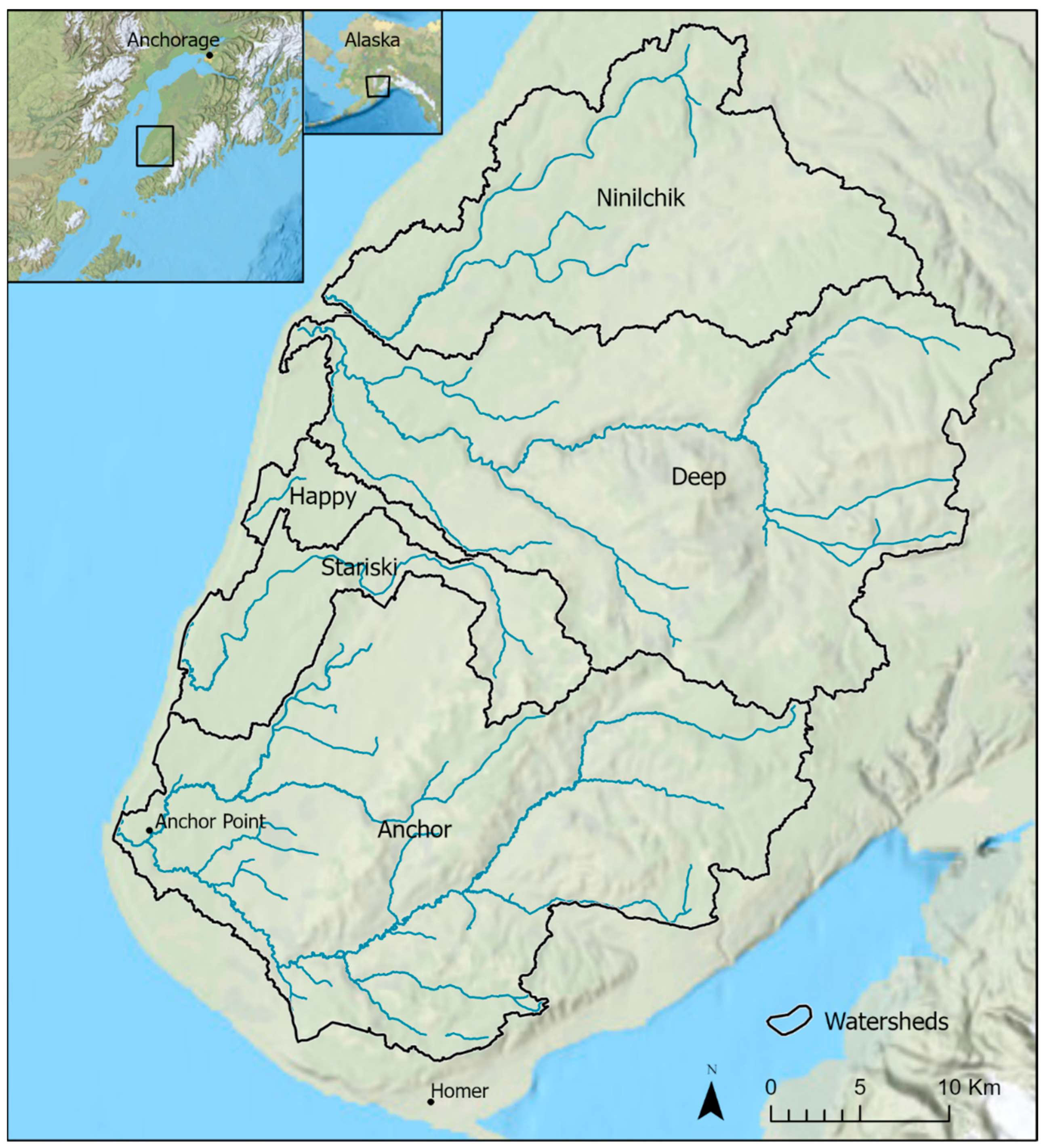
2.1. Site Description

The study was conducted on the Kenai Peninsula Lowlands in south-central Alaska (Figure 1). The study area is a 1655 km2 area comprising five watersheds: Anchor River, Stariski Creek, Happy Creek, Deep Creek, and the Ninilchik River, from south to north respectively. All except Happy Creek are salmon-bearing and therefore support vibrant sport and commercial fisheries that are central to the regional economy [48,49]. Groundwater discharge plays a critical role in controlling the structure and function of these streams, by augmenting stream flow, modulating stream temperatures, and delivering nutrient subsidies [12,14]. Most of the study area is roadless or accessible only by unimproved roads. However, more than 80% of the land is privately owned and has begun seeing steadily increasing development pressure [50], particularly in the western region of the study area and primarily to support single-family homes and farm-to-fork agriculture [51]. Groundwater is the primary source of water for domestic, commercial, and industrial uses [52] and is also threatened by land-use/land-cover change [53], aggregate mining [49], and a drying trend in the climate [54,55,56].
The climate is transitional from maritime to coastal and consists of short summers and long winters (HOMER 8 NW, ALASKA [503672], 1981–2010). The mean annual minimum temperature is −0.8 °C, and the mean annual maximum temperature is 6.1 °C. Total annual precipitation is 748 mm, with approximately one-third falling as snow and approximately half falling during the wet season (i.e., August–November). The study area underwent at least five major Pleistocene glaciations and two minor post-Pleistocene glacial advances, each variously recorded in ice-scoured landforms, drift sheets, moraines, and discordant drainage relations separated by unconformities and weathering profiles [58]. Most of the study region is now covered with younger glacial outwash and valley train; glaciolacustrine; and other minor terminal, recessional, lateral, medial, and ground moraine deposits [59], some reworked by the recent minor glacial advances. Groundwater is found in both surficial deposits, often in wetlands, and in deeper deposits, commonly in thin, discontinuous, and poorly lithified sandstone aquifers formed in buried channel lag and bar deposits [60]. Overall topographic relief ranges from 0 to 889 m above mean sea level (AMSL). Local topography is also commonly steep, as streams have deeply dissected the landscape during the Quaternary.

2.2. Overall Approach

The study proceeded in three phases. During the first phase, we created a geographic information system (GIS) geodatabase from geologic and topographic data. Geologic data were sourced from publicly available well logs available for ~40% of the study area; topographic data were sourced from airborne LiDAR available for the entire study area. During the second phase, we stayed within the subset of the study area where geological data were available, using the geodatabase and field observations to identify two types of groundwater discharge and locations where they occurred. The geologic data and geodatabase were essential to the initial identification of one of those two types of groundwater discharge and locations where it occurred. However, field observations suggested that these locations could also be identified by specific combinations of topographic variables alone even where geologic data were not available (e.g., numerous narrow gullies and other deeply incised headwater stream channels that abruptly start along the same topographic contour interval on a hillslope). In the final phase, we used a machine learning approach using only topographic data to predict the likelihood that either type of groundwater discharge occurs.

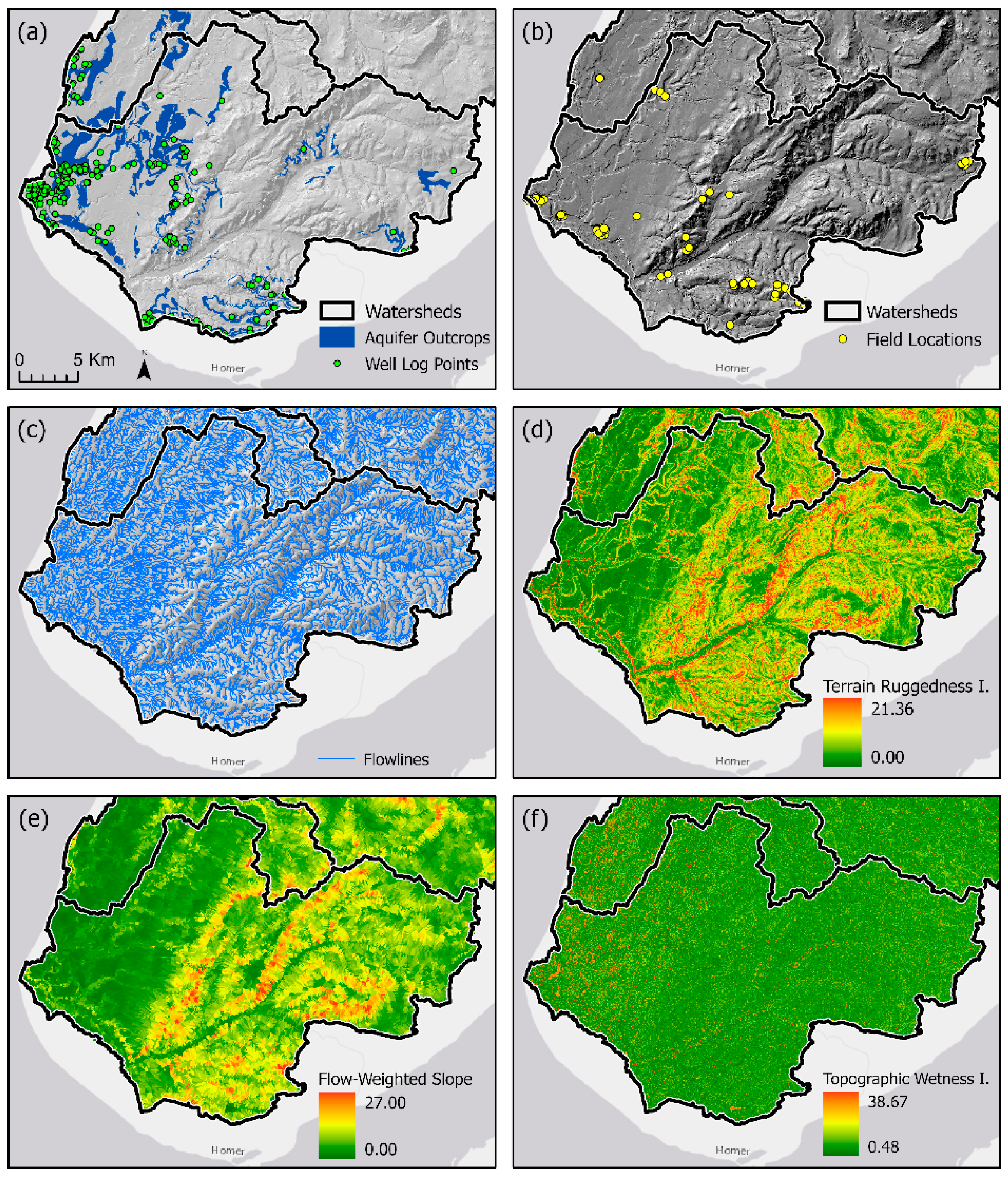
2.3. Geodatabase Development

2.3.1. Geologic Data

Subsurface geologic data were obtained from well logs in the publicly available Well Log Tracking System (WELTS) maintained by the Alaska Department of Natural Resources (https://dnr.alaska.gov/welts/; accessed on 29 May 2019). Records from >800 well logs within and immediately adjacent to the study area were used to quantify the locations, depths, thicknesses, and geologic characteristics of the water-bearing formations, i.e., the aquifers.
Depths and thicknesses of the aquifers were converted to top and bottom elevations of the aquifers. The aquifer materials are unconsolidated to poorly lithified buried channel lag and bar deposits and therefore vary slightly in thickness and slope gently in the original direction of drainage. Therefore, a user-specified 5 m vertical buffer was added to the top and subtracted from the bottom elevations of the aquifers. These vertically buffered aquifers were then projected outward from the well logs in concentric circles of increasing radii using the Inverse-Distance Weighting (IDW) interpolation tool. Areas where the buffered aquifers intersected the ground surface were found by intersecting the aquifer boundaries with a digital elevation model (DEM, see below) using the Raster Calculator tool and were mapped as potential aquifer outcrops. The final step was to determine the horizontal spatial scale over which the aquifer interpolations were valid. We did so using standard geologic mapping techniques. Geologic mapping is an interpretive method in which field observations are commonly recorded as qualitative data, such as sketches and narratives [61]. We made such qualitative observations at increasing radial distances from wells, looking for aquifer outcrops of the same material and at the same approximate elevations as described in the corresponding well log. We initially tested circles of 1000 m radius and then tested circles of 2000 and 3000 m radius as we continued to find aquifer outcrops at the outer edges of the projections, though with decreasing frequency with increasing radial distance. We then tested circles of 5000 m radius, finding no aquifer outcrops of the same material at the same approximate elevations as described in the corresponding well log. We concluded that the horizontal spatial scale over which the aquifer interpolations were valid ended somewhere between 3000 and 5000 m, and we adopted the more-conservative limit of 3000 m. This resulted in >800 overlapping circles of 3000 m radius covering ~40% of the study area, which is sufficiently representative of the entire study area. Many of these overlapping circles intersect the ground surface and therefore indicate locations where groundwater discharge from aquifer outcrops likely occurs.

2.3.2. Topographic Data

Topographic data were derived from airborne LiDAR (2008 Kenai Watershed Forum Topographic LiDAR: Kenai Peninsula, Alaska; https://www.fisheries.noaa.gov/inport/item/49620; accessed on 25 February 2019). The LiDAR-based digital elevation model (DEM) was acquired at 1 × 1 m pixel size but was resampled to a 3 × 3 m pixel size, which both reduced run times and smoothed microtopographic anomalies. The DEM was also modified to remove areas that were below the estimated tide level at the time of data collection (~3 m AMSL). This resampled and modified DEM was used to produce all topographic data using standard tools in ArcGIS 10.5 or ArcGIS Pro 2.7.1 (ESRI, Redlands, CA, USA).
Topographic data directly extracted from the DEM included elevation, slope, profile curvature, profile curvature range, planform curvature, and planform curvature range. Slope records the steepness of the terrain expressed as a percentage. Steep slopes can be indicative of steep hydraulic gradients driving shallow groundwater flow [42], and long steep slopes may be indicative of locations where aquifers might outcrop and therefore where deep groundwater discharge might occur. Profile curvature measures convexity or concavity of the slope parallel to the direction of the slope; planform curvature measures convexity or concavity of the slope perpendicular to the direction of the slope. The range of profile and planform curvatures were calculated within a 3 × 3 cell (9 × 9 m) window to measure changes in curvature over short distances, which can be an indicator of slope failures like those induced by groundwater discharge [46,47], the headward extents of channels formed by groundwater discharge [62,63], and/or locations where water tables might be close to or above the land surface [2,64].
Topographic data derived from the DEM included flowlines, terrain ruggedness index (TRI), flow-weighted slope (FWS), and topographic wetness index (TWI). Flowlines were defined by categorizing flow accumulation values higher than 2000 as streams and converting those into vector format. Flowlines may represent locations where water tables might be close to or above the land surface [6], and the headward extents of flowlines likely correlate with the headward extents of channels formed by groundwater discharge [63]. TRI measures topographic heterogeneity, calculated as the square root of the average squared differences in elevation between a pixel and its eight neighbors, and is defined per pixel as:
TRI = [ ( X i j X 00 ) 2 ] 1 2 ,
where Xij is the elevation of all eight pixels neighboring pixel X00 [65]. TRI was computed using Arc Hydro in ArcGIS Pro. TRI is an indicator of slope failures like those induced by groundwater discharge, the headward extents of channels formed by groundwater discharge, and narrow gullies and other deeply incised headwater stream channels [66]. FWS indicates the degree to which water is concentrated and then driven downslope by topography, and it is defined per subcatchment as:
FWS = ( β i F A C i ) / F A C i ,
where βi is the slope (in percent) at a particular pixel, FACi is flow accumulation for that pixel, and ∑(FACi) is the summation of flow accumulation for all pixels within the subcatchment. FWS was calculated using Arc Hydro in ArcMap 10.8. Arc Hydro was first used to calculate flow direction and flow accumulation and define, segment, and link streams. These were then used to delineate catchments using the Arc Hydro catchment grid delineation tool. The catchment grid was then converted into a polygon feature class using the Arc Hydro catchment polygon processing tool. The stream link layer was then converted into a drainage line feature class using the Arc Hydro drainage line processing tool. Finally, the Arc Hydro adjoint catchment processing tool was used to generate the aggregated upstream catchments from the catchment feature class. FWS for each catchment was then calculated from these layers using the raster calculator. FWS has been shown to correlate both with groundwater discharge [12] and stream water chemistry which itself may be a function of groundwater discharge [67]. TWI indicates where water is likely to accumulate, and it is defined per pixel as:
TWI = ln ( A Tan β 0 ) ,
where A is the area that contributes flow to a particular pixel and Tanβ0 is the tangent of the slope of the pixel being analyzed [68,69]. TWI was calculated using Arc Hydro and the TWI tool in TauDEM Version 5 (Terrain Analysis Using Digital Elevation Models; https://hydrology.usu.edu/taudem/taudem5/; accessed on 7 May 2019) in ArcMap 10.8. The D-infinity (DINF) tool in Arc Hydro was first used to calculate a slope-sensitive flow direction. The DINF is an iterative process which guarantees that each flat pixel ultimately drains to a lower elevation, eliminating the possibility of inconsistencies such as loops in the flow direction angle [70]. The DINF contributing area tool in Arc Hydro was then used to calculate a grid of pixel-specific catchment areas. TWI for each pixel was then calculated using the TWI tool from the TauDEM. TWI has also been called Wetx and Compound Topographic Index (CTI); all three utilize the same formula to represent likelihood of water flow over landscapes [68,69,71].

2.3.3. Layers Derived from the Geologic and Topographic Data

Multiple geologic and topographic layers were derived from the geologic and topographic data (Figure 2). The geologic data were obtained from >800 well logs associated with domestic, commercial, and/or industrial wells, all located proximal to roads in the more-developed western and southern parts of the study area. The topographic data were derived from a DEM which covered the entire, mostly roadless, 1655 km2 study area. Therefore, the GIS layers which represent the geologic data are situated predominantly in the western and southern portions of the study area while the layers representing the topographic data cover the full extent of the study area.

2.3.4. Field Work

Field work was conducted during the summers of 2018 and 2019. Initial field work was focused on identifying the types of groundwater discharge that occur and the conditions under which they occur. We then developed and tested procedures for the manual identification of these types of groundwater discharge using the full geologic and topographic portions of the geodatabase (i.e., both the geologic and topographic data). Using these manual procedures, we identified 67 locations in the Anchor River and Stariski Creek watersheds, the southernmost two watersheds in the study area (Figure 2). Our manual procedures predicted that groundwater discharge did occur at 54 of these locations and did not occur at 13 of these locations. We then visited each of these 67 locations, obtaining geographic positioning system (GPS) coordinates at each location with a Garmin Rino 650 handheld GPS unit (Garmin, Olathe, KS, USA) and noting if groundwater discharge actually did or did not occur. Where groundwater discharge did occur, temperature, pH, and specific conductance were measured using a YSI MPS 556 (YSI, Yellow Springs, OH, USA). Specific conductance was particularly important because it is a proxy for water–rock contact time, with precipitation having no water–rock contact time and relatively low specific conductance, shallow soil water having relatively short water–rock contact time and relatively moderate specific conductance, and deep aquifer water having relatively long water–rock contact time and relatively high specific conductance (e.g., [72]). Therefore, it was a useful proxy for distinguishing between younger, shallow hillslope groundwater (e.g., recent precipitation, including snowmelt, moving downslope along the surface and in the shallow subsurface) from older, deep aquifer groundwater (e.g., precipitation, including snowmelt, that had infiltrated and recharged deeper aquifers, then traveled laterally to discharge from an aquifer outcrop). We simultaneously also made observations that indicated we might otherwise identify these types of groundwater discharge using only the topographic portion of the geodatabase (i.e., only the topographic data).

2.3.5. Modeling

The study area is large and difficult to access, and geologic data are only available for ~40% of the study area. Furthermore, field observations indicated that the locations where groundwater discharge occurred could be identified by specific combinations of topographic features alone. Therefore, we applied maximum entropy modeling, a machine learning technique, to predict the likelihood groundwater discharge occurs using only the topographic portion of the geodatabase. We chose a Maxent modeling approach to map the prevalence of seeps and springs across the study area, as it is a robust method that relies on presence-only data. Maxent works by relating occurrence data, in the form of points, to layers of environmental data, which are sometimes called predictors or covariates [73,74]. The method works by using maximum likelihood functions to best distinguish presence points from the landscape. Specifically, the algorithm finds the model that minimizes the relative entropy between the probability density of the presence points and the probability density of background locations, as measured in covariate space. We used Maxent version 3.4 (http://biodiversityinformatics.amnh.org/open_source/maxent; accessed on 1 September 2020) to predict locations of seeps and springs with respect to environmental variables. The 51 seeps and springs identified in the field were used as the presence points, while 10 topographic layers from the geodatabase were used as the predictors: elevation, slope, planform curvature, planform curvature range, profile curvature, profile curvature range, distance to flowlines, TRI, FWS, and TWI.
We modeled the prevalence of seeps and springs using a logistic model with the default parameters, except for specifying a prevalence value of 0.10. The value of 0.10 was selected because we expected seep and spring formation to occur uncommonly, over an estimated 10% of the area. We used a systematic approach to evaluate and reduce the number of environmental layers to obtain a final model. First, the set of candidate variables was reduced by removing highly correlated layers, as collinearity can cause bias and make relationships between individual variables difficult to discern [75,76]. Pairwise correlations were calculated between all candidate layers; a threshold of r > 0.70 was used to identify correlated variables. Then, single-variable Maxent models were run for each correlated variable, with the most predictive variable from each pair, as measured using a jackknife test, retained for further analysis. Second, a Maxent model was run on all remaining, uncorrelated variables. The permutation importance of each variable was examined, and any variables with no contribution to the model were removed. Third, a Maxent model consisting only of uncorrelated, contributing variables was run to predict spring prevalence. Finally, a cross-validation procedure was used to test the predictive performance of the final model.
Our manual procedures previously predicted groundwater discharge occurred at 54 locations. Field verification indicated that groundwater discharge actually occurred at 51 of these 54 locations. These 51 presence-only occurrences were used as training and testing data, with 70% (n = 36) used as training data and 30% (n = 15) used as testing data. The performance of the final model was assessed by computing the area under the receiver operating curve (AUC), which measures the probability that a randomly selected presence location will be ranked higher than a randomly selected background location.

3. Results

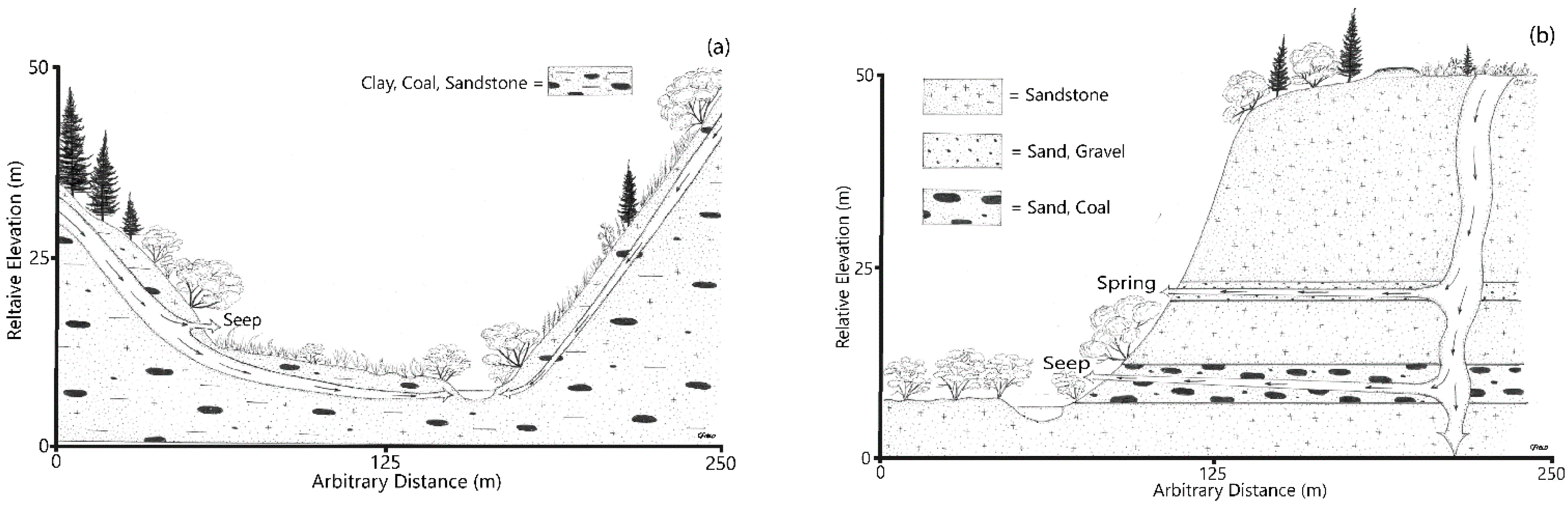
3.1. Types of Groundwater Discharge

Two types of groundwater discharge were identified in the study area, hillslope groundwater discharge and aquifer-outcrop groundwater discharge (Figure 3). Hillslope groundwater discharge occurs where rainfall and snowmelt infiltrate into the shallow subsurface, move laterally downslope through the shallow subsurface, and discharge as diffuse seeps and small springs at groundwater-induced slope failures and valley-bottom toeslopes. Aquifer-outcrop groundwater discharge occurs where rainfall and snowmelt infiltrate into the deep subsurface, move laterally through aquifers, and discharge as larger springs at aquifer outcrops in valleys carved by modern streams.

3.2. Manual Identification of Groundwater Discharge

3.2.1. Hillslope Groundwater Discharge

Hillslope groundwater discharge is likely to occur on large, concave, and steep hillslopes that accumulate, concentrate, and drive shallow groundwater downgradient toward concave midslope and/or toeslope positions. These factors are reflected in FWS, which is a function of the flow accumulation area and slope. FWS is partly a function of slope, so it tends to be highest in the steep terrain characteristic of the eastern section of the study area where high-elevation headwaters are common (Figure 2). Previous work in this study area has demonstrated that hillslopes with relatively moderate–high FWS are commonly associated with groundwater discharge to streams [12]. Flowlines are also a function of flow accumulation area. Therefore, a simple two-step workflow using FWS and flowlines was found to be sufficient for identifying locations where hillslope groundwater discharge was likely to occur, which could then be verified in the field (Figure 4).

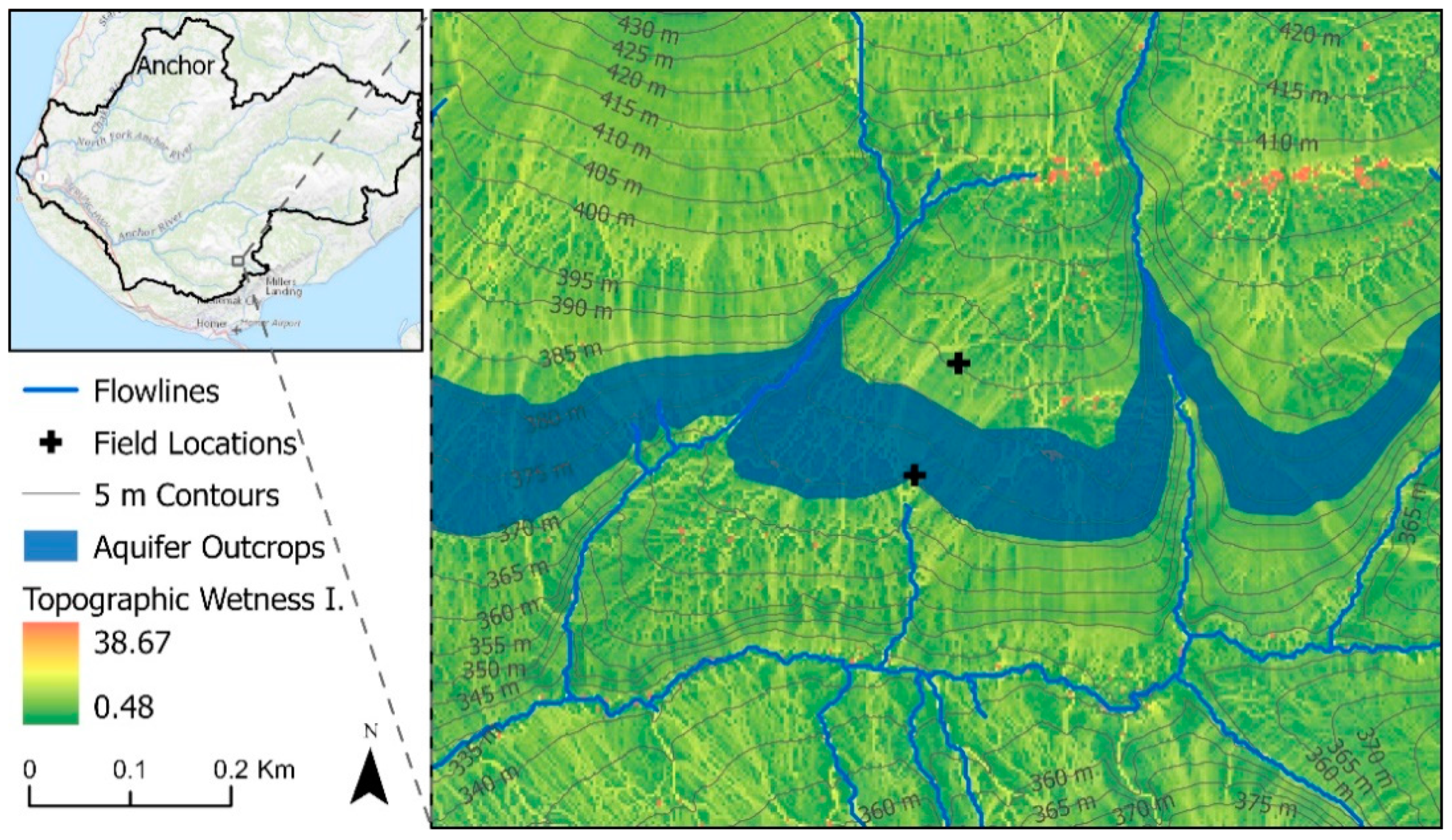
3.2.2. Aquifer-Outcrop Groundwater Discharge

Aquifer-outcrop groundwater discharge is likely to occur where aquifers outcrop and topography indicates the initiation of channelized flow. Aquifer outcrops are reflected in the aquifer outcrop layer, a created layer that covers only the western and southern, i.e., more-developed, settings where well log information was available (Figure 2). These aquifer outcrops commonly support large springs which form the headward extent of prominent channels, typically aligned roughly parallel to one another and abruptly initiating along the same contour interval. The spatially limited aquifer outcrop data product was then used to explore the topographic data that reflected the initiation of channelized flow, including the headward extent of incised topography, the initiation of flowlines, and the sudden concentration of the TWI. Therefore, a simple four-step workflow using the aquifer outcrops overlaid on contour lines, flowlines, and TWI was found to be sufficient for identifying locations where aquifer-outcrop groundwater discharge was likely to occur, which could then be verified in the field (Figure 5).

3.2.3. Field Verification

The procedures for identifying groundwater discharge were field verified by visiting 67 field locations, 54 where groundwater discharge was predicted to occur and 13 where groundwater discharge was predicted not to occur. Groundwater discharge was logged as occurring if a seep or spring was observed within 30 m of the predicted location. Results are tabulated in a confusion matrix (Table 1). The sensitivity (i.e., correctly predicted positives/total actual positives) is 50/51, or 98%, while the precision (i.e., correctly predicted positives/total predicted positives) is 50/54, or 93%. Accuracy, calculated as the percentage of correct predictions, is 62/67, or 93%. That is, overall, the manual procedures accurately predicted the presence or absence of groundwater discharge in 93% of cases. The kappa coefficient (κ), which takes into account the possibility of the agreement occurring by chance, is 0.78, which indicates substantial strength of agreement with the field data [77,78].

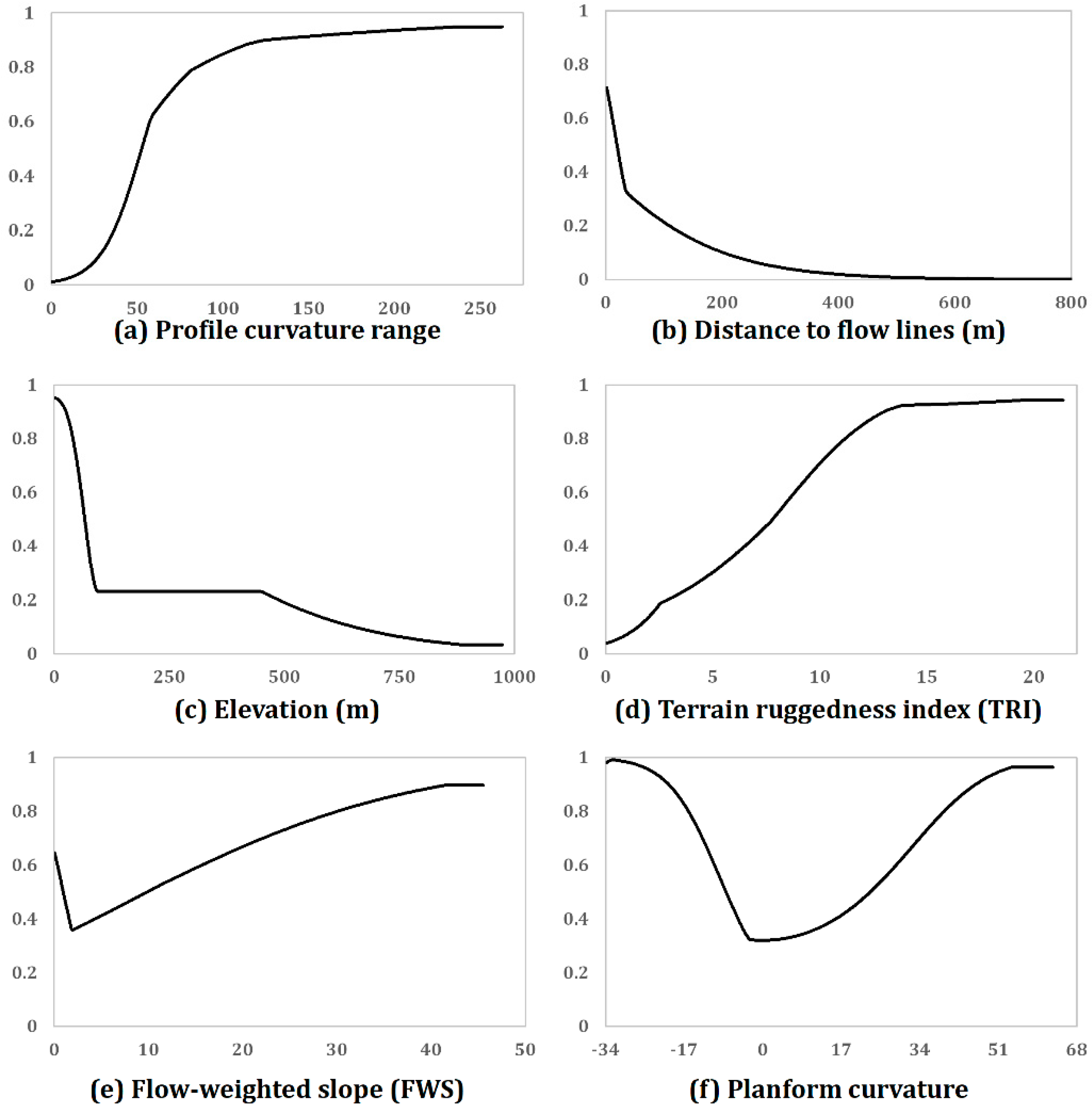
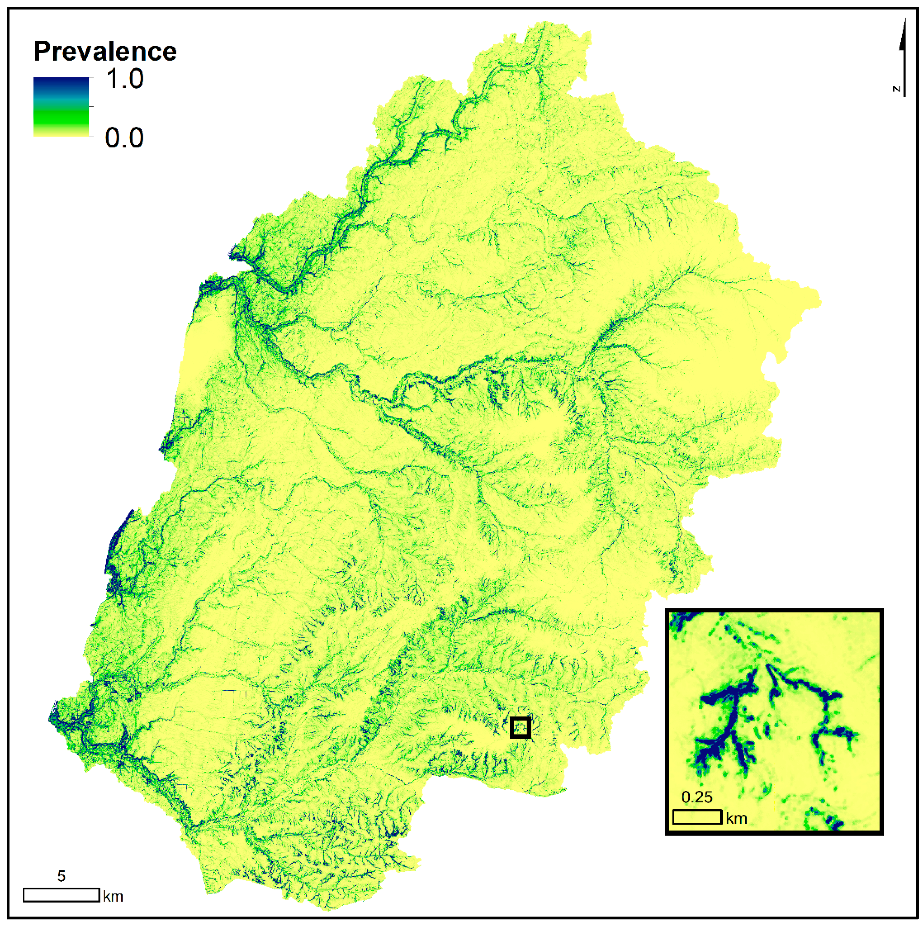
3.3. Modeled Identification of Groundwater Discharge

The final Maxent model included six topographic variables. Profile curvature range contributed the most information to the model with a permutation importance of 43.2%, followed by distance to flowlines, elevation, TRI, FWS, and planform curvature, with permutation importance of 20.8%, 18.5%, 15.2%, 1.8%, and 0.5%, respectively (Table 2). Predicted prevalence of seeps and springs was highest where profile curvature ranges were large, distances to flowlines were low, elevation was low, TRI was high (i.e., terrain was rugged), FWS was high, and planform curvature values were large (Figure 6). Collectively, the model predicts groundwater discharge where topography changes abruptly over small distances in close proximity to flowlines at lower elevations (Figure 7). The model predicts that seeps and springs are widespread over the study area, with high prevalence locations particularly at the headward extent of and alongside streams and along coastal bluffs. The AUC values for the model were 0.95 for training data and 0.91 for testing data, indicating outstanding performance [79].

4. Discussion

Though the primary controls on groundwater flow and discharge are climate, geology, and topography [37], we demonstrated that the locations where groundwater discharge occurs can be predicted based solely on topography if key diagnostic topographic signatures can be first identified using ancillary field observations and geologic data in a representative subset of the study area. Here, we modeled two types of groundwater discharge: hillslope groundwater discharge and aquifer-outcrop groundwater discharge (Figure 3). We constructed a robust geodatabase comprising field observations and geologic data from >800 well logs covering a representative subset of the study area and topographic data from an airborne LiDAR-derived DEM covering the entire study area (Figure 2). We then developed and refined procedures to manually identify the two types of groundwater discharge in the representative subset of the study area where the field observations, geologic data, and topographic data were available (Table 1; Figure 4 and Figure 5). While doing so, we made observations that indicated we might otherwise identify these two types of groundwater discharge using only the topographic data. We therefore developed and refined procedures to model the two types of groundwater discharge throughout the entire study area from the topographic data alone (Table 2; Figure 7). Devito et al. [43] previously argued that topography was the last control to consider in explaining hydrologic processes, after climate and geology. Rahmati et al. [30] concurred, suggesting that geologic data (e.g., lithology) was a relatively strong predictor of groundwater levels while topographic data (e.g., slope) was a relatively weak predictor of groundwater levels. Here, topography was in fact the only control we considered, but only after topography was contextualized with the field observations and geologic data in the representative subset of the study area.
The modeling benefited greatly from previous field observations by Callahan et al. [12], which in turn benefited greatly from other previous field observations by Walker et al. [66] and King et al. [80]. These studies showed that topography correlates with the structure and function of streams in the Kenai Peninsula Lowlands, including stream flow and stream water temperature [12], stream water chemistry [66], and stream biota [80]. These studies were conducted at 18 shared study sites in the Anchor River, Stariski Creek, Deep Creek, and Ninilchik Creek watersheds, four of the five watersheds included in this study. Callahan et al. [12] made the key insight that motivated our study. Their field observations indicated that a topographic feature, i.e., FWS, could be used to predict the location of hillslope groundwater discharge to streams. We further refined this understanding, noting that, for example, hillslopes with high FWS also had a prevalence of small headwater streams that originated at seeps and small springs. These are evident in the topographic data in a number of ways, including sudden changes in curvature (i.e., profile curvature range), flowlines, and TWI (Figure 2). This then allowed the accurate manual and modeled identification of hillslope groundwater discharge (Figure 4 and Figure 7).
The modeling also benefited greatly from the availability of >800 publicly available well logs (Figure 2). Surficial geology data are available for the entirety of the Kenai Peninsula Lowlands, at the 1:350,000 scale [59]. Such data can be useful in predicting potential groundwater recharge zones (e.g., [81]). However, such coarse data alone cannot be used to map thin confined aquifers and their outcrops, as was necessary for this study. The well logs allowed us to do so. Then subsequent field work further allowed us to refine our understanding of the spatial scale over which the well logs were predictive of aquifer outcrops (Figure 2). This allowed us to find numerous springs, which we then used to explore the topographic data that reflected the initiation of channelized flow, including the headward extent of incised topography, the initiation of flowlines, and the sudden concentration of the TWI. Once these relationships were identified, the topography could in many cases be used as a proxy for the geology, such as in cases where aquifer outcrops were instead indicated by the initiation of multiple, parallel channelized flows along the same contour intervals on the same and/or opposite hillslopes (e.g., Figure 5). This then allowed the accurate manual and modeled identification of aquifer-outcrop groundwater discharge (Table 2; Figure 5 and Figure 7).
The novelty of our modeling approach lies in the integration between field observations, remote-sensing data, and machine learning. Workflows for the manual identification of groundwater discharge were used to locate hillslope and aquifer-outcrop groundwater discharges in the field, with an overall accuracy of 93% (Table 1; Figure 4 and Figure 5). Though labor-intensive, this approach enabled the field identification of a large enough sample of seep and spring locations to develop an “outstanding” predictive model for the entire study area using topographic data alone, with an AUC of 0.95 and 0.91 for training and testing data, respectively (Table 2; Figure 7). Using only topographic data was ideal in our study area because well logs and therefore crucial geologic data (i.e., aquifer-outcrop locations) were only available over ~40% of the study area. Maxent modeling in particular was advantageous because it uses presence-only data and therefore can be used to make widespread predictions over a large study area with limited data over only a subset of the study area (e.g., [82]). Another advantage of the Maxent approach is its ability to quantify the relationships between feature prevalence and the environmental predictors [72,73]. Our model confirms field observations that groundwater discharge is most likely to occur where topography changes abruptly over small distances in close proximity to flowlines, supporting the findings of other studies (e.g., [2,46,47,63]).
Both field observations and modeling results indicate that seeps and springs are commonly located proximal to streams, both the headward extent of streams and along hillslopes adjacent to streams (e.g., Figure 7). Following the five major Pleistocene glaciations and two minor post-Pleistocene glacial advances, the Kenai Peninsula Lowlands comprised mixed ice-scoured landforms, drift sheets, and moraines separated by unconformities and weathering profiles, much covered with younger glacial outwash and valley train, glaciolacustrine, and other minor moraine deposits [58,59]. This heterogeneity was reflected at the surface, where local topographic relief was sufficient to direct surface-water flows into the earliest watersheds, and in the subsurface, where aquifers were commonly thin and discontinuous, often formed in thin glacial outwash and valley train deposits. Subsequent downcutting by the streams shaped and steepened valley hillslopes, thereby creating and enhancing hillslope groundwater discharge, and exposed aquifer outcrops, thereby creating and enhancing aquifer-outcrop groundwater discharge (Figure 3). This enhanced stream flow and therefore stream power, creating a positive feedback which further enhanced downcutting by the streams.
This groundwater discharge is essential for the proper functioning of streams on the Kenai Peninsula Lowlands. Groundwater discharge to these streams augments stream flow, providing approximately half of the summer stream flow and likely all of the winter stream flow [12]. Groundwater discharge to these streams also modulates stream temperatures, providing cold-water refugia in summer and warm-water refugia in winter [12]. Salmonids are cold-water species with life-history stages sensitive to high stream water temperatures, including sublethal temperatures which can affect everything from cellular function to behavior [83,84]. Therefore, cold-water refugia in summer are crucial, and increasingly so in light of climate-induced warming trends in Alaska’s salmon-bearing streams [85]. Juvenile salmonids must overwinter in these streams prior to outmigrating the following spring. Therefore, warm-water refugia in winter are also crucial, keeping some reaches unfrozen and available as overwintering habitats [86]. Lastly, much of this groundwater first passes through and interacts with nitrogen-fixing alder patches on adjacent hillslopes, delivering nitrogen-rich groundwater to riparian wetlands and these streams [14], where it enhances primary productivity in the riparian wetlands [14,87] and controls rates of in-stream nitrogen fixation and respiration [15,85]. The nutrient subsidies to these streams are then evident in the juvenile salmonids, who preferentially use abundant allochthonous sources, especially in the headwater settings [88]. Groundwater discharge is therefore thought to at least partly explain the predictable species composition along specific reaches in these streams, especially in headwater settings [66]. This new understanding of the importance of groundwater discharge to proper functioning of streams on the Kenai Peninsula Lowlands has led to groundwater being adopted as a central feature of the conceptual model underlying the management of the salmonid resources that underlie important sport and commercial fisheries [49].
Meanwhile, groundwater is the primary source of water for domestic, commercial, and industrial uses on the Kenai Peninsula Lowlands [52]. Most wells are domestic and are drilled by, maintained, and operated at the sole discretion and expense of the individual landowner. Drilling costs are calculated per unit depth, so there is little incentive to drill beyond the shallowest aquifer that can provide sufficient quantities of water. Well logs indicate that these aquifers are thin and discontinuous and commonly yield ~0.01–0.1 m3/min (see also [60]). These then are the same aquifers that often outcrop on nearby hillslopes, commonly at the headward extent of streams and along hillslopes adjacent to streams (e.g., Figure 3 and Figure 7). These aquifers are therefore the nexus of a potential conflict over limited groundwater resources between natural and human users. These results have heightened awareness, with recent and ongoing work focused on using this new understanding to explore sources and locations of acute groundwater vulnerability and connecting this new understanding to decision-making by building capacity to support both peer and institutional discussions [49].

Author Contributions

This paper was the result of a broad, collaborative effort by all authors. Conceptualization, M.C.R.; Methodology, M.E.G., K.C.R., E.J.G.-O., J.D. and M.C.R.; Validation, M.E.G., K.C.R., E.J.G.-O., W.J.K., J.D. and M.C.R.; Formal Analysis, M.E.G., E.J.G.-O. and J.D.; Investigation, M.E.G., K.C.R., E.J.G.-O., W.J.K., J.D., S.M.L. and M.C.R.; Data Curation, M.E.G., K.C.R., E.J.G.-O. and S.M.L.; Writing—Original Draft Preparation, M.E.G. and M.C.R.; Writing—Review & Editing, K.C.R., E.J.G.-O., W.J.K., J.D. and S.M.L.; Visualization, S.M.L. and J.D.; Supervision, K.C.R. and M.C.R.; Project Administration, K.C.R. and M.C.R.; Funding Acquisition, M.C.R. All authors have read and agreed to the published version of the manuscript.

Funding

This research was funded primarily by the National Estuarine Research Reserve System Science Collaborative under Grant No. 54584 (https://nerrssciencecollaborative.org/project/Walker17; accessed on 23 December 2021). Additional faculty support was funded by the National Science Foundation under Grant No. 1702029 (https://www.nsf.gov/awardsearch/showAward?AWD_ID=1702029; accessed on 23 December 2021). Additional student scholarships were funded by the National Science Foundation under Grant No. 1930451 (https://nsf.gov/awardsearch/showAward?AWD_ID=1930451; accessed on 23 December 2021).

Institutional Review Board Statement

Not applicable.

Informed Consent Statement

Not applicable.

Data Availability Statement

Publicly available datasets were analyzed in this study. This data can be found here: doi:10.6084/m9.figshare.16586903.

Acknowledgments

This project benefitted immeasurably from in-kind support provided by the Kachemak Bay National Estuarine Research Reserve, which provided lodging, local knowledge, introductions to stakeholders, the coordination of formal stakeholder engagements, and more. Coowe Walker and Syverine Bentz were particularly instrumental. Conrad Field illustrated Figure 3 from field sketches and notes prepared by M Rains. Annalyssa Hernandez assisted in some field work. A special thank you to all of the many stakeholders who provided their time, local knowledge, and access to private properties.

Conflicts of Interest

The authors declare no conflict of interest.

References

  1. Rains, M.C.; Fogg, G.E.; Harter, T.; Dahlgren, R.A.; Williamson, R.J. The role of perched aquifers in hydrological connectivity and biogeochemical processes in vernal pool landscapes, Central Valley, California. Hydrol. Process. 2006, 20, 1157–1175. [Google Scholar] [CrossRef]
  2. Neff, B.P.; Rosenberry, D.O.; Leibowitz, S.G.; Mushet, D.M.; Golden, H.E.; Rains, M.; Brooks, J.R.; Lane, C.R. A Hydrologic Landscapes Perspective on Groundwater Connectivity of Depressional Wetlands. Water 2019, 12, 50. [Google Scholar] [CrossRef] [PubMed] [Green Version]
  3. Kornelsen, K.; Coulibaly, P. Synthesis review on groundwater discharge to surface water in the Great Lakes Basin. J. Great Lakes Res. 2014, 40, 247–256. [Google Scholar] [CrossRef]
  4. Solana, M.X.; Londoño, O.M.Q.; Romanelli, A.; Donna, F.; Martínez, D.E.; Weinzettel, P. Connectivity of temperate shallow lakes to groundwater in the Pampean Plain, Argentina: A remote sensing and multi-tracer approach. Groundw. Sustain. Dev. 2021, 13, 100556. [Google Scholar] [CrossRef]
  5. Winter, T.C.; Harvey, J.W.; Franke, O.L.; Alley, W.M. Ground Water and Surface Water: A Single Resource; Circular 1139; US Geological Survey: Reston, VA, USA, 1998. [Google Scholar] [CrossRef]
  6. Winter, T.C. Relation of streams, lakes, and wetlands to groundwater flow systems. Hydrogeol. J. 1999, 7, 28–45. [Google Scholar] [CrossRef]
  7. Moore, W.S.; Blanton, J.O.; Joye, S. Estimates of flushing times, submarine groundwater discharge, and nutrient fluxes to Okatee Estuary, South Carolina. J. Geophys. Res. Space Phys. 2006, 111, 111. [Google Scholar] [CrossRef]
  8. Moore, W.S. The Effect of Submarine Groundwater Discharge on the Ocean. Annu. Rev. Mar. Sci. 2010, 2, 59–88. [Google Scholar] [CrossRef] [Green Version]
  9. Misra, D.; Daanen, R.P.; Thompson, A.M. Base Flow/Groundwater Flow. In Encyclopedia of Snow, Ice and Glaciers; Encyclopedia of Earth Sciences Series; Singh, V.P., Singh, P., Haritashya, U.K., Eds.; Springer: Dordrecht, The Netherlands, 2011. [Google Scholar]
  10. Guérin, A.; Devauchelle, O.; Robert, V.; Kitou, T.; Dessert, C.; Quiquerez, A.; Allemand, P.; Lajeunesse, E. Stream-Discharge Surges Generated by Groundwater Flow. Geophys. Res. Lett. 2019, 46, 7447–7455. [Google Scholar] [CrossRef] [Green Version]
  11. Caissie, D. The thermal regime of rivers: A review. Freshw. Biol. 2006, 51, 1389–1406. [Google Scholar] [CrossRef]
  12. Callahan, M.K.; Rains, M.; Bellino, J.C.; Walker, C.M.; Baird, S.J.; Whigham, D.F.; King, R.S. Controls on Temperature in Salmonid-Bearing Headwater Streams in Two Common Hydrogeologic Settings, Kenai Peninsula, Alaska. JAWRA J. Am. Water Resour. Assoc. 2014, 51, 84–98. [Google Scholar] [CrossRef] [Green Version]
  13. Luke, S.H.; Luckai, N.J.; Burke, J.M.; Prepas, E.E. Riparian areas in the Canadian boreal forest and linkages with water quality in streams. Environ. Rev. 2007, 15, 79–97. [Google Scholar] [CrossRef]
  14. Callahan, M.K.; Whigham, D.F.; Rains, M.; Rains, K.C.; King, R.S.; Walker, C.M.; Maurer, J.R.; Baird, S.J. Nitrogen Subsidies from Hillslope Alder Stands to Streamside Wetlands and Headwater Streams, Kenai Peninsula, Alaska. JAWRA J. Am. Water Resour. Assoc. 2017, 53, 478–492. [Google Scholar] [CrossRef]
  15. Hiatt, D.L.; Robbins, C.J.; Back, J.A.; Kostka, P.K.; Doyle, R.D.; Walker, C.M.; Rains, M.C.; Whigham, D.F.; King, R.S. Catchment-scale alder cover controls nitrogen fixation in boreal headwater streams. Freshw. Sci. 2017, 36, 523–532. [Google Scholar] [CrossRef] [Green Version]
  16. Power, G.; Brown, R.S.; Imhof, J.G. Groundwater and Fish—Insights from Northern North America. Hydrol. Process. 1999, 13, 401–422. [Google Scholar] [CrossRef]
  17. Dieter, C.A.; Maupin, M.A.; Caldwell, R.R.; Harris, M.A.; Ivahnenko, T.I.; Lovelace, J.K.; Barber, N.L.; Linsey, K.S. Estimated Use of Water in the United States in 2015; Circular 1441; US Geological Survey: Reston, VA, USA, 2018. [Google Scholar] [CrossRef]
  18. Falkenmark, M.; Rockström, J. Balancing Water for Humans and Nature: The New Approach in Ecohydrology; Earthscan: London, UK; Sterling, VA, USA, 2004; ISBN 978-1-85383-927-6. [Google Scholar]
  19. Khalil, M.A.; Bobst, A.; Mosolf, J. Utilizing 2D Electrical Resistivity Tomography and Very Low Frequency Electromagnetics to Investigate the Hydrogeology of Natural Cold Springs Near Virginia City, Southwest Montana. Pure Appl. Geophys. PAGEOPH 2018, 175, 3525–3538. [Google Scholar] [CrossRef]
  20. Gleason, C.L.; Frisbee, M.D.; Rademacher, L.K.; Sada, D.W.; Meyers, Z.P.; Knott, J.R.; Hedlund, B.P. Hydrogeology of desert springs in the Panamint Range, California, USA: Geologic controls on the geochemical kinetics, flowpaths, and mean residence times of springs. Hydrol. Process. 2020, 34, 2923–2948. [Google Scholar] [CrossRef]
  21. Mocior, E.; Rzonca, B.; Siwek, J.; Plenzler, J.; Płaczkowska, E.; Dabek, N.; Jaskowiec, B.; Potoniec, P.; Roman, S.; Zdziebko, D. Determinants of the distribution of springs in the upper part of a flysch ridge in the Bieszczady Mountains in southeastern Poland. Episodes 2015, 38, 21–30. [Google Scholar] [CrossRef] [Green Version]
  22. Howard, J.; Merrifield, M. Mapping Groundwater Dependent Ecosystems in California. PLoS ONE 2010, 5, e11249. [Google Scholar] [CrossRef] [Green Version]
  23. Pourtaghi, Z.S.; Pourghasemi, H.R. GIS-based groundwater spring potential assessment and mapping in the Birjand Township, southern Khorasan Province, Iran. Hydrogeol. J. 2014, 22, 643–662. [Google Scholar] [CrossRef]
  24. Lange, H.; Sippel, S. Machine Learning Applications in Hydrology. In Forest-Water Interactions; Levia, D.F., Carlyle-Moses, D.E., Iida, S., Michalzik, B., Nanko, K., Tischer, A., Eds.; Ecological Studies; Springer International Publishing: Cham, Switzerland, 2020; Volume 240, pp. 233–257. ISBN 978-3-030-26085-9. [Google Scholar]
  25. Nearing, G.S.; Kratzert, F.; Sampson, A.K.; Pelissier, C.S.; Klotz, D.; Frame, J.M.; Prieto, C.; Gupta, H.V. What Role Does Hydrological Science Play in the Age of Machine Learning? Water Resour. Res. 2021, 57, e2020WR028091. [Google Scholar] [CrossRef]
  26. Shen, C.; Chen, X.; Laloy, E. Editorial: Broadening the Use of Machine Learning in Hydrology. Front. Water 2021, 3, 681023. [Google Scholar] [CrossRef]
  27. Sahoo, S.; Russo, T.A.; Elliott, J.; Foster, I. Machine learning algorithms for modeling groundwater level changes in agricultural regions of the U.S. Water Resour. Res. 2017, 53, 3878–3895. [Google Scholar] [CrossRef]
  28. Rahman, A.S.; Hosono, T.; Quilty, J.M.; Das, J.; Basak, A. Multiscale groundwater level forecasting: Coupling new machine learning approaches with wavelet transforms. Adv. Water Resour. 2020, 141, 103595. [Google Scholar] [CrossRef]
  29. Afan, H.A.; Osman, A.I.A.; Essam, Y.; Ahmed, A.N.; Huang, Y.F.; Kisi, O.; Sherif, M.; Sefelnasr, A.; Chau, K.-W.; El-Shafie, A. Modeling the fluctuations of groundwater level by employing ensemble deep learning techniques. Eng. Appl. Comput. Fluid Mech. 2021, 15, 1420–1439. [Google Scholar] [CrossRef]
  30. Rahmati, O.; Pourghasemi, H.R.; Melesse, A.M. Application of GIS-based data driven random forest and maximum entropy models for groundwater potential mapping: A case study at Mehran Region, Iran. Catena 2016, 137, 360–372. [Google Scholar] [CrossRef]
  31. El Bilali, A.; Taleb, A.; Brouziyne, Y. Groundwater quality forecasting using machine learning algorithms for irrigation purposes. Agric. Water Manag. 2021, 245, 106625. [Google Scholar] [CrossRef]
  32. Shiri, N.; Shiri, J.; Yaseen, Z.M.; Kim, S.; Chung, I.-M.; Nourani, V.; Zounemat-Kermani, M. Development of artificial intelligence models for well groundwater quality simulation: Different modeling scenarios. PLoS ONE 2021, 16, e0251510. [Google Scholar] [CrossRef] [PubMed]
  33. Tan, Z.; Yang, Q.; Zheng, Y. Machine Learning Models of Groundwater Arsenic Spatial Distribution in Bangladesh: Influence of Holocene Sediment Depositional History. Environ. Sci. Technol. 2020, 54, 9454–9463. [Google Scholar] [CrossRef] [PubMed]
  34. Tran, D.A.; Tsujimura, M.; Ha, N.T.; Nguyen, V.T.; Van Binh, D.; Dang, T.D.; Doan, Q.-V.; Bui, D.T.; Ngoc, T.A.; Phu, L.V.; et al. Evaluating the predictive power of different machine learning algorithms for groundwater salinity prediction of multi-layer coastal aquifers in the Mekong Delta, Vietnam. Ecol. Indic. 2021, 127, 107790. [Google Scholar] [CrossRef]
  35. Hussein, E.A.; Thron, C.; Ghaziasgar, M.; Bagula, A.; Vaccari, M. Groundwater Prediction Using Machine-Learning Tools. Algorithms 2020, 13, 300. [Google Scholar] [CrossRef]
  36. Jaafarzadeh, M.S.; Tahmasebipour, N.; Haghizadeh, A.; Pourghasemi, H.R.; Rouhani, H. Groundwater recharge potential zonation using an ensemble of machine learning and bivariate statistical models. Sci. Rep. 2021, 11, 1–18. [Google Scholar] [CrossRef]
  37. Winter, T.C. The concept of hydrologic landscapes. JAWRA J. Am. Water Resour. Assoc. 2001, 37, 335–349. [Google Scholar] [CrossRef]
  38. Wolock, D.M.; Winter, T.C.; McMahon, G. Delineation and Evaluation of Hydrologic-Landscape Regions in the United States Using Geographic Information System Tools and Multivariate Statistical Analyses. Environ. Manag. 2004, 34, S71–S88. [Google Scholar] [CrossRef] [PubMed]
  39. Wigington, P.J.; Leibowitz, S.G.; Comeleo, R.L.; Ebersole, J. Oregon Hydrologic Landscapes: A Classification Framework1. JAWRA J. Am. Water Resour. Assoc. 2012, 49, 163–182. [Google Scholar] [CrossRef]
  40. Brydsten, L. Modelling Groundwater Discharge Areas Using Only Digital Elevation Models as Input Data; Swedish Nuclear Fuel and Waste Management: Stockholm, Sweden, 2006; p. 18. [Google Scholar]
  41. Tweed, S.O.; Leblanc, M.; Webb, J.; Lubczynski, M.W. Remote sensing and GIS for mapping groundwater recharge and discharge areas in salinity prone catchments, southeastern Australia. Hydrogeol. J. 2006, 15, 75–96. [Google Scholar] [CrossRef]
  42. Haitjema, H.M.; Mitchell-Bruker, S. Are Water Tables a Subdued Replica of the Topography? Ground Water 2005, 43, 781–786. [Google Scholar] [CrossRef] [PubMed]
  43. Devito, K.; Creed, I.; Gan, T.; Mendoza, C.; Petrone, R.; Silins, U.; Smerdon, B. A framework for broad-scale classification of hydrologic response units on the Boreal Plain: Is topography the last thing to consider? Hydrol. Process. 2005, 19, 1705–1714. [Google Scholar] [CrossRef]
  44. Toth, J. Groundwater discharge: A common generator of diverse geologic and morphologic phenomena. Int. Assoc. Sci. Hydrol. Bull. 1971, 16, 7–24. [Google Scholar] [CrossRef]
  45. Huang, X.; Niemann, J.D. Modelling the potential impacts of groundwater hydrology on long-term drainage basin evolution. Earth Surf. Process. Landforms 2006, 31, 1802–1823. [Google Scholar] [CrossRef]
  46. Iverson, R.M.; Reid, M.E. Gravity-driven groundwater flow and slope failure potential: 1. Elastic Effective-Stress Model. Water Resour. Res. 1992, 28, 925–938. [Google Scholar] [CrossRef]
  47. Reid, M.E.; Iverson, R.M. Gravity-driven groundwater flow and slope failure potential: 2. Effects of slope morphology, material properties, and hydraulic heterogeneity. Water Resour. Res. 1992, 28, 939–950. [Google Scholar] [CrossRef]
  48. UACED (University of Alaska Center for Economic Development). Kenai Peninsula 2021–2026 Comprehensive Economic Development Strategy; Kenai Peninsula Economic Development District: Kenai, AK, USA, 2021; p. 97. [Google Scholar]
  49. Walker, C.M.; Whigham, D.F.; Bentz, I.S.; Argueta, J.M.; King, R.S.; Rains, M.C.; Simenstad, C.A.; Guo, C.; Baird, S.J.; Field, C.J. Linking landscape attributes to salmon and decision-making in the southern Kenai Lowlands, Alaska, USA. Ecol. Soc. 2021, 26, 1. [Google Scholar] [CrossRef]
  50. ADLWD (Alaska Department of Labor and Workforce Development). Alaska Population Projections 2019–2045; Alaska Department of Labor and Workforce Development: Juneau, AK, USA, 2020.
  51. HSWCD (Homer Soil and Water Conservation District). Growing Local Food: A Survey of Commercial Producers on the Southern Kenai Peninsula; Homer Soil and Water Conservation District: Homer, AK, USA, 2018. [Google Scholar]
  52. Glass, R. Ground-Water Conditions and Quality in the Western Part of Kenai Peninsula, Southcentral Alaska; Open-File Rep. 96-446; US Geological Survey: Reston, VA, USA, 1996. [Google Scholar] [CrossRef]
  53. Baughman, C.A.; Loehman, R.A.; Magness, D.R.; Saperstein, L.B.; Sherriff, R.L. Four Decades of Land-Cover Change on the Kenai Peninsula, Alaska: Detecting Disturbance-Influenced Vegetation Shifts Using Landsat Legacy Data. Land 2020, 9, 382. [Google Scholar] [CrossRef]
  54. Klein, E.; Berg, E.E.; Dial, R. Wetland drying and succession across the Kenai Peninsula Lowlands, south-central Alaska. Can. J. For. Res. 2005, 35, 1931–1941. [Google Scholar] [CrossRef]
  55. Berg, E.E.; Hillman, K.M.; Dial, R.; DeRuwe, A. Recent woody invasion of wetlands on the Kenai Peninsula Lowlands, south-central Alaska: A major regime shift after 18 000 years of wet Sphagnum–sedge peat recruitment. Can. J. For. Res. 2009, 39, 2033–2046. [Google Scholar] [CrossRef]
  56. Magness, D.R.; Morton, J.M. Using climate envelope models to identify potential ecological trajectories on the Kenai Peninsula, Alaska. PLoS ONE 2018, 13, e0208883. [Google Scholar] [CrossRef] [PubMed] [Green Version]
  57. USGS (U.S. Geological Survey). The National Map U.S. Geological Survey’s (USGS) National Geospatial Program. Available online: https://www.usgs.gov/core-science-systems/national-geospatial-program/national-map (accessed on 30 August 2021).
  58. Karlstrom, T.N. Quaternary Geology of the Kenai Lowland and Glacial History of the Cook Inlet Region, Alaska; Professional Paper 443; US Geological Survey: Reston, VA, USA, 1964. [Google Scholar] [CrossRef]
  59. Wilson, F.H.; Hults, C.P. Geology of the Prince William Sound and Kenai Peninsula Region, Alaska; Scientific Investigations Map 3110; US Geological Survey: Anchorage, AK, USA, 2012. [Google Scholar] [CrossRef] [Green Version]
  60. Nelson, G.; Johnson, P. Ground-Water Reconnaissance of Part of the Lower Kenai Peninsula, Alaska; Open-File Rep. 81-905; US Geological Survey: Reston, VA, USA, 1981. [Google Scholar] [CrossRef]
  61. Spencer, E.W. Geologic Maps: A Practical Guide to Preparation and Interpretation; Waveland Press: Long Grove, IL, USA, 2017; ISBN 1-4786-3488-X. [Google Scholar]
  62. Heine, R.A.; Lant, C.L.; Sengupta, R.R. Development and Comparison of Approaches for Automated Mapping of Stream Channel Networks. Ann. Assoc. Am. Geogr. 2004, 94, 477–490. [Google Scholar] [CrossRef]
  63. Jaeger, K.L.; Montgomery, D.R.; Bolton, S.M. Channel and Perennial Flow Initiation in Headwater Streams: Management Implications of Variability in Source-Area Size. Environ. Manag. 2007, 40, 775–786. [Google Scholar] [CrossRef] [Green Version]
  64. Detty, J.M.; McGuire, K.J. Topographic controls on shallow groundwater dynamics: Implications of hydrologic connectivity between hillslopes and riparian zones in a till mantled catchment. Hydrol. Process. 2010, 24, 2222–2236. [Google Scholar] [CrossRef]
  65. Riley, S.J.; DeGloria, S.D.; Elliot, R. A Terrain Ruggedness Index That Quantifies Topographic Heterogeneity. Intermt. J. Sci. 1999, 5, 23–27. [Google Scholar]
  66. Korzeniowska, K.; Pfeifer, N.; Landtwing, S. Mapping gullies, dunes, lava fields, and landslides via surface roughness. Geomorphology 2018, 301, 53–67. [Google Scholar] [CrossRef]
  67. Walker, C.M.; King, R.S.; Whigham, D.F.; Baird, S.J. Landscape and Wetland Influences on Headwater Stream Chemistry in the Kenai Lowlands, Alaska. Wetlands 2012, 32, 301–310. [Google Scholar] [CrossRef]
  68. Beven, K.J.; Kirkby, M.J. A physically based, variable contributing area model of basin hydrology/Un modèle à base physique de zone d’appel variable de l’hydrologie du bassin versant. Hydrol. Sci. Bull. 1979, 24, 43–69. [Google Scholar] [CrossRef] [Green Version]
  69. Sørensen, R.; Zinko, U.; Seibert, J. On the calculation of the topographic wetness index: Evaluation of different methods based on field observations. Hydrol. Earth Syst. Sci. 2006, 10, 101–112. [Google Scholar] [CrossRef] [Green Version]
  70. Tarboton, D. A new method for the determination of flow directions and upslope areas in grid digital elevation models. Water Resour. Res. 1997, 33, 309–319. [Google Scholar] [CrossRef] [Green Version]
  71. Horvath, E.K.; Christensen, J.R.; Mehaffey, M.H.; Neale, A.C. Building a potential wetland restoration indicator for the contiguous United States. Ecol. Indic. 2017, 83, 463–473. [Google Scholar] [CrossRef]
  72. Rains, M.; Mount, J.F. Origin of shallow ground water in an alluvial aquifer as determined by isotopic and chemical procedures. Ground Water 2002, 40, 552–563. [Google Scholar] [CrossRef] [PubMed]
  73. Phillips, S.J.; Dudík, M. Modeling of species distributions with Maxent: New extensions and a comprehensive evaluation. Ecography 2008, 31, 161–175. [Google Scholar] [CrossRef]
  74. Elith, J.; Phillips, S.J.; Hastie, T.; Dudík, M.; Chee, Y.E.; Yates, C.J. A statistical explanation of MaxEnt for ecologists. Divers. Distrib. 2011, 17, 43–57. [Google Scholar] [CrossRef]
  75. Merow, C.; Smith, M.J.; Silander, J.A. A practical guide to MaxEnt for modeling species’ distributions: What it does, and why inputs and settings matter. Ecography 2013, 36, 1058–1069. [Google Scholar] [CrossRef]
  76. Feng, X.; Park, D.S.; Liang, Y.; Pandey, R.; Papeş, M. Collinearity in ecological niche modeling: Confusions and challenges. Ecol. Evol. 2019, 9, 10365–10376. [Google Scholar] [CrossRef] [Green Version]
  77. Cohen, J. A Coefficient of Agreement for Nominal Scales. Educ. Psychol. Meas. 1960, 20, 37–46. [Google Scholar] [CrossRef]
  78. Landis, J.R.; Koch, G.G. An Application of Hierarchical Kappa-type Statistics in the Assessment of Majority Agreement among Multiple Observers. Biometrics 1977, 33, 363. [Google Scholar] [CrossRef]
  79. Mandrekar, J.N. Receiver Operating Characteristic Curve in Diagnostic Test Assessment. J. Thorac. Oncol. 2010, 5, 1315–1316. [Google Scholar] [CrossRef] [Green Version]
  80. King, R.S.; Walker, C.M.; Whigham, D.F.; Baird, S.J.; Back, J.A. Catchment topography and wetland geomorphology drive macroinvertebrate community structure and juvenile salmonid distributions in south-central Alaska headwater streams. Freshw. Sci. 2012, 31, 341–364. [Google Scholar] [CrossRef] [Green Version]
  81. Souissi, D.; Msaddek, M.H.; Zouhri, L.; Chenini, I.; El May, M.; Dlala, M. Mapping groundwater recharge potential zones in arid region using GIS and Landsat approaches, southeast Tunisia. Hydrol. Sci. J. 2018, 63, 251–268. [Google Scholar] [CrossRef]
  82. Rhoden, C.M.; Peterman, W.E.; Taylor, C.A. Maxent-directed field surveys identify new populations of narrowly endemic habitat specialists. PeerJ 2017, 5, e3632. [Google Scholar] [CrossRef] [PubMed] [Green Version]
  83. Taylor, S.G. Climate warming causes phenological shift in Pink Salmon, Oncorhynchus gorbuscha, behavior at Auke Creek, Alaska. Glob. Chang. Biol. 2008, 14, 229–235. [Google Scholar] [CrossRef]
  84. Bowen, L.; von Biela, V.R.; McCormick, S.D.; Regish, A.M.; Waters, S.C.; Durbin-Johnson, B.; Britton, M.; Settles, M.L.; Donnelly, D.S.; Laske, S.M.; et al. Transcriptomic response to elevated water temperatures in adult migrating Yukon River Chinook salmon (Oncorhynchus tshawytscha). Conserv. Physiol. 2020, 8, coaa084. [Google Scholar] [CrossRef]
  85. Shaftel, R.S.; King, R.S.; Back, J.A. Breakdown rates, nutrient concentrations, and macroinvertebrate colonization of bluejoint grass litter in headwater streams of the Kenai Peninsula, Alaska. J. N. Am. Benthol. Soc. 2011, 30, 386–398. [Google Scholar] [CrossRef]
  86. Gutsch, M.K. Dentification and Characterization of Juvenile Coho Salmon Overwintering Habitats and Early Spring Outmigration in the Anchor River Watershed, Alaska; University of Alaska, Fairbanks: Fairbanks, AK, USA, 2011. [Google Scholar]
  87. Whigham, D.; Walker, C.; Maurer, J.; King, R.; Hauser, W.; Baird, S.; Keuskamp, J.; Neale, P. Watershed influences on the structure and function of riparian wetlands associated with headwater streams—Kenai Peninsula, Alaska. Sci. Total Environ. 2017, 599, 124–134. [Google Scholar] [CrossRef] [PubMed]
  88. Dekar, M.P.; King, R.S.; Back, J.A.; Whigham, D.; Walker, C.M. Allochthonous inputs from grass-dominated wetlands support juvenile salmonids in headwater streams: Evidence from stable isotopes of carbon, hydrogen, and nitrogen. Freshw. Sci. 2012, 31, 121–132. [Google Scholar] [CrossRef]
Figure 1. General location of the five watersheds that comprise the study area on the Kenai Peninsula Lowlands. Base map source [57].
Remotesensing 14 00063 g001
Figure 2. Primary geologic and topographic layers include: (a) well log points and modeled aquifer outcrops; (b) DEM, represented by a shaded relief to emphasize terrain, with the 67 field points used for training and testing; (c) flowlines; (d) TRI; (e) FWS; and (f) TWI. Here, only the Anchor River Watershed, the southernmost of the five watersheds, is shown in full.
Remotesensing 14 00063 g002
Figure 3. Types of groundwater discharge include (a) hillslope groundwater discharge and (b) aquifer-outcrop groundwater discharge. Illustrations drawn by Conrad Field from field sketches and notes prepared by Mark Rains.
Remotesensing 14 00063 g003
Figure 4. Example of implementing the two-step workflow to locate hillslope groundwater discharge. FWS is first used to identify hillslopes with relatively high FWS. Flowlines are then used to identify specific locations where channels may initiate. Diffuse seeps are commonly found in these settings, including at the field location in this example.
Remotesensing 14 00063 g004
Figure 5. Example of implementing the four-step workflow to locate aquifer-outcrop groundwater discharge. Aquifer outcrops are first used to indicate regions where large volumes of groundwater discharge likely occur. Then each of the three topographic layers, i.e., contour lines, the initiation of flowlines, and sudden increases in TWI, are used to identify locations where channelized flows initiate. Springs are commonly found in these settings. In this case, the lowermost field point was preselected and found in the field to be 13 m from a spring. The uppermost field point was then visited, and the static water level was found to be ~2 m below the ground surface in a hand-dug well.
Remotesensing 14 00063 g005
Figure 6. Predicted probability of prevalence (y-axis) for six topographic variables used in the final Maxent model to predict seeps and springs: (a) profile curvature range, (b) distance to flowlines, (c) elevation, (d) TRI, (e) FWS, and (f) planform curvature. The curves represent the dependence of predicted prevalence on both the individual topographic variables and the correlations between them.
Remotesensing 14 00063 g006
Figure 7. Predicted prevalence of seeps and springs in the entire study area. Seeps and springs are most likely to occur where spring prevalence values are highest. The inset highlights the small box in the southeast of the study area, which is an example area where the probability of the occurrence of seeps and springs is particularly high.
Remotesensing 14 00063 g007
Table 1. Confusion matrix of ground-truth points collected to verify the accuracy of the geodatabase predictions.
Predicted NoPredicted YesTotal
Actual No12416
Actual Yes15051
Total135467
Table 2. Permutation importance for variables used to predict seeps and springs using the Maxent model.
VariablePermutation Importance (%)
Profile curvature range43.2
Distance to flowlines20.8
Elevation18.5
Terrain ruggedness index15.2
Flow-weighted slope1.8
Planform curvature0.5
Publisher’s Note: MDPI stays neutral with regard to jurisdictional claims in published maps and institutional affiliations.

