1. Introduction
Remote sensing has been used across the globe to assess in-field crop conditions. Within-field variability has been documented in many crop parameters, such as biomass and leaf [
1], plant height in cotton (
Gossypium hirsutum L.; [
2]), yield in wheat (
Triticum aestivum L.; [
3]) and maize (
Zea mays L.; [
4]). Moreover, monitoring the in-season maturity of species, such as soybean (
Glycine max L.), has also been viable through the use of remote sensing and vegetation indices (VIs) derived from high-resolution imagery [
5]. Preliminary studies with proximal optical sensing in peanut (
Arachis hypogaea L.) plots with different planting dates indicated that maturity may be estimated with VIs [
6]. These observations, however, were likely the result of biomass differences.
Maturity prediction in peanut has been challenging as there are no obvious aboveground indicators of maturity. Peanut pods, the fruit of the crop, are produced underground. After fertilization of the flower, a stalk, commonly referred to as the peg, elongates with the ovary and grows down into the soil. The tip of the peg then develops into a mature peanut pod [
7]. Because peanut is an indeterminate crop, it produces flowers for extended periods during the growing season. As a result, peanut pods of varying maturity are present on the plant as the harvest period approaches. Therefore, determining optimum maturity is difficult. Harvesting a field at peak maturity results in the highest seed quality, grade, and yields. Immature pods generally have seeds with lower oil content, thus decreasing quality [
8]. On the other hand, harvesting plants with over-mature pods results in yield losses of up to 40% because the pods detach from the pegs during the inversion process, and are lost to the soil [
9].
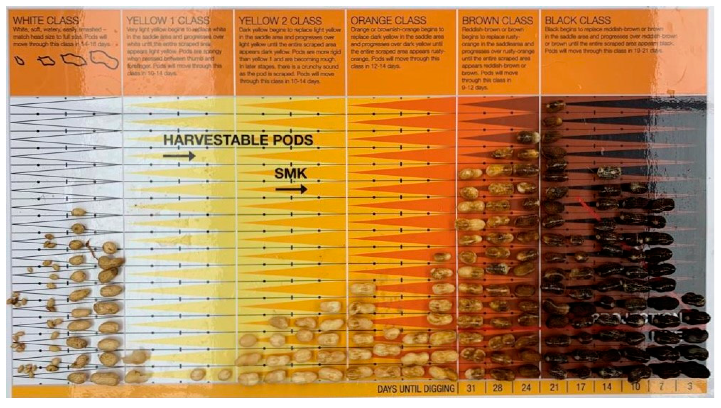
Williams et al. [
10] observed that as peanut pods mature, the mesocarp (second layer of the pod’s hull) changes color from white to yellow, orange, brown, and finally black when they are fully mature. The authors then developed the hull-scrape method for determining peanut maturity. This method has been widely used by peanut producers in the U.S. and other countries. However, sorting the pods by color and placing them on the board is subjective and highly dependent on the sorter’s color perception.
An additional strategy used to predict maturity in peanut is the adjusted cumulative growing-degree days (aGDD). This strategy is based on calculation of the heat accumulated by the crop [
11]. The model uses daily maximum and minimum temperatures, a base temperature of 13.3 °C for peanut, evapotranspiration, and water (precipitation and irrigation, if available). U.S. runner-type peanut usually achieves optimum maturity at approximately 2500 aGDDs [
11]. The aGDD technique still requires confirmation of maturity using the hull-scrape method.
To standardize the assessment of maturity percentage in a sample, Rowland et al. [
11] developed the peanut maturity index (PMI) for runner-type peanut. PMI is the percentage of mature pods (brown + black classes) of the overall sample. Generally, the hull-scrape method is labor intensive, subjectively based on a person’s ability to place pods in the correct color category, and subjected to field microvariability that may affect the maturity of individual plants.
Digital RGB image analysis has also been tested for peanut maturity classification. Ghate et al. [
12] developed a system to classify peanut pods into three categories—immature, medium maturity, and fully mature—according to the visual texture of the hulls. Moreover, a software model of digital color classification was trained to identify peanut maturity by scanning pods in different orientations (saddle region up or randomly placed) in a commercial scanner and further calculating the maturity percentage [
13]. Although the maturity analysis through RGB images reduces the subjectivity of the human eye, the method is still laborious and time consuming, since the pods must be collected in the field and the mesocarp exposed prior to the image being taken, and the pods must be rotated during imaging. Clearly, alternatives that estimate pod maturity across the entire field rather than individual plants would assist producers to make better harvest decisions.
The growing use of remote sensing techniques in peanut production has contributed new insights on maturity prediction with decreased subjectivity, while capturing field-scale conditions without destructively sampling plants. Rowland et al. [
14] found that the reflectance in the near infrared (NIR) band was more strongly correlated with peanut maturity when compared to other bands. Changes in peanut reflectance in the red edge (RE) band as pods approach maturity indicate that these wavelengths are also sensitive to pod maturity [
15]. Vegetation indices derived from the reflectance bands have been shown to be a promising tool for monitoring maturity. Several studies have been performed to evaluate VIs as indicators of peanut maturity, but they were unable to identify an index that consistently predicted peanut maturity [
14,
15,
16,
17]. Yu et al. [
5] used a tractor-mounted optical reflectance sensor to evaluate the response of VIs to peanut maturity in a plot-scale study. The authors found that Non-Linear Index (NLI) was the most accurate predictor of maturity for many peanut varieties. However, additional research is needed to determine whether VIs can be successfully used to predict pod maturity in peanut plants.
In recent years, Machine Learning (ML) tools have been increasingly used, especially in relation to remote sensing techniques to solve non-linear problems [
18]. Among the numerous ML models, artificial neural networks (ANN) have been used to identify complex patterns in agricultural systems [
19]. Although the use of a non-linear model to identify the ideal maturity point of peanut pods through remote sensing has been previously reported [
20], research using ML tools to explain the variability in estimating maturity has not been documented for peanut. The objectives of this study were to (I) compare the efficiency of using linear and multiple linear regression with models using ANN and (II) verify the accuracy of ANN models to predict peanut maturity in irrigated and rainfed areas.
2. Materials and Methods
2.1. Study Sites
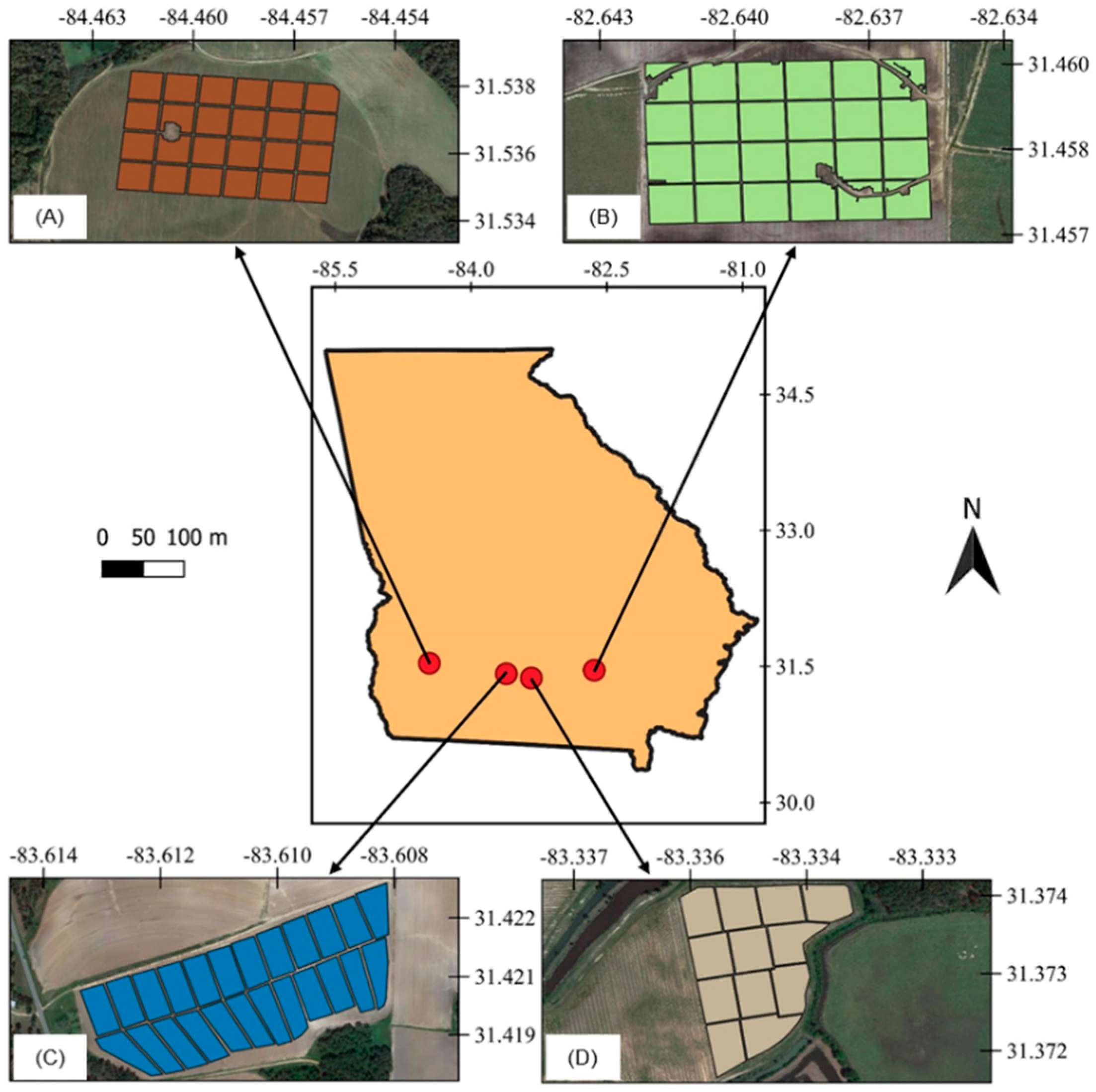
Four commercial peanut fields located in southern Georgia, U.S., one irrigated and one rainfed from each of the 2018 and 2019 growing seasons, were used in this study (
Figure 1). The irrigated and rainfed fields from 2018 were planted on June 6 and June 11, respectively. In 2019, the irrigated field was planted on April 29 and the rainfed field was planted on April 28. The peanut runner-type cultivar Georgia-06G was used in all fields, which has a growing cycle of approximately 140 days and is planted in over 90% of peanut fields in Georgia [
21].
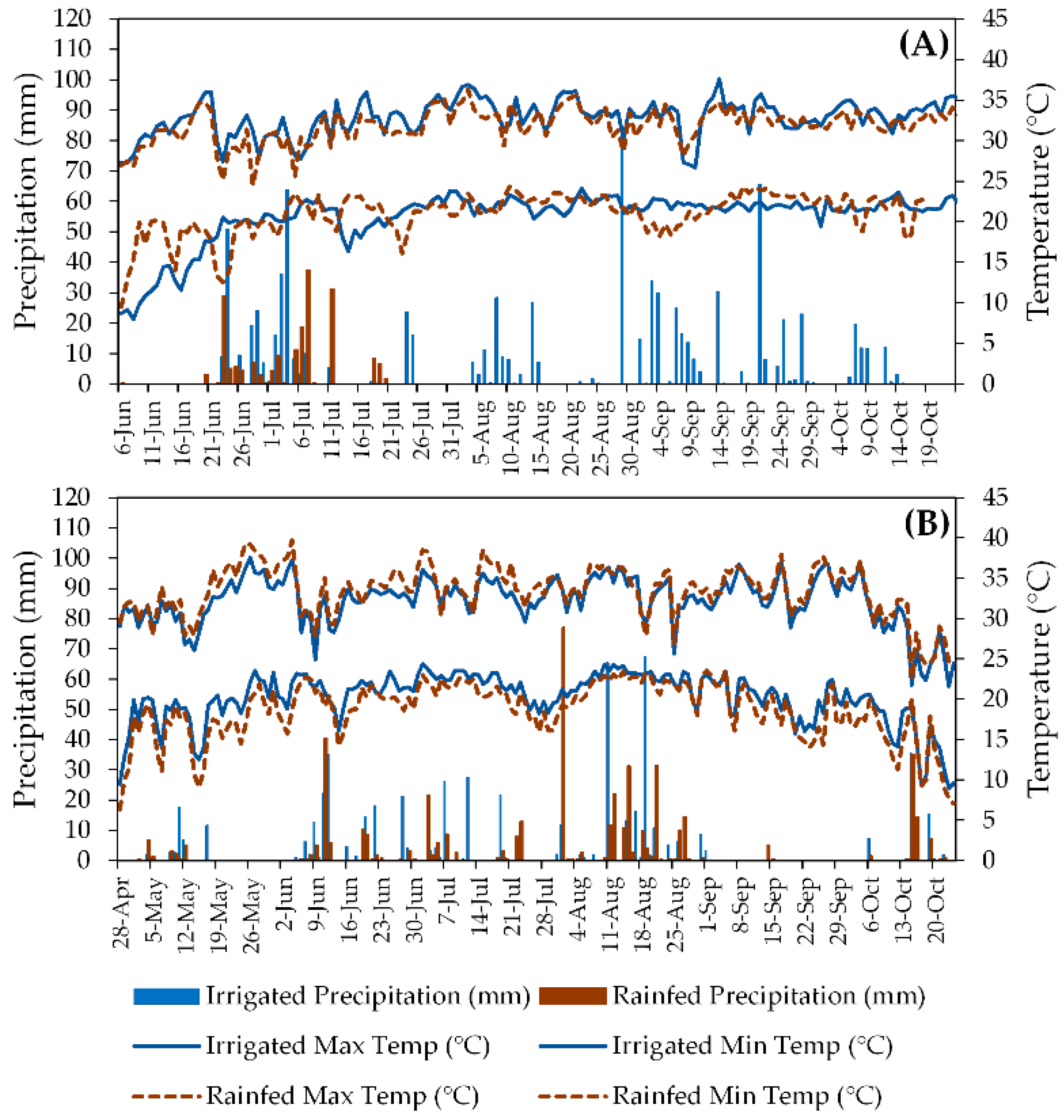
Southern Georgia has a subtropical climate, with hot summers (classified as Cfa according to [
22]) and average annual precipitation of 1346 mm. Coupled with the region’s sandy soils, these environmental conditions are favorable for peanut production, especially when irrigation is available. Daily maximum and minimum temperatures and daily precipitation for the experimental sites in both seasons are presented in
Figure 2.
2.2. Ground Data Collection
In the 2018 and 2019 irrigated fields and the 2018 rainfed field, a 24 ha area within the field was selected for the study. Because the 2019 rainfed field was smaller, a 12 ha area was selected for the study. The study areas were divided into 1 ha plots (
Figure 2). Starting 90 days after planting (DAP), 10 plants were collected weekly in a 10 m radius from the center of each plot. The plants were transferred to the laboratory and the pods were manually detached from the plants until approximately 200 pods were reached for each sample. Occasionally, the required number of pods was achieved using less than 10 plants, so not all plants from each plot or sampling time were always used. After detaching from the plants, the pods were pressure-washed in order to expose the mesocarp color following the protocol given in Williams et al. [
10]. The pods were then placed on the Peanut Profile Board according to mesocarp color (
Figure 3) and the number of pods in each maturity class was recorded [
10]. Optimum maturity is achieved when the leading edge of the sample maturity profile reaches the sloped line on the board. PMI was calculated for each sample according to [
14] by dividing the number of mature pods (brown + black) by the sum of the total pods in the sample. PMI varies from 0 to 1 and optimal maturity occurs when a sample has a PMI of 0.7.
For each sampling time, adjusted cumulative growing degree days (aGDDs) was calculated using the daily evapotranspiration, maximum and minimum temperatures, and precipitation [
11]. The PeanutFARM (peanutfarm.org, 5 November 2021) crop management tool was used to automatically retrieve the meteorological parameters from a weather station closest to each field and calculate the aGDDs.
2.3. UAV Data Collection and Image Processing
During each sampling time, a Parrot Sequoia camera (Parrot Drone SAS, Paris, France) mounted on a 3DR Solo (3D Robotics, Berkeley, CA, USA) quadcopter was used to obtain multispectral images in 4 different bands, Green (530–570 nm), Red (640–680 nm), NIR (770–810 nm) and RE (730–740 nm). All UAV flights were performed within 2 h of solar noon with clear and cloudless weather conditions at an altitude of 90 m with 70% front and side overlap resulting in a resolution of approximately 95 mm per pixel. UAV image processing was performed using Pix4Dmapper software (Pix4D SA, Lausanne, Switzerland) version 4.4.12. Single images were stitched to create reflectance map mosaics of all four bands. During the stitching process, geographic correction was performed using four ground control points, with known coordinates distributed around the perimeter of the field. Calibration panel images taken after each flight were used to perform radiometric calibration of the final reflectance maps.
After the mosaics were created, soil background reflectance was removed from each band using unsupervised classification with ArcGIS software (ESRI, Redlands, CA, USA). A model was then developed using the same software to extract an average reflectance value for each of the 24 individual plots per date in both fields in 2018 and the irrigated field in 2019, and 12 individual plots per date in the rainfed area in 2019. In all fields, a 1 ha area with 10 m negative buffer at the edge of the plot was used for each plot’s average reflectance. Average reflectance values were used to develop VIs for each plot for each flight day.
2.4. Vegetation Indices
Eleven VIs that have been used in other studies to predict crop maturity were selected and evaluated using this study’s data (
Table 1).
2.5. Statistical Analysis
Different approaches were tested to predict peanut pod maturity based on canopy reflectance and aGDD, and they are described in the following sections.
2.5.1. Linear and Multiple Linear Regression
In summary, linear regression models are used to explain the spatial distribution using a dependent variable and independent variable (predictor). In this study, eleven VIs were calculated, and they were used individually as predictors in a linear model (LR) to explain PMI variability. A second step was performed to improve the LR models using multiple linear regression (MLR). In this case, aGGD was identified as having better performance to predict PMI; thus, it was combined with each single VI to create an MLR. In both models, we used 80% of the dataset for training and 20% for testing.
2.5.2. Artificial Neural Networks
For the non-linear model, artificial neural networks (ANNs) were used to test different input combinations (80% of the dataset for training and 20% for testing the models). The ANN methods used were Multilayer Perceptron (MLP) and Radial Basis Function (RBF). These two methods are widely used for complex data classification and prediction in precision agriculture. ANNs are systems that consist of artificial neurons, which perform similar functions to human neurons [
31]. Without assumptions on the data distribution, these algorithms can learn relationships among input and estimated variables [
32]. Furthermore, they are capable of solving complex problems that cannot be explained through linear models. The commonly adopted trial and error approach is time consuming and impractical to carry out manually related to hyperparameter optimization and feature selection. Therefore, Intelligent Problem Solver (IPS), a tool built into Statistica 7 software, was used. It combines heuristic and sophisticated optimization strategies (minimal-bracketing and simulated annealing algorithm, [
33]).
2.6. ANN Structure
The input layer for the ANNs consisted of VIs and spectral bands, whereas the output was the PMI. The number of neurons was variable, from one to 30 for the MLP networks and one to 45 for the RBF networks. The network inputs (VIs and aGDD) also varied as well as the number of hidden layers, from one to three for MLP and only one for RBF. All VIs described in
Table 1 as well as the individual bands and the aGDD were tested individually and combined. For each input combination, one thousand models were trained using the error backward propagation supervised learning algorithm for the MLP models [
34]. The backpropagation neural network is trained with inputs adjusted to output variables in two phases [
32]. The RBF is trained by the k-means algorithm [
35].
With boundaries defined (neural network types, number of neuron and hidden layer, inputs and output), a thousand models with different combinations of the parameter’s boundaries were trained using the IPS tool; using the balance error against diversity algorithm, ten models using the MLP network and ten models using the RBF network were retained and then the best model was selected based on accuracy and precision metrics calculated using a test dataset (20% of the data not used during the training process). All these approaches were performed for each scenario (irrigated, rainfed and pooled data from all fields).
2.6.1. MLP
MLP networks were interconnected by synaptic weights, which are responsible for storing the value of a connection between two nodes. Values used in the input layers were normalized according to Equation (1):
in which
xi is the input vector value (e.g., vegetation index) and
xmin and
xmax are the minimum and maximum observed values, respectively.
The output value of each neuron in layer
k is expressed by
zk =
g(
ak), in which
g is the activation function of
ak and
ak is the synaptic function, which is a linear combination of the normalized input values and the synaptic weights (Equation (2)).
in which
wkj are the synaptic weights connecting the
yj input values with each
k neuron.
The transfer or activation function in the neurons of each hidden layer was the hyperbolic tangent function, with ‘
e’ being the Napierian number (Equation (3)).
2.6.2. RBF
RBF networks have only one hidden layer and each neuron contains a radial basis activation function. In each neuron, the Gaussian or normal function was used as a radial basis function [
35], and the distance (deviation) values of this function increase or decrease in relation to the center point [
36]. The Gaussian function is presented in Equation (4):
in which
ν = ||x − µ|| is the Euclidean distance between the input vector and the center µ of the Gaussian function, and
σ is the width. The Euclidean distance from the input vector to the center; µ is the input to the Gaussian function, which provides the activation value of the radial unit.
The output of each neuron in the output layer is defined by Equation (5):
in which
is the synaptic weight between the neuron
in the hidden layer and the neuron
j of the output layer,
is the input data, and
is the Gaussian function of each neuron in the hidden layer.
As in the MLP neural network, the input values were normalized by Equation (2), in which the values in the output layer provided the estimated PMI.
2.7. Model Performance Evaluation
To evaluate the model performance for PMI prediction, the coefficients of determination (R
2) and root mean square error (RMSE) were calculated using Equations (6) and (7):
in which
n is the number of datapoints,
yest is the value of the variable estimated by the network, and
yobs is the value of the observed variable.
in which
SSR is the sum of squares of the regression and
TSS is the total sum of squares.
Models with higher R2 and lower RMSE (<0.07) predict PMI more accurately.
3. Results
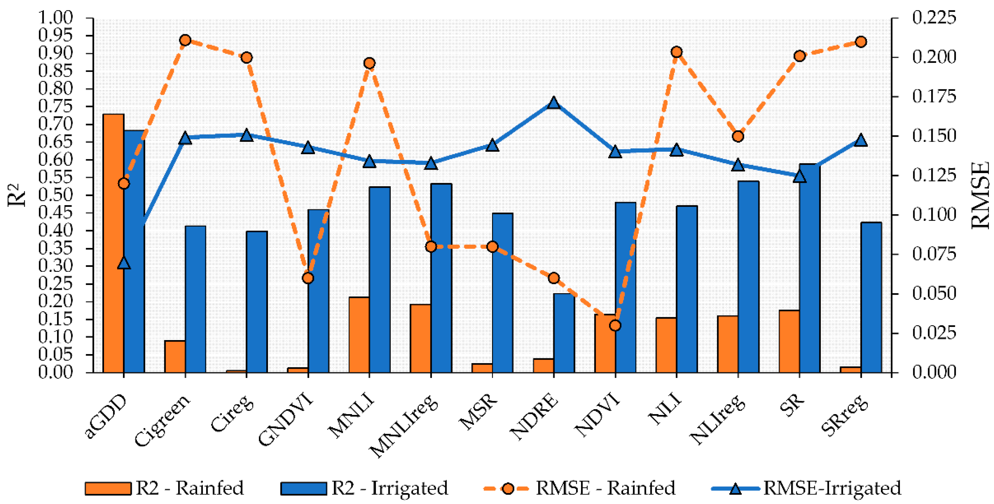
The performance of the VIs to predict peanut maturity varied across the growing conditions evaluated in this study. More accurate models to predict maturity using the linear model approach with VI as a predictor were obtained for the irrigated plots (
Figure 4). Of the evaluated VIs, SR had the highest R
2 and lowest RMSE (0.59 and 0.125, respectively) followed by NLIreg, MNLIreg, and MNLI, which had R
2 values higher than 0.50 and RMSE of approximately 0.133 (
Figure 4). These four VIs also had the highest model performance for predicting peanut maturity in the rainfed plots; however, the R
2 values were low (<0.20) and the RMSE, high. In addition, the linear models using MNLIreg, GNDVI, SRreg, and CIreg were not significant (
p > 0.05).
For both irrigated and rainfed areas, the most accurate linear fit model was observed when aGDD was used to estimate PMI (
Figure 4). This resulted in an R
2 of 0.73 for rainfed and 0.68 for irrigated fields. This indicates that using aGDD to predict peanut maturity is a sound approach because aGDD is associated with variables directly related to the phenological development of peanut plants.
The combination of VIs and aGDD in multiple linear models increased performance for both rainfed and irrigated plots but mostly under rainfed conditions (
Figure 5). However, despite significant F test values (
p < 0.05), the models using MSR-aGDD, MNLIreg-aGDD, SR-aGDD, NDRE-aGDD, and NLI-aGDD had non-significant values for the VI parameter within the multiple linear model, thus indicating that the maturity variability is better explained by the aGDD parameter (
p < 0.05) than by the use of the VIs mentioned above. Moreover, although the use of multiple linear models improved the precision and accuracy in estimating PMI, the model including NDVI as one of the predictors increased the error (RMSE) by 85%, from 0.030 in the linear model to 0.202 in the multiple linear model for the rainfed conditions during the test step.
The multiple linear models were further tested on a dataset different than the one used to generate the models and all of them overestimated the PMI patterns, regardless of the growing conditions (data not shown). Overestimating or underestimating values using linear models may be a consequence of the model learning process, in which the estimated values are only reliable if the predictors are within the same range of values as the data used to train the model. Therefore, the use of non-linear models can improve PMI prediction, especially when using VIs as predictors, which have high temporal and spatial variability, mainly when comparing irrigated versus rainfed areas.
Among over one thousand models tested using ANN, two were selected for irrigated and rainfed areas—RBF and MLP (
Table 2). In contrast with linear models, the PMI prediction through ANN can be performed in either irrigated and rainfed conditions with similar accuracy. However, the inputs and topology for each growing condition were different. A feature importance analysis is also shown in
Supplementary Table S1 for each ANN model. The input aGDD had the greatest importance in the model, except for MLP for the irrigated area, in which SRreg had the highest contribution (
Table S1).
The performance of the ANN models to predict PMI in irrigated fields during the training process was similar for the two models tested (RBF and MLP) in irrigated areas. Both models overestimated maturity at the beginning of the pod maturity process, yet errors were less than 10%. On the other hand, when maturity was greater than 60%, the RBF and MLP models had a lower number of errors in the training and test steps.
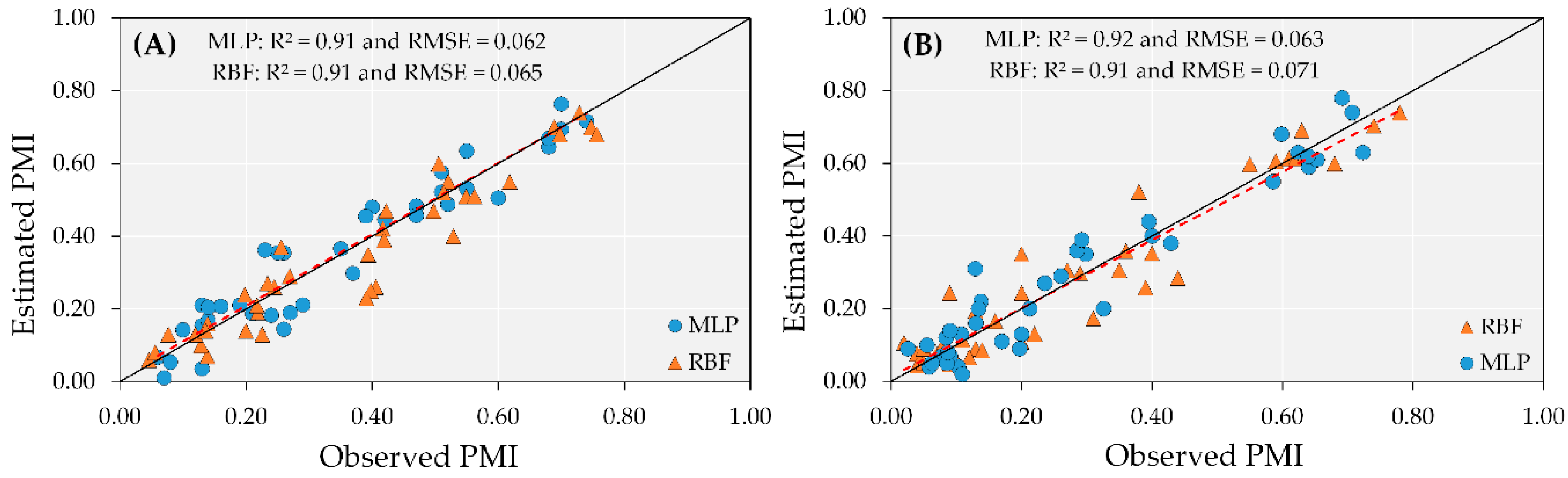
These results indicate that when plants reach high pod maturity (approaching the harvest period), the ANN models can be used to predict PMI with an accuracy of R
2 = 0.91 in irrigated areas, regardless of using RBF or MLP (
Figure 6A). Overall, the MLP model had a low RMSE (0.062) and a successful linear fit for the estimated by observed values (1:1 line) in the data test step, whereas the RBF model had RMSE of 0.065 (
Figure 6B).
Unlike linear models, which did not perform well during test, the use of ANNs shows great potential for predicting PMI in rainfed areas, even with variations in reflectance values among dates, which occurred more often in 2019, when plants experienced more drought periods (
Figure 3 and
Figure 6). The interaction between water and plant is complex and directly affects the maturity process, increasing the variability in the canopy reflectance and the percentage of mature pods within the same plant. Even in these variable conditions, the test accuracy for the MLP and RBF had R
2 = 0.92 and 0.91, respectively (
Figure 6).
In addition, both models had a lower number of errors for the prediction at the beginning of the sampling period, when the plants had accumulated between 1600 to 1900 aGDDs. As the PMI variability increased (middle of the growing season), RBF tended to underestimate the values, whereas MLP maintained values on the 1:1 line (
Figure 6). Error values lower than 8% suggested that ANN models were able to estimate peanut maturity in rainfed areas with high precision and accuracy.
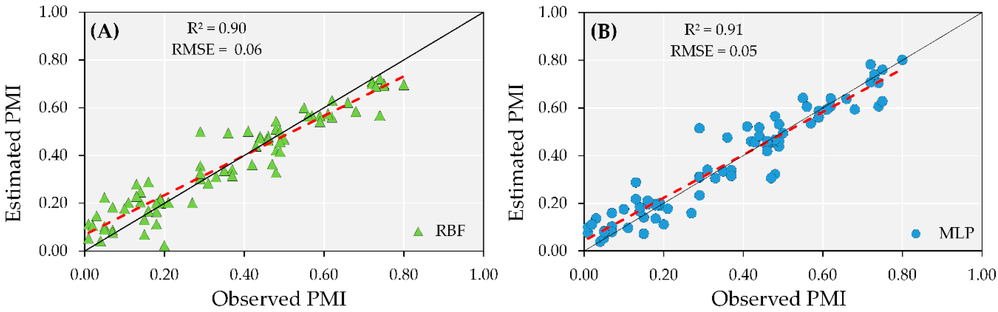
The combination of data from irrigated and rainfed areas was tested to train a robust and overall PMI prediction model capable of estimating maturity, regardless of growing conditions. Maximum errors found during the training step were 0.038 for RBF and 0.033 for MLP when observed PMI values were between 30 and 40%. However, the error for both ANN models decreased when the observed PMI values were greater than 60%, with errors below 0.005.
The test results of the overall model (irrigated and rainfed combined) indicated R
2 greater than 0.90 and similar RMSE for both ANN models tested, with errors of 0.07 (
Figure 7). Despite the accuracy of the overall models using ANN, during the test step, both models overestimated the PMI at early maturity stages and underestimated it when the observed maturity was greater than 70%. These results in the test step suggest that the accuracy in PMI prediction is high; however, the irrigation conditions for a given field should be taken into consideration.
Analyzing the performance of the algorithms LR, MLR, and ANN considering their best input combinations for greater accuracy, for both irrigated and rainfed conditions, the ANN models were the most accurate (
Figure 4,
Figure 5,
Figure 6 and
Figure 7). Each LR considered a single VI in the model (
Figure 4), whereas the MLR models used a combination of a given VI and aGG (
Figure 5). For the ANN, aGG was combined with multiple VIs in each model (
Table 2). The use of multiple inputs in the ANN models allows for solving complex problems, which has been widely used in agriculture. These results emphasize the greater learning ability and agriculture applications of ANN compared with less complex prediction models (e.g., LR or MLR), mainly for the peanut crop.
4. Discussion
The use of VIs to predict peanut maturity is a promising alternative to reduce the subjectivity of the current method based on pod mesocarp color [
10], especially when the VIs are associated with aGDD. This is especially important since peanut pods are developed belowground and the lants have indeterminate growth habits, which increases the complexity of determining the optimal harvest time. Monitoring the peanut crop with multispectral images acquired with a UAV indicated that all VI values decreased in magnitude as plants approached the optimal inverting (digging) time. These results corroborate work reported by dos Santos et al. [
20], in which peanut plants were monitored with high-resolution satellite images (3 m) and an optimal inverting time was predicted using the Gompertz model. The successful outcome of that study is tempered by the difficulty in obtaining cloud-free satellite images during the growing season in humid peanut growing regions such as southern Georgia where partial cloud cover is a daily occurrence during the growing season. This generally limits the number of useful images available, even for satellite platforms with high temporal resolution, and can be especially critical as harvest approaches. Although acquiring images with UAVs is also subject to problems associated with clouds, UAVs provide much higher scheduling flexibility and the window of time needed to fly over a field is relatively small, thus providing more opportunity to collect cloud-free images.
Different degrees of index saturation or soil background can affect VIs [
37]. NDVI and NLI had similar performance using linear models (
Figure 4), since both indices are calculated using the same bands with similar equations. NDVI is particularly sensitive to saturation under full canopy cover conditions. However, in the NLI equation, the NIR reflectance value is squared to attenuate saturation effects. Although NLI is an improved VI derived from NDVI, both VIs were saturated and remained relatively constant until 2200 aGDD in the irrigated fields because of canopy closure prior to the first flights. Between 2326 and 2400 aGDD, both VIs decreased by 50% (data not shown) as the plants approached maturity. This is because of the changing trends in red and NIR reflectance during this period associated with physiological changes. Reduction in VI values in the peanut crop is directly associated with leaf area index (LAI), with red and NIR being the most sensitive bands to biomass variation [
38].
On the other hand, VIs had lower values and greater variability among plots for the rainfed area, which may have affected the accuracy of the linear models. This is likely because the VIs responded to the effect of the spatial variability of soils on plant growth that was exaggerated under rainfed conditions compared to irrigated conditions. Under irrigated conditions, crop water stress can be better managed and promote more uniform growth across the field despite underlying soil variability [
39,
40,
41]. This difference in VIs between the irrigated and rainfed fields is related to reflectance in the NIR, in which reflectance in this band is more evident than in the visible spectrum in plants under stress.
Despite the low accuracy of the linear and multiple linear models obtained in this study, especially in the test process, the relationship between PMI and VI was previously demonstrated by means of linear fit, in which Rowland et al. [
14] observed greater sensitivity to leaf changes for NDVI compared to GNDVI, mainly when the short-wave infrared reflectance (SWIR—1640 nm) was combined with red (660 nm) using a spectroradiometer.
The multiple linear models using VIs and aGDD were moderately satisfactory with R
2 greater than 0.55 and RMSE less than 0.135, except when combining NDVI and aGDD. The ANN models outperformed the linear and multiple linear regressions in predicting PMI. The separation of effects is valid in the multiple linear regression approach when the hypotheses are true [
42]. This has the advantage of identifying the contribution of a given parameter to the model. In our study, aGDD was the parameter with greatest contribution to predict PMI through a multiple linear regression model. Although, aGDD alone was not sufficient to predict optimal pod maturity with high precision. The use of mathematical models through artificial intelligence with multiple inputs, such as the RBF and MLP networks tested in this study, showed that it is possible to reduce subjectivity with high accuracy and precision when using plant reflectance and meteorological data, reducing human intervention at the classification process. In addition, the ANN models can identify the influence that each variable has on the PMI response, and this advantage is due to parallel processing in the interaction of inputs [
42].
The ANN models observed in our study showed the highest accuracy among all models developed to explain the relationship between VIs and PMI through remote sensing reported in the literature [
14,
15,
20]. Regardless of the ANN architecture used in our study, both considered aGDD as the input, which strengthened the power in PMI prediction by these models, which is a unique contribution to the science. In addition, it was demonstrated that the use of a specific model is recommended for each growing condition, mainly related to differences in weather conditions across years and land areas (e.g., irrigation availability). In rainfed fields, although the ANN models have shown high accuracy both for the training and test processes, the precision and accuracy of the prediction models must be associated with weather variables, mainly precipitation, since under low precipitation conditions, drought stress can be a confounding factor estimating PMI through remote sensing.


 ,
, 


