
A Novel Real-Time Echo Separation Processing Architecture for Space–Time Waveform-Encoding SAR Based on Elevation Digital Beamforming

 ,
,  , , , , and
Abstract
:1. Introduction
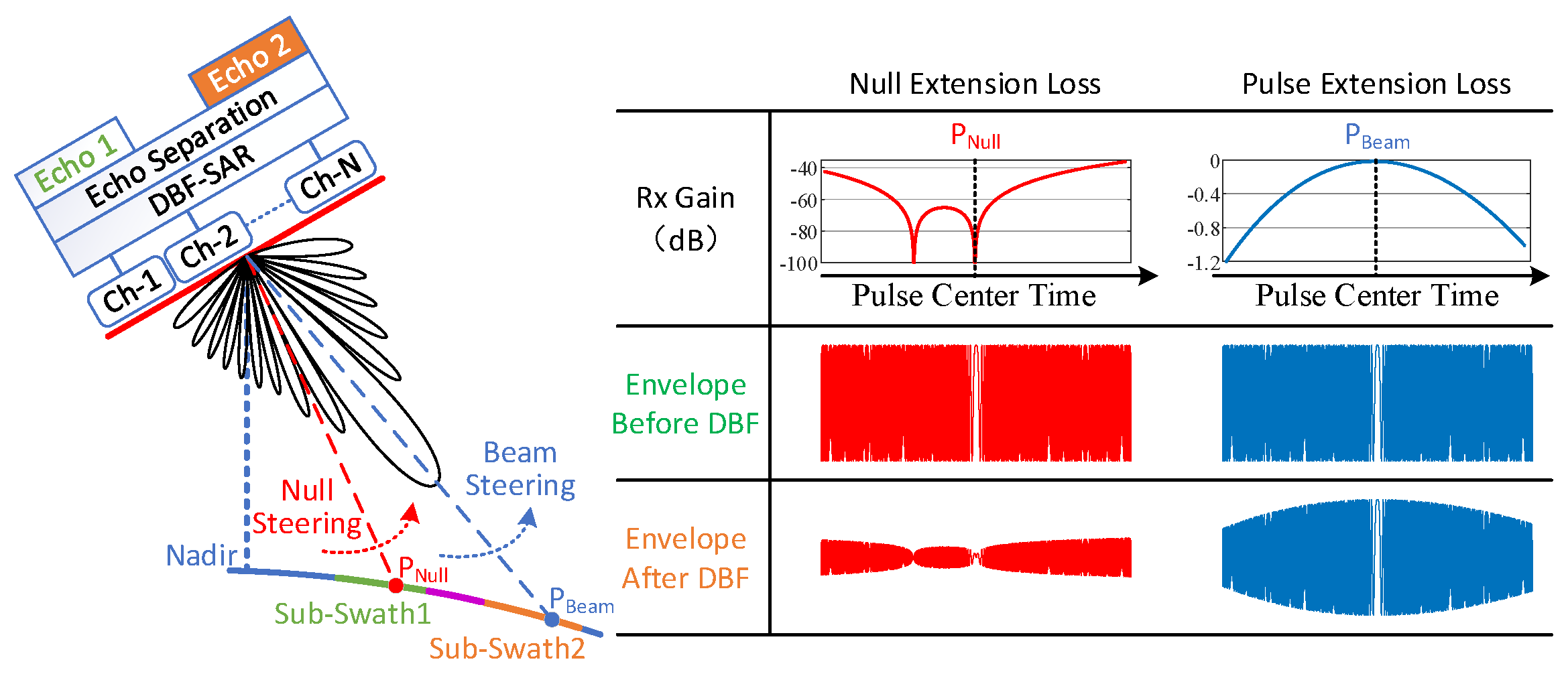
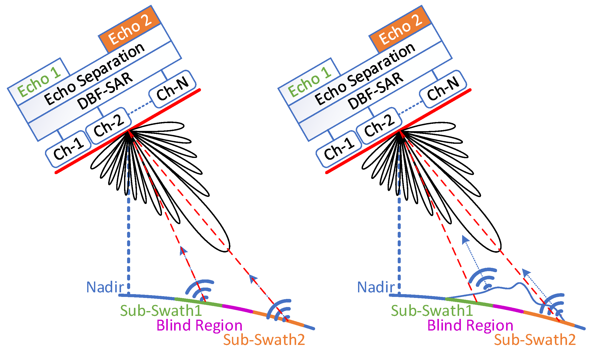
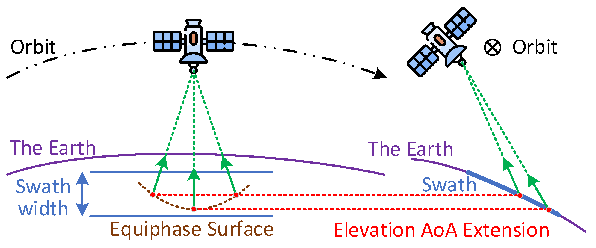
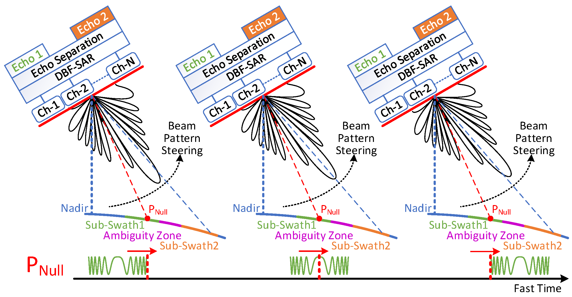
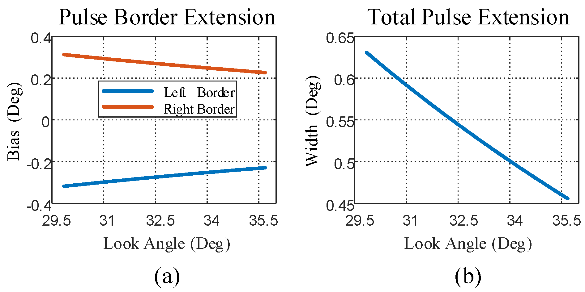
2. Existing Problems in the Traditional Scheme
3. Proposed Algorithm and Real-Time Processing Architecture
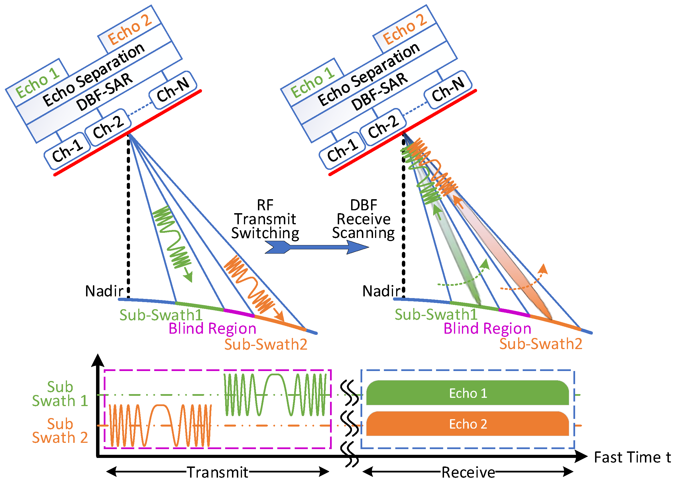
3.1. Principle and Algorithm Derivation
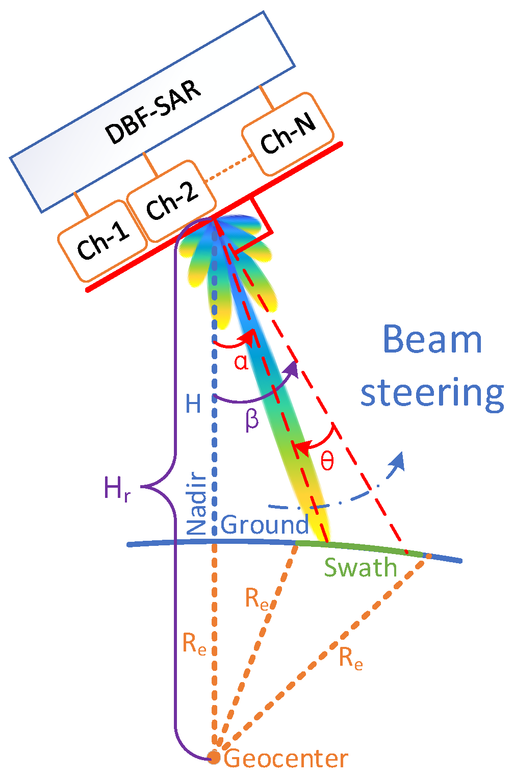
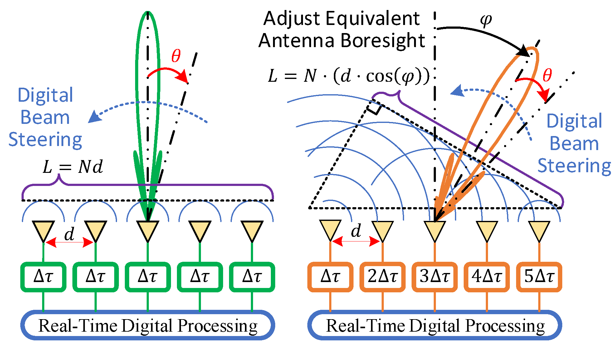
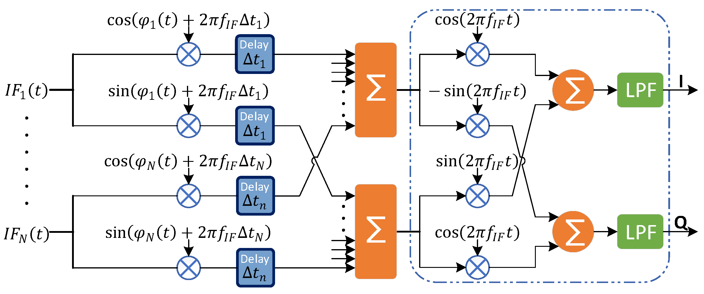
3.2. Digital Array Steering
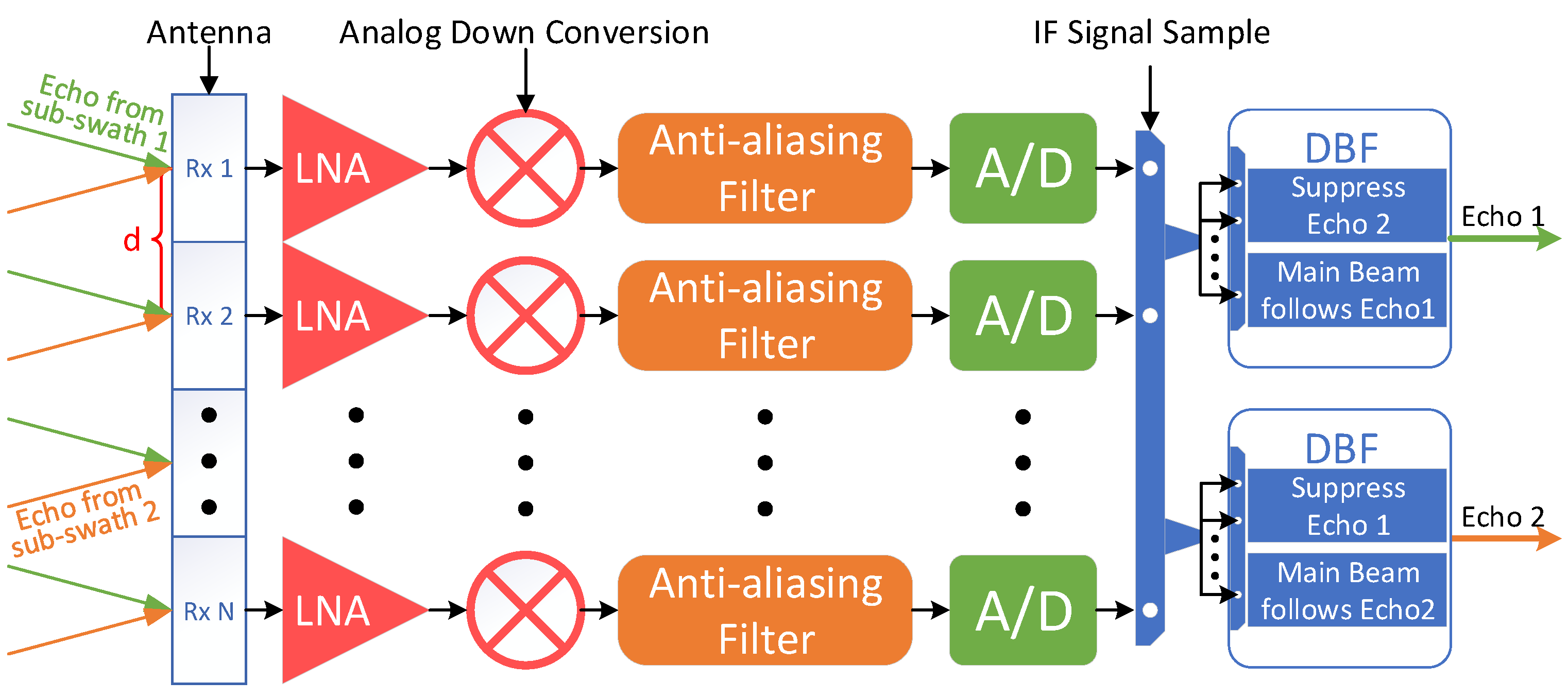
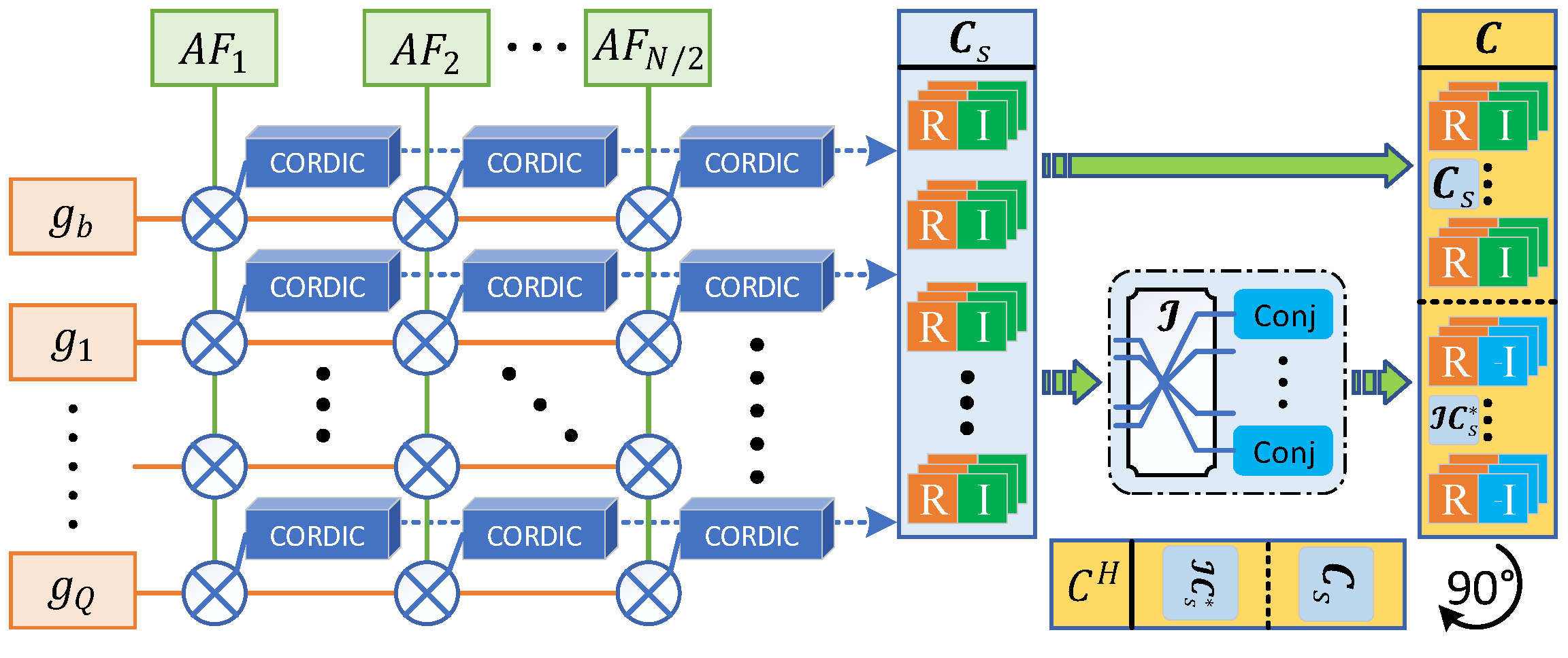
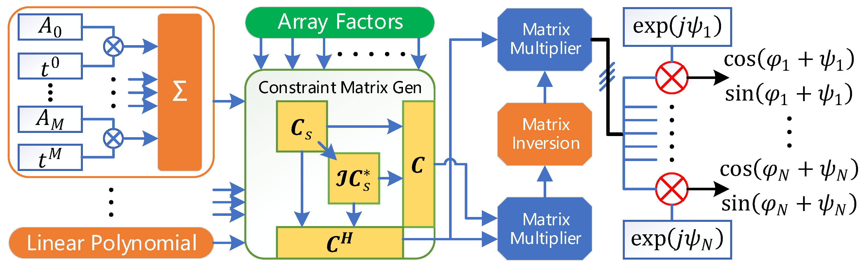
3.3. Real-Time Implementation
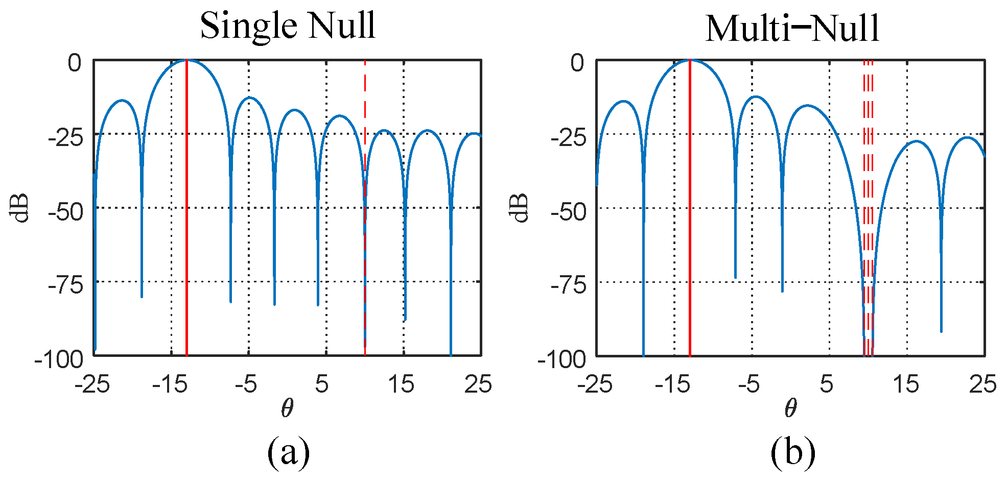
4. Simulation and Analysis
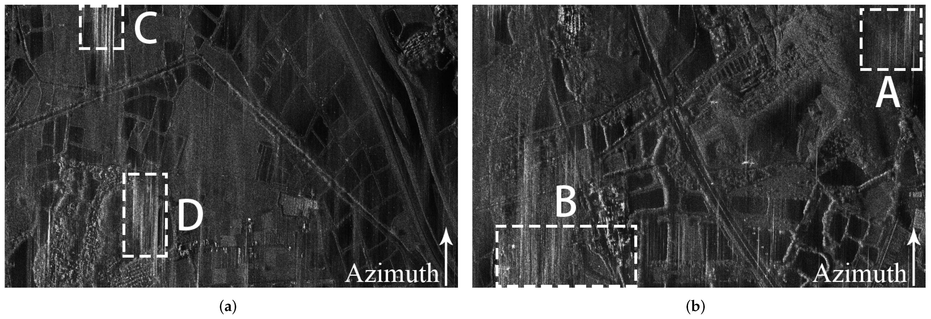
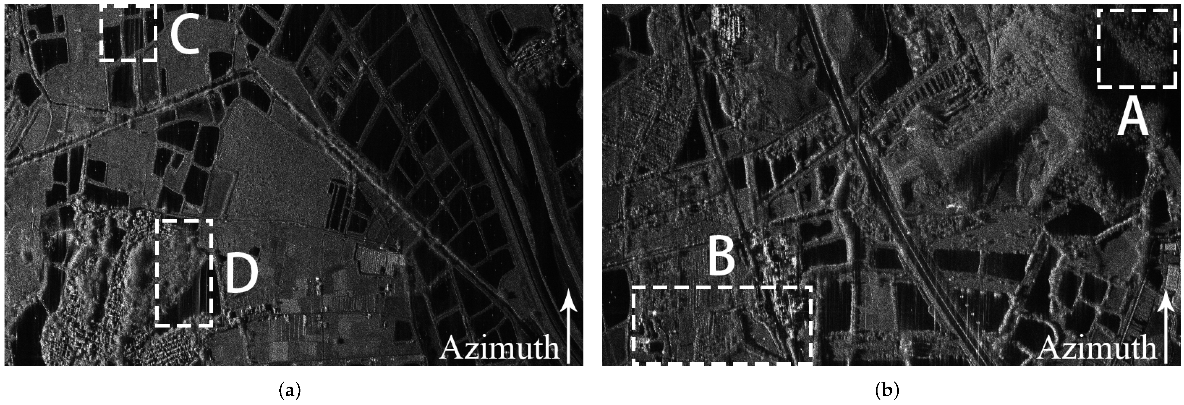
5. Experimental Results
6. Discussion
7. Conclusions
Author Contributions
Funding
Institutional Review Board Statement
Informed Consent Statement
Data Availability Statement
Conflicts of Interest
Appendix A. The Exchange Matrix
Appendix B. The Derivation Process of Equation (40)
References
- Huber, S.; de Almeida, F.Q.; Villano, M.; Younis, M.; Krieger, G.; Moreira, A. Tandem-L: A Technical Perspective on Future Spaceborne SAR Sensors for Earth Observation. IEEE Trans. Geosci. Remote Sens. 2018, 56, 4792–4807. [Google Scholar] [CrossRef] [Green Version]
- Adamiuk, G.; Gabele, M.; Loinger, A.; Heer, C.; Ludwig, M. Technology demonstration for future DBF based spaceborne SAR missions. In Proceedings of the EUSAR 2018, 12th European Conference on Synthetic Aperture Radar, Aachen, Germany, 4–7 June 2018; pp. 1–6. [Google Scholar]
- Bollian, T.; Osmanoglu, B.; Rincon, R.F.; Lee, S.K.; Fatoyinbo, T. MVDR Beamforming for RFI Suppression in EcoSAR data. In Proceedings of the EUSAR 2018, 12th European Conference on Synthetic Aperture Radar, Aachen, Germany, 4–7 June 2018; pp. 1–4. [Google Scholar]
- Freeman, A.; Johnson, W.T.K.; Huneycutt, B.; Jordan, R.; Hensley, S.; Siqueira, P.; Curlander, J. The “Myth” of the minimum SAR antenna area constraint. IEEE Trans. Geosci. Remote Sens. 2000, 38, 320–324. [Google Scholar] [CrossRef] [Green Version]
- Naftaly, U.; Levy-Nathansohn, R. Overview of the TECSAR Satellite Hardware and Mosaic Mode. IEEE Geosci. Remote Sens. Lett. 2008, 5, 423–426. [Google Scholar] [CrossRef]
- Raney, R.; Luscombe, A.; Langham, E.; Ahmed, S. RADARSAT (SAR imaging). Proc. IEEE 1991, 79, 839–849. [Google Scholar] [CrossRef]
- Gebert, N.; Krieger, G.; Moreira, A. Digital Beamforming on Receive: Techniques and Optimization Strategies for High-Resolution Wide-Swath SAR Imaging. IEEE Trans. Aerosp. Electron. Syst. 2009, 45, 564–592. [Google Scholar] [CrossRef] [Green Version]
- Suess, M.; Grafmueller, B.; Zahn, R. A novel high resolution, wide swath SAR system. In Proceedings of the IGARSS 2001, Scanning the Present and Resolving the Future, IEEE 2001 International Geoscience and Remote Sensing Symposium (Cat. No.01CH37217), Sydney, Australia, 9–13 July 2001; Volume 3, pp. 1013–1015. [Google Scholar]
- Zhou, Y.; Wang, W.; Chen, Z.; Wang, P.; Zhang, H.; Qiu, J.; Zhao, Q.; Deng, Y.; Zhang, Z.; Yu, W.; et al. Digital Beamforming Synthetic Aperture Radar (DBSAR): Experiments and Performance Analysis in Support of 16-Channel Airborne X-Band SAR Data. IEEE Trans. Geosci. Remote Sens. 2021, 59, 6784–6798. [Google Scholar] [CrossRef]
- Feng, F.; Li, S.; Yu, W.; Huang, P.; Xu, W. Echo Separation in Multidimensional Waveform Encoding SAR Remote Sensing Using an Advanced Null-Steering Beamformer. IEEE Trans. Geosci. Remote Sens. 2012, 50, 4157–4172. [Google Scholar] [CrossRef]
- Zhao, Q.; Zhang, Y.; Wang, W.; Deng, Y.; Yu, W.; Zhou, Y.; Wang, R. Echo Separation for Space–Time Waveform-Encoding SAR With Digital Scalloped Beamforming and Adaptive Multiple Null-Steering. IEEE Geosci. Remote Sens. Lett. 2021, 18, 92–96. [Google Scholar] [CrossRef]
- Krieger, G.; Gebert, N.; Moreira, A. Multidimensional Waveform Encoding: A New Digital Beamforming Technique for Synthetic Aperture Radar Remote Sensing. IEEE Trans. Geosci. Remote Sens. 2008, 46, 31–46. [Google Scholar] [CrossRef] [Green Version]
- Fischer, C.; Heer, C.; Werninghaus, R. X-Band HRWS demonstrator: Digital Beamforming test results. In Proceedings of the EUSAR 2012, 9th European Conference on Synthetic Aperture Radar, Nuremberg, Germany, 23–26 April 2012; pp. 1–4. [Google Scholar]
- Feng, F.; Dang, H.; Tan, X.; Li, G.; Li, C. An improved scheme of Digital Beam-Forming in elevation for spaceborne SAR. In Proceedings of the IET International Radar Conference 2013, Guilin, China, 14–16 April 2013; pp. 1–6. [Google Scholar]
- Younis, M.; Rommel, T.; Bordoni, F.; Krieger, G.; Moreira, A. On the Pulse Extension Loss in Digital Beamforming SAR. IEEE Geosci. Remote Sens. Lett. 2015, 12, 1436–1440. [Google Scholar] [CrossRef]
- Wang, W.; Wang, R.; Deng, Y.; Balz, T.; Hong, F.; Xu, W. An Improved Processing Scheme of Digital Beam-Forming in Elevation for Reducing Resource Occupation. IEEE Geosci. Remote Sens. Lett. 2016, 13, 309–313. [Google Scholar] [CrossRef]
- Qiu, J.; Zhang, Z.; Wang, R.; Wang, P.; Zhang, H.; Du, J.; Wang, W.; Chen, Z.; Zhou, Y.; Jia, H.; et al. A Novel Weight Generator in Real-Time Processing Architecture of DBF-SAR. IEEE Trans. Geosci. Remote Sens. 2021. [Google Scholar] [CrossRef]
- Zhao, Q.; Zhang, Y.; Wang, W.; Liu, K.; Deng, Y.; Zhang, H.; Wang, Y.; Zhou, Y.; Wang, R. On the Frequency Dispersion in DBF SAR and Digital Scalloped Beamforming. IEEE Trans. Geosci. Remote Sens. 2020, 58, 3619–3632. [Google Scholar] [CrossRef]
- Van Trees, H.L. Optimum Array Processing: Part IV of Detection, Estimation, and Modulation Theory; John Wiley & Sons, Inc.: New York, NY, USA, 2002. [Google Scholar]
- Mizzoni, R.; Capece, P.; Contu, S.; Meschini, A.; Ivagnes, M.; Rosati, G. Antennas for observation, exploration and navigation in ThalesAleniaSpace-Italia: Past and present challenges. In Proceedings of the 2017 11th European Conference on Antennas and Propagation (EUCAP), Paris, France, 19–24 March 2017; pp. 1516–1520. [Google Scholar] [CrossRef]
- Volder, J.E. The CORDIC Trigonometric Computing Technique. IRE Trans. Electron. Comput. 1959, EC-8, 330–334. [Google Scholar] [CrossRef]
- Irturk, A.; Benson, B.; Mirzaei, S.; Kastner, R. An FPGA Design Space Exploration Tool for Matrix Inversion Architectures. In Proceedings of the 2008 Symposium on Application Specific Processors(SASP), Anaheim, CA, USA, 8–9 June 2008; pp. 42–47. [Google Scholar] [CrossRef] [Green Version]
- de Almeida, F.Q.; Younis, M.; Krieger, G.; Hensley, S.; Moreira, A. Investigation into the Weight Update Rate for Scan-On-Receive Beamforming. In Proceedings of the 2020 IEEE Radar Conference (RadarConf20), Florence, Italy, 21–25 September 2020; pp. 1–6. [Google Scholar] [CrossRef]
- Yang, T.; Lv, X.; Wang, Y.; Qian, J. Study on a Novel Multiple Elevation Beam Technique for HRWS SAR System. IEEE J. Sel. Top. Appl. Earth Obs. Remote Sens. 2015, 8, 5030–5039. [Google Scholar] [CrossRef]
- Echman, F.; Owall, V. A scalable pipelined complex valued matrix inversion architecture. In Proceedings of the 2005 IEEE International Symposium on Circuits and Systems (ISCAS), Kobe, Japan, 23–26 May 2005; Volume 5, pp. 4489–4492. [Google Scholar] [CrossRef]
- Ma, L.; Dickson, K.; McAllister, J.; McCanny, J. Modified givens rotations and their application to matrix inversion. In Proceedings of the 2008 IEEE International Conference on Acoustics, Speech and Signal Processing, Las Vegas, Nevada, USA, 30 March–4 April 2008; pp. 1437–1440. [Google Scholar] [CrossRef]
- Singh, A.K. Fast inversion of positive definite Hermitian matrices using real inverse operations. In Proceedings of the 2015 Annual IEEE India Conference (INDICON), New Delhi, India, 17–20 December 2015; pp. 1–3. [Google Scholar] [CrossRef]
- V, C.; Kuloor, R. Novel Architecture for Highly Hardware Efficient Implementation of Real Time Matrix Inversion Using Gauss Jordan Technique. In Proceedings of the 2010 IEEE Computer Society Annual Symposium on VLSI, Lixouri, Greece, 5–7 July 2010; pp. 294–298. [Google Scholar] [CrossRef]
- Khan, F.A.; Ashraf, R.A.; Abbasi, Q.H.; Nasir, A.A. Resource efficient parallel architectures for linear matrix algebra in real time adaptive control algorithms on reconfigurable logic. In Proceedings of the 2008 Second International Conference on Electrical Engineering, Lahore, Pakistan, 25–26 March 2008; pp. 1–9. [Google Scholar] [CrossRef]
- Rosado, A.; Iakymchuk, T.; Bataller, M.; Wegrzyn, M. Hardware-efficient matrix inversion algorithm for complex adaptive systems. In Proceedings of the 2012 19th IEEE International Conference on Electronics, Circuits, and Systems (ICECS 2012), Seville, Spain, 9–12 December 2012; pp. 41–44. [Google Scholar] [CrossRef]
- Hager, W.W. Updating the Inverse of a Matrix. SIAM Rev. 1989, 31, 221–239. [Google Scholar] [CrossRef]
- Hadizadeh, A.; Hashemi, M.; Labbaf, M.; Parniani, M. A Matrix-Inversion Technique for FPGA-Based Real-Time EMT Simulation of Power Converters. IEEE Trans. Ind. Electron. 2019, 66, 1224–1234. [Google Scholar] [CrossRef]


| Parameter | Value |
|---|---|
| Carrier Frequency | 9.6 GHz |
| Sample Rate | 1360 MHz |
| Transmit Signal Pulse width | 10 s |
| Transmit Window Duration | 50 s |
| Signal Bandwidth | 600 MHz |
| Orbit Height | 750 Km |
| Reference Earth Radius | 6,371,393 m |
| Antenna Height (Elevation) | 2 m |
| Antenna Length (Azimuth) | 12 m |
| Number of Elevation Channels | 24 |
| Width of Sub-Swaths (Slant Range) | 80 Km |
| Number of Sub-Swaths | 4 |
| Ideal Resolution (Slant Range) | 0.25 m |
| Ideal Resolution (Azimuth) | 6 m |
| Total Witdh of Swath (Slant Range) | 320 Km |
| Swath | PRF | Look Angle |
|---|---|---|
| 1 | 1400 | [, ] |
| 2 | 1400 | [, ] |
| 3 | 1400 | [, ] |
| 4 | 1400 | [, ] |
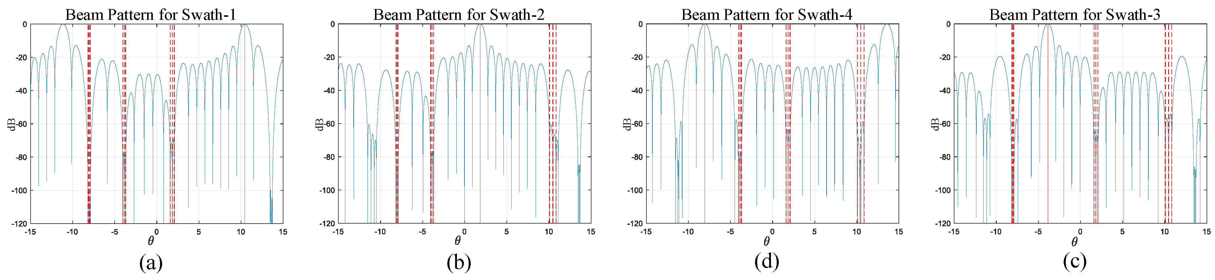
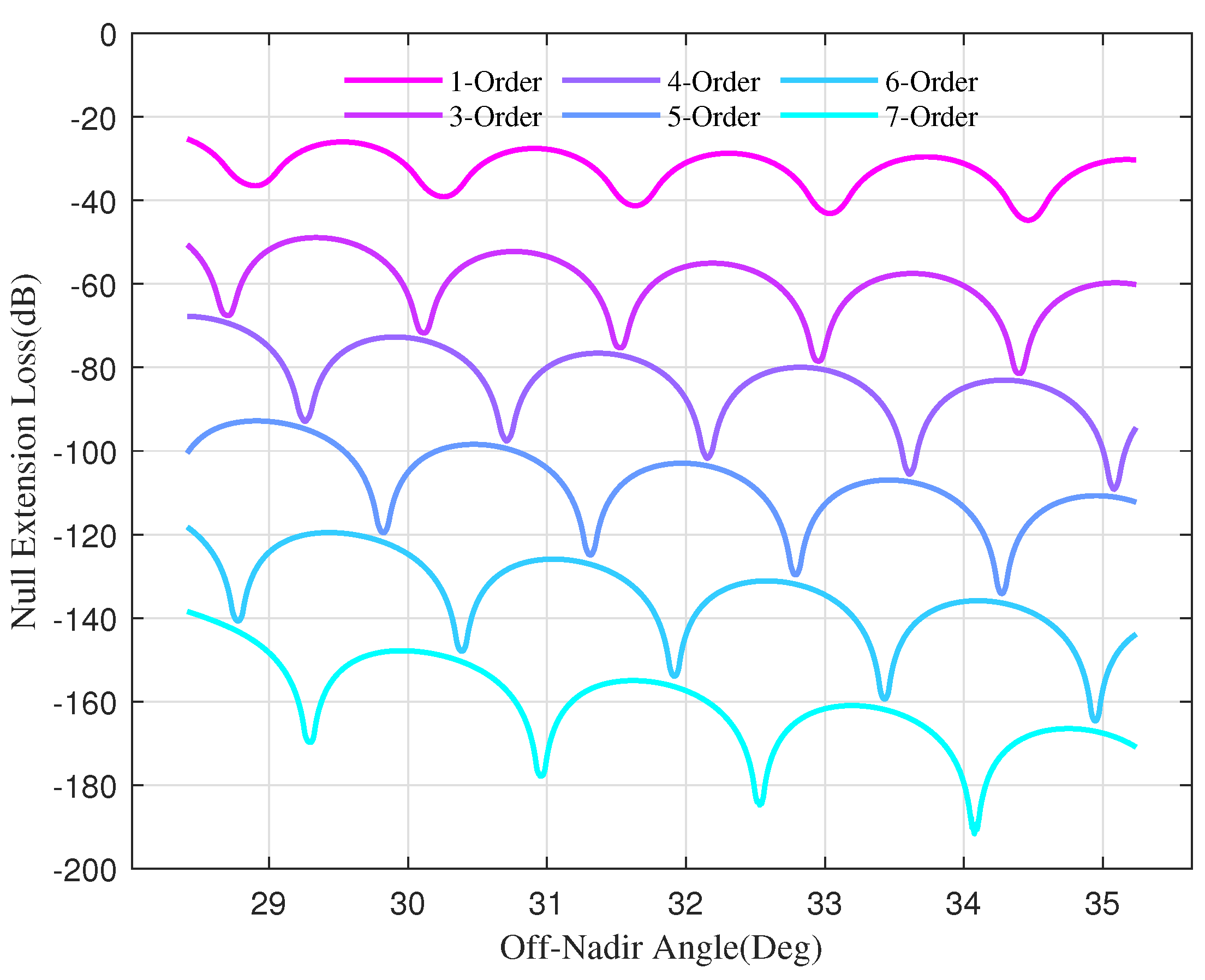
| Order | Swath-1 | Swath-2 | Swath-3 | Swath-4 |
|---|---|---|---|---|
| 1 | −32.8755 | −39.6801 | −43.2751 | −42.2908 |
| 3 | −59.8992 | −74.5834 | −84.3336 | −88.5442 |
| 4 | −83.4885 | −103.428 | −113.926 | −120.941 |
| 5 | −107.704 | −130.451 | −145.837 | −153.970 |
| 6 | −134.845 | −161.980 | −178.161 | −188.434 |
| 7 | −161.084 | −188.833 | −182.322 | −184.303 |
| Parameter | Value |
|---|---|
| Carrier frequency | 9.6 GHz |
| Velocity | 70 m/s |
| Height | 4200 m |
| Incident angle | |
| Signal bandwidth | 500 MHz |
| Sampling frequency | 1200 MHz |
| Signal pulse duration | 10 s |
| Number of elevation channels | 16 |
Publisher’s Note: MDPI stays neutral with regard to jurisdictional claims in published maps and institutional affiliations. |
© 2022 by the authors. Licensee MDPI, Basel, Switzerland. This article is an open access article distributed under the terms and conditions of the Creative Commons Attribution (CC BY) license (https://creativecommons.org/licenses/by/4.0/).
Share and Cite
Qiu, J.; Zhang, Z.; Chen, Z.; Han, S.; Wang, W.; Wen, Y.; Meng, X.; Fan, H. A Novel Real-Time Echo Separation Processing Architecture for Space–Time Waveform-Encoding SAR Based on Elevation Digital Beamforming. Remote Sens. 2022, 14, 213. https://0-doi-org.brum.beds.ac.uk/10.3390/rs14010213
Qiu J, Zhang Z, Chen Z, Han S, Wang W, Wen Y, Meng X, Fan H. A Novel Real-Time Echo Separation Processing Architecture for Space–Time Waveform-Encoding SAR Based on Elevation Digital Beamforming. Remote Sensing. 2022; 14(1):213. https://0-doi-org.brum.beds.ac.uk/10.3390/rs14010213
Chicago/Turabian StyleQiu, Jinsong, Zhimin Zhang, Zhen Chen, Shuo Han, Wei Wang, Yuhao Wen, Xiangrui Meng, and Huaitao Fan. 2022. "A Novel Real-Time Echo Separation Processing Architecture for Space–Time Waveform-Encoding SAR Based on Elevation Digital Beamforming" Remote Sensing 14, no. 1: 213. https://0-doi-org.brum.beds.ac.uk/10.3390/rs14010213