
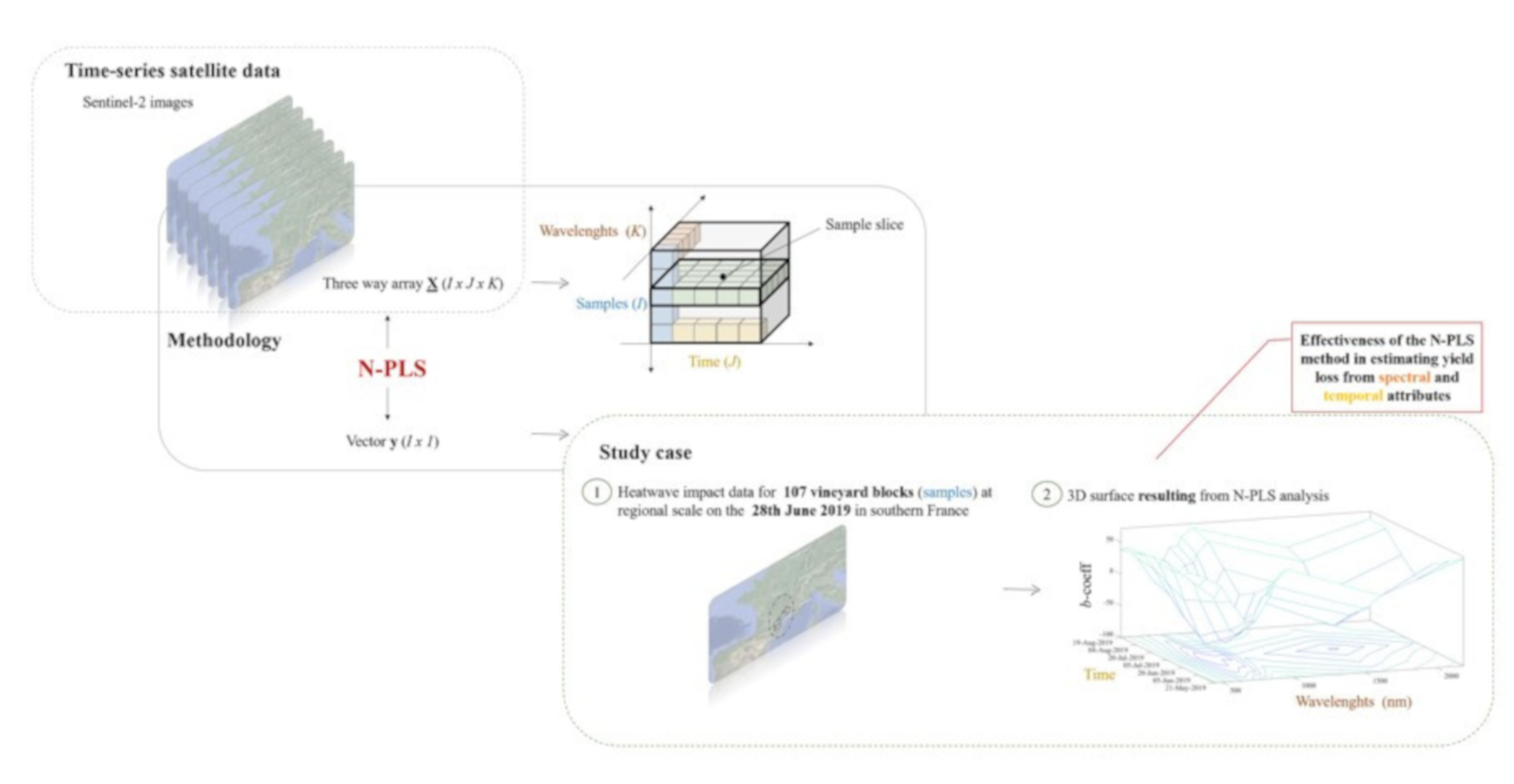
Potential of Multiway PLS (N-PLS) Regression Method to Analyse Time-Series of Multispectral Images: A Case Study in Agriculture


Abstract
:
1. Introduction
2. Materials and Methods
2.1. Type of Problem the N-Way Partial Least Squares Aims to Address in Remote Sensing
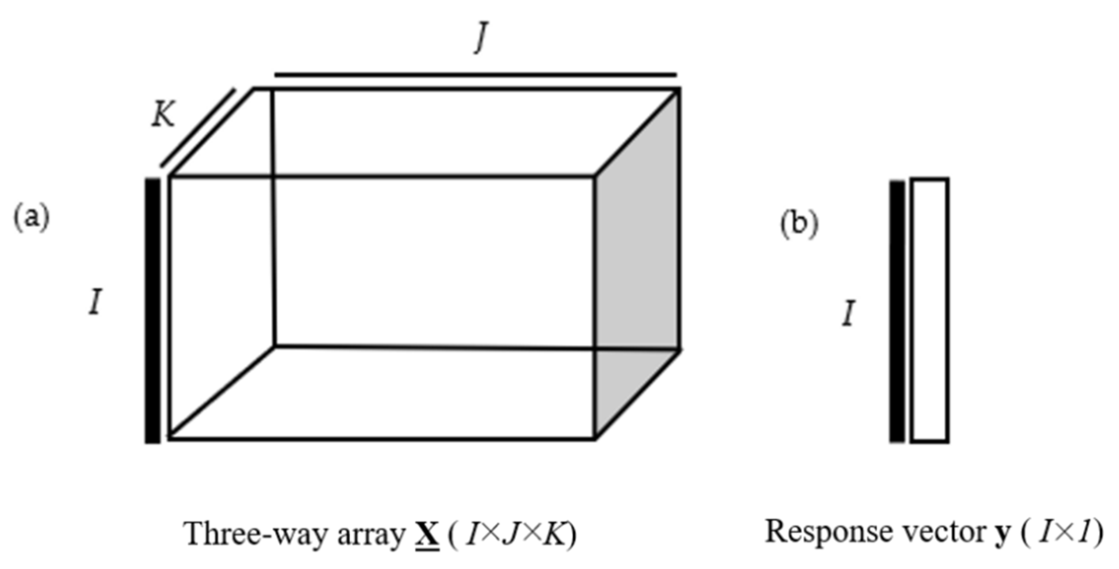
2.2. N-Way Partial Least Squares
- Compute the reshaped covariance matrix Ž = X (1 × JK).
- Define the first singular weight vectors and from : [, ] = svd(,1). From hence, store them as additional columns in separate weight arrays WJ = [… ] and WK […].
- Calculate S = XW.
- Calculate the regression coefficients regressing on S as b = (STS)−1 ST.
- Calculate the residuals = − Sb.
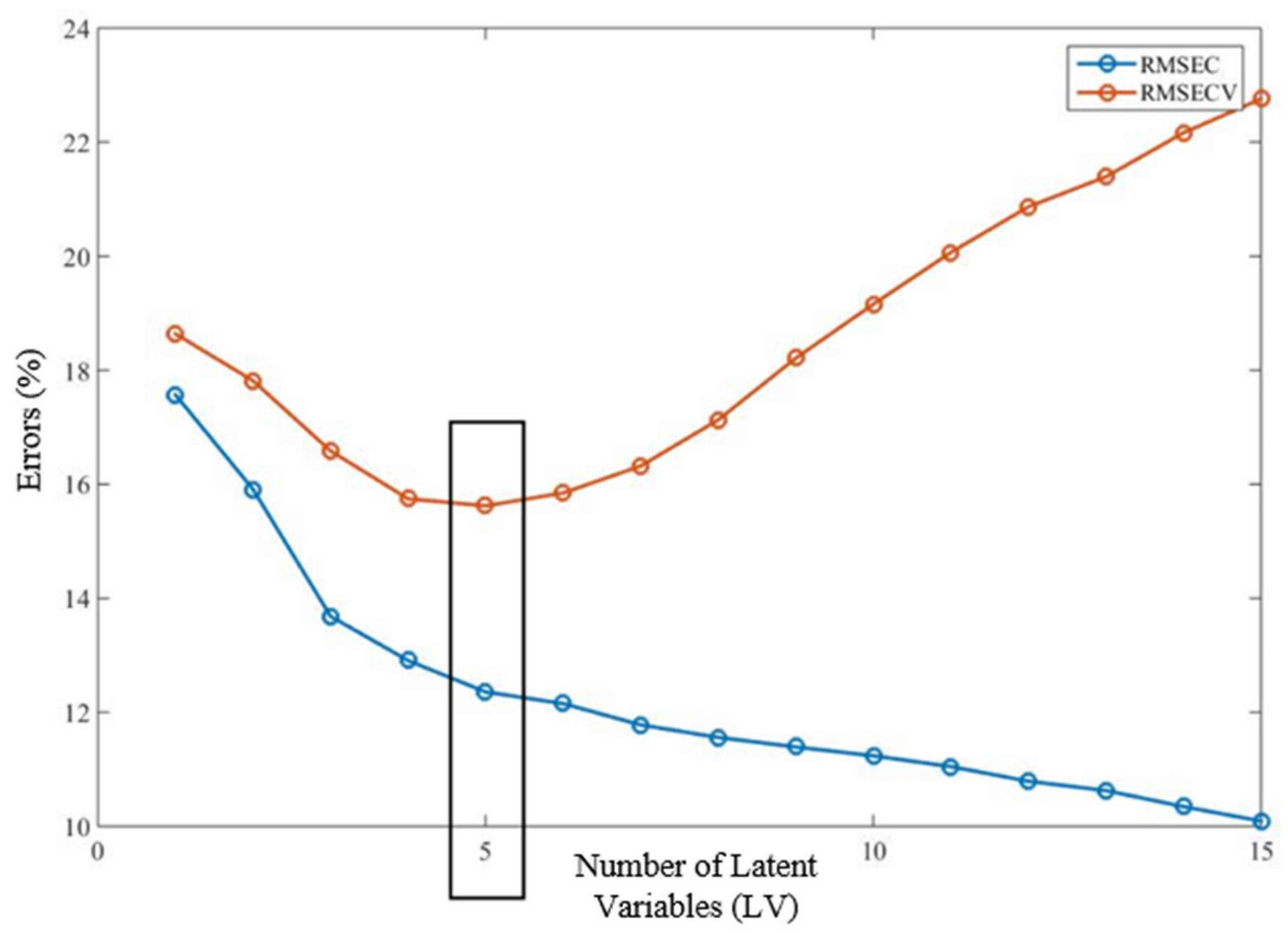
- Increase a to a + 1 and continue from step 1 to the appropriate description of . The inclusion of an additional latent variable (a + 1) in the model is terminated when the joint analysis of RMSEC (Root Mean Square Error of Calibration) and RMSECV (Root Mean Square Error of Cross-Validation) [30] indicates overfitting due to sampling variability.
2.3. Model Construction
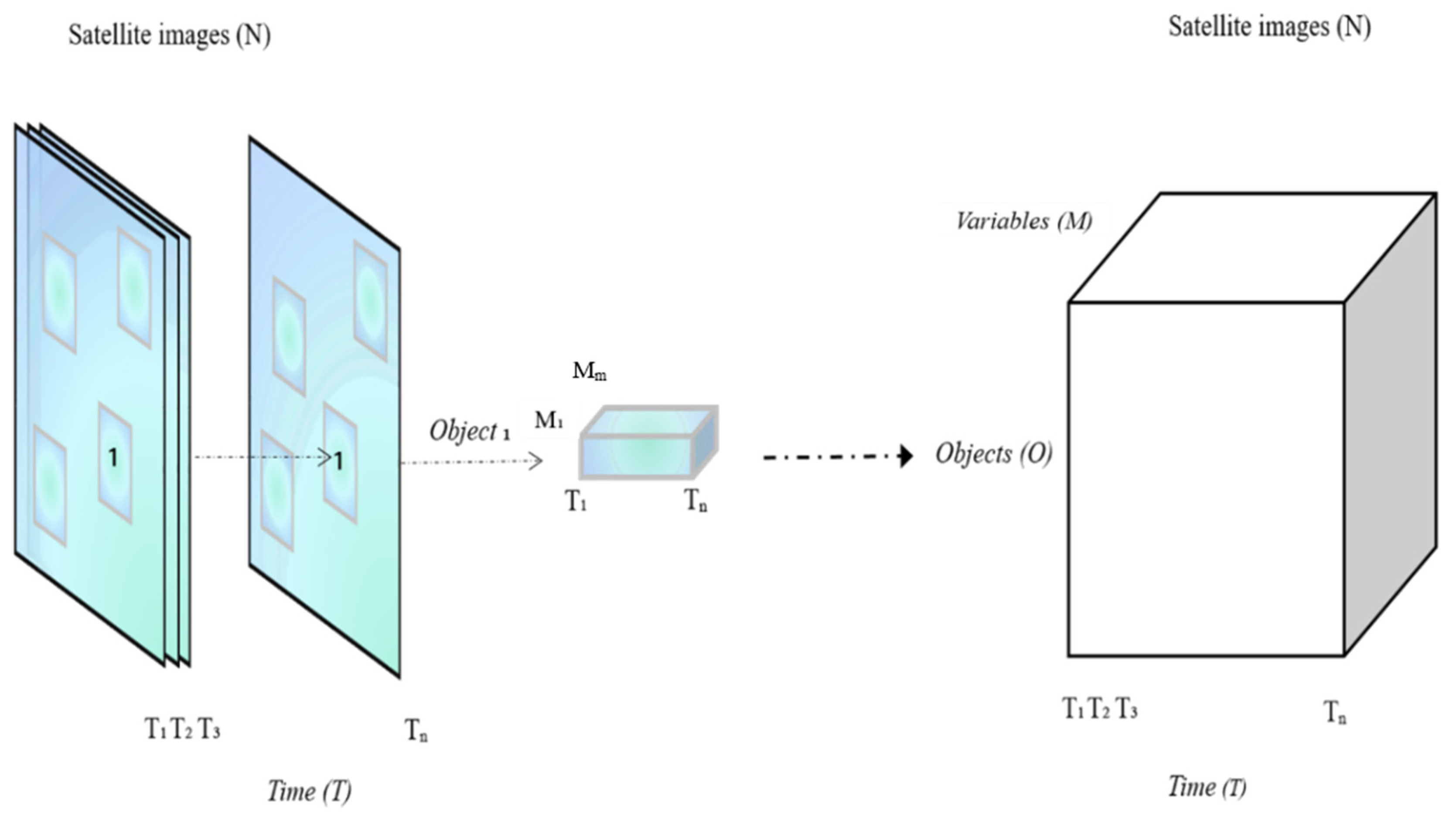
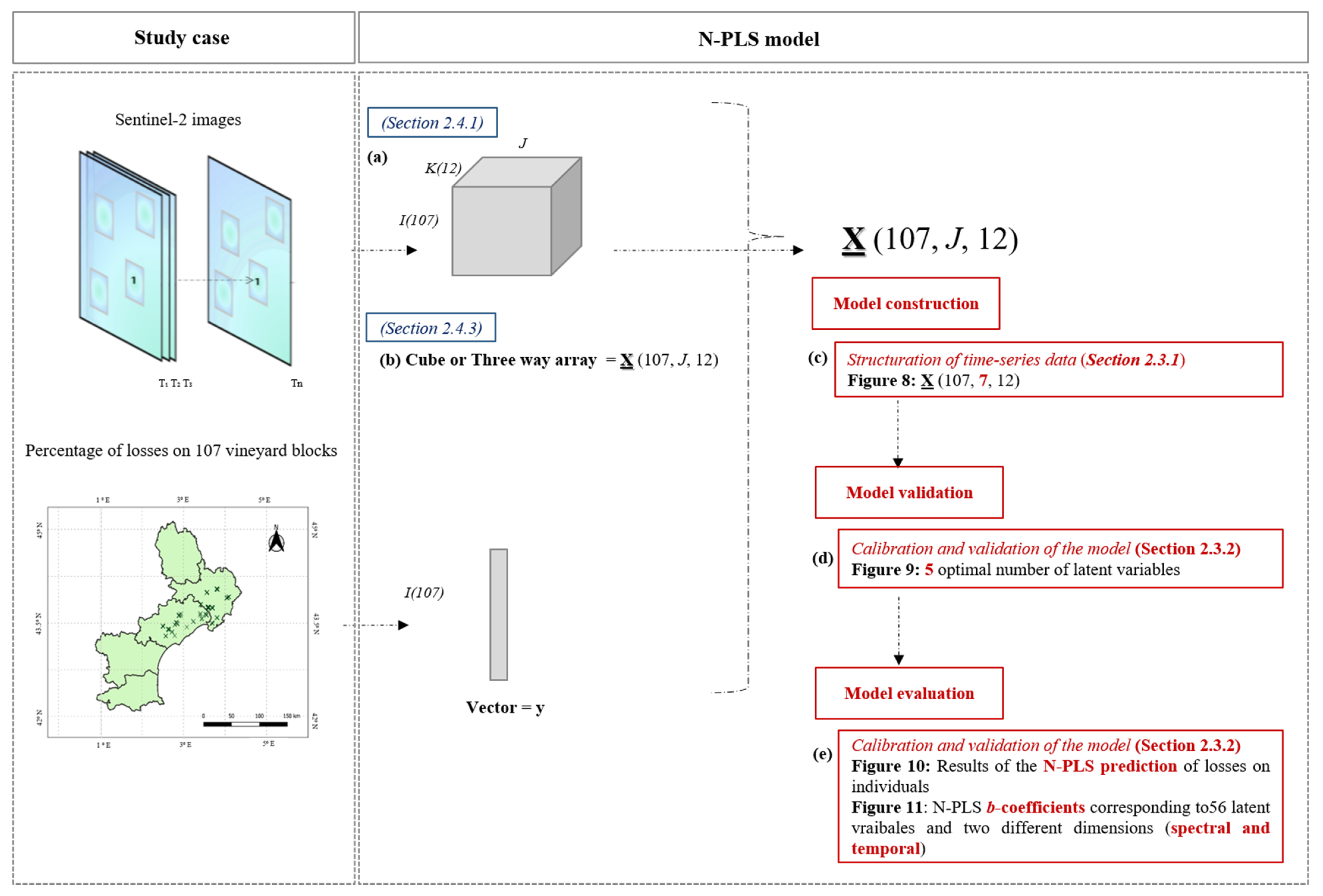
2.3.1. Structuration of Time-Series Data
2.3.2. Calibration and Validation of the Model
- The vector y was sorted in ascending order.
- After sorting, every fourth individual was placed in the validation set, the others retained in the calibration set.
2.4. Case-Study
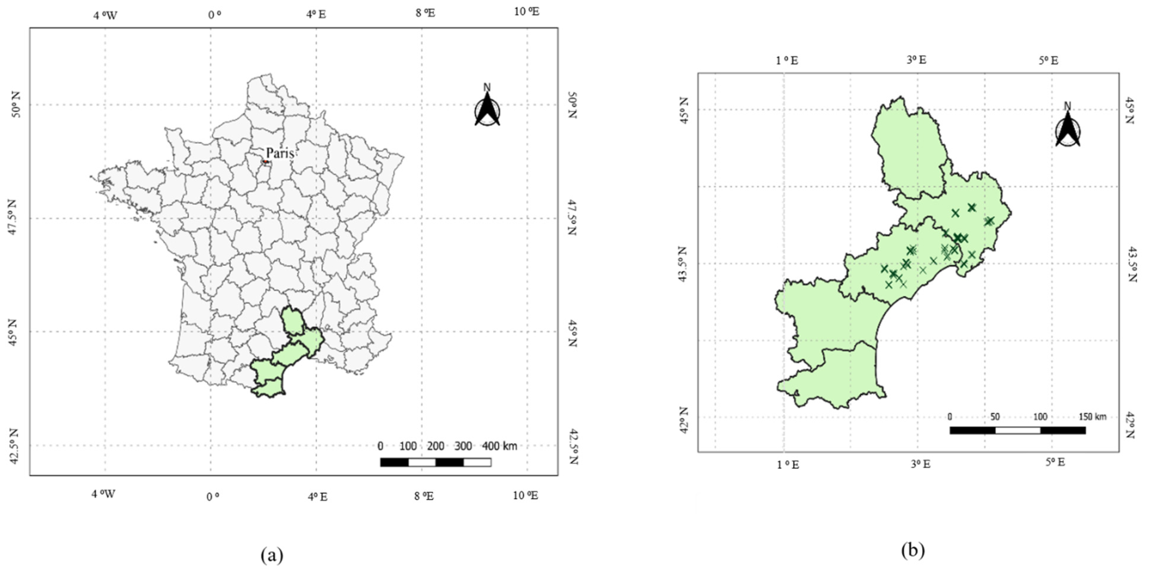
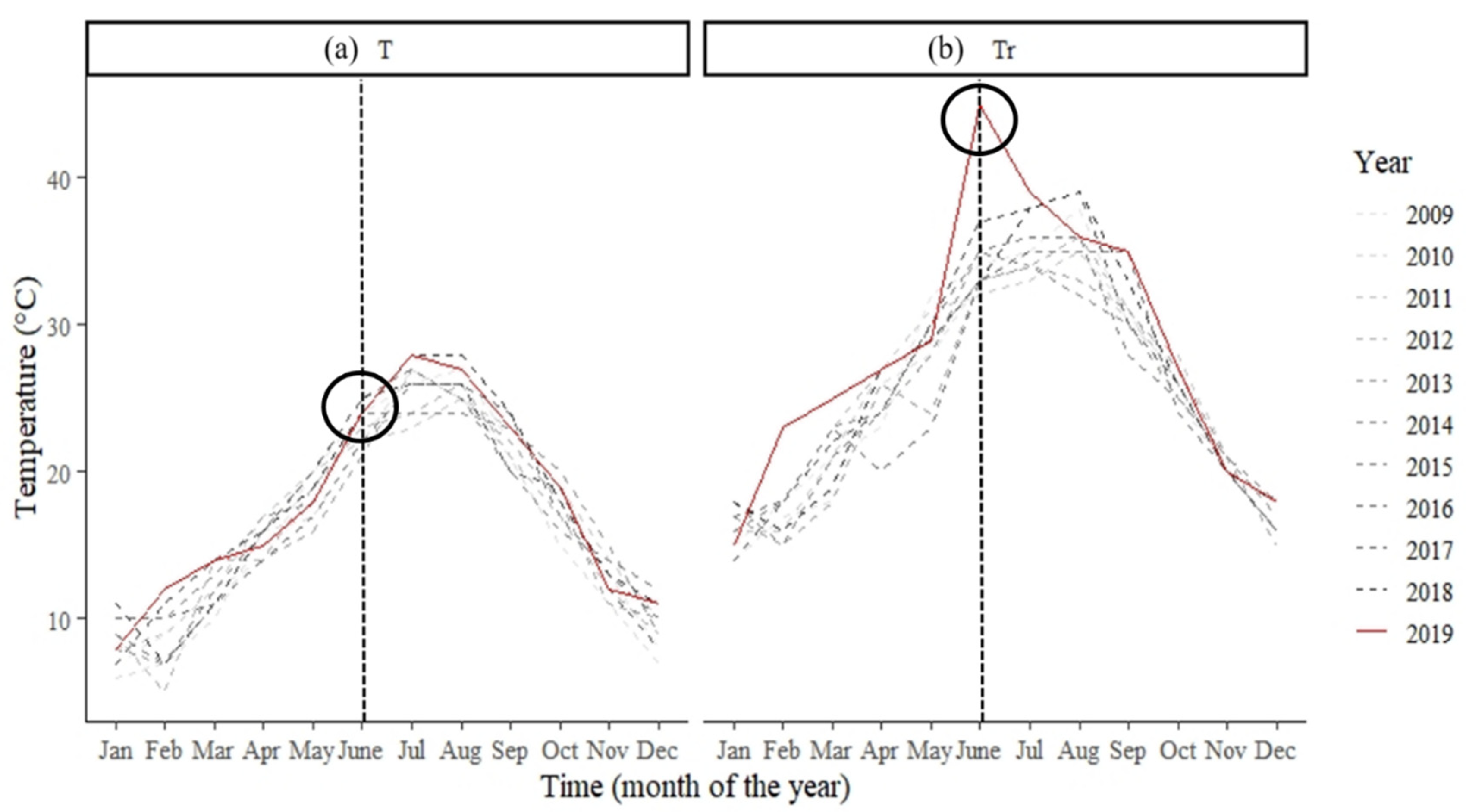
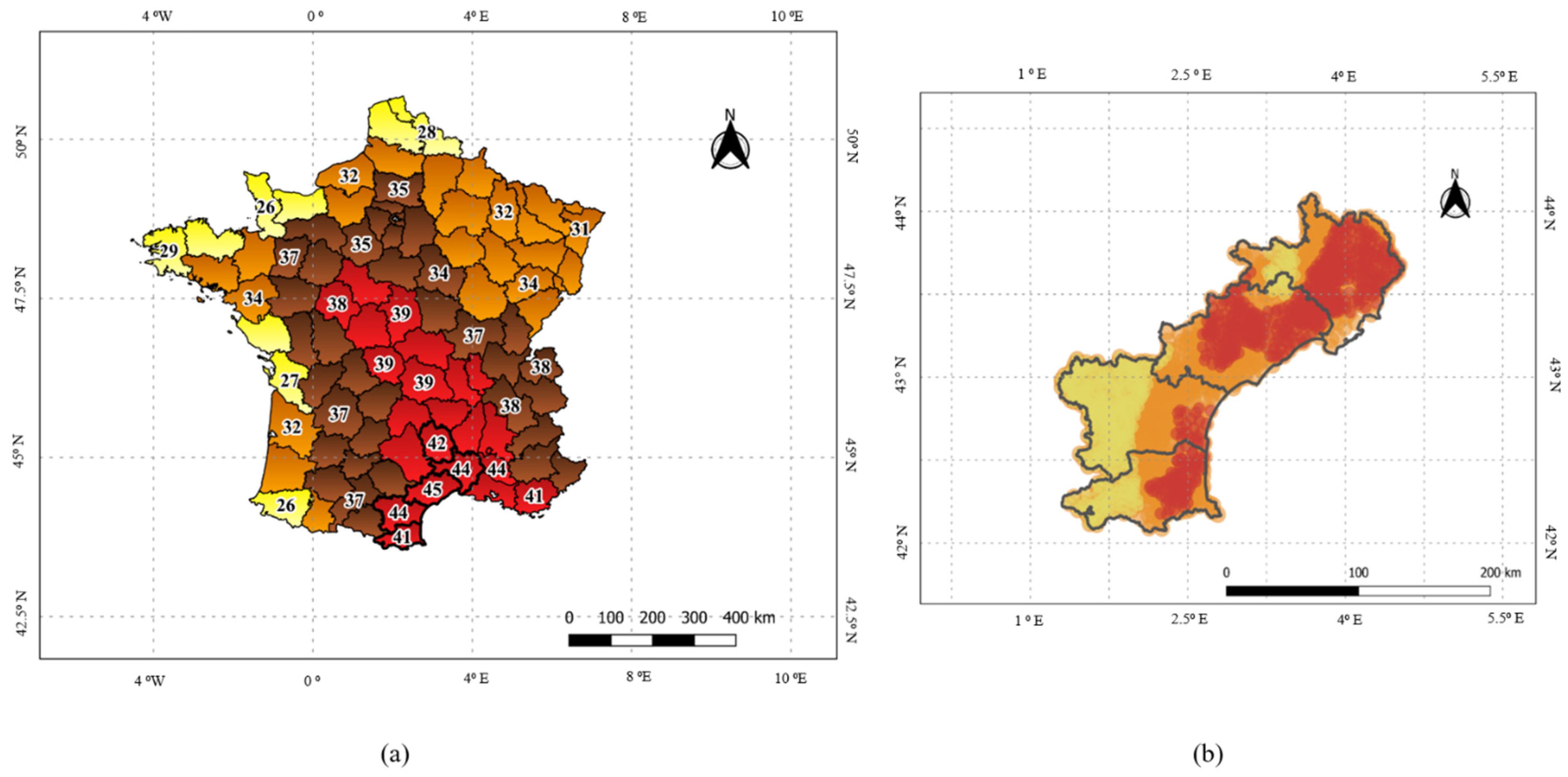
2.4.1. Study Area
2.4.2. Remote Sensing Data
Data Acquisition and Preprocessing
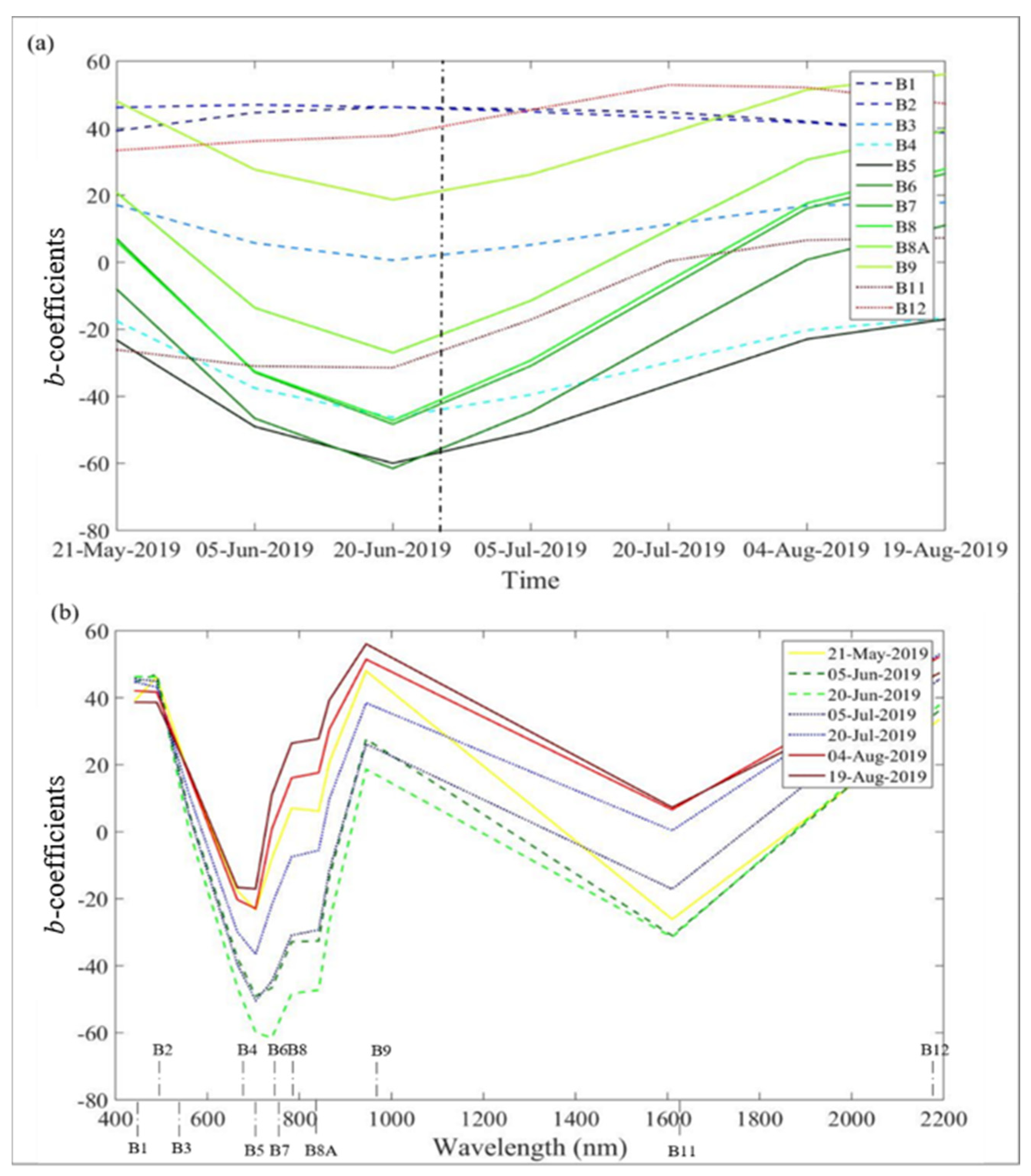
Spectral Bands
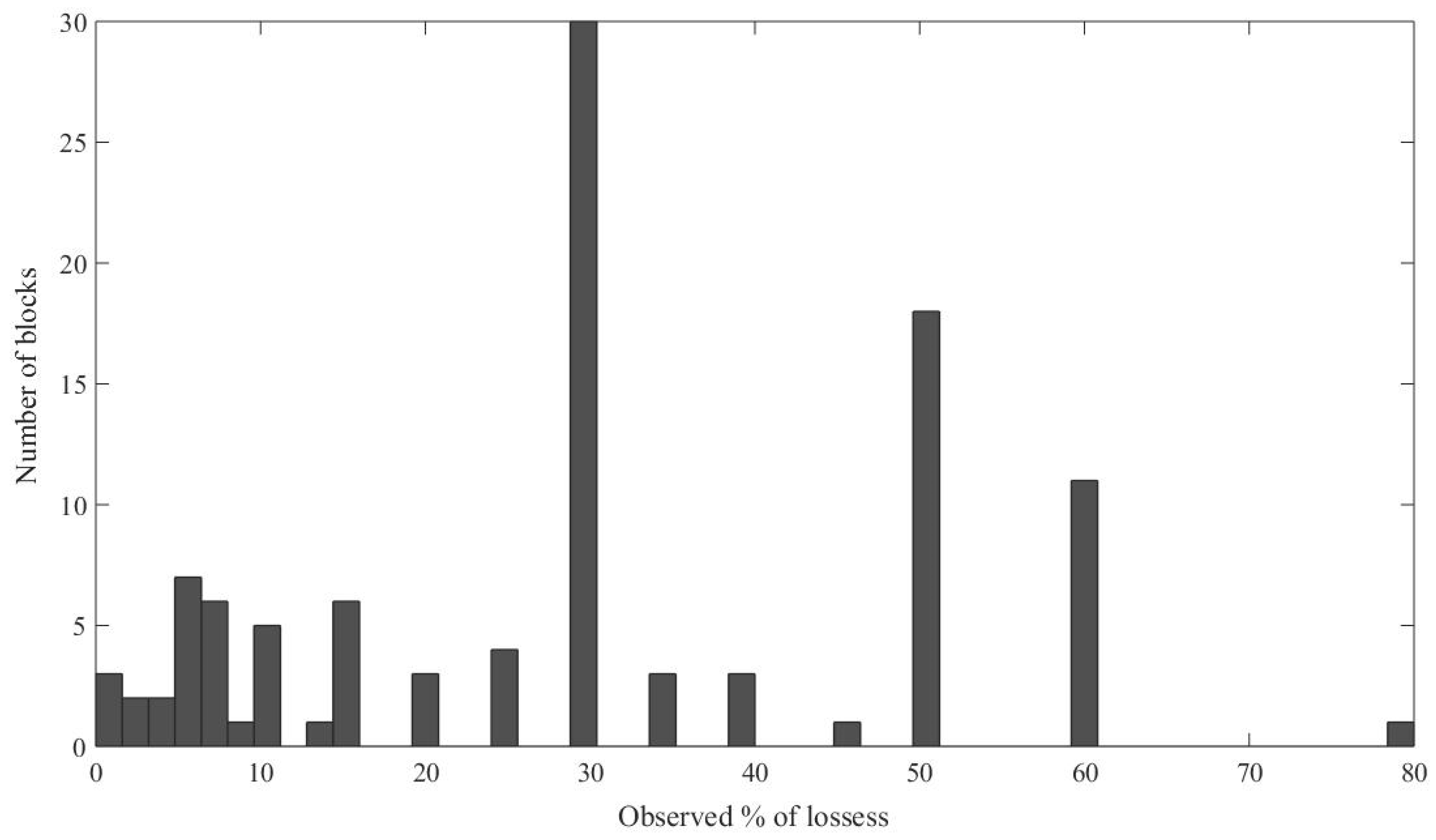
2.4.3. Ground-Truth Data
2.4.4. Modelling
Model Construction
- a cube X (107, J, 12) where the first dimension corresponds to the vineyard blocks (I), the second dimension corresponds to time (J), which is optimised during modelling, and the third dimension of the three-way array X corresponds to spectral bands (K) averaged for each field,
- a vector y (107), corresponding to the estimated percentage yield loss by the winegrowers from the 107 blocks.
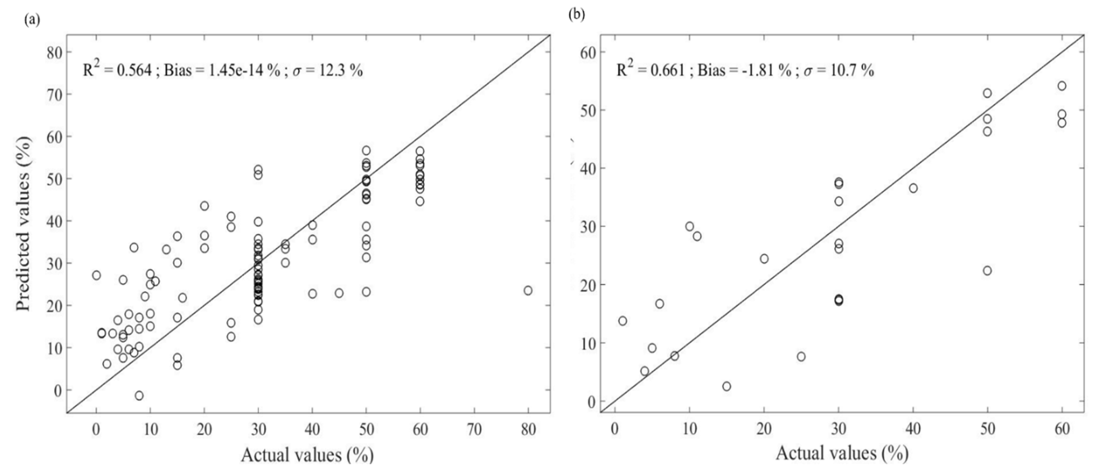
Model Validation
Model Evaluation
3. Results
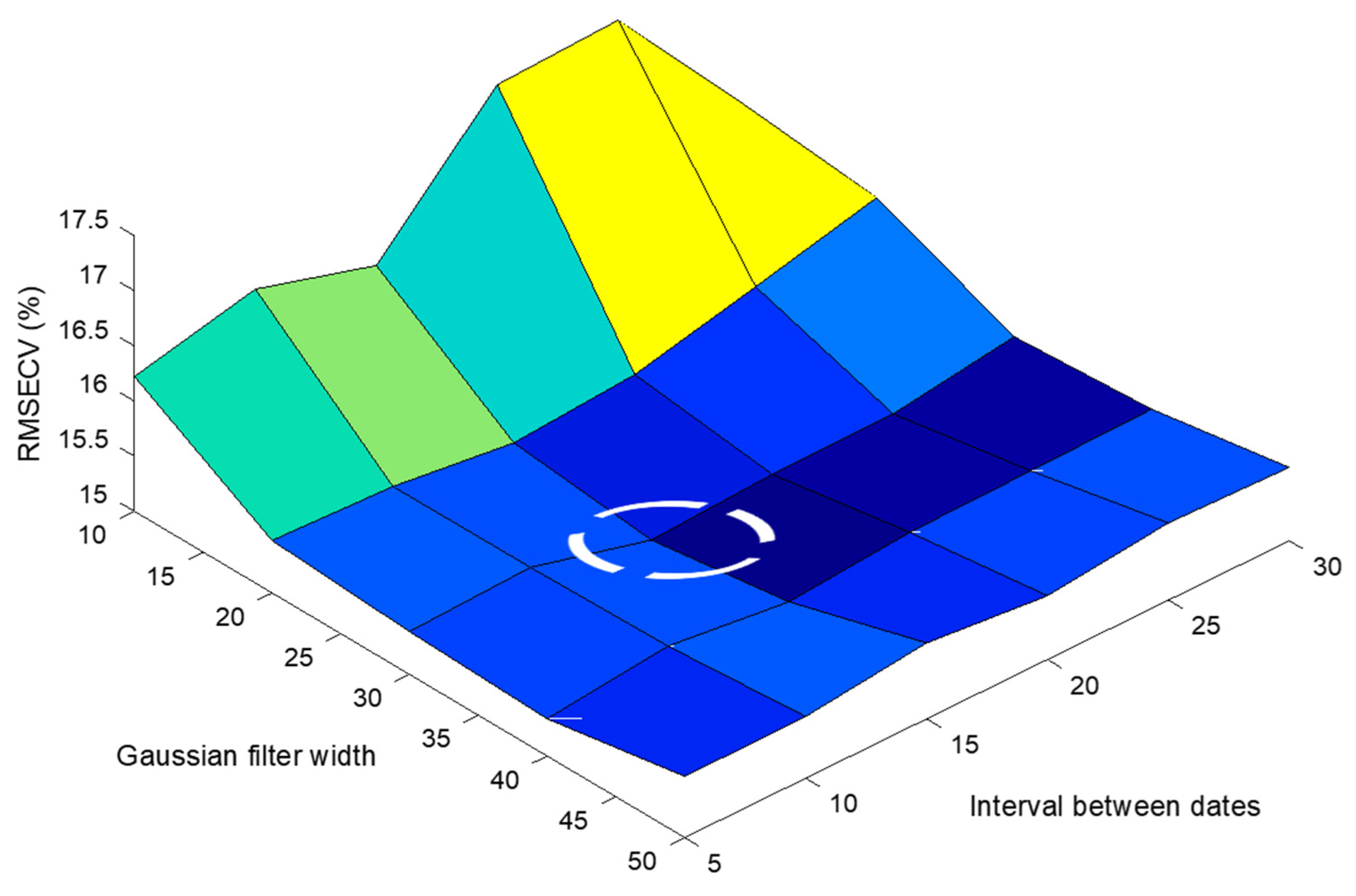
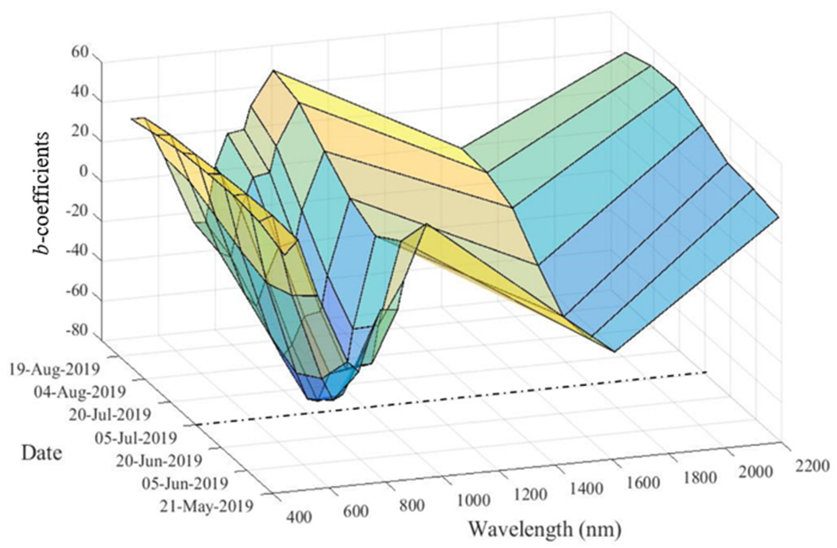
3.1. Optimisation of Model Parameters over the Study Site
3.2. Quality of the N-PLS Model
4. Discussion
5. Conclusions
Author Contributions
Funding
Acknowledgments
Conflicts of Interest
References
- Albanwan, H.; Qin, R. A Novel Spectrum Enhancement Technique for Multi-Temporal, Multi-Spectral Data Using Spatial-Temporal Filtering. ISPRS J. Photogramm. Remote Sens. 2018, 142, 51–63. [Google Scholar] [CrossRef]
- Bovolo, F.; Bruzzone, L. The Time Variable in Data Fusion: A Change Detection Perspective. IEEE Geosci. Remote Sens. Mag. 2015, 3, 8–26. [Google Scholar] [CrossRef]
- Mishra, S.; Shrivastava, P.; Dhurvey, P. Change Detection Techniques in Remote Sensing: A Review. IJWMCIS 2017, 4, 1–8. [Google Scholar] [CrossRef]
- Weiss, M.; Jacob, F.; Duveiller, G. Remote Sensing for Agricultural Applications: A Meta-Review. Remote Sens. Environ. 2020, 236, 111402. [Google Scholar] [CrossRef]
- Chen, Z.; Li, S.; Ren, J.; Gong, P.; Zhang, M.; Wang, L.; Xiao, S.; Jiang, D. Monitoring and Management of Agriculture with Remote Sensing. In Advances in Land Remote Sensing: System, Modeling, Inversion and Application; Liang, S., Ed.; Springer: Dordrecht, The Netherlands, 2008; pp. 397–421. ISBN 978-1-4020-6450-0. [Google Scholar]
- Venios, X.; Korkas, E.; Nisiotou, A.; Banilas, G. Grapevine Responses to Heat Stress and Global Warming. Plants 2020, 9, 1754. [Google Scholar] [CrossRef]
- Filella, I.; Serrano, L.; Serra, J.; Peñuelas, J. Evaluating Wheat Nitrogen Status with Canopy Reflectance Indices and Discriminant Analysis. Crop Sci. 1995, 35, 1400–1405. [Google Scholar] [CrossRef]
- Plant, R.E.; Munk, D.S.; Roberts, B.R.; Vargas, R.L.; Rains, D.W.; Travis, R.L.; Hutmacher, R.B. Relationships between remotely sensed reflectance data and cotton growth and yield. Trans. ASAE 2000, 43, 535–546. [Google Scholar] [CrossRef]
- Dorigo, W.A.; Zurita-Milla, R.; de Wit, A.J.W.; Brazile, J.; Singh, R.; Schaepman, M.E. A Review on Reflective Remote Sensing and Data Assimilation Techniques for Enhanced Agroecosystem Modeling. Int. J. App. Earth Obs. Geoinf. 2007, 9, 165–193. [Google Scholar] [CrossRef]
- Dayal, B.S.; MacGregor, J.F. Improved PLS algorithms. J. Chemom. 1997, 11, 73–85. [Google Scholar] [CrossRef]
- Phatak, A.; Jong, S.D. The Geometry of Partial Least Squares. J. Chemom. 1997, 11, 311–338. [Google Scholar] [CrossRef]
- Arenas-Garcia, J.; Camps-Valls, G. Feature Extraction from Remote Sensing Data Using Kernel Orthonormalized PLS. In Proceedings of the 2007 IEEE International Geoscience and Remote Sensing Symposium, Barcelona, Spain, 23–27 July 2007; pp. 258–261. [Google Scholar]
- Abdi, H.; Williams, L. Partial Least Squares Methods: Partial Least Squares Correlation and Partial Least Square Regression. Methods Mol. Biol. 2013, 930, 549–579. [Google Scholar] [CrossRef]
- Bishop, M.P. 3.1 Remote Sensing and GIScience in Geomorphology: Introduction and Overview. In Treatise on Geomorphology; Shroder, J.F., Ed.; Academic Press: San Diego, CA, USA, 2013; Volume 3, pp. 1–24. ISBN 978-0-08-088522-3. [Google Scholar]
- Mou, L.; Bruzzone, L.; Zhu, X.X. Learning Spectral-Spatial-Temporal Features via a Recurrent Convolutional Neural Network for Change Detection in Multispectral Imagery. IEEE Trans. Geosci. Remote Sens. 2019, 57, 924–935. [Google Scholar] [CrossRef] [Green Version]
- Henrion, R. N-Way Principal Component Analysis Theory, Algorithms and Applications. Chemom. Intell. Lab. Syst. 1994, 25, 1–23. [Google Scholar] [CrossRef]
- Bro, R. Multiway Calibration. Multilinear PLS. J. Chemom. 1996, 10, 47–61. [Google Scholar] [CrossRef]
- Li, S.; Song, W.; Fang, L.; Chen, Y.; Ghamisi, P.; Benediktsson, J.A. Deep Learning for Hyperspectral Image Classification: An Overview. IEEE Trans. Geosci. Remote Sens. 2019, 57, 6690–6709. [Google Scholar] [CrossRef] [Green Version]
- Smilde, A.K. Comments on Multilinear PLS. J. Chemom. 1997, 11, 367–377. [Google Scholar] [CrossRef]
- Hanafi, M.; Ouertani, S.S.; Boccard, J.; Mazerolles, G.; Rudaz, S. Multi-Way PLS Regression: Monotony Convergence of Tri-Linear PLS2 and Optimality of Parameters. CSDA 2015, 83, 129–139. [Google Scholar] [CrossRef]
- Sena, M.M.; Poppi, R.J. N-Way PLS Applied to Simultaneous Spectrophotometric Determination of Acetylsalicylic Acid, Paracetamol and Caffeine. J. Pharm. Biomed. 2004, 34, 27–34. [Google Scholar] [CrossRef]
- Coppi, R. An Introduction to Multiway Data and Their Analysis. CSDA 1994, 18, 3–13. [Google Scholar] [CrossRef]
- Cogato, A.; Pagay, V.; Marinello, F.; Meggio, F.; Grace, P.; De Antoni Migliorati, M. Assessing the Feasibility of Using Sentinel-2 Imagery to Quantify the Impact of Heatwaves on Irrigated Vineyards. Remote Sens. 2019, 11, 2869. [Google Scholar] [CrossRef] [Green Version]
- Zhao, Q.; Caiafa, C.F.; Mandic, D.P.; Zhang, L.; Ball, T.; Schulze-bonhage, A.; Cichocki, A. Multilinear Subspace Regression: An Orthogonal Tensor Decomposition Approach. In Proceedings of the 24th International Conference on Neural Information Processing Systems, Granada, Spain, 12–15 December 2011; Shawe-Taylor, J., Zemel, R.S., Bartlett, P.L., Pereira, F., Weinberger, K.Q., Eds.; Curran Associates, Inc.: New York, NY, USA, 2011. [Google Scholar]
- Abdi, H. Partial Least Squares (PLS) Regression. Wiley Interdiscip. Rev. Comput. Stat. 2010, 2, 97–106. [Google Scholar] [CrossRef]
- Hansen, P.M.; Jørgensen, J.R.; Thomsen, A. Predicting Grain Yield and Protein Content in Winter Wheat and Spring Barley Using Repeated Canopy Reflectance Measurements and Partial Least Squares Regression. J. Agric. Sci. 2002, 139, 307–318. [Google Scholar] [CrossRef]
- Bergant, K.; Kajfež-Bogataj, L. N–PLS Regression as Empirical Downscaling Tool in Climate Change Studies. Theor. Appl. Climatol. 2005, 81, 11–23. [Google Scholar] [CrossRef]
- Jong, S. de Regression Coefficients in Multilinear PLS. J. Chemom. 1998, 12, 77–81. [Google Scholar] [CrossRef]
- Bro, R.; Smilde, A.; Jong, S.D. On the Difference between Low-Rank and Subspace Approximation: Improved Model for Multi-Linear PLS Regression. Chemom. Intell. Lab. Syst. 2001, 58, 3–13. [Google Scholar] [CrossRef]
- Goodarzi, M.; Freitas, M.P. On the Use of PLS and N-PLS in MIA-QSAR: Azole Antifungals. Chemom. Intell. Lab. Syst. 2009, 96, 59–62. [Google Scholar] [CrossRef]
- Alam, M.S.; Islam, M.N.; Bal, A.; Karim, M.A. Hyperspectral Target Detection Using Gaussian Filter and Post-Processing. Opt. Lasers Eng. 2008, 46, 817–822. [Google Scholar] [CrossRef]
- Wang, Q.; Atkinson, P.M. Spatio-Temporal Fusion for Daily Sentinel-2 Images. Remote Sens. Environ. 2018, 204, 31–42. [Google Scholar] [CrossRef] [Green Version]
- Hird, J.N.; McDermid, G.J. Noise Reduction of NDVI Time Series: An Empirical Comparison of Selected Techniques. Remote Sens. Environ. 2009, 113, 248–258. [Google Scholar] [CrossRef]
- Fadzlillah, N.A.; Rohman, A.; Ismail, A.; Mustafa, S.; Khatib, A. Application of FTIR-ATR Spectroscopy Coupled with Multivariate Analysis for Rapid Estimation of Butter Adulteration. J. Oleo Sci. 2013, 62, 555–662. [Google Scholar] [CrossRef] [Green Version]
- Malegori, C.; Nascimento Marques, E.J.; de Freitas, S.T.; Pimentel, M.F.; Pasquini, C.; Casiraghi, E. Comparing the Analytical Performances of Micro-NIR and FT-NIR Spectrometers in the Evaluation of Acerola Fruit Quality, Using PLS and SVM Regression Algorithms. Talanta 2017, 165, 112–116. [Google Scholar] [CrossRef]
- Devaux, N.; Crestey, T.; Leroux, C.; Tisseyre, B. Potential of Sentinel-2 Satellite Images to Monitor Vine Fields Grown at a Territorial Scale. OENO One 2019, 53, 52–59. [Google Scholar] [CrossRef]
- Hollstein, A.; Segl, K.; Guanter, L.; Brell, M.; Enesco, M. Ready-to-Use Methods for the Detection of Clouds, Cirrus, Snow, Shadow, Water and Clear Sky Pixels in Sentinel-2 MSI Images. Remote Sens. 2016, 8, 666. [Google Scholar] [CrossRef] [Green Version]
- Knipling, E.B. Physical and Physiological Basis for the Reflectance of Visible and Near-Infrared Radiation from Vegetation. Remote Sens. Environ. 1970, 1, 155–159. [Google Scholar] [CrossRef]
- Segarra, J.; Buchaillot, M.L.; Araus, J.L.; Kefauver, S.C. Remote Sensing for Precision Agriculture: Sentinel-2 Improved Features and Applications. Agronomy 2020, 10, 641. [Google Scholar] [CrossRef]
- Seelig, H.-D.; Hoehn, A.; Stodieck, L.S.; Klaus, D.M.; Adams, W.W.; Emery, W.J. Plant Water Parameters and the Remote Sensing R 1300/R 1450 Leaf Water Index: Controlled Condition Dynamics during the Development of Water Deficit Stress. Irrig. Sci. 2009, 27, 357–365. [Google Scholar] [CrossRef]
- Laroche-Pinel, E.; Albughdadi, M.; Duthoit, S.; Chéret, V.; Rousseau, J.; Clenet, H. Understanding Vine Hyperspectral Signature through Different Irrigation Plans: A First Step to Monitor Vineyard Water Status. Remote Sens. 2021, 13, 536. [Google Scholar] [CrossRef]
- Easterday, K.; Kislik, C.; Dawson, T.E.; Hogan, S.; Kelly, M. Remotely Sensed Water Limitation in Vegetation: Insights from an Experiment with Unmanned Aerial Vehicles (UAVs). Remote Sens. 2019, 11, 1853. [Google Scholar] [CrossRef] [Green Version]
- Sims, D.A.; Gamon, J.A. Estimation of Vegetation Water Content and Photosynthetic Tissue Area from Spectral Reflectance: A Comparison of Indices Based on Liquid Water and Chlorophyll Absorption Features. Remote Sens. Environ. 2003, 84, 526–537. [Google Scholar] [CrossRef]
- Claverie, M.; Ju, J.; Masek, J.G.; Dungan, J.L.; Vermote, E.F.; Roger, J.-C.; Skakun, S.V.; Justice, C. The Harmonized Landsat and Sentinel-2 Surface Reflectance Data Set. Remote Sens. Environ. 2018, 219, 145–161. [Google Scholar] [CrossRef]
- Quintano, C.; Fernandez-manso, A.; Fernández-Manso, O. Combination of Landsat and Sentinel-2 MSI Data for Initial Assessing of Burn Severity. Int. J. App. Earth Obs. Geoinf. 2018, 64, 221–225. [Google Scholar] [CrossRef]


| Sentinel-2 Band | Central Wavelength (nm) | Bandwidth (nm) | Spatial Resolution (m) |
|---|---|---|---|
| Band 1–Aerosol | 442.7 | 21 | 60 |
| Band 2–Blue | 492.4 | 66 | 10 |
| Band 3–Green | 559.8 | 36 | 10 |
| Band 4–Red | 664.6 | 31 | 10 |
| Band 5–Vegetation Red Edge | 704.1 | 15 | 20 |
| Band 6–Vegetation Red Edge | 740.5 | 15 | 20 |
| Band 7–Vegetation Red Edge | 782.8 | 20 | 20 |
| Band 8–NIR | 832.8 | 106 | 10 |
| Band 8A–Vegetation Red Edge | 864.1 | 21 | 20 |
| Band 9–VNIR | 945.1 | 20 | 60 |
| Band 11–SWIR | 1613.1 | 91 | 20 |
| Band 12–SWIR | 2202.4 | 175 | 20 |
Publisher’s Note: MDPI stays neutral with regard to jurisdictional claims in published maps and institutional affiliations. |
© 2022 by the authors. Licensee MDPI, Basel, Switzerland. This article is an open access article distributed under the terms and conditions of the Creative Commons Attribution (CC BY) license (https://creativecommons.org/licenses/by/4.0/).
Share and Cite
Lopez-Fornieles, E.; Brunel, G.; Rancon, F.; Gaci, B.; Metz, M.; Devaux, N.; Taylor, J.; Tisseyre, B.; Roger, J.-M. Potential of Multiway PLS (N-PLS) Regression Method to Analyse Time-Series of Multispectral Images: A Case Study in Agriculture. Remote Sens. 2022, 14, 216. https://0-doi-org.brum.beds.ac.uk/10.3390/rs14010216
Lopez-Fornieles E, Brunel G, Rancon F, Gaci B, Metz M, Devaux N, Taylor J, Tisseyre B, Roger J-M. Potential of Multiway PLS (N-PLS) Regression Method to Analyse Time-Series of Multispectral Images: A Case Study in Agriculture. Remote Sensing. 2022; 14(1):216. https://0-doi-org.brum.beds.ac.uk/10.3390/rs14010216
Chicago/Turabian StyleLopez-Fornieles, Eva, Guilhem Brunel, Florian Rancon, Belal Gaci, Maxime Metz, Nicolas Devaux, James Taylor, Bruno Tisseyre, and Jean-Michel Roger. 2022. "Potential of Multiway PLS (N-PLS) Regression Method to Analyse Time-Series of Multispectral Images: A Case Study in Agriculture" Remote Sensing 14, no. 1: 216. https://0-doi-org.brum.beds.ac.uk/10.3390/rs14010216