
A Multiview Semantic Vegetation Index for Robust Estimation of Urban Vegetation Cover


1
The Institute for Sustainable Industries and Liveable Cities (ISILC), College of Engineering and Science, Victoria University, Melbourne, VIC 8001, Australia
2
School of Computing, Mathematics and Engineering, Charles Sturt University, Port Macquarie, NSW 2444, Australia
3
Applied Ecology Research Group, The Institute for Sustainable Industries and Liveable Cities (ISILC), College of Engineering and Science, Victoria University, Melbourne, VIC 8001, Australia
*
Author to whom correspondence should be addressed.
Remote Sens. 2022, 14(1), 228; https://0-doi-org.brum.beds.ac.uk/10.3390/rs14010228
Submission received: 16 October 2021
/
Revised: 10 December 2021
/
Accepted: 20 December 2021
/
Published: 5 January 2022
(This article belongs to the Special Issue Advances in Object and Activity Detection in Remote Sensing Imagery)
Abstract
:Urban vegetation growth is vital for developing sustainable and liveable cities in the contemporary era since it directly helps people’s health and well-being. Estimating vegetation cover and biomass is commonly done by calculating various vegetation indices for automated urban vegetation management and monitoring. However, most of these indices fail to capture robust estimation of vegetation cover due to their inherent focus on colour attributes with limited viewpoint and ignore seasonal changes. To solve this limitation, this article proposed a novel vegetation index called the Multiview Semantic Vegetation Index (MSVI), which is robust to color, viewpoint, and seasonal variations. Moreover, it can be applied directly to RGB images. This Multiview Semantic Vegetation Index (MSVI) is based on deep semantic segmentation and multiview field coverage and can be integrated into any vegetation management platform. This index has been tested on Google Street View (GSV) imagery of Wyndham City Council, Melbourne, Australia. The experiments and training achieved an overall pixel accuracy of 89.4% and 92.4% for FCN and U-Net, respectively. Thus, the MSVI can be a helpful instrument for analysing urban forestry and vegetation biomass since it provides an accurate and reliable objective method for assessing the plant cover at street level.
1. Introduction
The changing land use patterns and population growth have had a significant impact on the vegetation composition in the world [1,2,3] which is essential for better living conditions of city dwellers. As indicated by Wolf, K.L. [4], a city’s vegetation cover (i.e. street woods, lawns, etc.) has long been acknowledged as a key component of urban landscape planning. According to Appleyard [5], the instrumental role of street vegetation is to absorb airborne pollutants through carbon sequestration and oxygen production, to mitigate noise pollution in urban heat islands [6], and to reduce storm waters [7,8]. In addition, the life of vegetation generally raises the aesthetic evaluation of people in urban settings [9,10]. For this purpose, it is critical to document changes in vegetation so that land management professionals may work to improve the urban environment. Furthermore, changes in the type of land cover (such as building developments) have been found to have a strong correlation with the changes of vegetation in the urban environment.
Moreover, changes in an urban environment are generally very important. Food, energy, water, and land used by urban residents have a significant impact on the environment. Therefore, automated detection of vegetation cover is often done through calculations of various vegetation indexes [11] that hold important information regarding vegetation cover of a particular location. In the past, various algorithms were employed for the calculation of the vegetation index using various image modalities. However, existing approaches have highly focused on spectral analysis and color variations. For instance, Normalized Difference Vegetation Index (NDVI) tends to amplify atmospheric noise in the Near Infrared Reflectance (NIR) and Red bands and becomes very sensitive to background variation. Therefore, it does not work well for RGB images for street-level vegetation analysis. Remote sensing data collected from above by sensors (aircraft, space) misses the glimpse of urban flora at street level. Thus, profile views of urban greenery from the road level are insufficiently assessed, even though green indices derived from remotely sensed image data might help quantify urban greenery. There is a distinction between vegetation view through ground experience and the view captured by remote sensing systems [12]. Li et al. [13,14] discovered that people had unequal access to distinct types of urban greenery (street vegetation, private yard total vegetation, private yard trees and shrubs, and urban parks), providing the groundwork for subsequent research into urban greenery inequity.
On the other hand, RGB based vegetation indexes are prone to wrong estimations due to reliance on green color and ineffectiveness to capture seasonal variations. Rencai et al. [15] utilise the green view index (GVI) as a quantitative indicator to determine how much greenery can be seen by pedestrians and then apply an image segmentation algorithm to figure out how much greenery can be seen by pedestrians in street view images. Zhang et al. [16] used an extensive street view image data set, as well as a horizontal green view index (HGVI), to calculate the quantity of greenery visible from the street in their research. Long et al. [17] analysed 245 Chinese cities, calculating the GVI values of their central regions and comparing them to the overall GVI conditions of the respective cities. As a result, they discovered that more affluent and well-run cities have longer and greener streets. Several visual qualities of streets such as salient region saturation, visual entropy, a green view index, and a sky-openness index were measured by Cheng et al. [18].
Kendal et al. [19] used color threshold for extraction of the vegetation index. The technique proved to be promising, but only using color features for segmentation is not an efficient model as any clutter information in the image can match the vegetation color. Further, in recent years, Bawden et al. and Kattenborn et al [20,21] used convolutional neural network (CNN) for two studies: In the first approach, they used a CNN-based approach to train data acquired from unmanned aerial vehicle (UAV)-based high-resolution RGB imagery visual interpretation, a fine-grained map for two species of vegetation. In the second approach, they mapped species of trees or plants cover in different vegetation UAV RGB imagery. However, these approaches suffer due to reliance on color and specific image features and are unable to handle large variations in vegetation characteristics.
Recent advancements in deep learning have introduced a new level of accuracy in identifying objects of interest through semantic segmentation. Jonathan et al. [22] introduced a fully convolutional neural network (FCN), and Dvornik et al. [23] proposed BlitzNet for object segmentation. Yi et al. [24] constructed an instance aware based semantic segmentation model, which utilized the advantages of FCN for segmentation and classification. As a result of the development, the model was capable of simultaneously recognizing and segmenting the object instances. Liang-Chieh et al. [25] applied fully convolutional neural networks (FCN) to a multi-scale input image in order to achieve the required results.
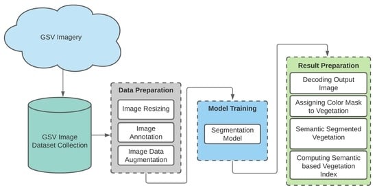
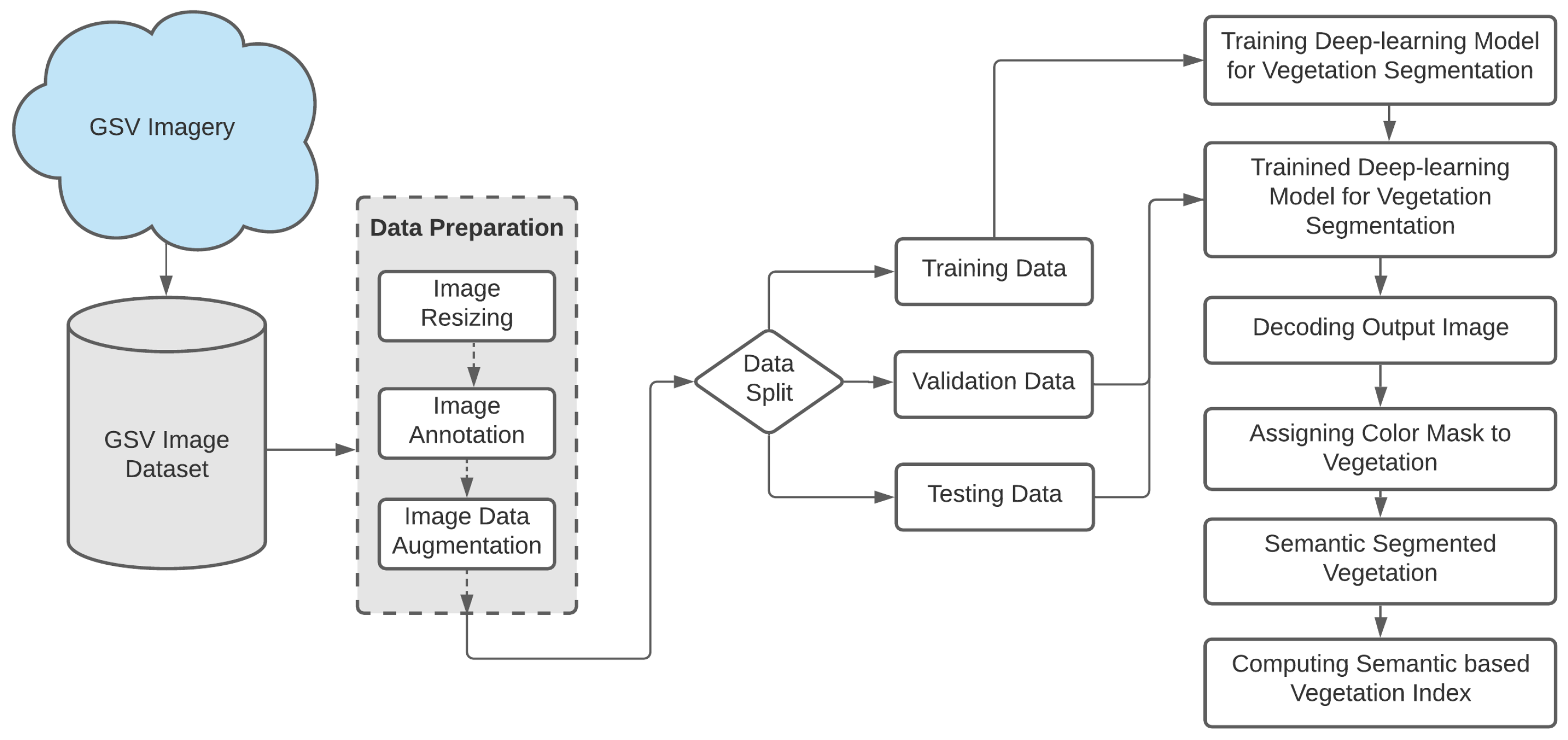
Motivated with the success of deep semantic segmentation, the conducted research proposes a semantic vegetation index (SVI) for RGB images with robustness against color changes and seasonal variations. To deal with the limitation of single image coverage, its extension, called multiview semantic vegetation index (MSVI), is also introduced, which can estimate vegetation cover from multiple views. The overall framework of this study is presented graphically in Figure 1.
The contribution: According to the literature, the semantic vegetation index (SVI) is one of the first approaches to integrate deep semantic segmentation into the process of vegetation index estimation. Although there are a variety of vegetation indexes in the literature, they are limited to a specific image modality and color feature, or they overlook essential flora semantic information. It makes them more susceptible to noise, resulting in erroneous estimation. The proposed index is robust to color and seasonal variations and works for any imaging modality. Furthermore, it can be extended to multiple views to expand exposure and reliable calculation. The segmentation approach is not claimed to have made a contribution in this study. Nonetheless, it compares many ways to determine which are the most appropriate for this aim.
The rest of the paper is organized as follows: Section 2 explains the materials and methods taken into account, Section 3 presents detailed information regarding the experiments and results achieved by the proposed methodology, Section 4 presents the comparative analysis with the previous work, Section 5 presents a detailed discussion of the proposed work, while Section 6 is the conclusion section of this paper.
2. Materials and Methods
2.1. Study Area
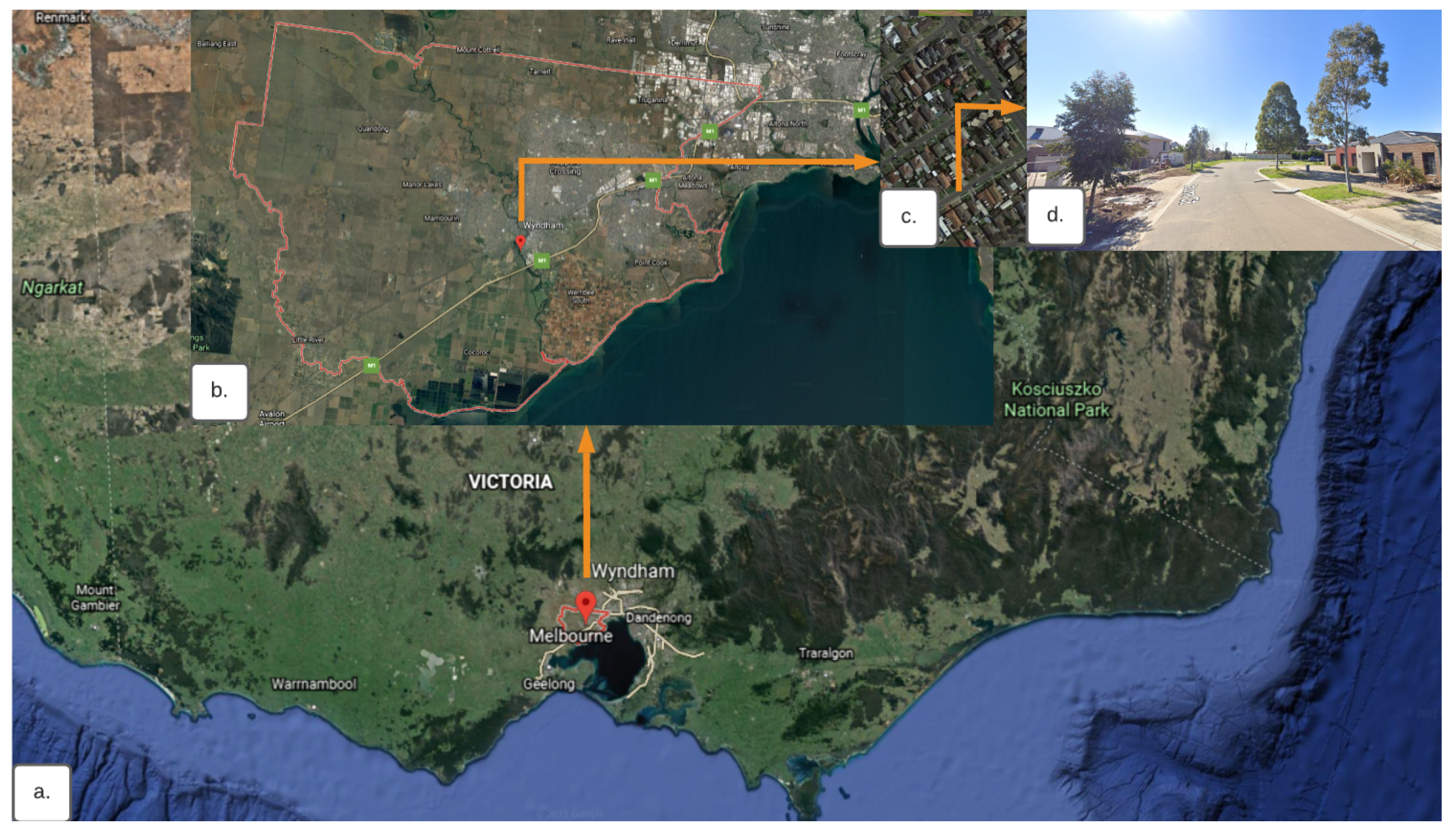
Figure 2 shows the municipal council of Wyndham (VIC, Australia), as the selected area for this study. It lies on the western outskirts of Melbourne (VIC, Australia) and covers an area of 542 km. According to the 2019 census, its estimated population is 270,478. Wyndham is the third fastest-growing council in the state of Victoria. The population of Wyndham is diverse, and the community development projects suggest that by 2031 more than 330,000 people are expected to come and live. Wyndham is home to 16 suburbs (Cocoroc, Eynesbury, Hoppers Crossing, Laverton North, Laverton RAAF, Little River, Mambourin, Mount Cottrell, Point Cook, Quandong, Tarneit, Truganina, Williams Landing, Manor Lakes, Quandong and Werribee South). The City Council of Wyndham is committed to improving residents’ environment and livelihoods. Every year, thousands of new trees and vegetation are planted in response to this commitment to increase Wyndham’s tree canopy cover through the street tree planting program [26].
2.2. Input Data Set/Google Street View Image Collection
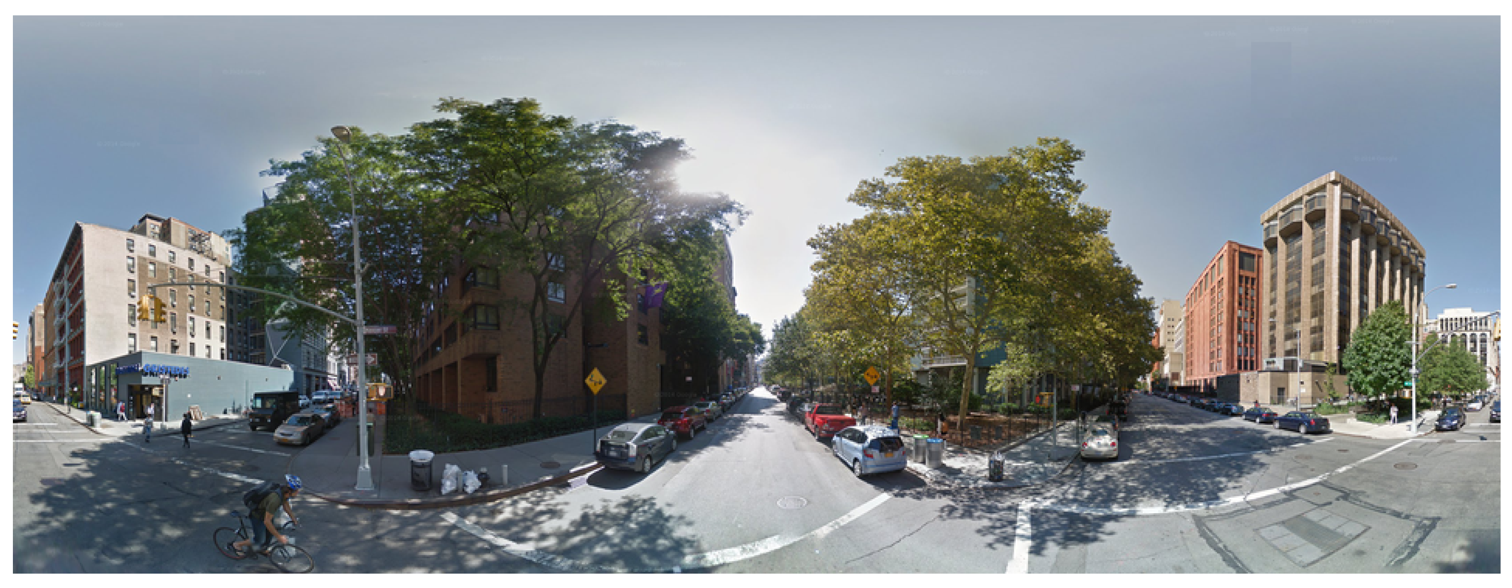
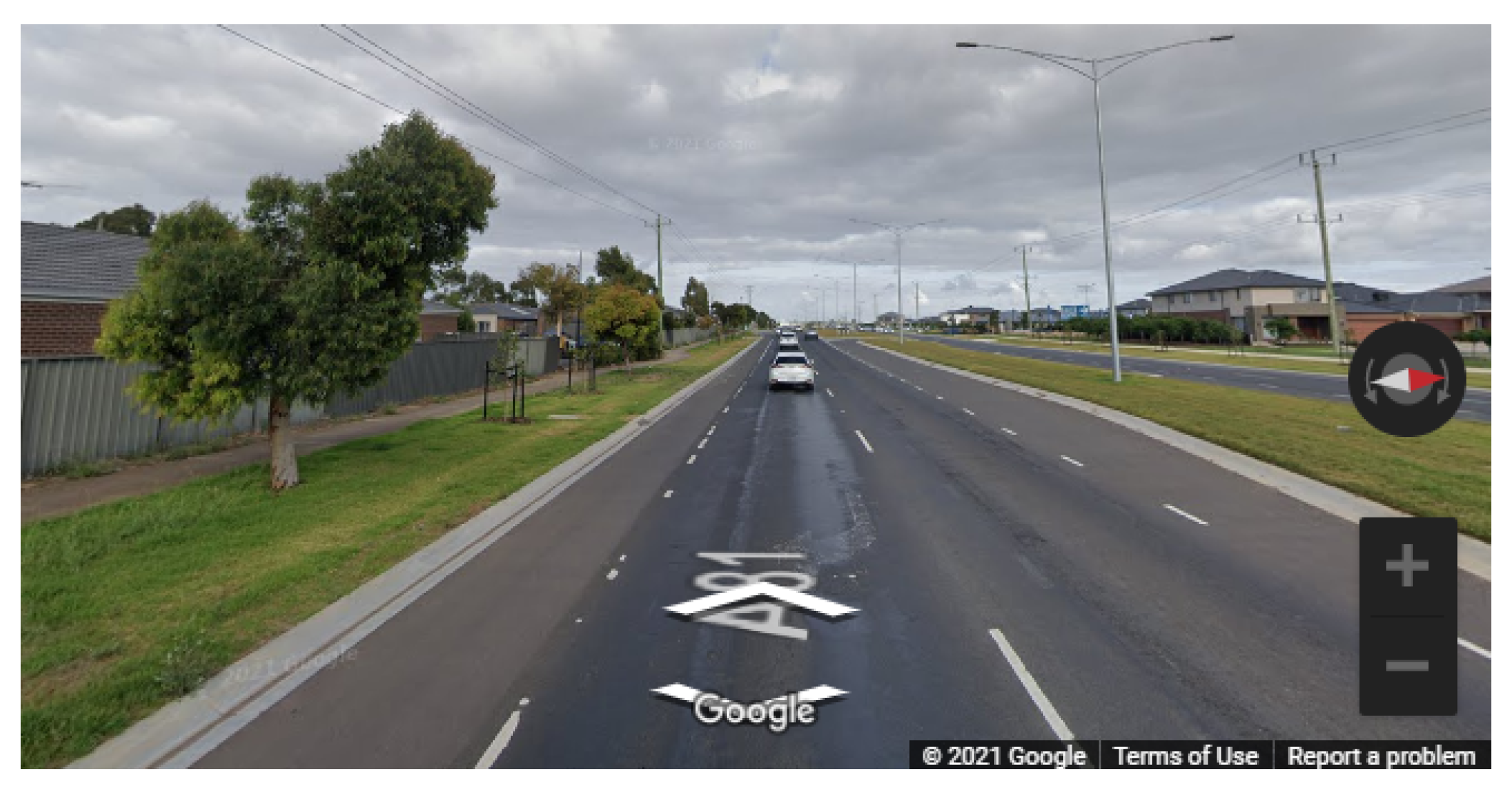
In this research work, Google street view images (GSV) [27] is used for the multiview semantic vegetation index (MSVI) estimation. A sample GSV image of a Wyndham Council in Melbourne, Victoria, is shown in Figure 3. The GSV panorama view is identical to the real-world view. The process of producing a 360 GSV panorama is to sequentially capture horizontal X-number (X = 6) images and vertical Y-numbers (Y = 3) images of the camera [28]. The GSV Image API (Google) [27], together with the position and travelling direction of the GSV car, can be used to obtain every accessible GSV image in an HTTP URL form, for example (https://maps.googleapis.com/maps/api/streetview?parameters (accessed on 15 August 2021). The static GSV image, as shown in Figure 4, can be retrieved for every point where the GSV is available by establishing URL parameters supplied via a specific HTTP request utilising the GSV Image API (Google) [27].
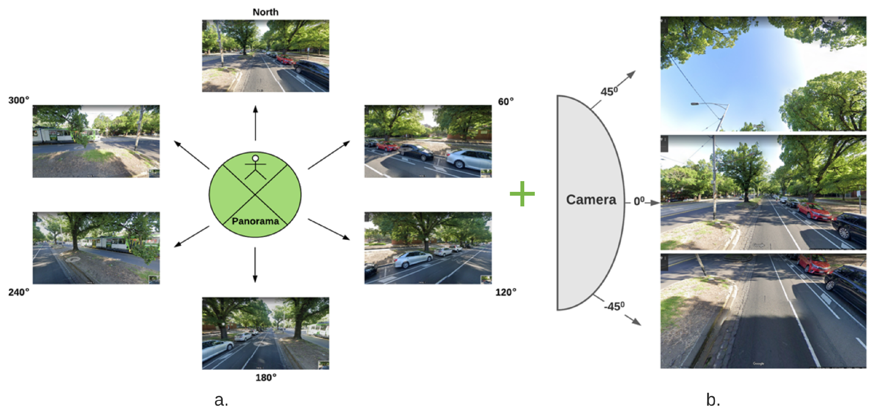
The GSV images for each sample site in six directions were collected as illustrated in Figure 5a, and in three vertical angles to determine the green areas visible to pedestrians as presented in Figure 5b. Therefore, 0, 60, 120, 180, 240, and 300 were set as the heading parameters whereas 45, 0, and −45 as pitch parameters. As a result, a total of eighteen images are captured for a specific location, ensuring that no vegetation area is left out of the index calculation. A Python programming language script is executed on all the GSV images to read and download them from each example site by automatically parsing the GSV URL.
2.3. Deep Semantic Segmentation
The act of grouping sections of an image in such a way that each pixel in a group correlates to the object class represented by the group as a whole can be defined as semantic segmentation for images in this manner [29,30]. The object classes in the current work correspond to trees and green vegetation terrain. Images can be segmented by allocating each pixel of an input image to a label class object, which is referred to as semantic image labelling [31]. Image segmentation is also known as semantic image labelling. This method often combines image segmentation with object identification techniques to produce a final result. Various deep learning-based segmentation models, such as FCN [32], DeepLabv3+ [33], and Mask R-CNN [34], are being developed for use in a variety of applications and environments. For the purpose of semantic vegetation segmentation and to calculate the vegetation index from GSV imagery in this research work, FCN [22] and U-Net [35] semantic segmentation models are used. Their selection was based on their high precision and excellent performance in medical imaging area. The results of the experiments demonstrate that deep learning-based segmentation models are effective at segmenting vegetation images using semantic attributes.
2.3.1. Fully Convolutional Network (FCN)
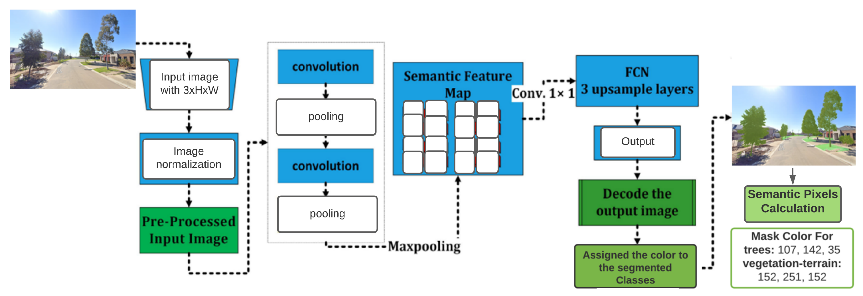
Fully Convolutional Network (FCN) [22] uses locally connected layers, such as up-sampling, pooling, and convolution, to achieve segmentation. The architecture does not include any dense layers in order to reduce the amount of time it takes to compute and the number of parameters it requires. A segmentation map uses two paths to obtain output: the first is a down-sampling road, which is used to collect semantic/contextual information, and the second is an up-sampling path, which is used to recover spatial features. The architecture of FCN is depicted in Figure 6. Fully convolutional network architecture (FCN) was presented by Long et al. [22] for robust segmentation by adopting fully convolutional layers in place of the last fully linked layers. This approach allows the network to generate a dense pixel-wise prediction as a result of the advancement. The combination of up-sampled outputs with high-resolution activation maps results in improved localisation performance, which is then passed to the convolution layers to produce the correct output. The performance of FCN motivated to employ it as an important component of the proposed approach.
2.3.2. U-Net
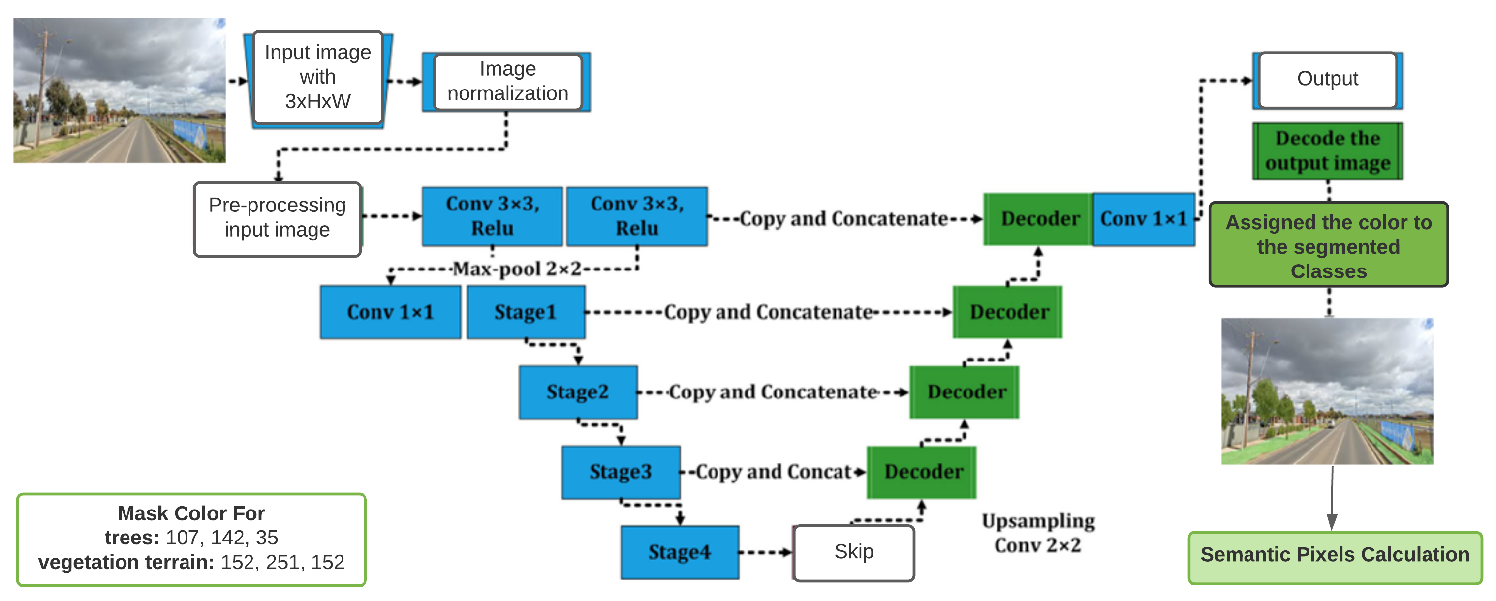
The second model employed in this work is U-Net [35], which has a similar encoder-decoder architecture to that of FCN but has two significant traits that distinguish it from the former. Since U-Net is symmetric, it bypasses the connections between the up-and down-sampling paths, which is useful when employed as a concatenation operator. Using the color variable, models assign a color to an item after they have been trained. The U-Net network (Figure 7) is built on an encoder-decoder architecture [35]. The encoder consists of a stack of convolutions and max-pooling layers that work together. The decoder is a symmetric expanding path that up-samples the feature maps with the use of learnable deconvolution filters, which can be learned. The major innovation brought about by this network is the way in which the so-called skip connections are utilised. To be more specific, they enable the concatenation of the output of the transposed convolution layers with the corresponding feature maps from the encoder stage during the convolution stage [36]. The main objective of this step is to get all the fine characteristics that were learned throughout the contracting stages in order to restore the spatial resolution of the original input image [35].
According to standard practice, in the U-Net approach, the input image is initially processed by an encoder path, which is comprised of convolutional and pooling layers that degrade the spatial resolution of the input image. It is then followed by a decoder path that restores the original spatial imagery resolution by adopting up-sampling layers followed by convolutional layers, which is a technique known as “up-convolution”. Apart from that, the network makes use of so-called skip connections, which connect the output of the relevant layers in the encoder path to the inputs of the decoder path by adding them to the inputs of the decoder path, whereas FCN allows pixel-wise classification performed for segmentation where features from initial convolutional layers are upsampled to develop deconvolution layers. These deconvolution layers develop the same size image, which is segmented on the basis of learnt features. Fine-tuning was performed to allow the network to learn efficient features of the vegetation region.
2.4. Vegetation Index Calculation from RGB Images
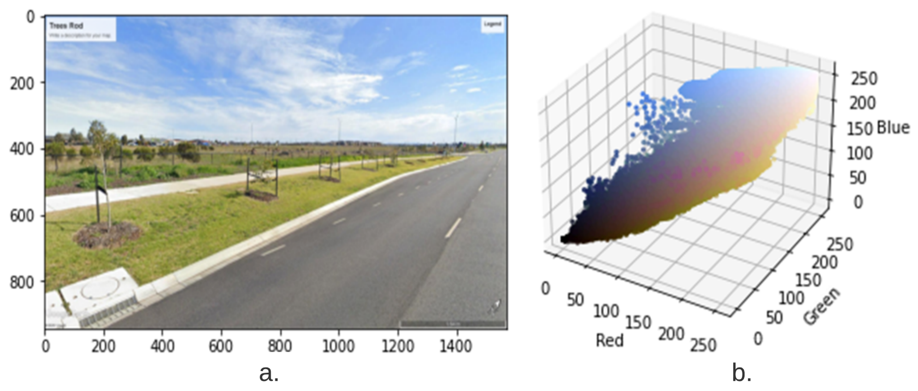
Various approaches are adopted in the literature for vegetation index calculation. Some of those are listed in Section 2.4.1. However, most of them used either color, threshold, or green area segmentation that might lead to promising results. To achieve robustness in vegetation index calculation, a semantic approach based on the unique color for each class of plants is proposed in this article. RGB color codes (107, 142, 35 and 152, 251, 152) for trees and vegetation terrain were assigned, respectively. After segmentation of the vegetation (trees and vegetation terrain), the respective masks are applied to calculate an accurate vegetation index as discussed in Section 2.4.2. For a better understanding of the RGB color space, the 3D data distribution in the RGB domain in Figure 8 is shown.
2.4.1. Green View Index (GVI)
Mohamed et al. [37] explored extracting green vegetation from remotely sensed multispectral images. It has been identified that both, i.e., near-infrared and red bands, are being utilised quite often for vegetation detection. One of the primary reasons is that on red bands, the vegetation shows less absorption, and on infrared, they show great reflection. However, GSV images cover only the blue, red, green, and near-infrared bands. It was established by Yang et al. [12] that the GVI value was affected by two factors: the size of a tree’s crown and the distance between the camera and the subject. A non-supervised classification methodology was used by Li et al. [13] to extract green vegetation from GSV images, which was justified by the fact that a significant number of GSV images were not available in the near-infrared band. According to their findings, green vegetation is significantly less reflective in red and blue bands. The red bands, on the other hand, are extremely reflective. As a result of this phenomenon, they developed extracting green vegetation from GSV images based on the natural hues of the images. There are a number of steps involved in the workflow.
- Step-1:
- First of all, the subtraction of red band from green band generates Diff 1, and subtraction of blue band from green band gives Diff 2.
- Step-2:
- Then the two images Diff 1 and Diff 2 were multiplied to create one Diff image. Normally, the green vegetation has greater reflectance values in the green band than the other two red and blue bands, and hence, the Diff image has positive green vegetation pixels.
- Step-3:
- The pixels that have lower values in the green band as compared to the red and blue bands exhibit negative values in the Diff image
- Step-4:
- As a result, an additional criterion was added stating that pixel values in the green band must be greater than those in the red band.
Usually, there were multiple spark points in the resulting images, after the initial classification images utilising the pixel-based classification approach were obtained as described in the steps above (Steps 1–4) [38]. The spectral vegetation variation has led to classifying individual pixels differently from their surrounding areas, leading to sparks in the classed image.
The above equation gives information regarding the available greenery in the image. Yang et al. [12] proposed the Green View Index (GVI), which measures the visibility of urban woods in terms of greenery. Its GVI was defined as the relationship between the total green space and four image(s) taken at the intersection of the road and the sum of the four images taken at the intersection as shown in the following equation:
where the presents the green pixels of the images taken in the direction of ith out of the four images taken in the (north, east, south, and west) directions. represents the total number of pixels in the image in the direction of ith. According to Li et al. [13], in this scenario, some surrounding vegetation may be missed from the calculation of the GVI since only four images cannot be seen in the fields of vision from the pedestrian view. Therefore, they modified the Equation (2) as below:
where denotes the number of green pixels in one of these images, which were taken in six directions with three vertical view angles for each sample site and were then averaged over all six directions. As a result, represents the total amount of pixels included within each one of the eighteen GSV images.
2.4.2. The Proposed Semantic Vegetation Index (SVI)
For robust calculation of the vegetation index of each sample location on the road or street, the approach of semantic pixels (SP) is used, which is based on the unique color pixels assigned to vegetation’s specific class (Vegetation terrain and trees) and are extracted based on the deep features through the use of a deep neural network. For index calculations, Google street view (GSV) images were used as such dataset is readily available. Therefore, in this investigation, a single image was used to calculate the vegetation index accurately based on the semantic pixels, so to cover all the vegetation area in the image. Hence, in each sample image, the number of semantic pixels will be determined as , with the area being the total semantic pixel numbers in one GSV image. The original Equation (1) has been updated and is now referred to as the semantic vegetation index (SVI).
where SVI stands for semantic vegetation index, n is the total number of images, denotes the amount of semantic pixel area representing greenery in an image, and denotes the total amount of pixels in an image.
Similarly, to calculate the multiview semantic vegetation index, a total of six images covering the 360° horizontal environment with three vertical angles of, i.e., 45, 0, and −45 are used. The process is shown in Figure 5b to calculate the vegetation index accurately based on the semantic pixels so that to cover all vegetation area. Hence, in each sample site, the number of semantic pixels will be determined as , with the Area being the total semantic pixel numbers in one of the 18 GSV images. Equation (3) has been modified to utilise semantic pixels for calculating the multiview semantic vegetation index (MSVI).
where MSVI stands for multiview semantic vegetation index, presents semantic pixels area of vegetation in input images which are taken from different pitch angles (45, 0 and −45) vertically as well as six horizontal direction covering 360 area, and represents the sum of pixels in an image from the eighteen images of GSV.
3. Results
3.1. Preparation and Annotation of Data Set
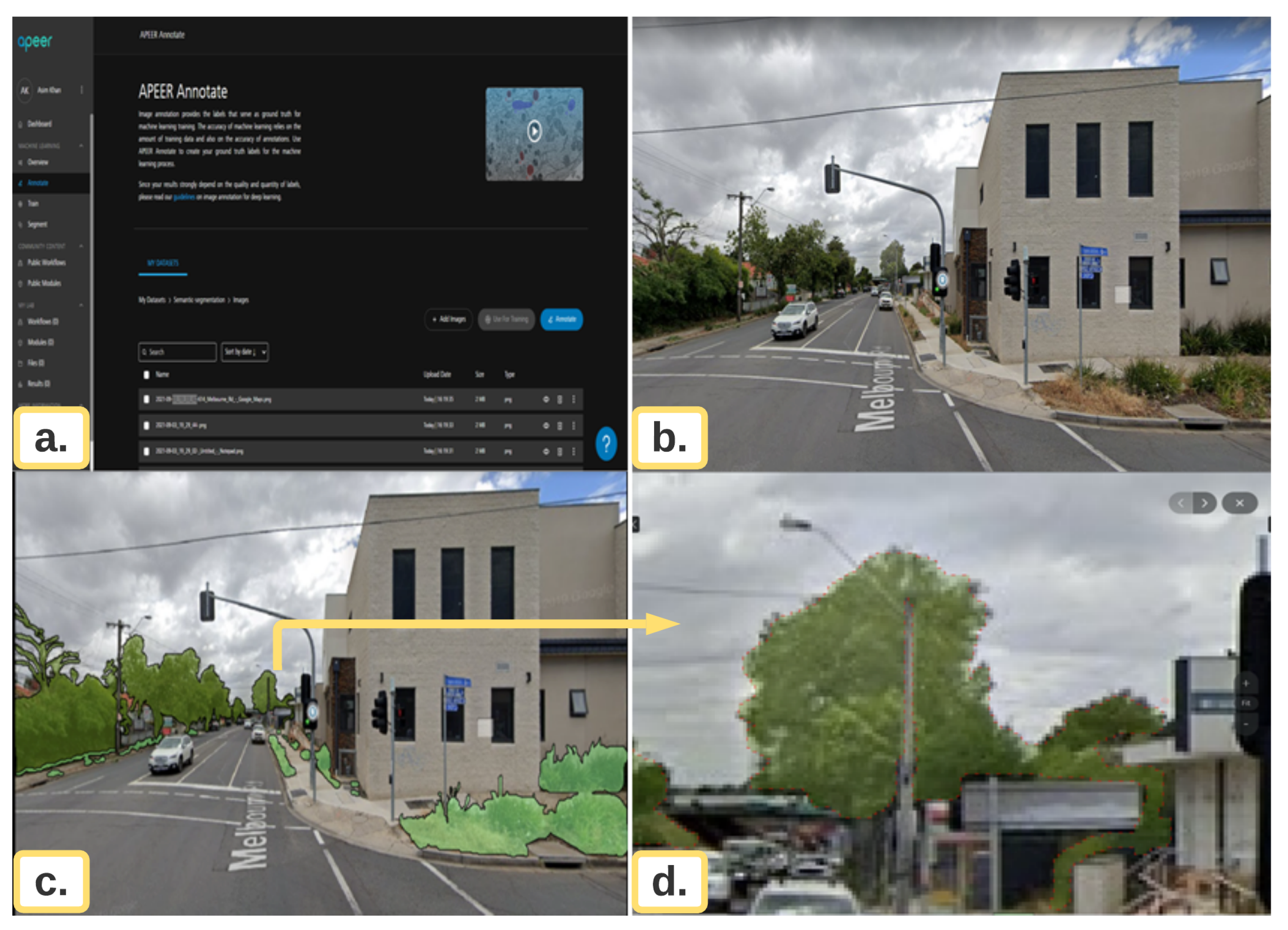
For the experiments and implementation of the proposed model, first, a total of 3000 Google street view (GSV) images were downloaded using a python script. The next step was the pre-processing of the dataset so that the images could be used for training and testing phases. For the annotation of the training data, a cloud-based tool known as “Apeer”, a ZEISS initiative [39], has been used. Image annotation generates labels that serve as the basis for machine learning training. Machine learning accuracy is determined by the amount of training data as well as the accuracy of annotations. The process of Annotation is summarised in Figure 9.
3.2. Experimental Environment Configuration
For the experiments and results, the hardware and software resources used are listed in Table 1.
3.3. Training of Deep Semantic Segmentation Models
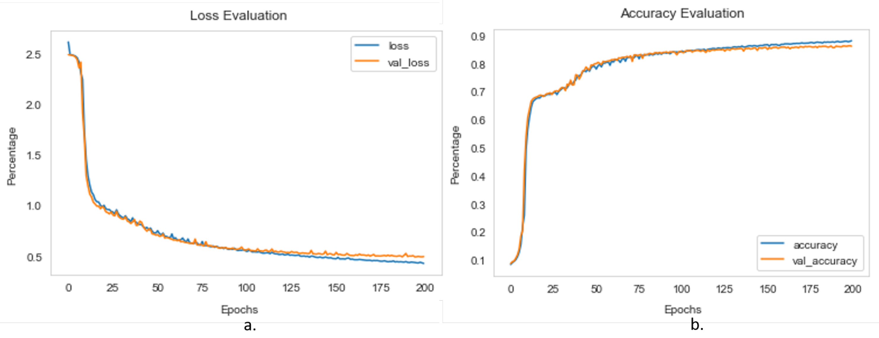
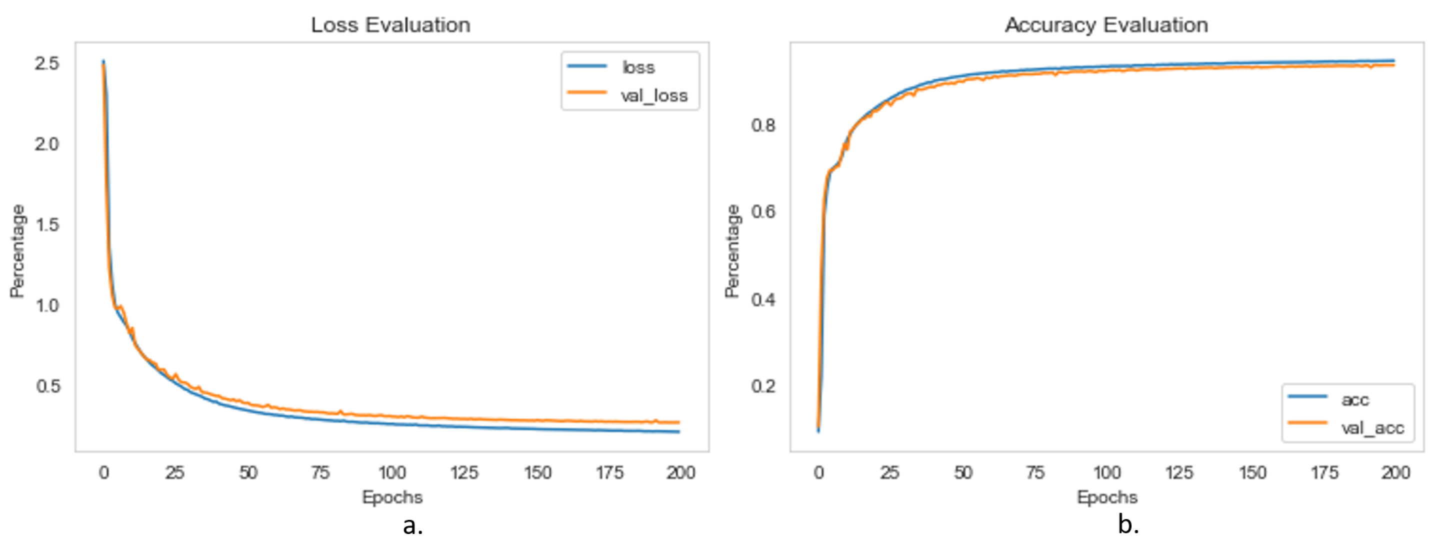
The complete data set was split up into three distinct sections: training, validation, and testing sets, each comprising 80%, 15%, and 5% of the total, respectively. Before starting the training, hyperparameters were set to avoid the overfitting and underfitting issues of the model. The hyper-parameters used for the training of semantic segmentation model were the following: batch size kept as 16, learning rate as 0.0001, loss function as categorical cross-entropy, number of iteration/epochs as 200, NMS threshold as 0.45, and an optimiser as stochastic gradient descent “SGD”. The training loss, validation loss, training accuracy and validation accuracy curve graphs are presented in Figure 10a,b and Figure 11a,b for the FCN Model and the U-Net Model, respectively. The accuracy curve for the U-Net beats the accuracy curve for the FCN, as shown in the graph in Figure 11.
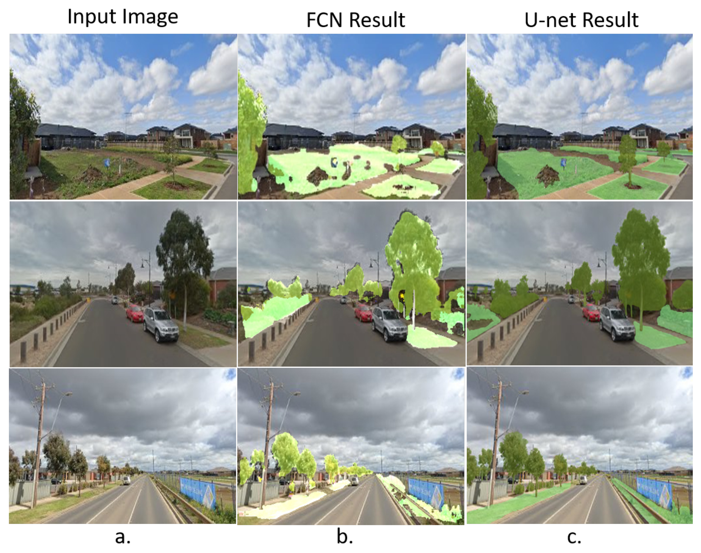
Some of the sample results using FCN and U-Net segmentation models are shown in Figure 12, and vegetation index values are computed using Equation (4). The vegetation index values calculated from FCN for the test input images are 43%, 30% and 32%, while vegetation index values calculated from U-Net for the test input images are 41.4%, 33%, and 37%. The results show that the U-Net segmentation model gives comparatively more accurate and promising results than the FCN segmentation model. The ground truth results are computed manually to compare the results after masking manually and then calculating the pixel values of the vegetation, using Adobe Photoshop application software. The computed results are in percentage, as evident from Equation (4). Thus, on the basis of the ground truth data, U-Net vegetation index results are quite promising and are more close to the ground truth results.
3.4. Performance Evaluation of Semantic Segmentation Networks
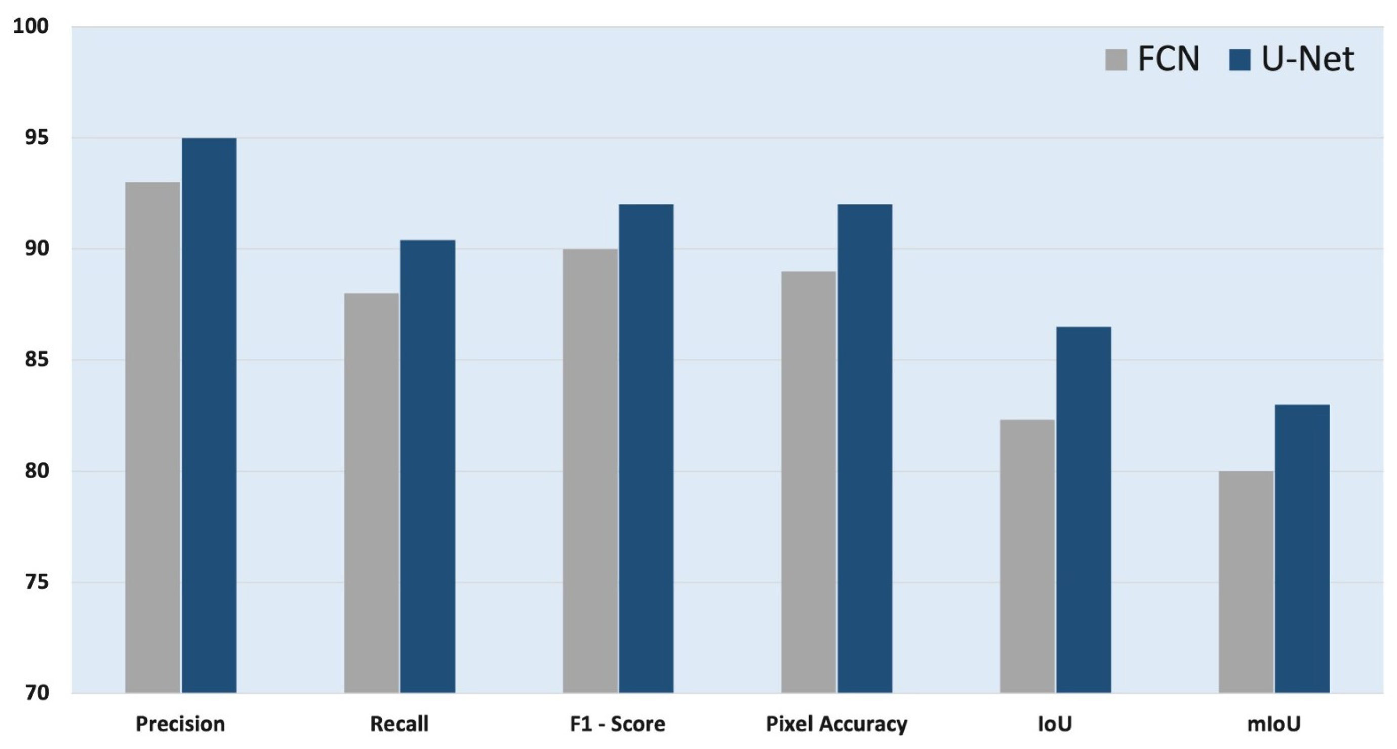
The performance of the semantic segmentation technique is evaluated using the metrics of precision, recall, F1-score, pixel accuracy (PA), intersection over union (IoU), and mean intersection over union (mIoU). Figure 13 shows the results of FCN and U-Net. The accuracy of object contour segmentation is measured using the PA method, while the accuracy of an object detector on a particular dataset is measured using the IoU metric. The mIoU is the average of IoU and is defined to show the overall enhancement of semantic segmentation accuracy.
3.4.1. Precision, Recall, and F1-Score
FCN and U-Net segmentation models were compared in terms of precision, recall, and F-measure. The results of the comparison are shown in Table 2.
Precision is defined as the relationship between the number of accurately segmented vegetation pixels and the total number of pixels segregated as a vegetation region by the technique. The recall is the ratio between the number of successfully segmented vegetation pixels and the total number of vegetation pixels in the labelled image.
The equation of F1-score is shown below,
3.4.2. Pixel Accuracy (PA)
In the evaluation of segmentation models, the pixel accuracy metric is the most commonly employed. It is defined as the accuracy of the pixel-wise prediction, given as
where k represents the total number of pixels in a test image, and is used to present the true positive predicted pixels as of class i, while presents the ground class i pixels as the number of pixels of class j.
3.4.3. Intersection over Union (IoU)
Intersection over Union (IoU) is also known as the Jaccard Index [40], and it is a typically used assessment statistic for segmentation models that is used to calculate their overall performance. As shown below, it is commonly defined as the ratio of intersection and union areas between the projected segmentation map and ground truth.
where k indicates the total number of classes, represents the number of true positives, and and represent the number of false positives and false negatives, respectively.
3.4.4. Mean-IoU (mIoU)
mIoU is yet another matrix that is commonly used in segmentation models. It is calculated as the average value of all IoU label classes taken as a whole. This type of report is commonly used to summarise the performance of segmentation models, given as
where k indicates the total number of classes, represents the number of true positives, and and represent the number of false positives and false negatives, respectively.
4. Comparative Analysis
The extraction of green vegetation from street view images is a difficult task because of a variety of factors, including the presence of shadows and spectral confusion between vegetation and other artificial green features (green walls, windows, shadows, signboards, etc.) Two studies are most relevant to this research: Yang et al. [12] used four GSV images in their work. As a result, Li et al. [13] modified the Green View Index (GVI) calculation, and they subsequently conducted a case study assessment of street vegetation using GSV images in the East Village of Manhattan District, New York City. They assert that the modified GVI may be a relatively objective measure of street-level greenery and that the use of GSV in conjunction with the modified GVI may be particularly effective in directing urban landscape planning and management practices.
For the purpose of comparison with the literature, sample images containing green vegetation, as well as green walls, signboards, and décor, were segmented and extracted for vegetation index calculation. Sample images segmentation results based on Li et al. [13] and Rencai et al. [15] are presented in Figure 14 and Table 3. From the results, it can be seen that the results of segmentation also included other green objects as vegetation because both the studies are principally based on green color. Both of the studies have mentioned this drawback in their studies and results, thus yielding an inaccurate vegetation index because of the inclusion of other green color objects. Hence, the vegetation index calculated values are higher as compared to our results. However, this study’s results included vegetation only while ignoring other green color objects for calculating the index because it is based on semantic segmentation, thus giving an accurate vegetation index value.
The multiview semantic vegetation index calculation for panoramic images taken at different angles horizontally (a) and with varying angles of pitch vertically (b), as shown in Figure 5, and the respective calculated vegetation index values are presented in Table 4. In the table, it is clear that the results of Li et al. [13] and Rencai et al. [15] are quite similar as both studies rely on the green color; hence, there are chances that during the calculation of the vegetation index, most of the time other objects of green color were included as mentioned before in the sample segmentation result shown in Table 3. Therefore, the results are inaccurate, and the vegetation index percentage indicated is larger than ours because both comparison studies employed the green area index, and the tram in the image was also used to compute green color in those studies shown in Figure 5. On the other hand, the proposed model extracted only vegetation index. The input image on the second row in the Figure 14 is taken from the paper by Li et al. [13] only for comparison purposes. There, they mentioned that their algorithm is based on the green color, thus including another green object during the calculation of the green view index.
5. Discussion
Based on the research study, the semantic segmentation leads to accurate index calculation. The publicly available GSV imagery of the urban areas was used to quantify street greenery, i.e., SVI of the urban streets. GSV are freely available to the public and can be used in machine learning/computer vision in an efficient way to perform multiple activities automatically. The SVI can be utilised as useful information/data for a better assessment of urban greenery by considering people’s envisioned vegetation on a street scale for urban planners and others. To assess the greenery of street vegetation, GSV images captured from the ground should be similar to those of pedestrians.
A single vertical point of view is insufficient to express correctly the surrounding vegetation index that pedestrians may observe; two vertical points of view are required. Therefore, the multiview semantic vegetation index (MSVI) is employed for six GSV images in this experiment to calculate the vegetation index, each spanning a 360° horizontal and three vertical angles of 45, 0 and −45, to calculate the vegetation index appropriately on the basis of the semantic pixels.
According to the findings of this study, GSV images are qualified for assessing street greenery, and the modified GVI may be a more objective measurement of street-level greenery. The multiview semantic vegetation index (MSVI) took advantage of the characteristics of GSV images, used 18 GSV images taken from different viewing angles, making the index more efficient for evaluating street greenery in urban areas. Because it measures the amount of visible urban greenery on the ground, the SVI formula is simpler to understand for the general public. As a result, it can give a monitoring tool to analyze gains or losses in urban vegetation. It may serve to help urban planners select the sites, sizes and varieties of greenery for best effect in the planning stage of an urban greening program. It, therefore, seems to be a promising instrument, not a mere gadget for users, for future urban planning and urban environmental management.
The strength of SVI lies in its robustness to color variations and viewpoint constraints. The limitation of the approach is its reliance on captured viewpoints and attributes of the captured image, like its zoom level and image quality. Therefore, if SVI is utilised for long-term vegetation monitoring, it is proposed that proper dataset normalisation and image registration scale or affine invariant [41] be used before SVI estimation.
6. Conclusions
This research paper proposes a robust vegetation index based on semantic segmentation called a multiview semantic vegetation index (MSVI). The Google Street View (GSV) imagery dataset is used for calculating and indexing the vegetation cover of an urban area of the Wyndham City Council in Melbourne, Australia. The MSVI is based on the deep features learned from a deep neural network to calculate the vegetation index of each sample location in the urban area. For vegetation segmentation, different deep learning-based semantic segmentation models, such as FCN and U-Net, were tried. Using the GSV data set, both segmentation models were trained and tested to improve their overall performance.
The proposed method for segmenting urban vegetation areas has yielded promising results. Generally speaking, U-Net shows better results than FCN. FCN and U-Net models achieve Precision of 93.2% and 95%, Recall of 87.3% and 90.8%, F1-score of 90.1% and 92.3%, pixel accuracy (PA) of 89.4% and 92.4%, IoU of 82.3% and 86.5%, and mIoU of 80% and 83%, respectively. The proposed MSVI index measures the broad visible urban greenery on the ground, which can assist urban planners and strategists in better understanding urban green spaces.
We intend to use this approach in the future for real-time vegetation index calculation using Google panoramic cameras such as Pilot Era 360°, Insta360 pro, and Insta360 pro2, which will be of great help in the quest for ecological improvement.
Author Contributions
Conceptualization, A.K.; methodology, A.K.; software, A.K.; validation, A.K. and W.A; formal analysis, A.K.; investigation, A.K.; resources, A.K.; data curation, A.K. and W.A.; writing—original draft preparation, A.K.; writing—review and editing, W.A., A.K, A.U. and R.W.R.; visualization, A.K. and W.A.; supervision, A.U. and R.W.R.; project administration, A.K., A.U. and R.W.R.; funding acquisition, A.U. and R.W.R. All authors have read and agreed to the published version of the manuscript.
Funding
This study received no external funding. However, Victoria University, Footscray 3011, Australia and Charles Sturt University, Port Macquarie (Campus), NSW 2444, Australia, equally funded.
Institutional Review Board Statement
Not applicable.
Informed Consent Statement
Not applicable.
Data Availability Statement
The data used to support the findings of this study are available subject to approval from the relevant departments through the corresponding author upon request.
Conflicts of Interest
The authors declare no conflict of interest.
References
- Song, X.P.; Hansen, M.C.; Stehman, S.V.; Potapov, P.V.; Tyukavina, A.; Vermote, E.F.; Townshend, J.R. Global land change from 1982 to 2016. Nature 2018, 560, 639–643. [Google Scholar] [CrossRef] [PubMed]
- Edgeworth, M.; Ellis, E.C.; Gibbard, P.; Neal, C.; Ellis, M. The chronostratigraphic method is unsuitable for determining the start of the Anthropocene. Prog. Phys. Geogr. 2019, 43, 334–344. [Google Scholar] [CrossRef] [Green Version]
- Rosan, T.M.; Aragão, L.E.; Oliveras, I.; Phillips, O.L.; Malhi, Y.; Gloor, E.; Wagner, F.H. Extensive 21st-Century Woody Encroachment in South America’s Savanna. Geophys. Res. Lett. 2019, 46, 6594–6603. [Google Scholar] [CrossRef] [Green Version]
- Wolf, K.L. Business district streetscapes, trees, and consumer response. J. For. 2005, 103, 396–400. [Google Scholar]
- Appleyard, D. Urban trees, urban forests: What do they mean. In Proceedings of the National Urban Forestry Conference, Washington, DC, USA, 13–16 November 1979; pp. 138–155. [Google Scholar]
- Nowak, D.J.; Hoehn, R.; Crane, D.E. Oxygen production by urban trees in the United States. Arboric. Urban For. 2007, 33, 220–226. [Google Scholar]
- Chen, X.L.; Zhao, H.M.; Li, P.X.; Yin, Z.Y. Remote sensing image-based analysis of the relationship between urban heat island and land use/cover changes. Remote Sens. Environ. 2006, 104, 133–146. [Google Scholar] [CrossRef]
- Onishi, A.; Cao, X.; Ito, T.; Shi, F.; Imura, H. Evaluating the potential for urban heat-island mitigation by greening parking lots. Urban For. Urban Green. 2010, 9, 323–332. [Google Scholar] [CrossRef]
- Camacho-Cervantes, M.; Schondube, J.E.; Castillo, A.; MacGregor-Fors, I. How do people perceive urban trees? Assessing likes and dislikes in relation to the trees of a city. Urban Ecosyst. 2014, 17, 761–773. [Google Scholar] [CrossRef]
- Balram, S.; Dragićević, S. Attitudes toward urban green spaces: Integrating questionnaire survey and collaborative GIS techniques to improve attitude measurements. Landsc. Urban Plan. 2005, 71, 147–162. [Google Scholar] [CrossRef]
- Gao, L.; Wang, X.; Johnson, B.A.; Tian, Q.; Wang, Y.; Verrelst, J.; Mu, X.; Gu, X. Remote sensing algorithms for estimation of fractional vegetation cover using pure vegetation index values: A review. ISPRS J. Photogramm. Remote Sens. 2020, 159, 364–377. [Google Scholar] [CrossRef]
- Yang, J.; Zhao, L.; Mcbride, J.; Gong, P. Can you see green? Assessing the visibility of urban forests in cities. Landsc. Urban Plan. 2009, 91, 97–104. [Google Scholar] [CrossRef]
- Li, X.; Zhang, C.; Li, W.; Ricard, R.; Meng, Q.; Zhang, W. Assessing street-level urban greenery using Google Street View and a modified green view index. Urban For. Urban Green. 2015, 14, 675–685. [Google Scholar] [CrossRef]
- Li, X.; Zhang, C.; Li, W.; Kuzovkina, Y.A. Environmental inequities in terms of different types of urban greenery in Hartford, Connecticut. Urban For. Urban Green. 2016, 18, 163–172. [Google Scholar] [CrossRef]
- Dong, R.; Zhang, Y.; Zhao, J. How green are the streets within the sixth ring road of Beijing? An analysis based on tencent street view pictures and the green view index. Int. J. Environ. Res. Public Health 2018, 15, 1367. [Google Scholar] [CrossRef] [PubMed] [Green Version]
- Zhang, Y.; Dong, R. Impacts of street-visible greenery on housing prices: Evidence from a hedonic price model and a massive street view image dataset in Beijing. ISPRS Int. J. Geo Inf. 2018, 7, 104. [Google Scholar] [CrossRef] [Green Version]
- Long, Y.; Liu, L. How green are the streets? An analysis for central areas of Chinese cities using Tencent Street View. PLoS ONE 2017, 12, e0171110. [Google Scholar] [CrossRef] [Green Version]
- Cheng, L.; Chu, S.; Zong, W.; Li, S.; Wu, J.; Li, M. Use of tencent street view imagery for visual perception of streets. ISPRS Int. J. Geo Inf. 2017, 6, 265. [Google Scholar] [CrossRef]
- Kendal, D.; Hauser, C.E.; Garrard, G.E.; Jellinek, S.; Giljohann, K.M.; Moore, J.L. Quantifying plant colour and colour difference as perceived by humans using digital images. PLoS ONE 2013, 8, e72296. [Google Scholar]
- Lopatin, J.; Dolos, K.; Kattenborn, T.; Fassnacht, F.E. How canopy shadow affects invasive plant species classification in high spatial resolution remote sensing. Remote Sens. Ecol. Conserv. 2019, 5, 302–317. [Google Scholar] [CrossRef]
- Schiefer, F.; Kattenborn, T.; Frick, A.; Frey, J.; Schall, P.; Koch, B.; Schmidtlein, S. Mapping forest tree species in high resolution UAV-based RGB-imagery by means of convolutional neural networks. ISPRS J. Photogramm. Remote Sens. 2020, 170, 205–215. [Google Scholar]
- Long, J.; Shelhamer, E.; Darrell, T. Fully convolutional networks for semantic segmentation. In Proceedings of the IEEE Conference on Computer Vision and Pattern Recognition, Boston, MA, USA, 7–12 June 2015; pp. 3431–3440. [Google Scholar]
- Dvornik, N.; Shmelkov, K.; Mairal, J.; Schmid, C. Blitznet: A real-time deep network for scene understanding. In Proceedings of the IEEE International Conference on Computer Vision, Venice, Italy, 22–29 October 2017; pp. 4154–4162. [Google Scholar]
- Li, Y.; Qi, H.; Dai, J.; Ji, X.; Wei, Y. Fully convolutional instance-aware semantic segmentation. In Proceedings of the IEEE Conference on Computer Vision and Pattern Recognition, Honolulu, HI, USA, 21–26 July 2017; pp. 2359–2367. [Google Scholar]
- Chen, L.C.; Yang, Y.; Wang, J.; Xu, W.; Yuille, A.L. Attention to scale: Scale-aware semantic image segmentation. In Proceedings of the IEEE Conference on Computer Vision and Pattern Recognition, Las Vegas, NV, USA, 27–30 June 2016; pp. 3640–3649. [Google Scholar]
- Council, W.C. Street Tree Planting | Wyndham City. 2021. Available online: https://www.wyndham.vic.gov.au/treeplanting (accessed on 15 August 2021).
- Street View Static API Overview | Google Developers. Available online: https://developers.google.com/maps/documentation/streetview/overview (accessed on 17 August 2021).
- Tsai, V.J.; Chang, C.T. Three-dimensional positioning from Google street view panoramas. IET Image Process. 2013, 7, 229–239. [Google Scholar] [CrossRef] [Green Version]
- Hao, S.; Zhou, Y.; Guo, Y. A brief survey on semantic segmentation with deep learning. Neurocomputing 2020, 406, 302–321. [Google Scholar] [CrossRef]
- Uhrig, J.; Cordts, M.; Franke, U.; Brox, T. Pixel-level encoding and depth layering for instance-level semantic labeling. In German Conference on Pattern Recognition; Springer: Berlin/Heidelberg, Germany, 2016; pp. 14–25. [Google Scholar]
- Guo, Y.; Liu, Y.; Georgiou, T.; Lew, M.S. A review of semantic segmentation using deep neural networks. Int. J. Multimed. Inf. Retr. 2018, 7, 87–93. [Google Scholar] [CrossRef] [Green Version]
- Liu, X.; Deng, Z.; Yang, Y. Recent progress in semantic image segmentation. Artif. Intell. Rev. 2019, 52, 1089–1106. [Google Scholar] [CrossRef] [Green Version]
- Chen, L.C.; Zhu, Y.; Papandreou, G.; Schroff, F.; Adam, H. Encoder-decoder with atrous separable convolution for semantic image segmentation. In Proceedings of the European Conference on Computer Vision (ECCV), Munich, Germany, 8–14 September 2018; pp. 801–818. [Google Scholar]
- He, K.; Gkioxari, G.; Dollár, P.; Girshick, R. Mask r-cnn. In Proceedings of the IEEE International Conference on Computer Vision, Venice, Italy, 22–29 October 2017; pp. 2961–2969. [Google Scholar]
- Ronneberger, O.; Fischer, P.; Brox, T. U-net: Convolutional networks for biomedical image segmentation. In Proceedings of the International Conference on Medical Image Computing and Computer-Assisted Intervention—MICCAI 2015; Lecture Notes in Computer Science; Springer: Cham, Switzerland, 2015; Volume 9351, pp. 234–241. [Google Scholar] [CrossRef]
- Garcia-Garcia, A.; Orts-Escolano, S.; Oprea, S.; Villena-Martinez, V.; Garcia-Rodriguez, J. A review on deep learning techniques applied to semantic segmentation. arXiv 2017, arXiv:1704.06857. [Google Scholar]
- Almeer, M.H. Vegetation extraction from free google earth images of deserts using a robust BPNN approach in HSV Space. Int. J. Adv. Res. Comput. Commun. Eng. 2012, 1, 134–140. [Google Scholar]
- Blaschke, T.; Lang, S.; Lorup, E.; Strobl, J.; Zeil, P. Object-oriented image processing in an integrated GIS/remote sensing environment and perspectives for environmental applications. Environ. Inf. Plan. Politics Public 2000, 2, 555–570. [Google Scholar]
- APEER. Available online: https://www.apeer.com/ (accessed on 15 August 2021).
- Hamers, L. Similarity measures in scientometric research: The Jaccard index versus Salton’s cosine formula. Inf. Process. Manag. 1989, 25, 315–318. [Google Scholar] [CrossRef]
- Khan, A.; Ulhaq, A.; Robinson, R.W. Multi-temporal registration of environmental imagery using affine invariant convolutional features. In Pacific-Rim Symposium on Image and Video Technology; Springer: Berlin/Heidelberg, Germany, 2019; pp. 269–280. [Google Scholar]
Figure 1.
A data flow diagram for the MSVI, which highlights the process of calculating the proposed vegetation index.
Figure 1.
A data flow diagram for the MSVI, which highlights the process of calculating the proposed vegetation index.

Figure 2.
The research area in Victoria, Australia, which was chosen for this study. (a) Victoria (Australia); (b) Wyndham City Council, Victoria, Australia; (c) one sample site and (d) a sample street view from a sample site.
Figure 2.
The research area in Victoria, Australia, which was chosen for this study. (a) Victoria (Australia); (b) Wyndham City Council, Victoria, Australia; (c) one sample site and (d) a sample street view from a sample site.

Figure 3.
A sample panorama image of a selected study site from Google street view imagery.

Figure 4.
A static image of a research site taken from Google Street View imagery.

Figure 5.
(a) Sample of images taken from pedestrian view in six different angles and (b) from pedestrian view, three images taken from three vertical angles (45, 0, −45).
Figure 5.
(a) Sample of images taken from pedestrian view in six different angles and (b) from pedestrian view, three images taken from three vertical angles (45, 0, −45).

Figure 6.
The architecture of fully convolution network (FCN) showing network processes. The masks for trees and vegetation are shown as RGB color codes.
Figure 6.
The architecture of fully convolution network (FCN) showing network processes. The masks for trees and vegetation are shown as RGB color codes.

Figure 7.
The architecture of U-Net showing network processes. The masks for trees and vegetation terrain are shown as RGB color codes.
Figure 7.
The architecture of U-Net showing network processes. The masks for trees and vegetation terrain are shown as RGB color codes.

Figure 8.
A sample image is presented in 3D color spaces for better understanding of data distribution: (a) sample image and (b) data distribution in RGB color space. As data in different color channels is tightly correlated, it provides inherent difficulties to differentiate color and semantic information in RGB domain.

Figure 9.
The process of data annotation shown in this figure: (a) a data annotation cloud based platform known as “Apeer”, (b) sample image for annotation, (c) after completion of annotation, and (d) area zoomed for annotation in (c) and pointed with arrow.
Figure 9.
The process of data annotation shown in this figure: (a) a data annotation cloud based platform known as “Apeer”, (b) sample image for annotation, (c) after completion of annotation, and (d) area zoomed for annotation in (c) and pointed with arrow.

Figure 10.
FCN segmentation model trend graphs for (a) training and validation loss and (b) training and validation accuracy.
Figure 10.
FCN segmentation model trend graphs for (a) training and validation loss and (b) training and validation accuracy.

Figure 11.
The U-Net segmentation model trend graphs for (a) training, validation loss and (b) training and validation accuracy.
Figure 11.
The U-Net segmentation model trend graphs for (a) training, validation loss and (b) training and validation accuracy.

Figure 12.
Segmentation and extraction of vegetation results from test input images: (a) input images, (b) results generated using FCN and (c) results generated using the U-Net model.
Figure 12.
Segmentation and extraction of vegetation results from test input images: (a) input images, (b) results generated using FCN and (c) results generated using the U-Net model.

Figure 13.
Performance evaluation of FCN and U-Net segmentation models.

Figure 14.
A sample of images and their segmentation (vegetation extraction) results using different approaches: (a) Sample input images, (b) Li et al. [13], and (c) Rencai et al. [15] and (d) SVI (proposed).


Table 1.
Configuration of experimental environment.
| Item Name | Parameter |
|---|---|
| Central processing unit (CPU) | Intel i7 9700k |
| Operating system | MS Windows 10 |
| Operating volatile memory | 32GB RAM |
| Graphic processing unit (GPU) | Nvidia Titan RTX |
| Development environment configuration | Python 3.8 + TensorFlow 2.5 + CUDA 11.2 + cuDNN V8.1.0 + Visual Studio 2019 |
Table 2.
Performance evaluation results.
| Segmentation Model | Precision | Recall | F1-Score | Pixel Accuracy | IoU | mIoU |
|---|---|---|---|---|---|---|
| FCN | 93.2 | 87.3 | 90.1 | 89.4 | 82.3 | 80 |
| U-Net | 95 | 90.8 | 92.3 | 92.4 | 86.5 | 83 |
Table 3.
Comparison table for vegetation segmentation and their vegetation index calculation using various vegetation extraction and index calculation approaches.
Publisher’s Note: MDPI stays neutral with regard to jurisdictional claims in published maps and institutional affiliations. |
© 2022 by the authors. Licensee MDPI, Basel, Switzerland. This article is an open access article distributed under the terms and conditions of the Creative Commons Attribution (CC BY) license (https://creativecommons.org/licenses/by/4.0/).
Share and Cite
MDPI and ACS Style
Khan, A.; Asim, W.; Ulhaq, A.; Robinson, R.W. A Multiview Semantic Vegetation Index for Robust Estimation of Urban Vegetation Cover. Remote Sens. 2022, 14, 228. https://0-doi-org.brum.beds.ac.uk/10.3390/rs14010228
AMA Style
Khan A, Asim W, Ulhaq A, Robinson RW. A Multiview Semantic Vegetation Index for Robust Estimation of Urban Vegetation Cover. Remote Sensing. 2022; 14(1):228. https://0-doi-org.brum.beds.ac.uk/10.3390/rs14010228
Chicago/Turabian StyleKhan, Asim, Warda Asim, Anwaar Ulhaq, and Randall W. Robinson. 2022. "A Multiview Semantic Vegetation Index for Robust Estimation of Urban Vegetation Cover" Remote Sensing 14, no. 1: 228. https://0-doi-org.brum.beds.ac.uk/10.3390/rs14010228
Note that from the first issue of 2016, this journal uses article numbers instead of page numbers. See further details here.