
Stream Boundary Detection of a Hyper-Arid, Polar Region Using a U-Net Architecture: Taylor Valley, Antarctica


National Center for Airborne Laser Mapping, The University of Houston, 5000 Gulf Freeway, Building 4, Room 216, Houston, TX 77204-5059, USA
*
Author to whom correspondence should be addressed.
Remote Sens. 2022, 14(1), 234; https://0-doi-org.brum.beds.ac.uk/10.3390/rs14010234
Submission received: 1 November 2021
/
Revised: 31 December 2021
/
Accepted: 1 January 2022
/
Published: 5 January 2022
(This article belongs to the Special Issue Remote Sensing of Dryland River Systems)
Abstract
:Convolutional neural networks (CNNs) are becoming an increasingly popular approach for classification mapping of large complex regions where manual data collection is too time consuming. Stream boundaries in hyper-arid polar regions such as the McMurdo Dry Valleys (MDVs) in Antarctica are difficult to locate because they have little hydraulic flow throughout the short summer months. This paper utilizes a U-Net CNN to map stream boundaries from lidar derived rasters in Taylor Valley located within the MDVs, covering ∼770 km2. The training dataset consists of 217 (300 × 300 m2) well-distributed tiles of manually classified stream boundaries with diverse geometries (straight, sinuous, meandering, and braided) throughout the valley. The U-Net CNN is trained on elevation, slope, lidar intensity returns, and flow accumulation rasters. These features were used for detection of stream boundaries by providing potential topographic cues such as inflection points at stream boundaries and reflective properties of streams such as linear patterns of wetted soil, water, or ice. Various combinations of these features were analyzed based on performance. The test set performance revealed that elevation and slope had the highest performance of the feature combinations. The test set performance analysis revealed that the CNN model trained with elevation independently received a precision, recall, and F1 score of , , and respectively, while slope received , , and , respectively. The performance of the test set revealed higher stream boundary prediction accuracies along the coast, while inland performance varied. Meandering streams had the highest stream boundary prediction performance on the test set compared to the other stream geometries tested here because meandering streams are further evolved and have more distinguishable breaks in slope, indicating stream boundaries. These methods provide a novel approach for mapping stream boundaries semi-automatically in complex regions such as hyper-arid environments over larger scales than is possible for current methods.
1. Introduction and Related Work
Stream width and stream cross sectional area are some of the most important metrics for hydrologic and sediment transport modeling and is a reflection of flow magnitude and sediment load capacity [1,2,3,4,5]. Global hydrological maps do not yet include complete hydrological datasets in the unglaciated regions of Antarctica such as the McMurdo Dry Valleys (MDVs) because their ephemeral nature makes streams difficult to detect. In the MDVs, channel runoff and sediment load capacity are a reflection of glacial ablation magnitudes, therefore it is important to extract stream extents to better understand spatial patterns of glacial ablation [6]. Patterns of channel dimension and occurrence across the MDV landscape will provide information on regional glacial runoff, hence ablation magnitudes. The MDVs were once considered stable, but due to an observed increase and leveling off of solar radiation, it is now making a shift to Arctic and alpine-style permafrost and glacial melt [7]. This has caused an increase in surficial warming on the glaciers and permafrost, leading to an increase in flood frequency and magnitude as well as the thawing of permafrost soils [7]. The thawing of permafrost decreases the consolidation of sediments, allowing for easier mobilization of sediments and landscape adjustments [8]. In order to obtain glacial runoff estimates and fluvial geomorphic changes across a large scale, the detection of stream boundaries and their extents are necessary. The detection of streams and their boundaries over other available temporal datasets in the MDVs will aid in the detection of fluvial geomorphic shifts spatially and supplement global hydrological datasets.
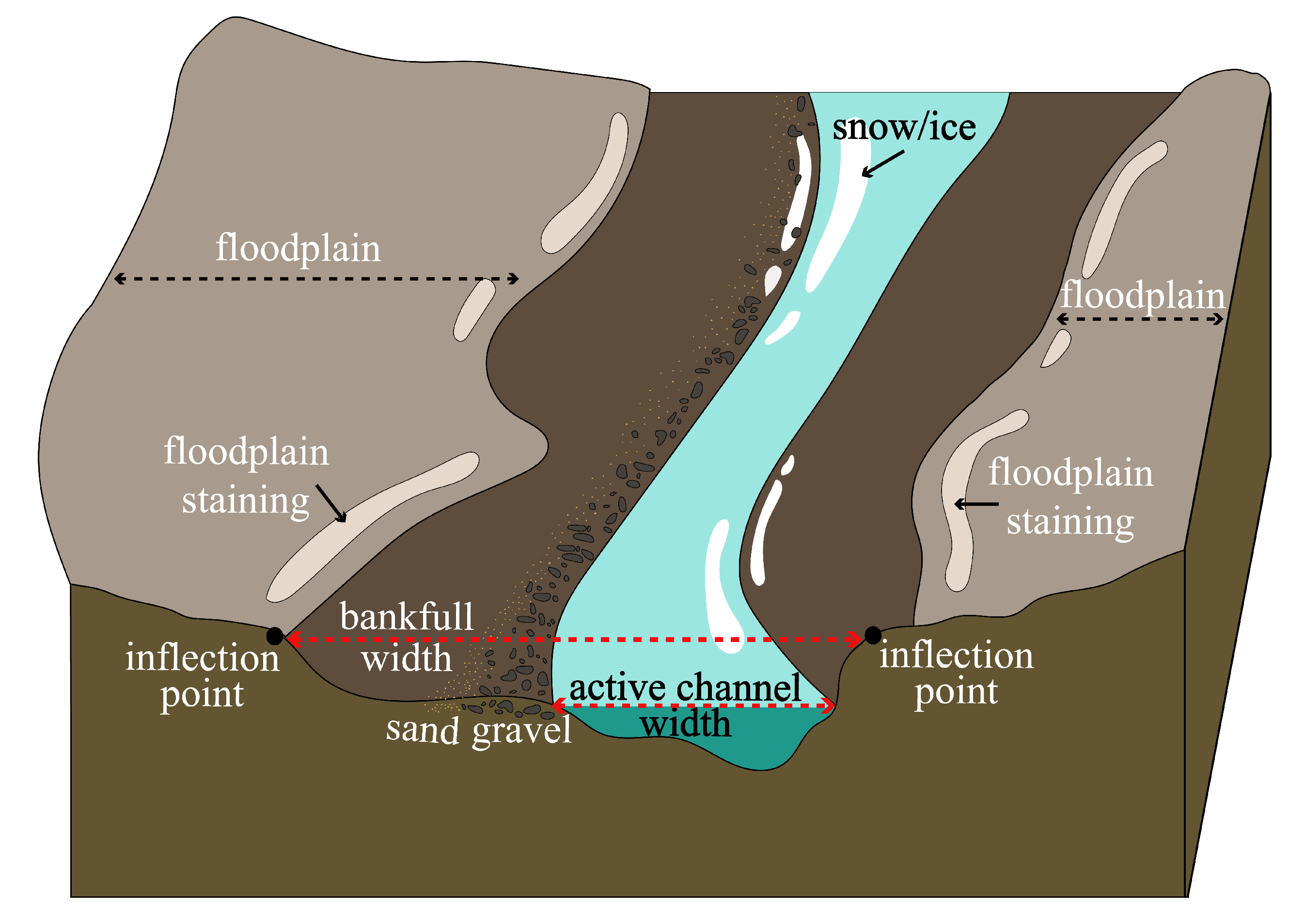
Detection of stream boundaries in hyper-arid regions is a difficult task, especially over large-scale regions because stream beds are periodically dry. Bankfull events typically recur every 1.5 to 2 years, but are even less frequent in arid climates than more humid regions [4,9]. Therefore, streams with very little activity may be narrow and not exhibit a clear distinction between active channel (normal high water lines) and bankfull extents (where the stream meets the floodplain), as a result we categorize these channel boundaries in the same class in this paper (Figure 1) [2,3]. Collecting sufficient stream boundary data in the field is arduous even over smaller, more hydrologically active areas, therefore remote sensing methods are required. Elevation and slope derived from lidar have been used for stream location and/or stream boundary detection in the past [1,3,10,11,12,13,14,15,16,17,18]. Digital elevation models (DEMs) have been commonly used to create flow accumulation models for both channel detection and centerline extraction for runoff simulation [10,11]. Stream boundaries have previously been estimated with topographic cues from lidar returns and/or imagery [3,12,17,18,19]. The stream centerline extraction and detection of the area of stream inundation and saturated soils of streams have also been accomplished using both elevation and intensity returns [14,15,16,20,21]. In this study, we consider an alternative stream boundary detection method using topographic and surface reflectance indicators as features from lidar-derived rasters for hyper-arid regions such as the MDVs. These topographic and surface reflectance features are utilized in a U-Net architecture for the detection of stream boundaries in the 770 km2 of glacier-free regions within Taylor Valley; one of the centrally located valleys the MDV. Based on a literature review, the use of deep learning for detection of small stream (∼10–150 m wide) extents in hyper-arid regions on a multi-basin scale has not been reported.
Existing remote sensing techniques are not suitable for large-scale, hyper-arid, polar regions such as the MDVs. MDV streams are ephemeral and runoff is controlled by local climatic changes that can vary spatially and on an hourly basis, therefore a stream may not be detected during data collection. Considering this, conventional methods that are reliant on waterbody extraction are not sufficient for our purposes. Existing remote sensing methods for channel extraction require a DEM and/or imagery where topographic cues are used to delineate channel extents [3,12,13,17].
Current stream boundary extraction methods utilize cross sections that are equally distanced and tangent to the stream centerline and/or require additional precipitation data or imagery [3,12,13,17,18]. In Li et al. [22] small rivers (>30 m wide) were extracted using spectral indices from Sentinel-2 imagery and DEM data. In hyper-arid regions such as the MDVs, even visual inspection of imagery may not be sufficient for manual detection of streams because stream flow, wetted soil, and ice change temporally and spatially. The main source of runoff in Taylor Valley is glacially sourced, and runoff magnitudes vary widely across the landscape, making stream boundary detection methods that rely on precipitation data unsuitable. Cross section-based methods must extrapolate the boundaries between cross sections, which can introduce large errors if the spacing between cross sections are too large. Accurately identifying stream boundaries for large regions with multiple complex watersheds is considered computationally expensive, as cross sections must be adequately proximal and wide enough across the channel length to accurately represent stream extents along the stream channel.
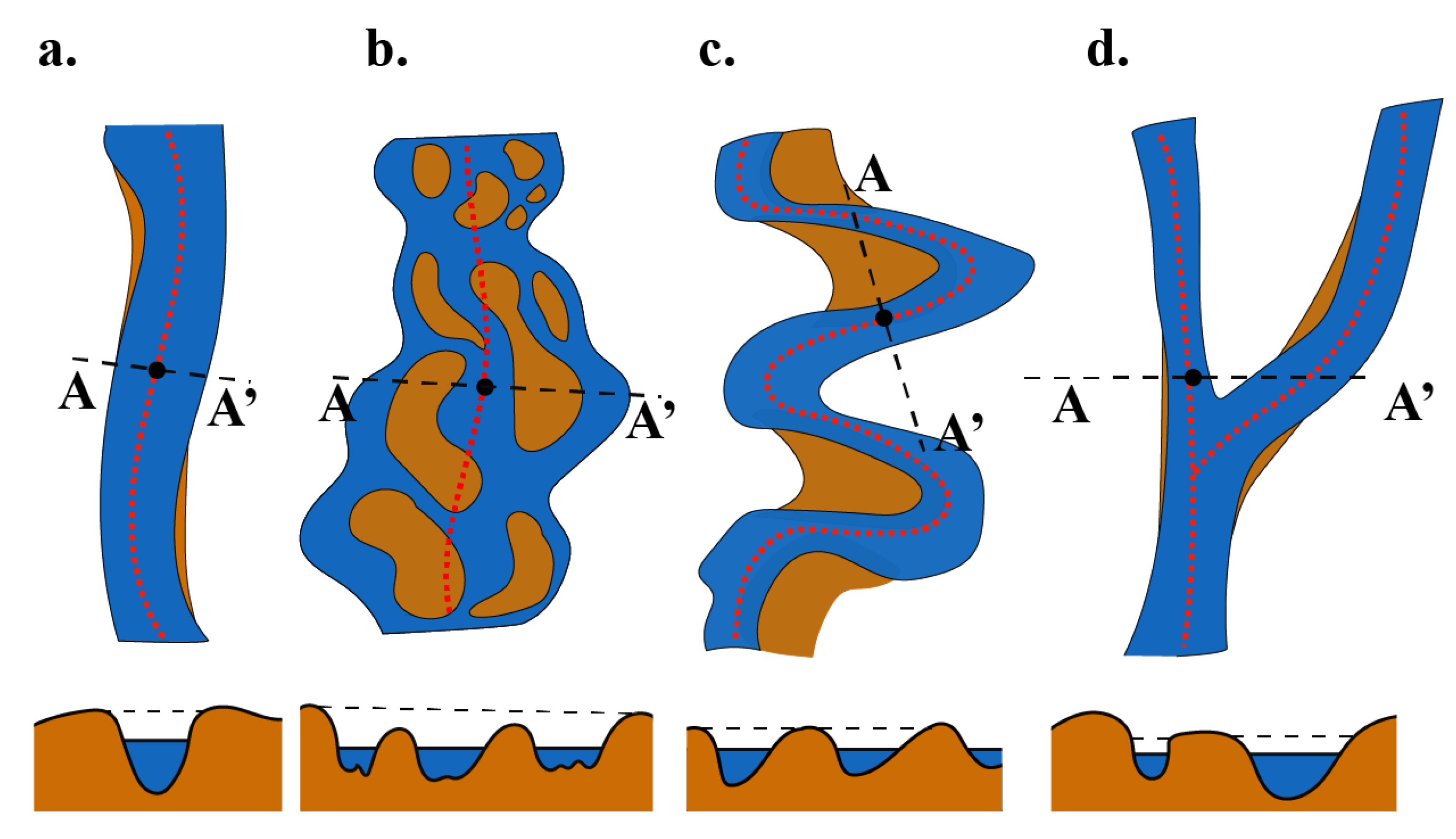
When cross section-based methods are used on large-scale regions with a wide range of stream geometries, they may require extensive editing. Cross section-based stream boundary detection methods typically are better suited for straight stream geometries compared to meandering and braided geometries. These algorithms may require manual editing of cross sections when it comes to streams that are meandering, multithreaded, at an intersection, or in close proximity to another stream (Figure 2b–d) [3,17]. Braided streams and streams that are close in proximity or near to a junction will exhibit multiple terraces and inflection points along the cross section, causing the algorithm to possibly misclassify stream boundaries by selecting the incorrect pair of inflection points (Figure 2b,d) [3]. Similarly, very tightly meandering streams at inner bends may have regions where the tangent to the stream centerline may cause a single cross section to intersect upstream and downstream rather than intersect the stream boundaries tangentially (Figure 2c) [3]. Instances such as these must be manually edited, which can become increasingly time consuming for extensive networks on a multi-basin scale [3]. Ideally, a stream boundary segmentation algorithm would be able to classify stream boundaries even along tightly meandering stream channels without manual editing of cross sections. Stream boundary extraction in Taylor Valley would require extensive manual editing with current methods as it has a wide range of stream geometries. In this study, we delineate stream boundaries across a wide array of stream geometries across the full extent of Taylor Valley using airborne lidar (ALS) collected in 2014. This study explores a stream boundary detection method that does not require cross sections, precipitation data, or imagery and can handle multiple basins with streams that are ephemeral in nature, such as Taylor Valley.
Convolutional neural networks (CNNs) have demonstrated excellent results in pattern recognition across scales in remote sensing [23,24,25]. A CNN is a type of neural network that can assign importance or weights and biases to different objects in an image in order to distinguish two or more classes [26]. Analogous to a human’s visual cortex, a CNN uses hidden layers to pass results successively to build a mathematical model for object identification [27]. CNNs have the ability to learn and detect objects at different localities and scales within an image, making it suitable for land surface segmentation [28,29,30]. Because of this ability, we use a CNN to detect dry stream networks and their stream boundaries in Taylor Valley, eliminating the need for cross sections; therefore set distanced interpolation. U-Net has been shown to be highly successful in pattern recognition and land surface segmentation using fewer training samples than other CNN algorithms [31,32]. Additionally, studies within remote sensing have shown that U-Net models create smoother and more connected features, which is important for hydrologic applications [21]. For these reasons, U-Net was selected for semi-automatic detection of streams and their stream boundaries in Taylor Valley.
The aim of this study is to define a semi-automatic method for stream boundary detection using high-resolution, lidar-derived rasters as features in a U-Net CNN architecture along stream channels in Taylor Valley. Our study only aims to detect stream boundaries that are visually distinguishable. Furthermore, this study does not try to discern stream boundary turning points from those caused by undercutting of the underlying strata. Provided that stream flow in the MDVs is unconventionally periodic and that there is limited field data, we are constrained to work with some level of ambiguity in the correct labeling of stream boundaries. Manual segmentation and prediction of stream boundaries is particularly difficult for less active, unmonitored streams. Given the extreme ephemeral nature of streams in the MDV, we propose a new method for detection of stream boundaries. Topographic, geometric, and lidar surface reflectivity indicators derived from airborne lidar were utilized for model training and prediction. To our knowledge, a semi-automatic stream boundary detection method that has been adapted for hyper-arid regions like the MDVs has not been attempted before on a multi-basin scale. This will aid future studies that would like to automatically classify stream boundaries in hydrologically similar regions for simulation of fluvial processes and estimation of geomorphic rates of change. In Taylor Valley specifically, detection of stream boundaries on available, temporally-spaced DEMs will allow researchers to detect and simulate changes within the different climatic zones to observe correlation between stream channel morphology and climatic perturbations.
2. Study Area
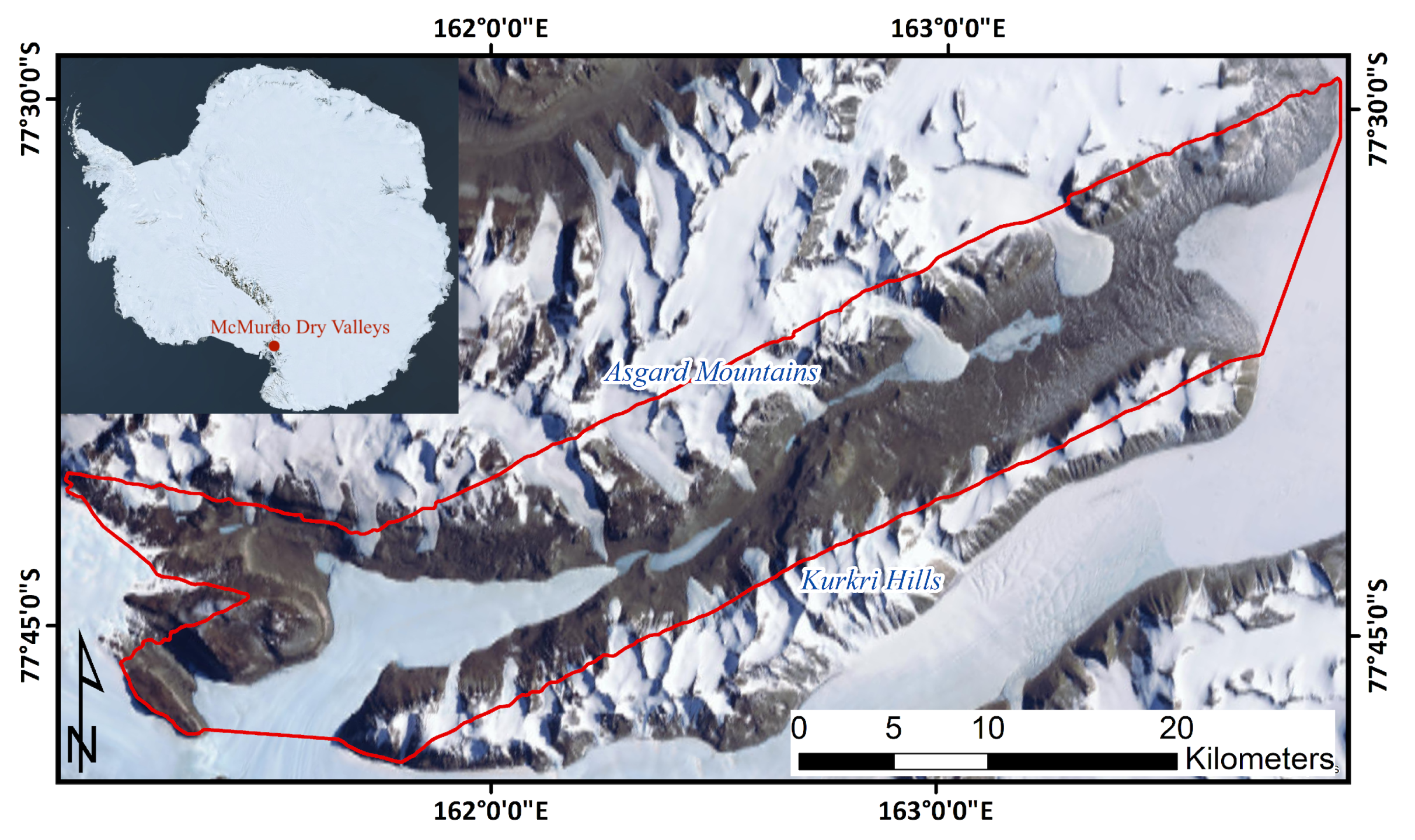
The study area is located in Taylor Valley in the MDVs in East Antarctica (Figure 3). Taylor Valley is centrally located in the MDVs and encapsulated by the Asgard Mountains, the Kurkri Hills, and the Ross Sea. Taylor Valley has one terminal glacier (Taylor Glacier) that flows from the Polar Plateau and 15 smaller alpine glaciers that flow from the side valleys. The Transantarctic Mountains to the west obstruct ice flow from the East Antarctic Ice Sheet to the valley producing a severe rain shadow. The valley is approximately 70 km long and 12 km wide. Elevation ranges from 0 to 2000 m and slopes are generally gentle to moderate in regions where stream flow exists. The valley primarily consists of glacial tills and fluviolacustrine deposits and at higher elevations there is exposed bedrock. The grounds are underlain by permafrost with active layers that are 45–70 cm thick near the coastal regions, 20–45 cm thick 60 km inland, and <20 cm along the polar plateau during the summer months [33].
The MDVs are one of the most arid regions of the world with sublimation (∼35 cm/year) exceeding what little precipitation (<10 cm/year) the valleys receive [34,35,36]. It is continuously dark during the winter months and temperatures can get as low as −60 C [37]. During the 6–12 weeks of summer, temperatures can reach 5 C [37]. Temperatures typically oscillate above and below the melting point of water throughout the summer days.
The MDVs have three geomorphic zones called microclimate zones. These zones are the upper stable zone (USZ), the inland mixing zone (IMZ), and the coastal thaw zone (CTZ) and are defined by summer temperature, soil moisture, and relative humidity. The sporadic runoff is almost entirely glacially sourced and flows to the perennially frozen closed-basin lakes [38,39]. The lack of vegetation allows streams with unconsolidated sediment to transport large sediment loads during times of flooding [38]. Due to the stream’s ephemeral nature, runoff may or may not exist at a given point in time. This makes the detection of the streams and its boundaries very difficult with existing methods. Several streams in Taylor Valley have already experienced extensive incision and bank undercutting due to climatic changes [6,7]. Although stream runoff is quite sporadic, runoff is predicted to become more frequent and will in turn further shape the valleys [40].
3. Methods
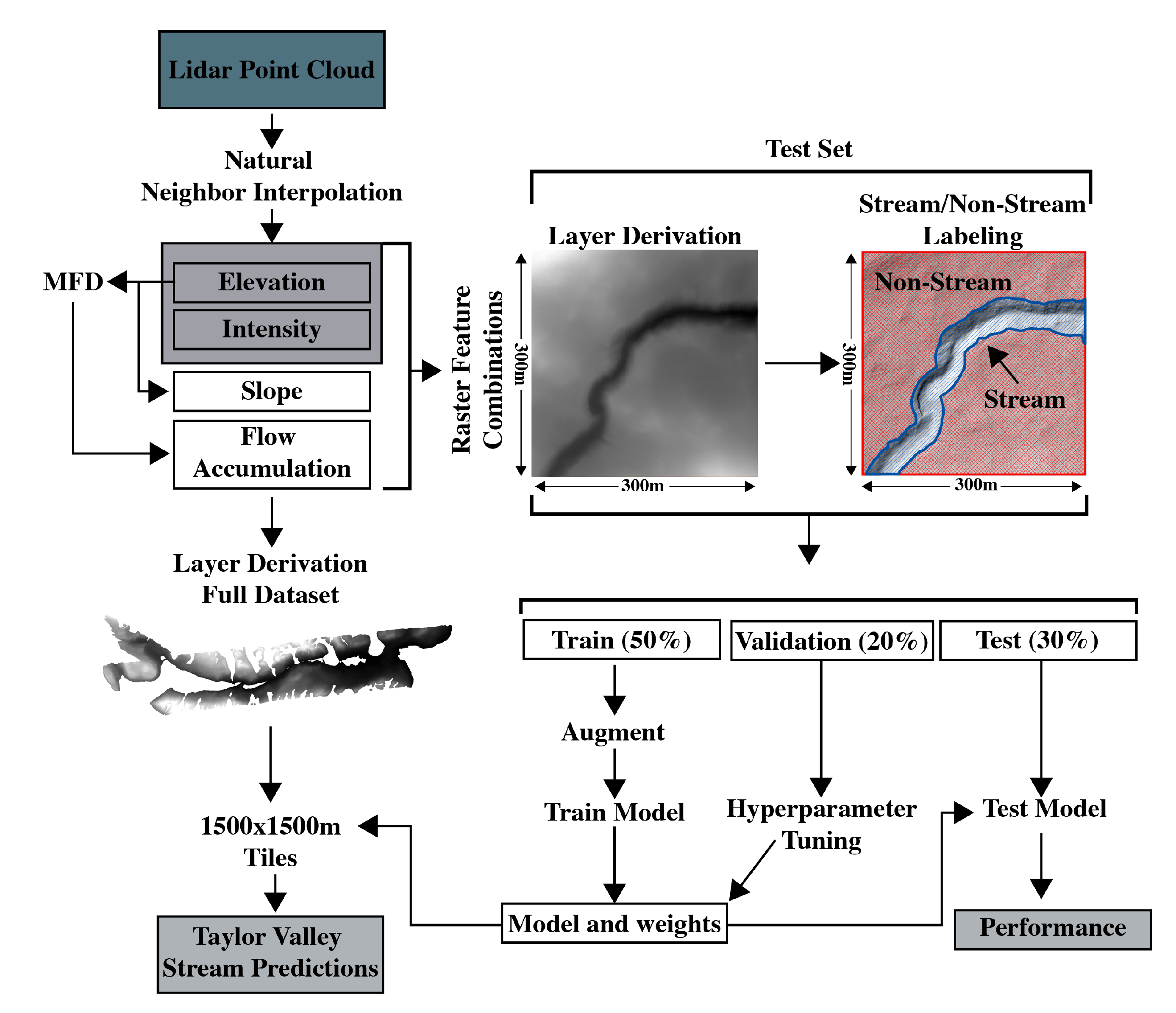
The creation of the training data, labeling, U-Net training, and prediction are depicted in Figure 4 and described in the subsections below.
3.1. Data Preparation
Airborne lidar data collected in 2014 by the National Center for Airborne Laser Mapping (NCALM) on the ice-free regions of Taylor Valley (∼560 km2) with a point density of 2.7 pts/m2 was utilized for stream boundary detection [41]. Digital imagery with 5–20 cm resolution collected simultaneous to the lidar survey as well as elevation and slope rasters were used for manual segmentation of stream boundaries to compile training data. The lidar surveys include the collection of ground point locations in space and raw intensity of lidar returns. Natural neighbor interpolation was used to convert the lidar dataset into a digital elevation model (DEM) and an intensity raster with spatial resolutions of 1 × 1 m2. A slope and flow accumulation model were calculated from the DEM using the slope and multi-flow direction (MFD) algorithms implemented in the ArcGIS software [42]. The DEM, intensity, slope, and flow accumulation rasters were then utilized as input features into the U-Net algorithm for training to find the best model for stream boundary prediction. Only the top performing models will be discussed here, but all performance metrics are available in Table A1.
The test set locations were manually selected, divided into raster tiles, normalized, and then manually digitized for ground truth. The selected feature rasters were broken up into 217 well-distributed 300 × 300 m raster tiles (covering ∼1% of the study area) throughout Taylor Valley. The test set includes regions with different channel geometries (straight, sinuous, meandering, and braided/intersecting streams) and stream sizes as well as those that lack streams with various topography. Stream test set locations were identified and selected based on evidence of stream existence where there was visibly distinguishable boundaries. Stream existence was determined using stream centerlines of major streams mapped by the Long-Term Ecological Research (LTER) and imagery exhibiting linear patterns of water, ice, or wetted ground downstream of glaciers and overlapped by stream centerlines extracted from MFD flow accumulation. Evidence of stream existence and imagery were used to avoid misclassifying turning points associated with other topographic features such as underlying strata.
The minimum and maximum within each tile for elevation, slope, intensity, and flow accumulation were calculated. To normalize the data the pixel values of each tile were subtracted from the tile minimum and then divided by the pixel value range. Normalization of slope and intensity by the minimum and maximum values help in regions where indicators are not as noticeable. This includes regions where stream boundaries exist, but are more easily detected with accentuation of the slope. Flow accumulation normalization was helpful for regions that had subtle patterns of ice or wetted ground. After normalization, the bit depth output was 8-bit unsigned. The resulting normalized elevation, slope, intensity, and flow accumulation, airborne digital imagery, and profiles were used for manually locating streams and digitizing their stream boundaries. Two classes were defined in the raster: “stream areas” and “non-stream areas”.
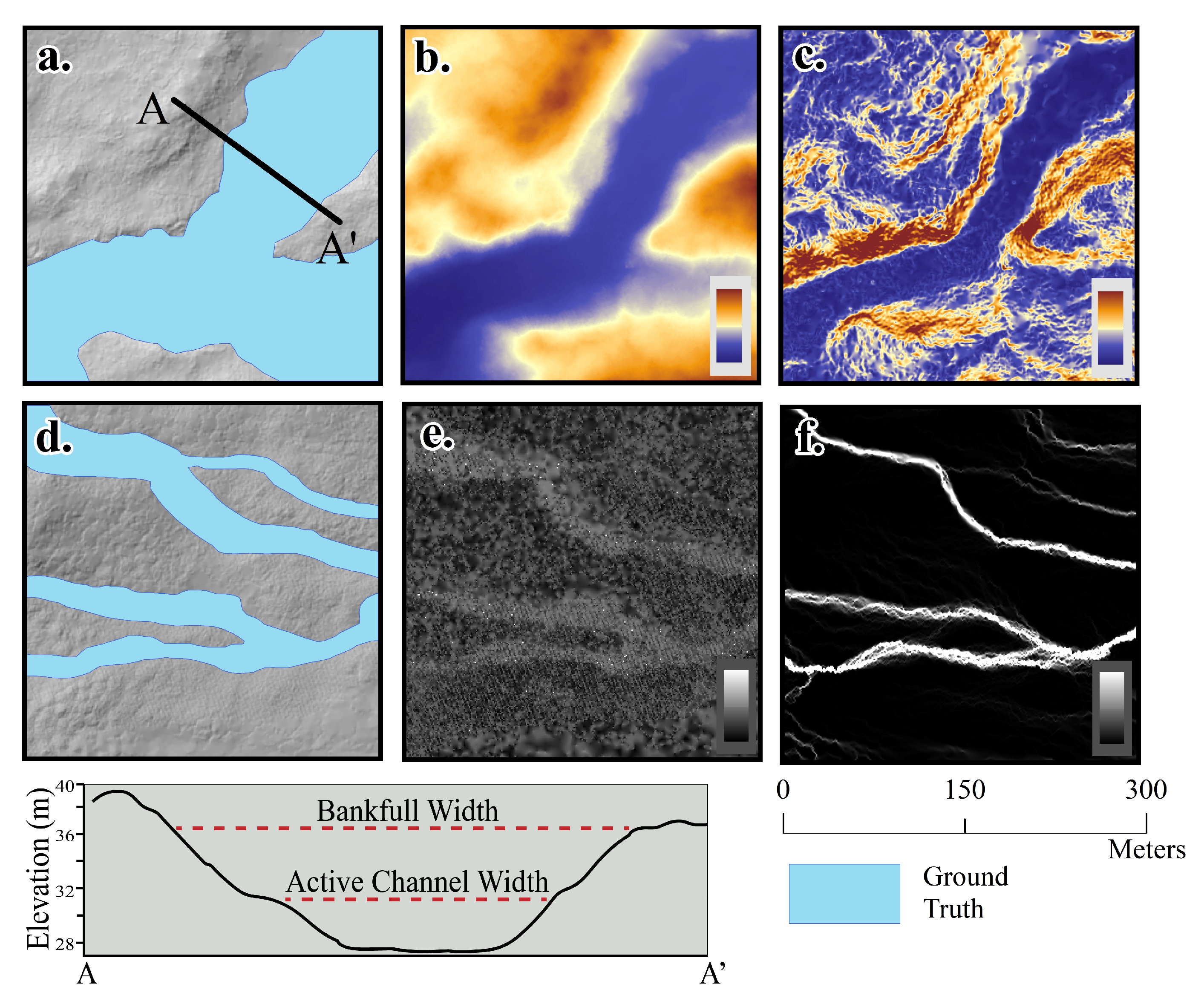
Stream boundary indicators include: inflection points, a change in sediment texture, and staining of the floodplain as diagrammed in Figure 1 [2]. Other stream indicators in the MDV are linear patterns of snow, ice, water, or wetted ground. Regions with concave profiles with topographic and visual indicators such as these were utilized to digitize stream boundaries. Topographic profiles, elevation, slope, and flow accumulation were used for manual detection of the stream boundaries using topographic cues such as inflection points and linear depressions (Figure 5a–c). The digital imagery, intensity, flow accumulation, and a hillshade were supplementary for manual stream identification (Figure 5d–f). Digital imagery, intensity, and flow accumulation can only provide visual information about stream location if either water, snow, or wetted soil exists in the channel, but cannot provide enough information for stream boundary detection.
It should be noted that CNN training relies on correctly labeled stream boundaries in the training data. Stream boundary segmentation is limited by the ability to manually differentiate stream boundary turning points from other topographic turning points such as underlying strata or outcrops. Any inflection points not distinguishable from stream boundaries such as underlying changes in strata in close proximity to stream boundaries can cause manual misclassification. Therefore, only samples with distinguishable stream boundaries such as breaks in slope were included. Prediction in turn will be focused on correctly identifying stream networks with distinguishable stream boundaries.
3.2. U-Net
U-Net is commonly used for raster segmentation. Normally, a RGB or greyscale image and its user classified ground truth are used as inputs; the output is an image where each pixel is assigned to a class [43]. This is accomplished by designing an architecture that incorporates a stacked convolutional layer and padding framework to ensure preservation of spatial resolution [44]. Furthermore, U-Net takes advantage of an encoder-decoder structure where the encoder learns abstract low-level features while the decoder develops high-level features through upsampling [45]. Essentially, the encoder decreases the spatial resolution of the image in order to increase computational efficiency and more easily differentiate different classes [46]. The decoder restores the image to it’s full-resolution to recover spatial information [46].
3.3. Training
The open source Landcover Dronedeploy tool was used for training and prediction of stream boundaries in Taylor Valley [47]. This code was implemented with fastai and PyTorch version 1.1.0 and uses a pre-trained ResNet-18 encoder model within the U-Net semantic segmentation framework. The various features and feature combinations with their corresponding ground truth were input into U-Net. A 50/20/30 split of the 217 samples was chosen for training, validation, and testing respectively and were used throughout the training. This split was chosen because the test set had to be large enough to decipher any trends in stream boundary segmentation accuracy (accuracy trends spatially and for stream geometry type), while not compromising the number of training data. The test set was manually selected to fairly represent the accuracies of each stream geometry and to get the right class balance. The training data was augmented with three 90 rotations. Prediction and fitting were carried out using the freely available Graphics Processing Units (GPUs) within Google Colaboratory (Nvidia K80s, T4s, P4s, and P100s) [48]. Depending on the available GPUs in Google Colaboratory, the total runtime for training and testing the algorithm was between four and six hours. The final tuned hyper-parameters included an epoch of 200, a batch size of 16, a learning rate of 1 × 10⁻⁵, and weight decay of 1 × 10⁻⁴. These parameters were found empirically based on the observed desirable loss curve characteristics and the speed of training, which include a smoothly decreasing loss as a function of epoch towards a low plateau. The top four performing models were saved for segmentation of the entire valley. A performance assessment of stream boundary segmentation was carried out on various combinations of the input features. Prediction performance was measured based on the proportion of correctly classified pixels. Performance metrics include recall, precision, and F1 score as they are commonly used metrics for evaluating a binary segmentation [49,50].
where: represents true positives, represents false positives, represents false negatives, P is the precision, R is the recall and is the F1 score.
The precision is representative of stream segmentation performance, while the recall represents the segmentation performance of non-stream regions. Performance was analyzed based on spatial location within Taylor Valley and by stream geometry (straight, sinuous, meandering, and those with braided or intersecting streams).
3.4. Prediction
Following model training, the full valley was broken up into 852 1500 × 1500 m2 overlapping tiles for prediction using the models with the four highest performing feature combinations: elevation, slope, intensity, and flow accumulation. Tiles were overlapped because pixels near the edges are susceptible to more error and may not include enough information to accurately predict stream boundaries. Tile sizes smaller than 1500 × 1500 m2 often classified the outer boundaries as “stream areas” and misclassified stream bottoms as “non-stream”. This resulted due to tiles only including a section of a stream and therefore did not provide enough information for the algorithm to accurately predict. Increasing the tile size from 300 × 300 m2 to 1500 × 1500 m2 provided a larger picture for the model so it could predict bankfull boundaries with very little noise across the full valley. Normalization across a larger area may cause a larger deviation in pixel values, which could cause misclassification of less active streams as ground because a larger tile will exhibit more gentle gradient changes with normalization compared to a smaller tile. The total runtime for prediction across the full valley after the model is trained was ∼15 min. A subset of the data was selected and digitized for a visual comparison of the predictions from the top two performing models.
4. Results
Here, we discuss the U-Net segmentation performance of stream boundaries on a valley-wide scale in Taylor Valley. Performance results from the different feature combinations are shown in Table 1. Training each of the models with single features outperformed the models that had two or more features. All four of these features were found to perform well on the test set with the precision, recall, and F1 score ranging from to , to , and to , respectively (Table 1). Elevation and slope had the highest performances in stream boundary prediction over the test set and had similar accuracy metrics.
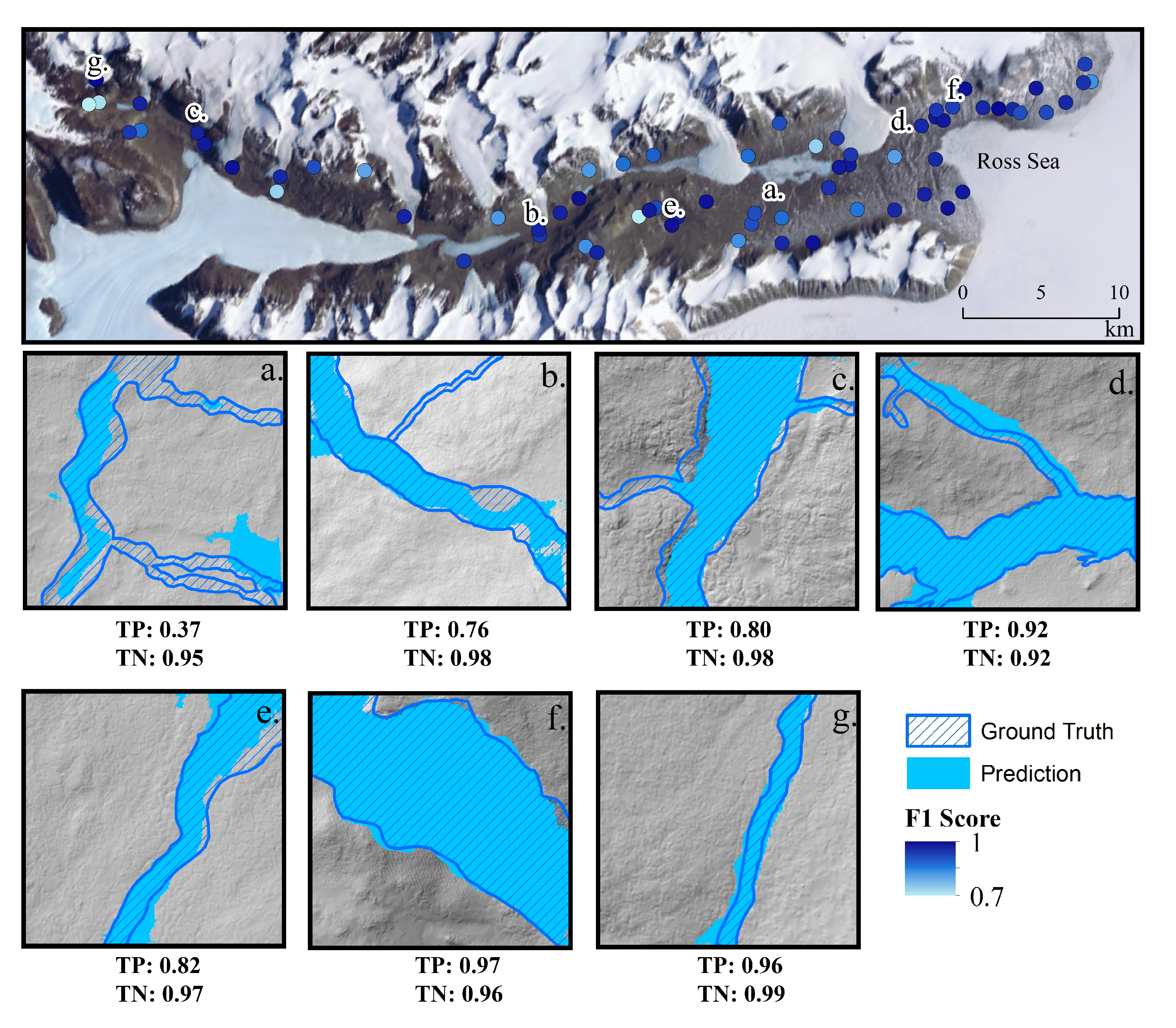
Spatial prediction accuracy on the test set was nearly identical for elevation and slope, therefore the elevation-based model is the only one depicted. The prediction of stream boundaries on the test set across Taylor Valley show that coastal regions typically have higher performance with F1 scores of 0.81–0.99 (Figure 6). Other regions across the valley had mixed F1 scores of 0.70–0.98, with a decreased score approaching slightly inland. The average for true positives was 0.71, while for true negatives it was 0.93. Figure 6a–f show the general trend in Taylor Valley where underprediction is more common than overprediction. Regions that did not perform as well did not have as distinct breaking points in slope at the stream boundaries.
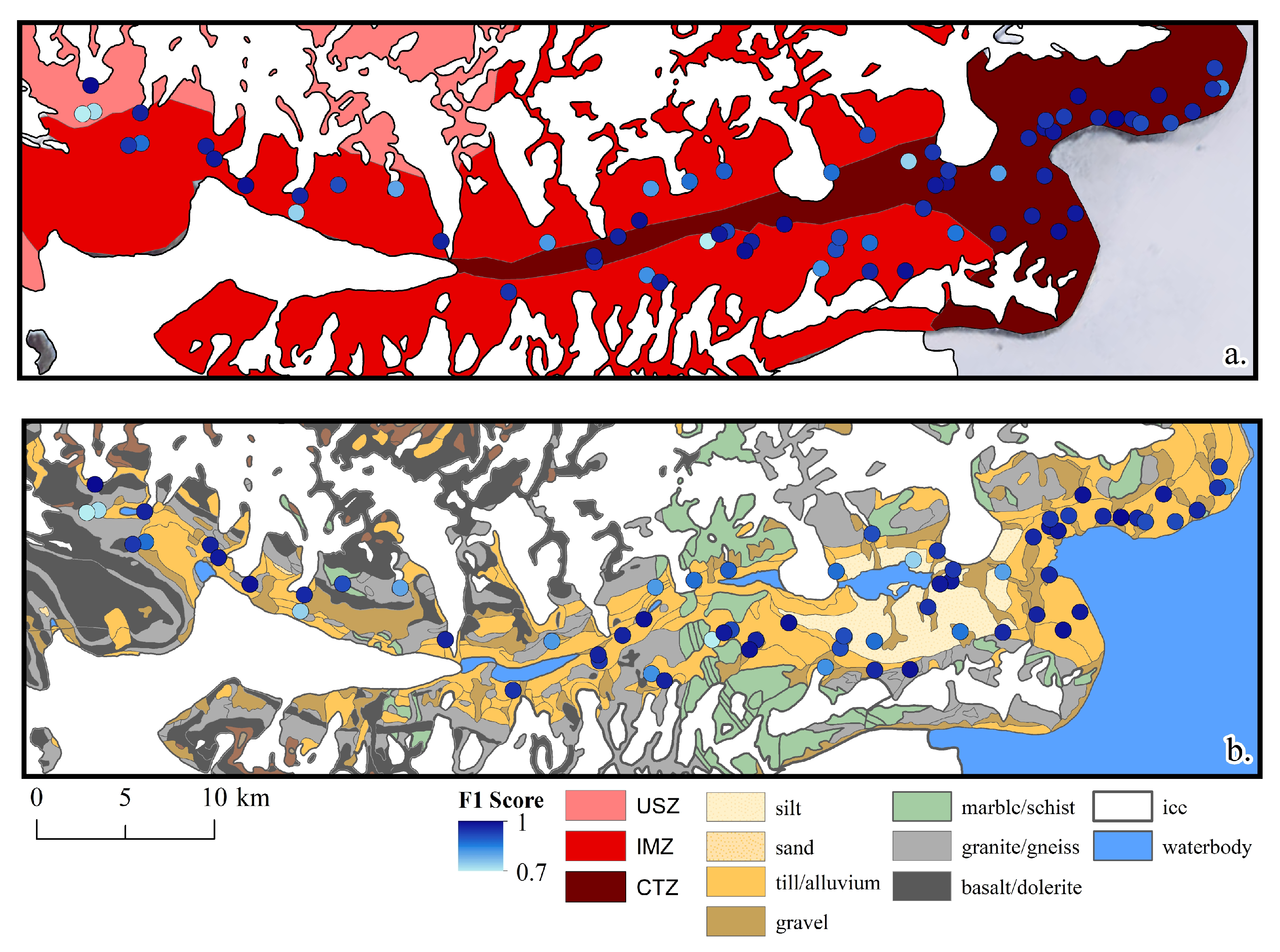
When prediction accuracy was compared to the three microclimate zones (CTZ, IMZ, and USZ), the CTZ acheived the most confident results (Figure 7). However, upon inspecting outcrop geology and stream boundary prediction accuracy, there seemed to be some correlation of high stream boundary prediction to outcrop geology. The glacial till region near the coast received the highest prediction accuracies on average. The test regions that had lower stream boundary prediction were typically located at or near bedrock (in grey and green) (Figure 7).
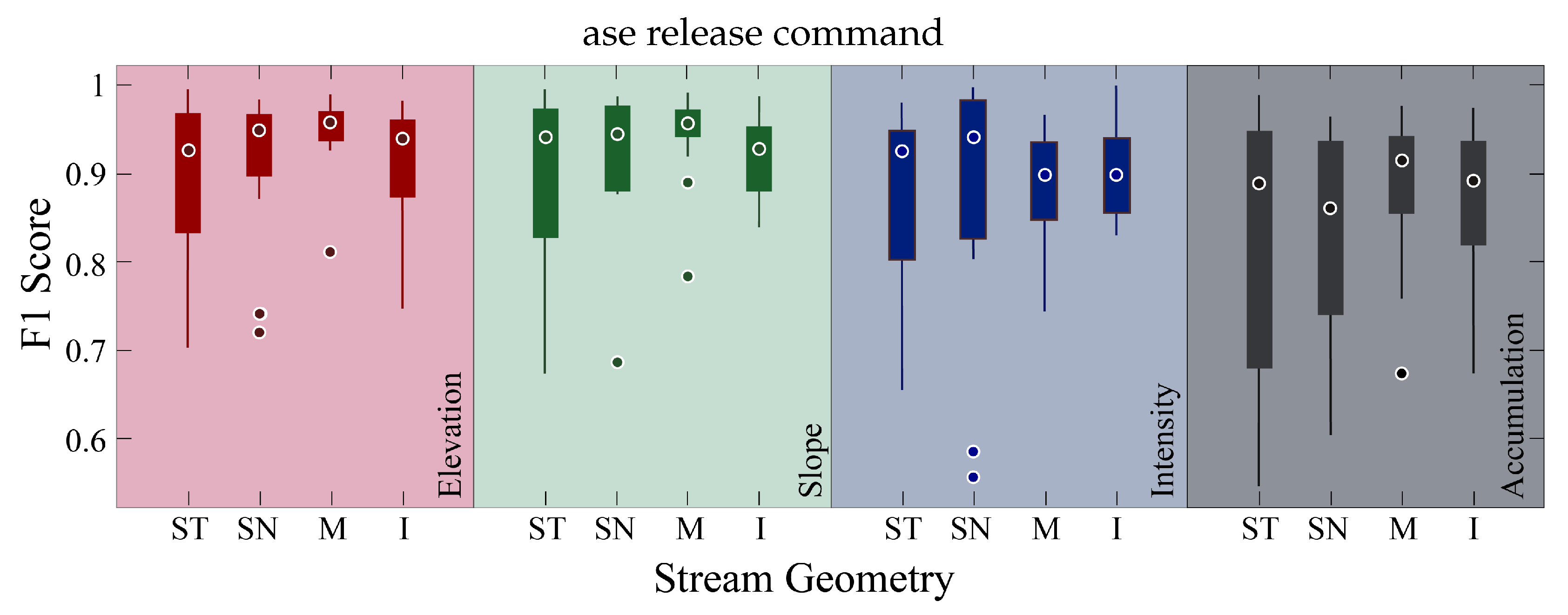
The performance of stream boundary prediction was assessed across the four feature classes and over different stream types (straight, sinuous, meandering, and braided or intersecting streams) (Figure 8). The elevation and slope features received the highest F1 scores and had a lower range of F1 scores across the different stream types (Figure 8). Straight streams across all of the features performed the worst while meandering streams typically performed the best followed by intersecting and sinuous streams (Figure 8). In contrast, cross section-based methods perform better on single-channel streams in comparison to braided or tightly meandering channels. The lidar return intensity and flow accumulation features received the lowest precision, recall, and F1 score, therefore they are not discussed here in length, rather elevation and slope will be our main focus.
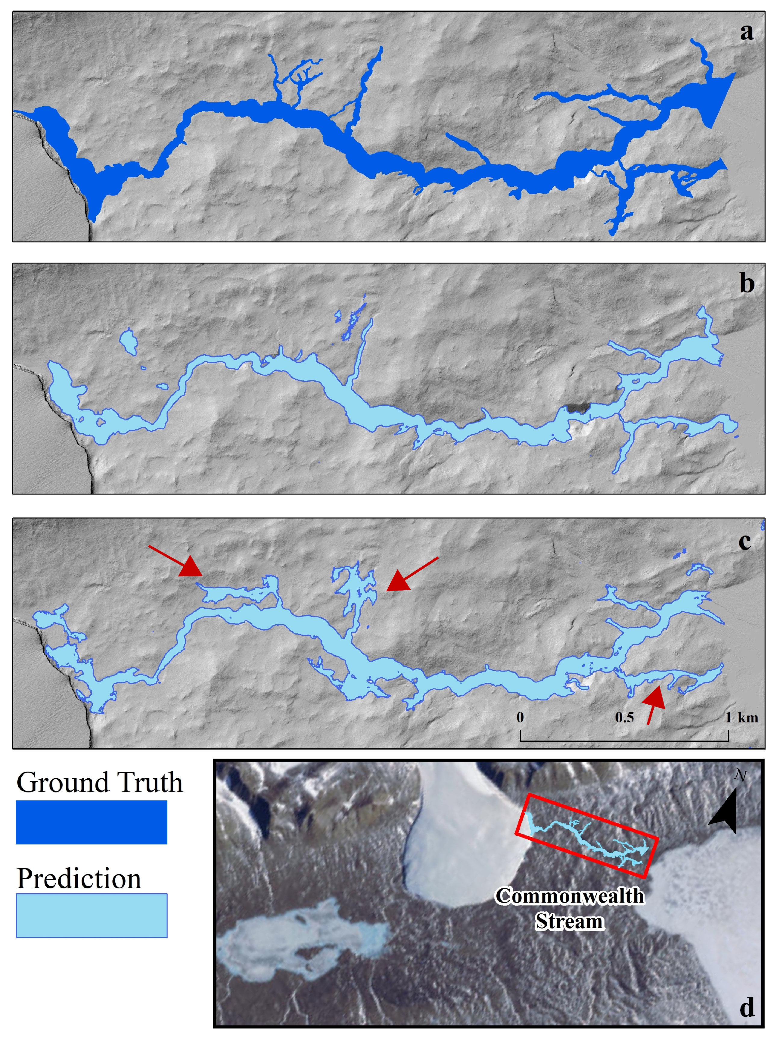
The manually labeled test images and the stream boundary prediction agree with each other (Figure 6). The prediction over Commonwealth Stream located between Commonwealth glacier and the Ross Sea show that elevation and slope are comparable to the manually digitized ground truth (Figure 9). Elevation was a little less noisy and did not over-predict the stream boundaries compared to slope (Figure 9). Tributaries were more difficult to detect accurately than the main branch (Figure 9).
5. Discussion
Overall, both the elevation and slope features had the highest performance for stream boundary segmentation. The intensity and flow accumulation features do not provide topographic information needed to accurately identify stream boundaries as indicated by features such as inflection points. These two features were meant to be supplementary support features to slope and elevation, however increasing the dimensionality of attributes with a very small test set increases the difficulty of convergence [51]. In more hydrologically active regions, models including intensity may have higher performance in stream boundary prediction because of the high reflectance of water. Our study area is a hyper-arid region with typically dry or wetted soil, therefore, there may be more homogeneity in intensity values than that of a hydrologically active one.
The elevation and slope models performed similarly overall and across different stream geometries (Figure 8). Elevation or slope are the only features needed for prediction of stream boundaries, reducing computational time by reducing the dimensionality of the training data and the need to compute the other lidar derived features. Coastal regions had the highest stream boundary prediction performances. This could be due to the warmer, wetter climate on the coast and the higher concentration of sediments meaning more hydrological activity and highly evolved stream channels (Figure 7). Streams across the valley tend towards underprediction rather than overprediction (Figure 7). This is likely because stream boundary breaks are gently sloping and therefore smaller channels or tributaries are a lot more difficult to detect. As shown in Figure 9 (Commonwealth Stream), the slope-based model overpredicted on its tributary boundaries, while the elevation-based model did not.
Across all of the models, straight streams performed the worst while meandering performed the best followed by sinuous and intersecting streams, in contrast to current methods. This is very likely due to the shallowness of straight streams, meaning breaks in slope that are not as distinguishable [52]. Meandering streams have had the time to develop more distinguishable stream boundaries [52]. Intersecting or braided streams have more stream flow at the junction due to water accumulation at the junction and therefore also have more detectable boundaries.
Some of the limitations of this study are reliance on correctly labeled data by the user and utilizing training data that only include streams that exhibit well-established stream boundaries. Inflection points due to underlying strata was not accounted for in this study due to lack of field data. Straight channels and newly formed streams are just a few examples of streams that will likely not be identified as well as meandering streams due to their undeveloped stream boundaries. Even to the human observer, stream boundaries may not be apparent on shallower streams with small gradient changes at their stream boundaries. Unlike other methods, the proposed methods are not limited to less sinuous or non-bifurcating channels and can detect highly ephemeral streams.
While this study focuses on stream boundaries, future research of the MDVs should attempt to identify stream boundaries of water, wetted soil, and/or snow and ice to identify streams that are more active, entailing more rapid deglaciation. This method could also be tested on other hyper-arid or hydraulically active regions of the world. This study has only explored prediction performances of stream boundaries using the U-Net algorithm. Future studies could compare different algorithms or feature classes with additional training data. Segmentation results could be used to isolate fluvial regions for change detection within the stream extent and to simulate fluvial processes. This new data will supplement the global hydrography datasets as complete hydrological datasets are not yet available for the MDVs. A more complete hydrological dataset will lead to a more complete representation of fluvial responses to climate change over a multi-basin scale.
6. Conclusions
This study serves as a starting point for stream boundary segmentation of small streams (∼10–150 m wide) in hyper-arid regions such as Taylor Valley where stream beds are more difficult to detect because of their ephemeral nature. This work automates stream boundary prediction in hyper-arid regions across a multi-basin scale (770 km2) using just elevation or slope feature classes. Our method received a precision, recall, and F1 score of , , and for elevation, respectively, and slope received , , and , respectively. Meandering geometries performed the best with the F1 score ranging from 0.67 to 0.98. Streams near the coast received higher accuracies than inland. This is likely related to both microclimate and outcrop geology. Regions near or on bedrock recieved higher inaccuracies generally. This method can provide a more efficient and less computationally expensive method for detection of stream boundaries in hyper-arid regions at a multi-basin scale using very little training data (∼1% of the study area). A more complete hydroligical dataset in the MDV will lead to further studies on fluvial geomorphic changes related to climate change.
Author Contributions
Conceptualization, M.C.B.; Methodology, M.C.B. and C.L.G.; formal analysis, M.C.B.; investigation, M.C.B.; resources, C.L.G.; writing—original draft preparation, M.C.B.; writing—review and editing, M.C.B., X.Z. and C.L.G. All authors have read and agreed to the published version of the manuscript.
Funding
This work was sponsored by grants from the National Science Foundation (1339015 and 1830734) and by the U.S. Army Engineer Research and Development Center Cold Regions Research and Engineering Laboratory Remote Sensing/GIS Center of Excellence.
Institutional Review Board Statement
Not applicable.
Informed Consent Statement
Not applicable.
Acknowledgments
The authors thank the researchers at the National Center for Airborne Laser Mapping (NCALM): Fernandez Diaz, A. Singhania, D. Hauser, and J. Telling for their invaluable support in the development of this paper.
Conflicts of Interest
The authors declare no conflict of interest.
Appendix A

Table A1.
Prediction performance of stream boundary detection for the different feature combinations: elevation (E), slope (S), intensity (I), and flow accumulation (A).
Table A1.
Prediction performance of stream boundary detection for the different feature combinations: elevation (E), slope (S), intensity (I), and flow accumulation (A).
| Feature Accuracy Metrics | |||
|---|---|---|---|
| Precision | Recall | F1 Score | |
| E/S | |||
| E/I | |||
| E/A | |||
| E/S/I | |||
| E/S/A | |||
| E/I/A | |||
| S/I/A | |||
| S/I | |||
| S/A | |||
References
- Agouridis, C.; Brockman, R.; Workman, S.; Ormsbee, L.; Fogle, A. Bankfull hydraulic geometry relationships for the inner and outer Bluegrass regions of Kentucky. Water 2011, 3, 923–948. [Google Scholar] [CrossRef] [Green Version]
- Washington State Department of Natural Rescources, Forest Board Practices, Section 2: Standard Methods for Identifying Bankfull Channel Features and Channel Migration Zones. 2004. Available online: https://www.dnr.wa.gov/publications/fp_board_manual.pdf (accessed on 15 November 2020).
- De Rosa, P.; Fredduzzi, A.; Cencetti, C. A GIS-based tool for automatic bankfull detection from airborne high resolution DEM. ISPRS Int. J. Geo-Inf. 2019, 8, 480. [Google Scholar] [CrossRef] [Green Version]
- Knighton, D. Key Concepts in Geomorphology; Arnold: London, UK, 1998. [Google Scholar]
- Wilkerson, G.V.; Kandel, D.R.; Perg, L.A.; Dietrich, W.E.; Wilcock, P.R.; Whiles, M.R. Continental-scale relationship between bankfull width and drainage area for single-thread alluvial channels. Water Resour. Res. 2014, 50, 919–936. [Google Scholar] [CrossRef]
- Fountain, A.G.; Levy, J.S.; Gooseff, M.N.; Van Horn, D. The McMurdo Dry Valleys: A landscape on the threshold of change. Geomorphology 2014, 225, 25–35. [Google Scholar] [CrossRef]
- Levy, J.S.; Fountain, A.G.; Obryk, M.; Telling, J.; Glennie, C.; Pettersson, R.; Gooseff, M.; Van Horn, D. Decadal topographic change in the McMurdo Dry Valleys of Antarctica: Thermokarst subsidence, glacier thinning, and transfer of water storage from the cryosphere to the hydrosphere. Geomorphology 2018, 323, 80–97. [Google Scholar] [CrossRef] [Green Version]
- Sudman, Z.; Gooseff, M.N.; Fountain, A.G.; Levy, J.S.; Obryk, M.K.; Van Horn, D. Impacts of permafrost degradation on a stream in Taylor Valley, Antarctica. Geomorphology 2017, 285, 205–213. [Google Scholar] [CrossRef] [Green Version]
- Bierman, P.; Montgomery, D. Key Concepts in Geomorphology; W. H. Freeman: New York, NY, USA, 2013. [Google Scholar]
- López-Vicente, M.; Pérez-Bielsa, C.; López-Montero, T.; Lambán, L.J.; Navas, A. Runoff simulation with eight different flow accumulation algorithms: Recommendations using a spatially distributed and open-source model. Environ. Model. Softw. 2014, 62, 11–21. [Google Scholar] [CrossRef] [Green Version]
- Jenson, S.K.; Domingue, J.O. Extracting topographic structure from digital elevation data for geographic information system analysis. Photogramm. Eng. Remote Sens. 1988, 54, 1593–1600. [Google Scholar]
- Cho, H.c.; Kampa, K.; Slatton, K.C. Morphological segmentation of lidar digital elevation models to extract stream channels in forested terrain. In Proceedings of the 2007 IEEE International Geoscience and Remote Sensing Symposium, Barcelona, Spain, 23–27 July 2007; pp. 3182–3185. [Google Scholar]
- Riverscapes—Bankfull Channel Tool. Available online: http://rcat.riverscapes.xyz/ (accessed on 7 December 2020).
- Hooshyar, M.; Kim, S.; Wang, D.; Medeiros, S.C. Wet channel network extraction by integrating LiDAR intensity and elevation data. Water Resour. Res. 2015, 51, 10029–10046. [Google Scholar] [CrossRef]
- Liu, C.; Wang, L.; Xin, Z.; Li, Y. Comparative study of wet channel network extracted from LiDAR data under different climate conditions. Hydrol. Res. 2018, 49, 1101–1119. [Google Scholar] [CrossRef]
- Lang, M.W.; Kim, V.; McCarty, G.W.; Li, X.; Yeo, I.Y.; Huang, C.; Du, L. Improved detection of inundation below the forest canopy using normalized LiDAR intensity data. Remote Sens. 2020, 12, 707. [Google Scholar] [CrossRef] [Green Version]
- McKean, J.; Nagel, D.; Tonina, D.; Bailey, P.; Wright, C.W.; Bohn, C.; Nayegandhi, A. Remote sensing of channels and riparian zones with a narrow-beam aquatic-terrestrial LIDAR. Remote Sens. 2009, 1, 1065–1096. [Google Scholar] [CrossRef] [Green Version]
- Li, D.; Wu, B.; Chen, B.; Qin, C.; Wang, Y.; Zhang, Y.; Xue, Y. Open-surface river extraction based on sentinel-2 MSI imagery and DEM data: Case study of the upper yellow river. Remote Sens. 2020, 12, 2737. [Google Scholar] [CrossRef]
- Andreadis, K.M.; Schumann, G.J.P.; Pavelsky, T. A simple global river bankfull width and depth database. Water Resour. Res. 2013, 49, 7164–7168. [Google Scholar] [CrossRef]
- Garroway, K.; Hopkinson, C.; Jamieson, R.; Gordon, R. Mapping Soil Surface Saturation Using Lidar Intensity Data and a Dem and a Dem Topographic Wetness Index in an Agricultural Watershed; Hydroscan: Leuven, Belgium, 2021; pp. 139–165. [Google Scholar]
- Xu, Z.; Wang, S.; Stanislawski, L.V.; Jiang, Z.; Jaroenchai, N.; Sainju, A.M.; Shavers, E.; Usery, E.L.; Chen, L.; Li, Z.; et al. An attention U-Net model for detection of fine-scale hydrologic streamlines. Environ. Model. Softw. 2021, 140, 104992. [Google Scholar] [CrossRef]
- Li, D.; Wang, G.; Qin, C.; Wu, B. River extraction under bankfull discharge conditions based on Sentinel-2 imagery and DEM data. Remote Sens. 2021, 13, 2650. [Google Scholar] [CrossRef]
- Feng, D.; Haase-Schütz, C.; Rosenbaum, L.; Hertlein, H.; Glaeser, C.; Timm, F.; Wiesbeck, W.; Dietmayer, K. Deep multi-modal object detection and semantic segmentation for autonomous driving: Datasets, methods, and challenges. IEEE Trans. Intell. Transp. Syst. 2020, 22, 1341–1360. [Google Scholar] [CrossRef] [Green Version]
- Wang, H.; Zhang, L.; Yin, K.; Luo, H.; Li, J. Landslide identification using machine learning. Geosci. Front. 2021, 12, 351–364. [Google Scholar] [CrossRef]
- Wu, G.; Guo, Y.; Song, X.; Guo, Z.; Zhang, H.; Shi, X.; Shibasaki, R.; Shao, X. A stacked fully convolutional networks with feature alignment framework for multi-label land-cover segmentation. Remote Sens. 2019, 11, 1051. [Google Scholar] [CrossRef] [Green Version]
- Zhiqiang, W.; Jun, L. A review of object detection based on convolutional neural network. In Proceedings of the 2017 36th Chinese Control Conference (CCC), Dalian, China, 26–28 July 2017; pp. 11104–11109. [Google Scholar]
- Kuzovkin, I.; Vicente, R.; Petton, M.; Lachaux, J.P.; Baciu, M.; Kahane, P.; Rheims, S.; Vidal, J.R.; Aru, J. Activations of deep convolutional neural networks are aligned with gamma band activity of human visual cortex. Commun. Biol. 2018, 1, 107. [Google Scholar] [CrossRef] [Green Version]
- Flood, N.; Watson, F.; Collett, L. Using a U-net convolutional neural network to map woody vegetation extent from high resolution satellite imagery across Queensland, Australia. Int. J. Appl. Earth Obs. Geoinf. 2019, 82, 101897. [Google Scholar] [CrossRef]
- Fukushima, K. Neocognitron: A hierarchical neural network capable of visual pattern recognition. Neural Netw. 1988, 1, 119–130. [Google Scholar] [CrossRef]
- Krizhevsky, A.; Sutskever, I.; Hinton, G.E. Imagenet classification with deep convolutional neural networks. Adv. Neural Inf. Process. Syst. 2012, 25, 1097–1105. [Google Scholar] [CrossRef]
- Feng, W.; Sui, H.; Huang, W.; Xu, C.; An, K. Water body extraction from very high-resolution remote sensing imagery using deep U-Net and a superpixel-based conditional random field model. IEEE Geosci. Remote Sens. Lett. 2018, 16, 618–622. [Google Scholar] [CrossRef]
- Ronneberger, O.; Fischer, P.; Brox, T. U-net: Convolutional networks for biomedical image segmentation. In Proceedings of the International Conference on Medical Image Computing and Computer-Assisted Intervention, Munich, Germany, 5–9 October 2015; pp. 234–241. [Google Scholar]
- Bockheim, J.G.; Campbell, I.B.; McLeod, M. Permafrost distribution and active-layer depths in the McMurdo Dry Valleys, Antarctica. Permafr. Periglac. Process. 2007, 18, 217–227. [Google Scholar] [CrossRef]
- Hoffman, M.J.; Fountain, A.G.; Liston, G.E. Surface energy balance and melt thresholds over 11 years at Taylor Glacier, Antarctica. J. Geophys. Res. Earth Surf. 2008, 113. [Google Scholar] [CrossRef] [Green Version]
- Fountain, A.G.; Nylen, T.H.; Monaghan, A.; Basagic, H.J.; Bromwich, D. Snow in the McMurdo dry valleys, Antarctica. Int. J. Climatol. A J. R. Meteorol. Soc. 2010, 30, 633–642. [Google Scholar] [CrossRef]
- Clow, G.D.; McKay, C.P.; Simmons, G.M., Jr.; Wharton, R.A., Jr. Climatological observations and predicted sublimation rates at Lake Hoare, Antarctica. J. Clim. 1988, 1, 715–728. [Google Scholar] [CrossRef] [Green Version]
- McKnight, D.M.; Tate, C.; Andrews, E.; Niyogi, D.; Cozzetto, K.; Welch, K.; Lyons, W.; Capone, D. Reactivation of a cryptobiotic stream ecosystem in the McMurdo Dry Valleys, Antarctica: A long-term geomorphological experiment. Geomorphology 2007, 89, 186–204. [Google Scholar] [CrossRef]
- Doran, P.T.; McKay, C.P.; Clow, G.D.; Dana, G.L.; Fountain, A.G.; Nylen, T.; Lyons, W.B. Valley floor climate observations from the McMurdo Dry Valleys, Antarctica, 1986–2000. J. Geophys. Res. Atmos. 2002, 107, ACL-13. [Google Scholar] [CrossRef] [Green Version]
- Conovitz, P.; McKnight, D.; McDonald, L.; Fountain, A.; House, H. Hydrologic processes influencing streamflow variation in Fryxell Basin, Antarctica. In Ecosystem Dynamics in a Polar Desert: The McMurdo Dry Valleys; The University of Chicago Press: Washington, DC, USA, 1998. [Google Scholar]
- Gooseff, M.N.; McKnight, D.M.; Doran, P.; Fountain, A.G.; Lyons, W.B. Hydrological connectivity of the landscape of the McMurdo Dry Valleys, Antarctica. Geogr. Compass 2011, 5, 666–681. [Google Scholar] [CrossRef]
- Fountain, A.G.; Fernandez-Diaz, J.C.; Obryk, M.K.; Levy, J.; Gooseff, M.N.; Van Horn, D.J.; Morin, P.; Shrestha, R. High-resolution elevation mapping of the McMurdo Dry Valleys, Antarctica, and surrounding regions. Earth Syst. Sci. Data 2017, 9, 435–443. [Google Scholar] [CrossRef] [Green Version]
- ESRI. Geoprocessing Commands Quick Reference Guide; ESRI Press: Redlands, CA, USA, 2005; p. 152. [Google Scholar]
- Wang, P.; Chen, P.; Yuan, Y.; Liu, D.; Huang, Z.; Hou, X.; Cottrell, G. Understanding convolution for semantic segmentation. In Proceedings of the 2018 IEEE winter conference on applications of computer vision (WACV), Lake Tahoe, NV, USA, 12–15 March 2018; pp. 1451–1460. [Google Scholar]
- Deng, L.; Yang, M.; Qian, Y.; Wang, C.; Wang, B. CNN based semantic segmentation for urban traffic scenes using fisheye camera. In Proceedings of the 2017 IEEE Intelligent Vehicles Symposium (IV), Los Angeles, CA, USA, 11–14 June 2017; pp. 231–236. [Google Scholar]
- Badrinarayanan, V.; Kendall, A.; Cipolla, R. Segnet: A deep convolutional encoder-decoder architecture for image segmentation. IEEE Trans. Pattern Anal. Mach. Intell. 2017, 39, 2481–2495. [Google Scholar] [CrossRef]
- Xing, Y.; Zhong, L.; Zhong, X. An encoder-decoder network based FCN architecture for semantic segmentation. Wirel. Commun. Mob. Comput. 2020, 2020, 8861886. [Google Scholar] [CrossRef]
- Pilkington, N. DroneDeploy Aerial Segmentation Benchmark. 2019. Available online: https://www.dronedeploy.com/blog/dronedeploy-segmentation-benchmark-challenge/ (accessed on 13 October 2020).
- Bisong, E. Google Colaboratory. In Building Machine Learning and Deep Learning Models on Google Cloud Platform; Apress: Berkeley, CA, USA, 2019; pp. 59–64. [Google Scholar] [CrossRef]
- Tharwat, A. Classification assessment methods. Appl. Comput. Inform. 2020, 17, 168–192. [Google Scholar] [CrossRef]
- Saito, T.; Rehmsmeier, M. The precision-recall plot is more informative than the ROC plot when evaluating binary classifiers on imbalanced datasets. PLoS ONE 2015, 10, e0118432. [Google Scholar]
- Zawbaa, H.M.; Emary, E.; Grosan, C.; Snasel, V. Large-dimensionality small-instance set feature selection: A hybrid bio-inspired heuristic approach. Swarm Evol. Comput. 2018, 42, 29–42. [Google Scholar] [CrossRef]
- Charlton, R. Fundamentals of Fluvial Geomorphology; Routledge: New York, NY, USA, 2007. [Google Scholar]
Figure 1.
Cross section of stream indicators differentiating bankfull width and active channel width which are indicated by the red dotted arrows at the cross section.
Figure 1.
Cross section of stream indicators differentiating bankfull width and active channel width which are indicated by the red dotted arrows at the cross section.

Figure 2.
Cross sections (A–A’) of different stream geometries in profile view. The straight streams (a) typically exhibit clear inflection points on either sides of the stream. The diagram shows the active channel in blue, the stream centerline dashed in red, and the cross section dashed in black. Braided (b), meandering (c), and streams that intersect (d) can have multiple inflection points making it more difficult to identify stream boundaries. (a) Straight: If stream boundaries exhibit a distinguishable slope (steep profile) cross section methods may succeed. (b) Braided: If multiple channels exist, current methods may fail due to multiple pairs of inflection points. (c) Meandering: if a cross section appears at an inner bend and intersects the stream at multiple locations on the stream, current methods may fail due to multiple pairs of inflection points. (d) Stream junction: if a cross section appears in a region with an adjoining stream and a cross section intersects both streams, current methods may fail due to multiple pairs of breaks in slope.

Figure 3.
Location map of Taylor Valley, Antarctica with the area of interest highlighted in red. Imagery courtesy of Earthstar Geographics.
Figure 3.
Location map of Taylor Valley, Antarctica with the area of interest highlighted in red. Imagery courtesy of Earthstar Geographics.

Figure 4.
Flow chart of the proposed semi-autonomous stream and boundary detection.

Figure 5.
Examples of visual feature indicators for stream boundary segmentation. (a) Hillshade with stream boundary ground truth (b) Elevation feature raster used for manual stream boundary segmentation using linear depressions and a rapid change in elevation (c) Slope feature raster used for manual stream boundary segmentation using a topographic features such as rapid change in slope with inflection points on either side of the banks (d) Hillshade with stream boundary ground truth (e) Intensity feature raster used for stream identification using linear patterns of reflectivity (f) Flow accumulation feature raster used for manual stream segmentation using linear patterns of high flow accumulation.

Figure 6.
Spatial performance of stream boundary prediction for the elevation-based model. The points represent the F1 score from low (white) to high (blue). The F1 score was found to decrease inland. (a–g) are examples of stream prediction with their true positive and true negative performances. These examples are pretty indicitive of the valley where there is some underprediction, but not as much overprediction. Underprediction and overprediction is typically situated on the smaller tributaries. (a–g) show the prediction of stream boundaries in light blue overlain by the ground truth outlined in dark blue with stripes. Underlain is the 2014 hillshade for reference.

Figure 7.
Spatial performance of stream boundary prediction in comparison to (a) microclimate zones with the Coastal Thaw Zone (CTZ) in dark red, the Inland Mixing Zone (IMZ) in red and the Upper Stable Zone (USZ) in light pink (b) geology. The points represent the F1 score from low (white) to high (blue). The colors from tan to yellow represent sediment grain size types while the green, grey and black color represent bedrock types.

Figure 8.
Boxplots of the F1 score across different stream geometries and feature classes. The different colors represents the different features: elevation (red), slope (green), intensity (blue), and flow accumulation (grey). The F1 score for elevation, slope, intensity, and flow accumulation ranged from 0.7–0.98, 0.67–0.98, 0.66–0.97, and 0.55–0.97. The stream types analyzed here are straight (ST), sinuous (SN), meandering (M), and braided or streams with junctions (I). The F1 score for straight, sinuous, meandering, and intersecting/multi-threaded ranged from 0.55–0.98, 0.60–0.97, 0.68–0.98, and 0.67–0.98.

Figure 9.
Ground truth and predictions on a subset of the full-valley predictions (Commonwealth Stream). (a) Ground truth for Commonwealth Stream (b) Predictions for the elevation-based model (c) Predictions for the slope-based model. (d) location map of Commonwealth Stream. Red arrows indicate the tributaries where the slope model overpredicted stream boundaries.

Table 1.
Prediction performance of stream boundary detection for the different features: elevation (E), slope (S), intensity (I), and flow accumulation (A) within one standard deviation.
Table 1.
Prediction performance of stream boundary detection for the different features: elevation (E), slope (S), intensity (I), and flow accumulation (A) within one standard deviation.
| Feature Accuracy Metrics | ||||
|---|---|---|---|---|
| E | S | I | A | |
| Precision | ||||
| Recall | ||||
| F1 score | ||||
Publisher’s Note: MDPI stays neutral with regard to jurisdictional claims in published maps and institutional affiliations. |
© 2022 by the authors. Licensee MDPI, Basel, Switzerland. This article is an open access article distributed under the terms and conditions of the Creative Commons Attribution (CC BY) license (https://creativecommons.org/licenses/by/4.0/).
Share and Cite
MDPI and ACS Style
Barlow, M.C.; Zhu, X.; Glennie, C.L. Stream Boundary Detection of a Hyper-Arid, Polar Region Using a U-Net Architecture: Taylor Valley, Antarctica. Remote Sens. 2022, 14, 234. https://0-doi-org.brum.beds.ac.uk/10.3390/rs14010234
AMA Style
Barlow MC, Zhu X, Glennie CL. Stream Boundary Detection of a Hyper-Arid, Polar Region Using a U-Net Architecture: Taylor Valley, Antarctica. Remote Sensing. 2022; 14(1):234. https://0-doi-org.brum.beds.ac.uk/10.3390/rs14010234
Chicago/Turabian StyleBarlow, Mary C., Xinxiang Zhu, and Craig L. Glennie. 2022. "Stream Boundary Detection of a Hyper-Arid, Polar Region Using a U-Net Architecture: Taylor Valley, Antarctica" Remote Sensing 14, no. 1: 234. https://0-doi-org.brum.beds.ac.uk/10.3390/rs14010234
Note that from the first issue of 2016, this journal uses article numbers instead of page numbers. See further details here.