Coastal Mean Dynamic Topography Recovery Based on Multivariate Objective Analysis by Combining Data from Synthetic Aperture Radar Altimeter

Abstract

MDT recovery over coastal regions is challenging, as the mean sea surface (MSS) and geoid/quasi-geoid models are of low quality. The altimetry satellites equipped with the synthetic aperture radar (SAR) altimeters provide more accurate sea surface heights than traditional ones close to the coast. We investigate the role of using the SAR-based MSS in coastal MDT recovery, and the effects introduced by the SAR altimetry data are quantified and assessed. We model MDTs based on the multivariate objective analysis, where the MSS and the recently released satellite-only global geopotential model are combined. The numerical experiments over the coast of Japan and southeastern China show that the use of the SAR-based MSS improves the local MDT. The root mean square (RMS) of the misfits between MDT-modeled with SAR altimetry data and the ocean data is lower than that derived from MDT computed without SAR data—by a magnitude of 4–8 mm. Moreover, the geostrophic velocities derived from MDT modeled with the SAR altimetry data have better fits with buoy data than those derived from MDT modeled without SAR data. In total, our studies highlight the use of SAR altimetry data in coastal MDT recovery.

1. Introduction

The information of coastal mean dynamic topography (MDT) plays an important role in disciplines such as oceanography and climatology. For example, MDT information is crucial for studying sea level change and climate change. In addition, the geostrophic current is an oceanic current in which the pressure gradient force is balanced by the Coriolis effect. The geostrophic current velocity can be obtained from the first derivatives of MDT, which is useful for understanding heat and energy transport mechanisms over offshore regions [1,2,3]. The accurate MDT model also facilitates the unification of land—sea vertical data [4,5,6]. Moreover, the knowledge of coastal MDT facilitates human activities such as fishing and oil/gas explorations, economic development, and offshore engineering construction [7]. For marine ecology, MDT influences coastal carbon cycling, salinization of freshwater systems, and the marine ecological environment [8]. MDT also affects the coastline change and coastal erosion [9], and it can provide a scientific decision basis for environmental protection and management over coastal areas [10].

The determination of accurate coastal MDT depends on the quality of the mean sea surface (MSS) and the geoid/quasi-geoid, and the latter is usually derived from a global geopotential model (GGM) or a regional model enhanced by combining local gravity data. The combination of sea surface heights (SSHs) derived from multiple satellite altimetry missions can compute a mean sea surface model with an accuracy of 2–6 cm over open seas [11,12]. Conversely, the dedicated spaceborne gravimetric missions, such as the Gravity Recovery and Climate Experiment (GRACE) [13,14] and Gravity Field and Steady-State Ocean Circulation Explorer (GOCE) missions [15,16,17], significantly improve the global gravity field at a long wavelength. The use of satellite altimetry data and a geoid model enable the ocean state modeling in a global scale from space [18,19]. However, MDT recovery over coastal regions is a challenging issue; in particular, the satellite altimeter-derived mean sea surface model is usually of low quality when close to the coast due to severely contaminated waveforms and deteriorated geophysical corrections [20,21,22].

However, the recently launched altimetry missions, such as Cryosat-2 and Sentinel-3A/3B, which are equipped with the synthetic aperture radar (SAR) altimeters, can provide more accurate SSHs close to the coast, compared to the data observed from the conventional radar altimeter. The CryoSat-2 applies three different modes, the low-resolution mode (LRM), SAR mode, and SAR interferometry (SARIn) mode, in different areas. The coastal elevations derived from the SAR altimetry are much closer to ocean model simulations and in situ data [23,24]. The Cryosat-2 altimetry satellite uses SAR mode at some specific area, such as the polar region or a coastal area, whereas the Sentinel-3A/3B mission operates in the SAR mode all around the world. Compared to the data derived from the LRM mode, the use of SAR mode that applies the delay doppler technology can obtain data with higher along-track spatial resolution (~300 m), which also allows obtaining more accurate SSHs close to the coast [25,26,27]. The accuracy of SSHs derived from SAR altimetry is better than that retrieved from the standard LRM altimetry by a magnitude of several centimeters over coastal regions [28,29]. Moreover, compared to the LRM data, for which the measurements of closer than ~10 km from the coast are generally unreliable, the SAR mode altimeters can provide measurements that are reliable up to a few hundred meters from the coast. As a result, the newly released mean sea surface model that is computed with SAR altimetry data may show better performance than the one developed without the SAR data, especially over coastal regions.

The launch of the satellite altimetry missions equipped with the SAR altimeter provides a solid basis for coastal MDT recovery; however, little attention has been paid to coastal MDT recovery by combing the SAR altimetry data, especially for the use of recently released data from Sentinel-3A/B. To the best of our knowledge, no existing literature has quantified the effects on coastal MDT modeling introduced from the SAR altimetry data retrieved from Sentinel-3A/B. This study focuses on coastal MDT refinement by using SAR altimetry data. In particular, we investigate the role of the recently released SAR-based MSS model in coastal MDT refinement and verify and quantify the impact of SAR altimetry data. We model the local MDT based on the multivariate objective analysis (MOA) method, by which the mean sea surface and geoid/quasi-geoid models are combined. Moreover, a recently released satellite-only gravity field model computed with GRACE/GOCE data instead of a combined model (also known as a high-degree model computed by additionally merging terrestrial and marine gravity data) is used to recover the geoid/quasi-geoid, since the combined gravity field model that computed with altimetric gravity data also suffers from the coastal problem. We mainly investigate the contribution of using a SAR-based mean sea surface model in coastal MDT modeling, and the satellite-only gravity field model is used, which does not have the coastal problem.

The structure of this study is as follows: In Section 2, we briefly introduce the main principle of the MOA method. Then, the estimation of the key parameters in the MOA method is introduced. In Section 3, the study areas and datasets used for local MDT modeling and validation are introduced. Then, the numerical experiments are shown in Section 4, and the local MDTs computed with and without the SAR altimetry data are compared and assessed with independent ocean reanalysis datasets. In Section 5, the summary of this study and a brief conclusion are given.

2. Method

2.1. Multivariate Objective Analysis

The multivariate objective analysis method is used for local MDT modeling. The MOA method used to be applied in meteorological application. Bretherton applied the MOA method to MDT modeling for the first time [30]. A brief principle is introduced in this section, and the detailed information about this method can be seen from Rio [31]. MDT estimated by the MOA method can be smoothed while preserving more detailed signals due to the weight of this method considered and the variance and covariance of observations. Moreover, the comparison between the MOA method with the traditionally used filtering approach (e.g., Gaussian filter) showed that the former could deliver better results [32,33,34].

MDT illustrates the removal of the geoid from the mean sea surface, which is given by:

$$h=\overline{\eta }-N$$

(1)

where $h$ is MDT, $\overline{\eta }$ is the mean sea surface, and $N$ is the geoid, which should be combined under the same reference system and tide system. The mean sea surface and gravity field models used in this study are referenced to the GRS80 and tide-free system.

With the MOA method, MDT could be estimated by Bretherton [30].

$$〈h〉(r)={\displaystyle \sum _{i=1}^N{\alpha }_{i}O(r_i),{\alpha }_i={\displaystyle \sum _{j=1}^N{A}_{i,j}^{-1}{C}_{r,j}}}$$

(2)

where $〈h〉\left(r\right)$ is the estimated MDT value at point r, $O(r_i)$ is the raw MDT observation computed as the difference between the mean sea surface and geoid/quasi-geoid, $A$ is the covariance matrix of the observations, and $C$ is the covariance vector between the observed and estimated MDT. Assuming that the mean dynamic topography is isotropic and homogeneous, then the covariance of the observations at points i and j only depends on the distance $d_{ij}$ between these two points [32].

$$A={(〈{\sigma }^2〉C(d_{ij})+〈{\epsilon }_i{\epsilon }_j〉)}_{i,j=1,N},C_r={(〈{\sigma }^2〉C(d_{rj}))}_{j=1,N}$$

(3)

where ${\sigma }^2$ represents the prior MDT variance, ${\epsilon }_i$ denotes the error of the observation located at i. In this study, we assume that the errors of the observation are uncorrelated with one another. $C(r)$ denotes the prior covariance function of MDT, and the covariance function suggested by Arhan and De Verdiere [35] is used in this study.

The formal errors of the estimated MDT are expressed as [32]:

$$\epsilon (r)={\sigma }^2-{\displaystyle \sum _{i=1}^N{\displaystyle \sum _{j=1}^N{A}_{i,j}^{-1}{C}_{r,i}{C}_{r,j}}}$$

(4)

Theoretically, the mean of MDT values to be estimated should be zero in the use of the MOA method, but it is difficult to satisfy this condition in local MDT recovery. Thus, a large-scale prior MDT that is obtained by applying a Gaussian filter to the raw MDT is removed from the raw MDT. In this way, the mean of the remaining residuals is close to zero, and the residuals are then treated as the observations in MDT modeling.

The MDT value at each grid point is estimated based on the surrounding points when using the MOA method. The key parameters in using the MOA method are the error of the observations, the prior variance of the observations, and the covariance between the observations. The flow chart of MDT modeling through the MOA method is shown in the Figure 1. To begin, we apply the Gaussian filtering to the raw MDT to obtain a large-scale MDT. Then, this large-scale MDT is removed from the raw MDT to compute the residuals. After that, we use the MOA to improve the residual MDT, and the large-scale MDT and the improved MDT are added to reconstruct the final MDT.

2.2. Error Estimates of Observations

The error information of the observations is one of the key factors in MDT modeling by using the MOA method. Based on the error propagation, the error of MDT can be estimated using the error information of the mean sea surface and geoid. The mean sea surface errors are mainly due to the orbit errors and errors in various range corrections [21]. The error information of the mean sea surface model is usually released with this model; however, this error was derived from the least square collocation and cannot be regarded as the realistic error estimate of the mean sea surface model. Moreover, the formal error of geoid height derived from a satellite-only gravity field model can be estimated using error propagation if the full error variance–covariance matrix of this model is known [36]. However, not all the error variance–covariance matrices of gravity field models are publicly available. Moreover, the estimation of geoid errors from the error variance–covariance matrix of spherical harmonic coefficients involves heavy computation load, which increases as the maximum d/o of the gravity field model increases. In this study, we use an informal approach to estimate the geoid errors, the principle of this method is introduced below [37].

Option 1: The informal error of a gravity field model can be estimated by the method introduced by Bingham et al. [37]. Based on the available reference models, a set of root mean square (RMS) differences between the model by which the error would be estimated and the reference model is computed. These RMS differences are referred to as informal errors. The calculation principle is expressed as Equation (5):

$$<{\varphi }_L-{\varphi }_L{}^{\prime }>=\sqrt{{({\epsilon }^{{\varphi }_L})}^2+{({\epsilon }^{{\varphi }_L{}^{\prime }})}^2}$$

(5)

where ${\varphi }_L$ is the model to be evaluated, ${\varphi }_L{}^{\prime }$ is the reference model, $L$ is the degree in which the model can be expanded, $<\ast >$ means calculating the root mean square, ${\epsilon }^{{\varphi }_L}$ and ${\epsilon }^{{\varphi }_L{}^{\prime }}$ represent the error of the model to be estimated and the reference model, respectively; when ${\epsilon }^{{\varphi }_L}>>{\epsilon }^{{\varphi }_L{}^{\prime }}$, ${\epsilon }^{{\varphi }_L{}^{\prime }}$ can be ignored. Then, Equation (5) can be rewritten as Equation (6):

$${\epsilon }^{{\varphi }_L}\approx <{\varphi }_L-{\varphi }_L{}^{\prime }>$$

(6)

The error of the model to be estimated can be expressed as the RMS of the difference between the model to be estimated and the reference model. In addition, when using this method, the model should have enough data points. The root mean square difference of each grid point is calculated by using the mean value of the RMS difference in the sub-windows around the grid point. The size of the sub-window can be determined by comparing the results of different sub-windows.

We calculate a set of informal geoid error and mean sea surface error based on a set of high-degree gravity field models and reference mean sea surface models. Similarly, we use several reference MDTs to compute the error of the raw MDT. We choose one of the best combinations as the error of the model. The method for determining the best combination is as follows: The errors of the mean sea surface, geoid and MDT are denoted as, ${\epsilon }^H$, ${\epsilon }^N$ and ${\epsilon }^{\eta }$, respectively. Based on the error propagation theory, another error estimate of MDT ($E^{\eta }$) can be calculated by the error of the mean sea surface and the geoid

$$E^{\eta }=\sqrt{{({\epsilon }^H)}^2+{({\epsilon }^N)}^2-2{\epsilon }^{HN}}$$

(7)

where ${\epsilon }^{HN}$ is the cross-covariance between the mean sea surface and geoid. Since the data sources of geoid and mean sea surface models development were obtained from satellite gravimetry and satellite altimetry, respectively, and we assume there is no correlation between the two datasets, it can be approximated as

$$E^{\eta }=\sqrt{{({\epsilon }^H)}^2+{({\epsilon }^N)}^2}$$

(8)

When $〈{\epsilon }^{\eta }-E^{\eta }〉=\min$, the combination is the best.

Option 2: The error of a gravity field model can be estimated by comparing with the independent reference gravity field models. The reference gravity field model can be set as the mean of the high-degree gravity field models. Then, the RMS differences between the geoid heights derived from the reference gravity field model and the geoid heights calculated from the satellite-only gravity field model we use in this study are taken as the errors of the gravity field model [32]. It is notable that this informal error does not consider the factors such as the omission error of a gravity field model (the unmodeled signals beyond the maximum expansion degree), which may lead to a smaller result than the true values.

In order to derive a realistic error of the prior MDT, three schemes are designed below. The process flow of estimating the prior MDT error is shown in the right of Figure 1 (the dashed rectangle).

Scheme 1: The informal error of the gravity field model is estimated by Option 1. Then, the prior error of MDT can be obtained from the error propagation of the mean sea surface and gravity field model, as seen in Equation (8). Additionally, a prior MDT is used to compare with the raw MDT, and the RMS differences between the two models can be used to estimate the error of the observation [32]. However, this error information can be overestimated due to the variability of the mean circulation by the prior MDT. Therefore, these two errors estimated are compared for each grid point, and the observation error is set to the larger one.

Scheme 2: This scheme is similar to Scheme 1, except that the informal error of the gravity field model is estimated by Option 2.

Scheme 3: The calculation method is similar to that in Option 1 [37]. When we choose the best combination in Option 1, the reference models are selected. Then, the error of MDT can be estimated by Equation (8).

3. Data and Study Area

We select two study areas, which are located on the coast of Japan (29–40°N, 128–144°E) and southeastern China (18–30°N, 110° to 126°E). The surface currents over these two areas are shown in Figure 2 (image adapted from GEBCO World Map 2014, available at www.gebco.net (accessed on 25 May 2021)). Both of the areas contain parts of the Kuroshio. The Kuroshio brings high temperatures and high salinity seawater of the equatorial Pacific Ocean to the vast offshore areas, which have a huge impact on the ocean, meteorology, and hydrology of these sea areas. The Kuroshio plays an important role in the climate and environment of neighboring countries, especially for China and Japan [38]. The ocean states of the Kuroshio current are more complicated than other areas because of the great water transportation, heat exchange, and ocean variation, which all lead to the difficulty of modeling MDT and geostrophic currents over these areas. Moreover, there are many islands over these two coastal areas, and MDT modeling there is challenging. However, this provides a good opportunity for investigating the performance of using the SAR altimetry data in MDT modeling. Section 3.1, Section 3.2, Section 3.3 and Section 3.4 describe the datasets used in this study.

3.1. Mean Sea Surface Model

In this study, the series of mean sea surface models developed in Technical University of Denmark (DTU), namely DTU15MSS, DTU18MSS and DTU21MSS, are used and compared in local MDT modeling. These three models are global ones, which map the mean ocean state at a spatial resolution of 1′ × 1′. DTU15MSS was computed by using 4 years (2010–2014) of Cryosat-2 data, 1 year (2012–2013) of Jason-1 data, and other satellite altimetry data over 20 years. It is notable that the Cryosat-2 applies the LRM mode in the study areas; as a result, no SAR altimetry data were used in computing DTU15MSS. Compared to DTU15MSS, the main improvement of DTU18 MSS is that this model combined the 3 years (2015–2018) SAR altimetry data from Sentinel-3A and improved Cryosat-2 data [39], which especially improved the signals over coastal regions. Furthermore, the derivation of DTU18 MSS was based on an updated tide model, i.e., FES2014, with an accuracy of about 1 cm in open areas and ~7 cm over coastal areas [40]. For the derivation of DTU21MSS, more than 5 years of Sentinel-3A data and 2 years of Sentinel-3B data were used, and an updated waveform retracker, i.e., the SAMOSA+ physical retracker [41], was used to preprocess the Cryosat-2 data [42]. This may further improve the quality of the MSS model over coastal regions.

3.2. Choice of Global Geopotential Model

As mentioned above, we use a recently released satellite-only gravity field model instead of a combined model to recover the geoid/quasi-geoid, since the combined gravity field model also suffers from the coastal problem. In this study, a recently released GRACE/GOCE combined gravity field model, i.e., GO_CONS_GCF_2_DIR_R6 (DIRR6), calculated by the direct approach, is used to model local MDT [43]. The computation of DIRR6 used the reprocessed GOCE gravity gradients with the recalibrated orbit and performed a low-pass filtering of 0–125.0 mHz on the observation equation. The satellite laser ranging data were also used to solve the low-degree spherical harmonic coefficients. The comparisons with high-quality GPS/leveling data show that the accuracy of DIRR6 is better than that of the other GOCE-based gravity field models [44].

3.3. Synthetic/Ocean MDT Models

In order to assess MDT solutions modeled with different datasets, several synthetic/ocean numerical models, i.e., Simple Ocean Data Assimilation 3 (SODA3) [45], Ocean and sea-ice Reanalysis System (ORAS5) [46], Copernicus, and CNES-CLS18MDT [47], are introduced. SODA3 was developed through ocean reanalysis with enhanced model resolution, observations, forced data, and active sea ice capabilities. This model maps ocean conditions from 1980 to 2017 with a horizontal resolution of 1/4°. The SODA3 applied MOM5/SIS models to assimilating sea surface temperature and salinity profiles from World Ocean Database 2013. ORAS5 is an ocean reanalysis product recently released by ECMWF and is based on Ocean ReAnalysis Pilot 5 using the same ocean and sea ice models and data assimilation techniques [46]. ORAS5 has a horizontal resolution of 0.25°, and it provides monthly data from 1979 to 2018. Copernicus is generated by the DUACS processing system, which has a horizontal resolution of 0.25°, and this model provides daily data from 1993 to 2018. The CNES-CLS18MDT is released by Centre National d’Etudes Spatiales (CNES), with 1/8° spatial resolution. The CNES-CLS18MDT is a time-average model with a reference period of 1993 to 2012. This MDT model was computed based on the combination of CENS-CLS15MDT and the satellite-only gravity field model GOCO05s [48], the method of modeling MDT is multivariate objective analysis. In the area of ocean currents, the in situ hydrological profiles and buoys data were combined and fused into this MDT to improve the signals. When assessing the geodetic MDTs modeled in this study, the reference time periods of synthetic/ocean models are unified to the same as the geodetic MDTs by using the approach proposed by Bingham and Haines [49], based on the aviso sea level anomalies (SLA) (ftp://ftp-access.aviso.altimetry.fr/climatology (accessed on 18 May 2021)). These independent synthetic/ocean datasets have been successfully applied to assessing the altimeter-derived mean dynamic topography (MDT) [50,51,52,53].

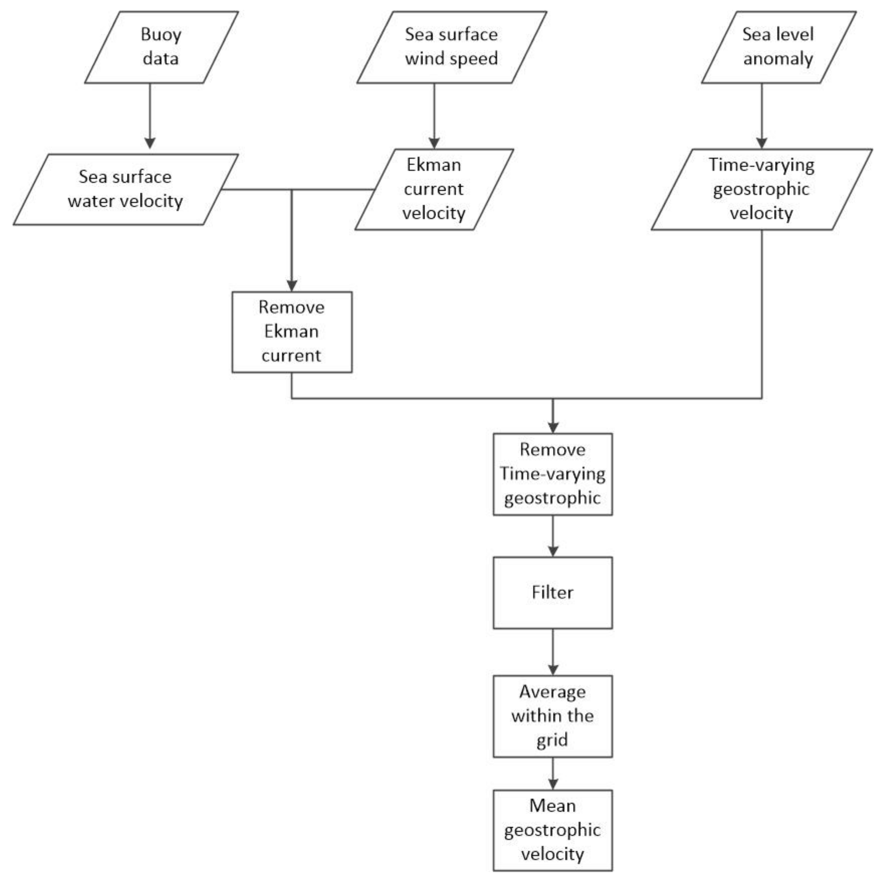
3.4. Drifting Buoy Data

Moreover, the geodetic MDTs modeled with and without the SAR altimetry data are assessed by using in situ buoy data in terms of geostrophic velocities. The buoy dataset was obtained from the Atlantic Ocean and Meteorological Laboratory (AOML, ftp://ftp.aoml.noaa.gov/phod/pub/buoydata (accessed on 25 May 2021)), where the quality of this dataset has been well controlled by using the Kriging method to provide 6-hour velocity measurements. We use the buoy data from 1993–2016 and the buoy-derived signals include geostrophic, tidal, Ekman, inertial, and high-frequency non-geostrophic currents. Since only the surface geostrophic currents can be derived from the geodetic MDT models, and we remove the non-geostrophic component and extract the geostrophic velocities from the buoy data for the comparison. To do this, we first remove the Ekman current from the buoy-derived currents, where the model developed by Rio et al. [32] is used, which was computed based on the data of the wind speed and wind stress. The time-varying geostrophic velocity should be deducted from the buoy-derived currents; it can be derived from SLA by equilibrium equation if we ignore the variability of the geoid. Moreover, a low-pass filter is applied to the residual buoy currents to remove the variability caused by tidal, inertial, and high-frequency non-geostrophic currents with the periods smaller than 3 days [54,55]. It is noticeable that the buoy data are scattered in space and time and often autocorrelated in both dimensions. In order to obtain the mean geostrophic velocity, a common approach is averaging the buoy data within spatial bins. The choice of bin size influences the accuracy of the geostrophic velocity. In this study, the bin size is chosen as 0.25° [55,56]. Moreover, the error of this dataset is estimated at each bin, which is given as the standard deviation of the observations divided by the square root of the number of observations in the bin. Generally, the estimated error of the buoy-derived geostrophic velocities is about 3–10 cm per second. The flow chart of extracting the geostrophic currents from the buoy data is seen in Figure 3.

4. Results

4.1. The Choice of the Estimation of Observation Error on MDT Modeling

In this study, we study several different schemes in order to choose a proper method for the error estimation of input datasets in the MOA method. To do this, different MDTs are modeled based on the error estimates derived from different schemes discussed in Section 2.2, with DTU18MSS as the mean sea surface model and GO_CONS_GCF_2_DIR_R6 as the gravity field model to compute the geoid height. We use three reference MDTs (i.e., CLS18MDT, DTU17MDT, CLS15MDT) to compute the error of the directly solved MDT. Similarly, from a set of four high-degree gravity field models (i.e., EGM2008, XGM2019e_2159, GECO, SGG_UGM_1), we calculate a set of informal geoid errors. Likewise, from three reference mean sea surface models, we calculate a set of informal mean sea surface errors. From these three sets, representing 735 possible combinations, we choose one of the best combinations as the error of the model. The estimated errors based on different schemes are seen in Figure 4, where different error estimates show heterogeneous patterns; however, the most significant errors concentrate over coastal areas. The associated statistics are shown in

Table 1. Statistics of the estimated errors of the observations from different schemes (Units: mm).

Study Area	Scheme	Min	Max	Mean	RMS
Coastal area of Japan	Scheme 1	111	810	371	397
	Scheme 2	116	830	375	397
	Scheme 3	115	791	376	395
Southeastern coastal area of China	Scheme 1	66	1315	208	274
	Scheme 2	64	1449	205	273
	Scheme 3	67	1135	220	272

. The results show that the root mean square (RMS) of the errors estimated by Scheme 3 is smaller than that estimated by Scheme 1 or Scheme 2. The mean of the error of the observations estimated by Scheme 3 is large than that estimated from Schemes 1 and 2. The reason is that the RMS of the difference is calculated in a 1° box, which may reduce the maximum value and increase the mean value when estimating the observation error by Scheme 3. The error estimated contains the reference model’s error, which may lead to the overestimation of the error.

We further compare these geodetic MDTs modeled by using different error estimates with independent synthetic/ocean data, where the mean value of all synthetic/ocean models (i.e., SODA3, ORAS5, CNES-CLS18MDT and Copernicus) is used as the reference MDT model, and we call it as the ocean data in the following study. This may provide sufficient independence and redundancy to allow more robust comparison, since the ocean models lack the formal error information, and the comparison with an individual ocean model may not have reliable results. Figure 5 shows the comparison results over the coastal area of Japan, where the figures in the top panel display the misfits between different geodetic MDTs and the ocean data. MDTs computed from the errors of observations estimated from Schemes 1–3 are denoted as MDT_JP_S1, MDT_JP_S2, and MDT_JP_S3, respectively. From Figure 5, we see that the differences between MDT_JP_S1/MDT_JP_S2 and the ocean data are larger than the ones derived from MDT_JP_S3, where the discrepancies between MDT_JP_S3 and the ocean data are extremely prominent over the regions of southwestern area of Japan. The statistics in

Table 2. Statistics of the differences between the estimated MDT and the ocean data (Units: mm).

Area	Scheme	Min	Max	RMS
Coastal area of Japan	Scheme 1	−465	250	123
	Scheme 2	−460	233	120
	Scheme 3	−445	224	115
Southeastern coastal area of China	Scheme 1	−454	154	80
	Scheme 2	−478	146	79
	Scheme 3	−454	149	77

show that the RMS of the differences between MDT_JP_S3 and the ocean data 115 mm, which is lower than the results derived from MDT_JP_S1 (MDT_JP_S2), by a magnitude of 8 mm (5 mm). The results suggest that the observations’ error computed from Scheme 3 may be a more realistic error estimate for the observations in the MOA method. Scheme 3 introduced many independent reference models to obtain the most reasonable combination to estimate the error of observation. Although there are errors in the reference models, which may lead to overestimation of the error of the observations, the use of Scheme 3 may derive more realistic errors, compared to the results derived from Scheme 1 (Scheme 2). Schemes 1 and 2 combine two different error estimation methods, both of them cannot obtain a reasonable result. In particular, the error of geoid is difficult to estimate. The error of geoid that is used in Scheme 2 is influenced by the selection of the reference gravity field models, which may lead to the overestimation of geoid error.

Moreover, the formal errors of these MDTs can be estimated by the MOA method, which are shown in the figures in the below panel of Figure 5. The formal errors of different MDTs concentrate over coastal regions, and this is in line with the comparison results with the ocean data, where the prominent misfits of these geodetic MDTs against the ocean data are located over the coastal areas. The formal errors of MDT_JP_S1 range from 11 to 30 mm, with an RMS value of 17 mm, and the most prominent errors are concentrated over the northern and eastern coast of Japan, reaching a magnitude of ~30 mm. The formal errors of MDT_JP_S2 is similar to MDT_JP_S1, with an RMS of 17 mm, while the formal errors of MDT_JP_S3 range from 11 to 31 mm, with an RMS of 15 mm, which is slightly smaller than that derived from MDT_JP_S1/MDT_JP_S2, by a magnitude of 2 mm. The formal errors of these MDTs show similar patterns with the differences between the estimated MDTs and ocean data. For example, both of them show larger differences in the southern coast of Japan (138°E, 34°N) and smaller differences/errors in the southwestern coast of Japan (129°E, 32°N). However, on the northeastern coast of Japan, the formal errors and the differences between the modeled MDTs and ocean data show different patterns, the formal errors are large where the differences are small. The reason is that the formal errors are influenced by the error of the observations. This generally agrees with the results derived from the comparisons with the ocean data, where MDT modeled from the observations’ error computed from Scheme 3 shows a better fit with the ocean data, compared to the results derived from the other two schemes.

MDTs computed from the errors of observations estimated from Schemes 1–3 in the southeastern coastal area of China are denoted as MDT_SECN_S1, MDT_SECN_S2, and MDT_SECN_S3, respectively. Similar to the case over Japan, the misfits between the geodetic MDT computed from the errors of observations estimated from Scheme 3 are smaller than those derived from Scheme 1 (Scheme 2); see the figures in the top panel of Figure 6. The discrepancies of MDT_SECN_S3 against the ocean data are extremely large along the coast of Guangdong in China, which reach a magnitude exceeding 30 cm. The reason may be due to the overestimation of the error of the observation estimated by Scheme 1 (Scheme 2), which estimates errors by comparing the errors derived from two method and induce more errors of the reference models. Similar as the results derived from the regions over Japan, the solution derived from the errors of observations estimated from Scheme 3 shows a better fit with the ocean data than those derived from the other two schemes. The statistics in Table 2 show that the RMS of the difference between MDT_SECN_S3 and the ocean data is 77 mm, which is 2 mm lower than that derived from MDT_SECN_S2 and 3 mm lower than the derived from MDT_SECN_S1. The formal errors of the estimated MDTs are shown in the figures in the below panel of Figure 6. The formal errors are large around Taiwan. The RMS of the error of MDT_SECN_S3 is 13 mm, which is ~3 mm lower than that of MDT_SECN_S2 and MDT_SECN_S1. The results suggest that Scheme 3 is more appropriate to estimate the observation errors on MDT modeling since MDT modeled by using the observations’ errors computed from Scheme 3 derives better results, and in the following study, the observations’ errors are estimated from Scheme 3.

4.2. Assessment of MDTs Modeled with SAR Altimetry Data

We further investigate the performances of using the SAR-based mean sea surface models in local MDT recovery, and MDT solutions modeled with and without SAR altimetry data are compared and assessed. Three mean sea surface models, i.e., DTU15MSS, DTU18MSS, DTU21MSS, are used. As we mentioned in Section 3.1, no SAR altimetry was used in DTU15MSS over these two study areas, while the 3-year SAR altimetry data from Sentinel-3A was used in DTU18MSS and the SAR data from Sentinel-3A and Sentinel-3B data were used in DTU21MSS. The figures in the top panel of Figure 7 show the differences between MDTs modeled from different mean sea surface models and the ocean data over the coast of Japan. In the northern coastal area of Japan (134°E, 34°N) and the southern coast of Japan (138°E, 33.5°N), MDT modeled by DTU21MSS, which uses more SAR data, is better than the one modeled by DTU15MSS/DTU18MSS. The statistics in

Table 3. Statistics of the differences between the ocean data and the geodetic MDTs modeled from different MSS models (Units: mm).

Area	MSS Model	Min	Max	RMS
Coastal area of Japan	DTU15MSS	−448	228	116
	DTU18MSS	−445	224	115
	DTU21MSS	−435	220	111
Southeastern coastal area of China	DTU15MSS	−450	144	78
	DTU18MSS	−454	149	77
	DTU21MSS	−437	140	70

show that the RMS of the differences between MDT modeled from DTU15MSS and the ocean data is 116 mm; however, this RMS value almost stays unchanged when the DTU18MSS is used in MDT modeling, although the computation of DTU18MSS included 3 years of SAR altimetry data from Sentinel-3A, whereas the RMS of the differences between MDT modeled from DTU21MSS and the ocean data is 111 mm, which is smaller than that derived from DTU18MSS (DTU15MSS), by a magnitude of 4 mm (5 mm). The better fit of MDT modeled from DTU21MSS with the ocean data is mainly attributed to the use of more high-quality SAR altimetry data and an updated waveform retracker (the SAMOSA+ physical retracker) in the data preprocessing procedures. Moreover, the formal errors of MDT modeled from DTU21MSS range from 11 to 30 mm, and the RMS value is 14 mm, while the RMS of the formal errors of MDT computed from DTU18MSS (DTU15MSS) is ~15 mm (15 mm), which is marginally larger than the value derived from DTU21MSS.

Figure 8 shows the assessment of MDTs modeled from different mean sea surface models over the southern coast of China, and we see that the application of DTU21MSS in MDT recovery reduces the misfits against the ocean data, compared to the results derived from DTU15MSS/DTU18MSS, see the figures in the top panel. By using the DTU21MSS, the improvements are mainly seen in the Taiwan Strait and the north of Taiwan, compared to MDT modeled from DTU15MSS/DTU18MSS. The RMS of the differences between MDT modeled from DTU21MSS and the ocean data is 70 mm, while this value changes to 78/77 mm when MDT modeled from DTU15MSS/DTU18MSS is assessed with the ocean data, with an increase of ~8/7 mm. Moreover, the figures in the lower panel of Figure 8 show the formal errors of MDTs modeled from different mean sea surface models, the formal errors of these MDTs range from 14 to 22 mm. The RMS of the formal errors of MDT derived from DTU21MSS is 9 mm, while the RMS of the formal errors of MDT derived from DTU15MSS/DTU18MSS is 16/13 mm, which is slightly larger. These results show that the use of the mean sea surface model computed with high-quality SAR altimetry data can improve MDT modeling over coastal regions, which may improve the coast MDT by a magnitude of several millimeters, compared to MDT computed with the mean sea surface model without SAR altimetry data.

MDTs estimated by the MOA method are shown in Figure 9. The prior errors of MDT are estimated by Scheme 3. The input models are DTU21MSS and the DIRR6 geoid model. In Figure 9a, MDT ranges from 115 to 1442 mm in the coast of Japan. The large signals are shown in the area of the Kuroshio current (130°E, 30°N), whereas the small signals are observed in the coastal zone. In Figure 9b, MDT ranges from 248 to 1218 mm in the southeastern coastal area of China. The large signals are shown in the coastal area of Guangdong (114°E, 21°N), while the smallest signals are seen in the north of Taiwan.

5. Discussions

In order to further assess the geodetic MDTs modeled from the different altimeter data, the in situ buoy data are used as the control data. The geostrophic velocities can be obtained from MDT gradients at the ocean surface, and the used equations are seen in, for example, Hwang and Sung [57]. The geostrophic velocities computed from the geodetic MDTs are interpolated to the point of the buoy data and the differences between them are shown in Figure 10 and Figure 11. From Figure 10, we can see that the improvements are mainly shown in the northern coast of Japan and the southern coast of Japan for the geostrophic velocities computed from MDT modeled with DTU21MSS, compared to the ones computed from DTU15MSS/DTU18MSS. In Figure 11, we see that the zonal (meridional) geostrophic velocities computed from MDT modeled with DTU21MSS show better results over the coast of Guangdong and the Taiwan Strait, compared to the results computed from DTU15MSS/DTU18MSS. The statistics of the differences between MDT-derived geostrophic velocities and the buoy data are shown in

Table 4. Statistics of the differences of the geostrophic velocities between the buoy data and the values derived from MDT solutions computed from different MSS models (Units: mm/s) (u: zonal velocities; v: meridian velocities).

Study Area	MSS Model	Geostrophic Velocities	Min	Max	RMS
Coastal area of Japan	DTU15MSS	u	−657	906	179
		v	−400	711	141
	DTU18MSS	u	−650	907	178
		v	−401	709	141
	DTU21MSS	u	−651	901	174
		v	−406	714	140
Southeastern coastal area of China	DTU15MSS	u	−267	678	101
		v	−335	555	107
	DTU18MSS	u	−260	676	99
		v	−326	553	105
	DTU21MSS	u	−251	664	97
		v	−325	551	105

, from which it can be seen that the RMS of the differences between the zonal (meridional) velocities computed from MDT modeled with DTU21MSS and the in situ data is 174 mm/s (140 mm/s), which is 5 mm/s (1 mm/s) lower than that of the velocities computed from MDT modeled with DTU15MSS over the coast of Japan. The RMS of the differences between the zonal (meridional) geostrophic velocities derived from MDT modeled with DTU21MSS and the buoy data is 97 mm/s (105 mm/s), which is about 4 mm/s (2 mm/s) lower than that of the velocities computed from DTU15MSS over the coast of southeastern China. These results indicate that the use of SAR altimetry data improves the accuracy of mean sea surface, and the improvement of the mean sea surface model can contribute to MDT and geostrophic current modeling over coastal areas.

As mentioned above, the comparison with ocean data and in situ buoy data has proven that MDT based on the MSS with SAR altimetry data outperforms that without SAR altimetry data. The reason is that the altimetry satellite operated in SAR mode can obtain more accurate signals over coastal area. The conventional radar altimeter data are seriously degraded in coastal zones due to the signal contamination by land. Therefore, the more accurate mean sea surface model can be obtained in coastal area, and MDT can be further improved. However, from the statistics of the results, the improvement of MDT with SAR altimetry data is limited. This result may be caused by many reasons. We sum up the following three possible reasons:

(1)

The improvement in the mean sea surface model with SAR altimetry data is limited. The differences between DTU21MSS and DTU18MSS (DTU15MSS) are less than 1 cm in most of the study area. Therefore, the improvement of MDT with SAR altimetry data is limited.

(2)

The accuracy and resolution of the reference model that we used for comparison are limited. The accuracy of ocean data ranges from several centimeters to decimeter level. The resolution of ocean data is 15′. The improvement of MDT with SAR altimetry data cannot be well reflected in coastal area.

(3)

The geoid model we used is a recently released GRACE/GOCE combined model (DIRR6). The contribution of GOCE is focus on the scale of about 80 km; the shorter scale of signals cannot be reflected in this geoid model. However, the improvement in the mean sea surface model with SAR altimetry data concentrates upon the signals of short scale (tens of kilometers). Moreover, the accuracy and resolution of estimated MDT are mainly restricted by the geoid model. Therefore, the estimated MDT may lack the short scale signals, which leads to the limited improvement of MDT-modeled with SAR altimetry data.

6. Conclusions

We focused on coastal MDT refinement by using SAR altimetry data, and the effects introduced by the SAR altimetry data are validated and quantified. We modeled the local MDT based on the multivariate objective analysis (MOA) method, and independent ocean reanalysis data and buoy data were used for model assessment, based on which MDTs modeled with and without the SAR altimetry data were discriminated. The numerical results over the coast of Japan and southeastern China showed that:

(1)

The informal approach we used in this study may be suitable for the error estimate of the observations of the multivariate objective analysis method. This approach is particularly useful when the formal errors of the geoid or MDT are difficult to estimate, even over coastal regions, where the errors of input datasets for MDT modeling are hard to model.

(2)

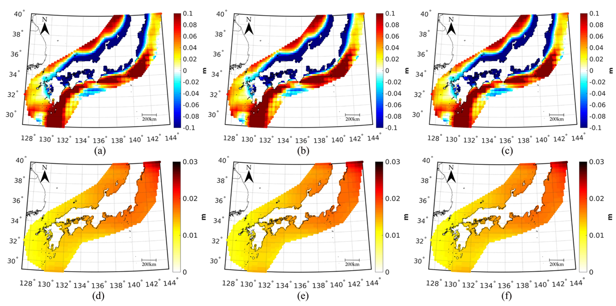
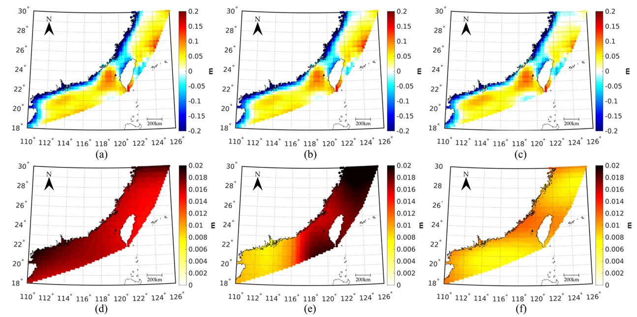
The use of the mean sea surface models computed with high-quality SAR altimetry data improves MDT modeling over coastal regions, by a magnitude of about several millimeters. The RMS of the differences between MDT modeled from DTU21MSS (with SAR altimetry data from Sentinel-3A/3B) and ocean data is 8 mm (5 mm) lower than that computed from DTU15MSS (without SAR altimetry data) over the coast of southeastern China (Japan).

(3)

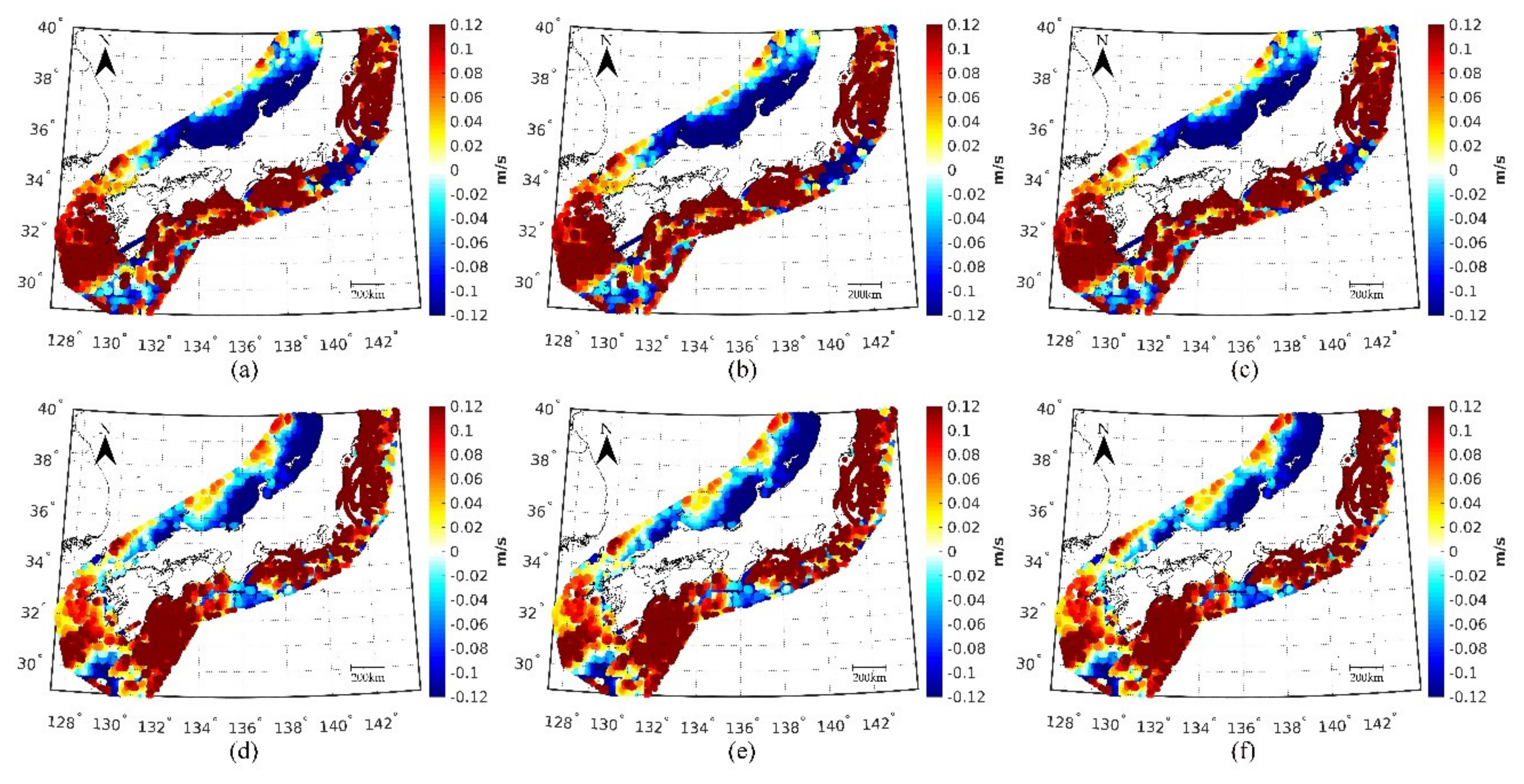
Moreover, the use of a SAR-based mean sea surface model improves the computation of local geostrophic velocities, compared with the values computed from the mean sea surface modeled without the SAR altimetry data. The RMS of the differences between the zonal (meridian) velocities derived from MDT modeled with DTU21MSS and the in situ buoy data were 5 mm/s (1 mm/s) less than the results derived from DTU15MSS over the coast of Japan, which is 4 mm/s (2 mm/s) less than the results derived from DTU15MSS over the coast of southeastern China.

References

1. Lyu, K.; Yang, X.-Y.; Zheng, Q.; Wang, D.; Hu, J. Intraseasonal Variability of the Winter Western Boundary Current in the South China Sea Using Satellite Data and Mooring Observations. IEEE J. Sel. Top. Appl. Earth Obs. Remote. Sens. 2016, 9, 5079–5088. [Google Scholar] [CrossRef]
2. Li, J.; Wang, G.; Xue, H.; Wang, H. A simple predictive model for the eddy propagation trajectory in the northern South China Sea. Ocean Sci. 2019, 15, 401–412. [Google Scholar] [CrossRef] [Green Version]
3. Lin, H.; Thompson, K.R.; Huang, J.; Véronneau, M. Tilt of mean sea level along the Pacific coasts of North America and Japan. J. Geophys. Res. Oceans 2015, 120, 6815–6828. [Google Scholar] [CrossRef] [Green Version]
4. Filmer, M.S.; Hughes, C.W.; Woodworth, P.L.; Featherstone, W.E.; Bingham, R.J. Comparison between geodetic and oceanographic approaches to estimate mean dynamic topography for vertical datum unification: Evaluation at Australian tide gauges. J. Geod. 2018, 12, 1413–1437. [Google Scholar] [CrossRef] [Green Version]
5. Featherstone, W.E.; Filmer, M.S. The north-south tilt in the Australian Height Datum is explained by the ocean’s mean dynamic topography. J. Geophys. Res. Oceans 2012, 117, C08035. [Google Scholar] [CrossRef] [Green Version]
6. Wu, Y.; Abulaitijiang, A.; Featherstone, W.E.; McCubbine, J.C.; Andersen, O.B. Coastal gravity field refinement by combining airborne and ground-based data. J. Geod. 2019, 93, 2569–2584. [Google Scholar] [CrossRef]
7. Xu, L.; He, Y.; Huang, W.; Cui, S. A multi-dimensional integrated approach to assess flood risks on a coastal city, induced by sea-level rise and storm tides. Environ. Res. Lett. 2016, 11, 014001. [Google Scholar] [CrossRef] [Green Version]
8. Smith, A.J.; Kirwan, M.L. Sea Level-Driven Marsh Migration Results in Rapid Net Loss of Carbon. Geophys. Res. Lett. 2021, 48, e2021GL092420. [Google Scholar] [CrossRef]
9. Weisse, R.; Dailidienė, I.; Hünicke, B.; Kahma, K.; Madsen, K.; Omstedt, A.; Parnell, K.; Schöne, T.; Soomere, T.; Zhang, W.; et al. Sea level dynamics and coastal erosion in the Baltic Sea region. Earth Syst. Dyn. 2021, 12, 871–898. [Google Scholar] [CrossRef]
10. Genchi, S.A.; Vitale, A.J.; Perillo, G.M.E.; Seitz, C.; Delrieux, C.A. Mapping Topobathymetry in a Shallow Tidal Environment Using Low-Cost Technology. Remote Sens. 2020, 12, 1394. [Google Scholar] [CrossRef]
11. Andersen, O.B.; Knudsen, P. DNSC08 mean sea surface and mean dynamic topography models. J. Geophys. Res. Space Phys. 2009, 114, 1–12. [Google Scholar] [CrossRef]
12. Schaeffer, P.; Faugére, Y.; Legeais, J.F.; Ollivier, A.; Guinle, T.; Picot, N. The CNES_CLS11 Global Mean Sea Surface Computed from 16 Years of Satellite Altimeter Data. Mar. Geod. 2012, 35, 3–19. [Google Scholar] [CrossRef]
13. Tapley, B.D.; Bettadpur, S.; Watkins, M.; Reigber, C. The gravity recovery and climate experiment: Mission overview and early results. Geophys. Res. Lett. 2004, 31, L09607. [Google Scholar] [CrossRef] [Green Version]
14. Tapley, B.; Chambers, D.P.; Bettadpur, S.; Ries, J.C. Large scale ocean circulation from the GRACE GGM01 Geoid. Geophys. Res. Lett. 2003, 30, 2163. [Google Scholar] [CrossRef] [Green Version]
15. Pail, R.; Bruinsma, S.; Migliaccio, F.; Förste, C.; Goiginger, H.; Schuh, W.-D.; Höck, E.; Reguzzoni, M.; Brockmann, J.M.; Abrikosov, O.; et al. First GOCE gravity field models derived by three different approaches. J. Geod. 2011, 85, 819–843. [Google Scholar] [CrossRef] [Green Version]
16. Pail, R.; Goiginger, H.; Schuh, W.-D.; Hock, E.; Brockmann, J.M.; Fecher, T.; Gruber, T.; Mayer-Gürr, T.; Kusche, J.; Jäggi, A.; et al. Combined satellite gravity field modelGOCO01Sderived from GOCE and GRACE. Geophys. Res. Lett. 2010, 37. [Google Scholar] [CrossRef]
17. Bruinsma, S.L.; Förste, C.; Abrikosov, O.; Marty, J.-C.; Rio, M.-H.; Mulet, S.; Bonvalot, S. The new ESA satellite-only gravity field model via the direct approach. Geophys. Res. Lett. 2013, 40, 3607–3612. [Google Scholar] [CrossRef] [Green Version]
18. Bingham, R.J.; Knudsen, P.; Andersen, O.; Pail, R. An initial estimate of the North Atlantic steady-state geostrophic circulation from GOCE. Geophys. Res. Lett. 2011, 38, L01606. [Google Scholar] [CrossRef] [Green Version]
19. Volkov, D.L.; Zlotnicki, V. Performance of GOCE and GRACE-derived mean dynamic topographies in resolving Antarctic Circumpolar Current fronts. Ocean Dyn. 2012, 62, 893–905. [Google Scholar] [CrossRef]
20. Deng, X.; Featherstone, W.E. A coastal retracking system for satellite radar altimeter waveforms: Application to ERS-2 around Australia. J. Geophys. Res. Oceans 2006, 111, C06012. [Google Scholar] [CrossRef] [Green Version]
21. Andersen, O.B.; Scharroo, R. Range and geophysical corrections in coastal regions: And implications for mean sea surface determination. In Coastal Altimetry; Benveniste, J., Ed.; Springer: Berlin/Heidelberg, Germany, 2011. [Google Scholar] [CrossRef]
22. Abulaitijiang, A.; Andersen, O.B.; Stenseng, L. Coastal sea level from inland CryoSat-2 interferometric SAR altimetry. Geophys. Res. Lett. 2015, 42, 1841–1847. [Google Scholar] [CrossRef]
23. Dinardo, S.; Fenoglio-Marc, L.; Buchhaupt, C.; Becker, M.; Scharroo, R.; Joana Fernandes, M.; Benveniste, J. Coastal SAR and PLRM altimetry in German bight and west Baltic sea. Adv. Space Res. 2017, 62, 1371–1404. [Google Scholar] [CrossRef]
24. Landy, J.C.; Petty, A.A.; Tsamados, M.; Stroeve, J.C. Sea Ice Roughness Overlooked as a Key Source of Uncertainty in CryoSat-2 Ice Freeboard Retrievals. J. Geophys. Res. Oceans 2020, 125, e2019JC015820. [Google Scholar] [CrossRef]
25. Gómez-Enri, J.; Vignudelli, S.; Cipollini, P.; Coca, J.; González, C. Validation of CryoSat-2 SIRAL sea level data in the eastern continental shelf of the Gulf of Cadiz (Spain). Adv. Space Res. 2018, 62, 1405–1420. [Google Scholar] [CrossRef] [Green Version]
26. Idžanović, M.; Ophaug, V.; Andersen, O.B. Coastal sea level from CryoSat-2 SARIn altimetry in Norway. Adv. Space Res. 2018, 62, 1344–1357. [Google Scholar] [CrossRef] [Green Version]
27. Buchhaupt, C.; Fenoglio, L.; Becker, M.; Kusche, J. Impact of vertical water particle motions on focused SAR altimetry. Adv. Space Res. 2021, 68, 853–874. [Google Scholar] [CrossRef]
28. Bonnefond, P.; Laurain, O.; Exertier, P.; Boy, F.; Guinle, T.; Picot, N.; Labroue, S.; Raynal, M.; Donlon, C.; Féménias, P.; et al. Calibrating the SAR SSH of Sentinel-3A and CryoSat-2 over the Corsica Facilities. Remote Sens. 2018, 10, 92. [Google Scholar] [CrossRef] [Green Version]
29. Donlon, C.; Berruti, B.; Buongiorno, A.; Ferreira, M.H.; Féménias, P.; Frerick, J.; Goryl, P.; Klein, U.; Laur, H.; Mavrocordatos, C.; et al. The Global Monitoring for Environment and Security (GMES) Sentinel-3 mission. Remote Sens. Environ. 2012, 120, 37–57. [Google Scholar] [CrossRef]
30. Bretherton, F.P.; Davis, R.E.; Fandry, C.B. A technique for objective analysis and design of oceanographic experiments applied to MODE-73. Deep Sea Res. Oceanogr. Abstr. 1976, 23, 559–582. [Google Scholar] [CrossRef]
31. Rio, M.H.; Guinehut, S.; Larnicol, G. New CNES-CLS09 global mean dynamic topography computed from the combination of GRACE data, altimetry, and in situ measurements. J. Geophys. Res. Oceans 2011, 116, C07018. [Google Scholar] [CrossRef]
32. Rio, M.H.; Hernandez, F.A. Mean dynamic topography computed over the world ocean from altimetry, in situ measurements, and a geoid model. J. Geophys. Res. Oceans 2004, 109, C12032. [Google Scholar] [CrossRef] [Green Version]
33. Rio, M.-H.; Mulet, S.; Picot, N. Beyond GOCE for the ocean circulation estimate: Synergetic use of altimetry, gravimetry, and in situ data provides new insight into geostrophic and Ekman currents. Geophys. Res. Lett. 2014, 41, 8918–8925. [Google Scholar] [CrossRef]
34. Wu, Y.; Huang, J.; Shi, H.; He, X. Mean Dynamic Topography Modeling Based on Optimal Interpolation from Satellite Gravimetry and Altimetry Data. Appl. Sci. 2021, 11, 5286. [Google Scholar] [CrossRef]
35. Arhan, M.; De Verdiére, A.C. Dynamics of eddy motions in the eastern North Atlantic. J. Phys. Oceanogr. 1985, 15, 153–170. [Google Scholar] [CrossRef] [Green Version]
36. Balmino, G. Efficient propagation of error covariance matrices of gravitational models: Application to GRACE and GOCE. J. Geod. 2009, 83, 989–995. [Google Scholar] [CrossRef]
37. Bingham, R.J.; Haines, K.; Lea, D.J. How well can we measure the ocean’s mean dynamic topography from space? J. Geophys. Res. Oceans 2014, 119, 3336–3356. [Google Scholar] [CrossRef] [Green Version]
38. Oka, E.; Kawabe, M. Dynamic Structure of the Kuroshio South of Kyushu in Relation to the Kuroshio Path Variations. J. Geophys. Res. 2003, 59, 595–608. [Google Scholar] [CrossRef]
39. Andersen, O.; Knudsen, P.; Stenseng, L. A New DTU18 MSS Mean Sea Surface–Improvement from SAR Altimetry. In Proceedings of the 25 Years of Progress in Radar Altimetry Symposium, Ponta Delgada, Portugal, 24–29 September 2018. [Google Scholar]
40. Zhu, C.; Liu, X.; Guo, J.; Yu, S.; Niu, Y.; Yuan, J.; Gao, Y. Sea Surface Heights and Marine Gravity Determined from SARAL/AltiKa Ka-band Altimeter Over South China Sea. Pure Appl. Geophys. 2021, 178, 1513–1527. [Google Scholar] [CrossRef]
41. Jiang, L.; Nielsen, K.; Dinardo, S.; Andersen, O.B.; Bauer-Gottwein, P. Evaluation of Sentinel-3 SRAL SAR altimetry over Chinese rivers. Remote Sens. Environ. 2020, 237, 111546. [Google Scholar] [CrossRef]
42. Andersen, O.B.; Abulaitijiang, A.; Zhang, S.; Rose, S.K. A new high resolution Mean Sea Surface (DTU21MSS) for improved sea level monitoring. In Proceedings of the EGU General Assembly 2021, Online, 19–30 April 2021. EGU21-16084. [Google Scholar] [CrossRef]
43. Förste, C.; Abrykosov, O.; Bruinsma, S.; Dahle, C.; König, R.; Lemoine, J.M. ESA’s Release 6 GOCE Gravity Field Model by Means of the Direct Approach Based on Improved Filtering of the Reprocessed Gradients of the Entire Mission; Data Publication; GFZ Data Services: Potsdam, Germany, 2019. [Google Scholar] [CrossRef]
44. Gruber, T. GOCE Release 6 Products and Performance. In Proceedings of the 27th IUGG General Assembly, Montreal, QC, Canada, 8–18 July 2019. [Google Scholar]
45. Carton, J.A.; Chepurin, G.A.; Chen, L. SODA3: A New Ocean Climate Reanalysis. J. Clim. 2018, 31, 6967–6983. [Google Scholar] [CrossRef]
46. Zuo, H.; Balmaseda, M.A.; Tietsche, S.; Mogensen, K.; Mayer, M. The ECMWF operational ensemble reanalysis–analysis system for ocean and sea ice: A description of the system and assessment. Ocean Sci. 2019, 15, 779–808. [Google Scholar] [CrossRef] [Green Version]
47. Mulet, S.; Rio, M.-H.; Etienne, H.; Artana, C.; Cancet, M.; Dibarboure, G.; Feng, H.; Husson, R.; Picot, N.; Provost, C.; et al. The new CNES-CLS18 global mean dynamic topography. Ocean Sci. 2021, 17, 789–808. [Google Scholar] [CrossRef]
48. Mayer-Gürr, T.; Kvas, A.; Klinger, B.; Rieser, D.; Zehentner, N.; Pail, R. The combined satellite gravity field model GOCO05s. In Proceedings of the EGU General Assembly, Online, 12–17 April 2015. [Google Scholar]
49. Bingham, R.J.; Haines, K. Mean dynamic topography: Intercomparisons and errors. Philos. Trans. R. Soc. A Math. Phys. Eng. Sci. 2006, 364, 903–916. [Google Scholar] [CrossRef] [PubMed]
50. Ophaug, V.; Breili, K.; Gerlach, C. A comparative assessment of coastal mean dynamic topography in Norway by geodetic and ocean approaches. J. Geophys. Res. Oceans 2015, 120, 7807–7826. [Google Scholar] [CrossRef] [Green Version]
51. Idžanović, M.; Ophaug, V.; Andersen, O.B. The coastal mean dynamic topography in Norway observed by CryoSat-2 and GOCE. Geophys. Res. Lett. 2017, 44, 5609–5617. [Google Scholar] [CrossRef] [Green Version]
52. Shi, H.; He, X.; Wu, Y.; Huang, J. The parameterization of mean dynamic topography based on the Lagrange basis functions. Adv. Space Res. 2020, 66. [Google Scholar] [CrossRef]
53. Wu, Y.; Abulaitijiang, A.; Andersen, O.B.; He, X.; Luo, Z.; Wang, H. Refinement of Mean Dynamic Topography Over Island Areas Using Airborne Gravimetry and Satellite Altimetry Data in the Northwestern South China Sea. J. Geophys. Res. Solid Earth 2021, 126, e2021JB021805. [Google Scholar] [CrossRef]
54. Johnson, G.C. The Pacific Ocean Subtropical cell surface limb. Geophys. Res. Lett. 2001, 28, 1771–1774. [Google Scholar] [CrossRef]
55. Lumpkin, R.; Johnson, G.C. Global ocean surface velocities from drifters: Mean, variance, El Niño-Southern Oscillation response, and seasonal cycle. J. Geophys. Res. Oceans 2013, 118, 2992–3006. [Google Scholar] [CrossRef]
56. Uchida, H.; Imawaki, S. Eulerian mean surface velocity field derived by combining drifter and satellite altimeter data. Geophys. Res. Lett 2003, 30, 33. [Google Scholar] [CrossRef]
57. Hwang, C.; Chen, S.-A. Circulations and eddies over the South China Sea derived from TOPEX/Poseidon altimetry. J. Geophys. Res. Space Phys. 2000, 105, 23943–23965. [Google Scholar] [CrossRef]
Figure 1. Flow chart of MDT modeling form the MOA method. The flow chart of observations error estimation is shown in the dashed rectangle.
Remotesensing 14 00240 g001
Figure 2. The study areas, which are enclosed in the red dashed polygon. The solid blue line represents the Kuroshio current, and the solid yellow line shows the Tsushima current.
Remotesensing 14 00240 g002
Figure 3. The flow chart of extracting geostrophic velocities from buoy data.
Remotesensing 14 00240 g003
Figure 4. The estimated errors of the observations calculated from (a) Scheme 1, (b) Scheme 2, and (c) Scheme 3 over the coast of Japan; the estimated error of the observations computed from (d) Scheme 1, (e) Scheme 2, and (f) Scheme 3 over the coast of southeastern China.
Remotesensing 14 00240 g004
Figure 5. Differences between the modeled MDT derived from (a) Scheme 1, (b) Scheme 2, and (c) Scheme 3 and the ocean data. (df) Corresponding formal errors estimated from the MOA over the coastal area of Japan.
Remotesensing 14 00240 g005
Figure 6. Differences between the estimated MDT by (a) Scheme 1, (b) Scheme 2, and (c) Scheme 3 and reference MDT. (df) Corresponding formal errors estimated from MOA over coastal southeastern China.
Remotesensing 14 00240 g006
Figure 7. Differences between MDT modeled from (a) DTU15MSS, (b) DTU18MSS, and (c) DTU21MSS and the ocean data; (df) show the corresponding formal errors over the coast of Japan.
Remotesensing 14 00240 g007
Figure 8. Differences between MDT modeled from (a) DTU15MSS, (b) DTU18MSS, (c) DTU21MSS and the ocean data; (df) show the corresponding formal errors over the coast of southeastern China.
Remotesensing 14 00240 g008
Figure 9. The estimated MDTs over (a) the coastal area of Japan and (b) southeastern coastal area of China.
Remotesensing 14 00240 g009
Figure 10. Differences between the zonal (meridian) geostrophic velocities derived from the buoy data and the values computed from MDTs derived from different MSS models over the coast of Japan. (ac) and (df) represent the results of zonal and meridian velocities, respectively, and the left, middle, and right figures are the results derived from DTU15MSS, DTU18MSS, and DTU21MSS, respectively.
Remotesensing 14 00240 g010
Figure 11. Differences between the zonal (meridian) geostrophic velocities derived from the buoy data and the values computed from MDTs derived from different MSS models over coast of southeastern China. (ac) and (df) represent the results of zonal and meridian velocities, respectively, and the left, middle, and right figures are the results derived from DTU15MSS, DTU18MSS, and DTU21MSS, respectively.
Remotesensing 14 00240 g011