Article

Reconstructing High-Precision Coral Reef Geomorphology from Active Remote Sensing Datasets: A Robust Spatial Variability Modified Ordinary Kriging Method

1
School of Surveying and Geo-Informatics, Shandong Jianzhu University, Jinan 250101, China
2
Academy of Agricultural Planning and Engineering, Ministry of Agriculture and Rural Affairs, Beijing 100125, China
3
State Key Laboratory of Resources and Environmental Information System, Institute of Geographic Sciences and Natural Resources Research, Chinese Academy of Sciences, Beijing 100101, China
4
Guangxi Laboratory on the Study of Coral Reefs in the South China Sea, Guangxi University, Nanning 530004, China
*
Author to whom correspondence should be addressed.
Shared first authorship.
Submission received: 30 October 2021 / Revised: 18 December 2021 / Accepted: 3 January 2022 / Published: 6 January 2022
(This article belongs to the Special Issue GIS and RS in Ocean, Island and Coastal Zone)

Abstract

:
Active remote sensing technology represented by multi-beam and lidar provides an important approach for the effective acquisition of underwater coral reef geomorphological information. A spatially continuous surface model of coral reef geomorphology reconstructed from active remote sensing datasets can provide important geomorphological parameters for the research of coral reef geomorphological and ecological changes. However, the surface modeling methods commonly used in previous studies, such as ordinary kriging (OK) and natural neighborhood (NN), often represent a “smoothing effect”, which causes the strong spatial variability of coral reefs to be imprecisely reflected by the reconstructed surfaces, thus affecting the accurate calculation of subsequent geomorphological parameters. In this study, a spatial variability modified OK (OK-SVM) method is proposed to reduce the impact of the “smoothing effect” on the high-precision reconstruction of the complex geomorphology of coral reefs. The OK-SVM adopts a collaborative strategy of global parameter transformation, local residual correction, and extremum correction to modify the spatial variability of the reconstructed model, while maintaining high local accuracy. The experimental results show that the OK-SVM has strong robustness to spatial variability modification. This method was applied to the geomorphological reconstruction of the northern area of a coral atoll in the Nansha Islands, South China Sea, and the performance was compared with that of OK and NN. The results show that OK-SVM has higher numerical accuracy and attribute accuracy in detailed morphological fidelity, and is more adaptable in the geomorphological reconstruction of coral reefs with strong spatial variability. This method is relatively reliable for achieving high-precision reconstruction of complex geomorphology of coral reefs from active remote sensing datasets, and has potential to be extended to other geomorphological reconstruction applications.

1. Introduction

Global environmental changes have posed a strong threat to coral reef ecosystems, with increasing coral reef bleaching and death [1,2,3,4,5,6,7]. Especially in the process of exploitation and utilization of coral reef resources, human beings have caused continuous and strong disturbances to coral reef ecosystems, resulting in a significant trend of degradation of coral reef geomorphology and habitat [8,9,10,11]. Therefore, it is urgent to carry out investigation and exploration of coral reef geomorphology and continuously obtain information on coral reef geomorphology and its changes to provide data and a decision-making basis for coral reef research, development, utilization, and protection.
Remote sensing technology is regarded as the most promising way to carry out large-scale coral reef geomorphology survey and exploration [12,13,14,15,16], mainly including passive remote sensing and active remote sensing. Since there is no dedicated satellite for coral reef monitoring, most of the data used in passive remote sensing are mainly the optical images of airborne aerial platforms or land satellite platforms [17], and they are susceptible to the influence of the atmosphere and the water column [18]. Active remote sensing datasets of multi-beam and lidar are independent of solar radiation sources, which can make up for the limitations imposed by water transparency on passive remote sensing, and has been applied to the survey and evaluation of coral reef geomorphology [19,20,21,22]. Particularly, active remote sensing datasets provide the opportunity to conduct the geomorphological reconstruction of coral reefs. The parameters that characterize the spatial variability of coral reefs, such as surface roughness and morphological complexity, can then be derived, which is of great importance for the study of coral reef geomorphological and ecological changes [23,24,25,26]. Therefore, for coral reef geomorphology with strong spatial variability, a high-precision, spatially continuous geomorphological surface is the key to accurately obtain geomorphological parameters.
At present, the surface modeling methods based on spatial interpolation are the main way to reconstruct the spatially continuous surface model of coral reef geomorphology from discrete lidar and multi-beam datasets [27,28]. The choice of spatial interpolation method often has a direct impact on the accuracy of surface modeling [29,30,31], which in turn will have impacts on the accuracy of various parameters derived from the surface model. In the existing studies, there are some direct empirical choices of kriging [32], natural neighborhood (NN) [33], and triangulation linear interpolation [21] to reconstruct the surface model of coral reef geomorphology, but these lack consideration for geomorphic adaptation. In contrast, other studies have conducted a comparison of the performance of spatial interpolation methods and given an analysis of adaptability for coral reef geomorphology. For example, Leon and Woodroffe [22] argue that the global interpolation method is clearly inappropriate in the geomorphological reconstruction of coral reefs with complex morphological features and that ordinary kriging (OK) is superior to radial basis function (RBF) for a given data distribution. In addition, Coleman et al. [28] compared the accuracy of NN, inverse distance weight (IDW), spline and OK in the reconstruction of coral reef geomorphology when there are gaps in the datasets. They believed that NN is unable to reproduce extreme surface morphologies such as peaks and valleys; the reconstructed surface model is smoother and more natural, with the best performance, followed by OK [28]. Similarly, Leon et al. [34] compared kriging and NN, and believed that NN preserves the range of the original values and generates a smooth and visually effective coral reef geomorphological surface, which is suitable for further geomorphological analysis.
Although NN and kriging have relatively excellent numerical accuracy performance in the studies of coral reef geomorphological reconstruction, it should be noted that coral reef geomorphology has strong spatial variability, especially for the reef flat, with diverse species composition and extremely complex geomorphology. Important parameters such as morphological complexity and roughness derived from the relatively “smooth” surface model generated by NN may not be able to accurately reflect the changes of the coral reef geomorphology or ecology. Similarly, kriging methods, especially OK, as a widely used and reliable interpolation method, lack sufficient adaptability in the studies of coral reef geomorphological reconstruction. Like other interpolation methods based on the least squares standard, kriging methods also have a “smoothing effect” [35]. The presence of the “smoothing effect” results in an underestimation of the spatial variability [35,36]. This “smoothing effect” will have a negative impact on the expression of geographical features with drastic spatial changes [37]. This will affect the accurate derivation of important geomorphological and ecological parameters such as the morphological complexity and roughness of coral reefs.
For the aforementioned problems, the specific objectives of this study are: (1) to develop a robust spatial variability modified OK method to reduce the influence of the “smoothing effect”; (2) to evaluate the robustness of the proposed method on spatial variability modification by experimental comparison with existing spatial interpolation methods; (3) to evaluate its adaptability in the application of active remote-sensing-data-based high-precision geomorphological reconstruction of coral reefs through case comparison with existing spatial interpolation methods.

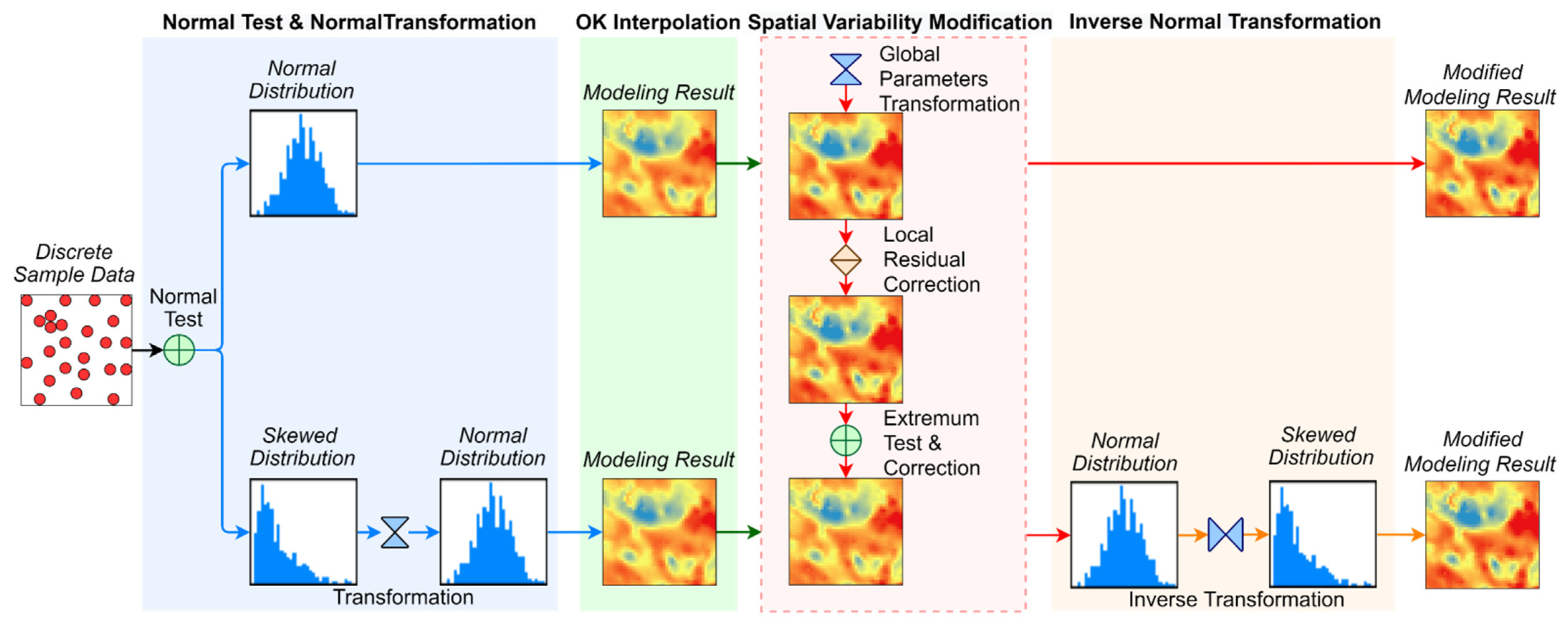
2. Spatial Variability Modified Ordinary Kriging Method (OK-SVM)

Since OK presents the problem of the underestimation of the spatial variability, we developed an OK post-processing method. In this method, the spatial variability of OK estimation is modified by cooperating with global parameters transformation, local residual correction, and extremum correction, so as to achieve high-precision reconstruction of the surface model of geographic objects with strong spatial variability from discrete sampling point datasets. The method contains a total of four computational processes, as shown in Figure 1.

2.1. Normal Test and Normal Transformation

Before performing ordinary kriging interpolation and spatial variability modification, the normality test of the data distribution should first be performed. Because the theoretical basis of kriging interpolation is to require sampled data to obey a normal distribution, it is thus more sensitive to outliers in skewed data. Moreover, the skewed data distribution used for modification of interpolation estimation may cause larger errors, so the data should be normally distributed as much as possible [36]. Therefore, the significantly skewed original sample point (SP) data should be normalized according to its distribution characteristics using the following transformation (Equation (1)).
Z ( x ) = F ( Z o   ( x ) )
where Z ( x ) is the transformed sample point data, Z o   ( x ) is the original sample point data, and F is the normal cumulative distribution function transformation.

2.2. Ordinary Kriging Interpolation

The second process is to calculate the value of each estimated point (EP) based on the SPs using OK interpolation. The value of each EP in OK interpolation is the sum of the linear weight of the measured value of all SPs in the given neighborhood (Equation (2)). Its calculation focuses on the solution of weight coefficients, and its estimated value needs to be unbiased and locally optimal. Therefore, OK interpolation must satisfy the condition that the mean value of the EPs is equal to that of the SPs, the sum of the weights is 1 (Equation (3)), and the least square method must be used to minimize the variance of the EPs (Equation (4)). According to the Lagrange multiplier method, Equation (4) can be further derived to obtain the OK interpolation equations (Equation (5)). By solving the (n + 1)-order linear equations, obtaining the kriging weight coefficients, and substituting it into Equation (2), the value of the EPs can be obtained.
Z ( x ) ^ = i = 1 n λ i Z ( x i )
i = 1 n λ i = 1
σ E 2 = c o v ¯ ( x 0 , x 0 ) + i = 1 n j = 1 n λ i λ j c o v ¯ ( x i , x j ) 2 i = 1 n c o v ¯ ( x 0 , x i )
{ j = 1 n λ j c o v ¯ ( x i , x j ) μ = c o v ¯ ( x 0 , x i ) j = 1 n λ j = 1  
In the Equations (2)–(5), Z ( x ) ^ is the value of the EPs, Z ( x i ) is the value of the SPs in the given range V ( i = 1 , 2 , 3 , n ) , λ i is the weight coefficient, σ E 2 is the variance of the EPs, and μ is the Lagrange multiplier.
Due to the least squares optimization method, the smaller values will be overestimated, and the larger values will be underestimated, which is the so-called “smoothing effect” [38,39]. The “smoothing effect” will also be intensified when the number of sample points in the estimation increases [39]. Moreover, this “smoothing effect” also shows non-uniformity in space, and the more distant the location from the SPs, the greater the “smoothing effect” will be [40].

2.3. Spatial Variability Modification

The reduction of the overall spatial variability after interpolation is essentially a deficit in global accuracy. The complex characteristics of geographic objects need to be reproduced by modifying the estimation results of spatial variability. However, the modification result often leads to a loss of local accuracy; that is, there is always a conflict between ensuring global spatial variability and local accuracy. This indicates that spatial variation modification is a nonlinear process. Therefore, a collaborative strategy of global parameters transformation, local residual correction, and extremum correction is proposed to achieve spatial variability modification without loss of local accuracy by coupling multiple linear processes.

2.3.1. Global Parameters Transformation (GPT)

The OK is an unbiased optimal estimate interpolator. However, in practice, cross-validation results show that the mean value of the EPs is almost equal to that of the SPs, and the variance of the EPs may be smaller than that of the SPs. This indicates that these two are two different sets with inconsistent global parameters (mean value and standard deviation). Therefore, in order to establish the modification relationship between them correctly, it is necessary to transform the two different sets into one set with uniform global parameters.
Z-score transformation (Equation (6)) is a commonly used data standardization method, which can transform two sets of data with different global parameters into a uniform standard score for comparing. Therefore, in the OK interpolation modification method proposed by Rezaee et al. [36] (OK-RM), the Z-score transformation is used for global parameters transformation of the EPs to improve its spatial variability, and the process is simple and easy to perform. This process is the same as OK-RM, which uses the Z-score transformation. The global parameters transformation based on Z-score consists of three steps. Firstly, the global parameters of the SPs and the EPs are calculated separately. Then, the Z-score transformation is performed on the EPs to obtain the standardized score (Equation (7)). Thirdly, the original global parameters of the EPs are replaced by those of the SPs, and then the inverse Z-score transformation is performed to obtain the new EPs (Equation (8)). After the aforementioned processing, the global parameters of the new EPs are consistent with those of the SPs. While ensuring unbiasedness, the spatial variability of the new EPs is significantly improved.
Z S c o r e = X E [ X ] V a r [ X ]
where Z S c o r e is the standard score after Z-score transformation, E [ X ] and V a r [ X ] are the mean value and standard deviation of the variable, respectively.
Z s ^ = Z ( x ) ^ E [ Z ( x ) ^ ] V a r [ Z ( x ) ^ ]
Z ( x ) ^ ^ = Z s ^ × V a r [ Z ( x ) ] + E [ Z ( x ) ]
In Equations (7) and (8), Z s ^ is the standard score of the EPs. Z ( x ) ^ ^ is the value after GPT of the EPs. E [ Z ( x ) ^ ] and E [ Z ( x ) ] are the mean values of the EPs and the SPs, respectively. V a r [ Z ( x ) ^ ] and V a r [ Z ( x ) ] are the standard deviations of the EPs and the SPs, respectively.

2.3.2. Local Residual Correction (LRC)

Since the foregoing process is essentially a global linear transformation, there is still a certain residual error in the spatial variability between the EPs and the SPs in the local neighborhood, which shows some impact on the reproduction of the spatial structure characteristics of regional variables. Therefore, differing from OK-RM, we need to make further corrections to the local residuals.
Firstly, the residuals on the SPs can be obtained from the measured value and the value after GPT (Equation (9)). Then, OK interpolation is performed again on the residuals at the SPs to estimate the residuals at all the EPs. Finally, the local residual correction results can be obtained by removing the residual part from the EPs’ value (Equation (10)). It should be noted here that since increasing the number of sample points involved in the estimation can intensify the “smoothing effect”, the interpolation of the residuals should be performed with a minimum number of local neighbor SPs to avoid the “smoothing effect” [35] on the residual estimation. The four SPs nearest to each EP in the local neighborhood are used in the calculation to avoid the “smoothing effect”.
R e E r r ( x s ) = Z ( x s ) ^ ^ Z ( x s )
Z ( x ) = Z ( x ) ^ ^ R e E r r ( x ) ^ ^
In the Equations (9) and (10), Z ( x s ) and Z ( x s ) ^ ^ are the measured value and the value after GPT on the SPs, R e E r r ( x s ) is the residual error on the SPs, R e E r r ( x ) ^ ^ is the estimated residual at the EPs, and Z ( x ) is the value after LRC of the EPS.

2.3.3. Extremum Test and Correction (ETC)

After the aforementioned LRC, it is possible that the values of the EPs fall outside the value range of their neighboring SPs. If so, the value after LRC of EPs also needs to be corrected. This is the other aspect that distinguishes it from OK-RM. It should be noted here that after the foregoing LRC, the global parameters of the EPs have changed. Therefore, differing from Yamamoto’s [35,41] extremum correction treatment, the above-mentioned transformation method needs to be used again to adjust the global parameters of the EPs in order to be able to compare with the SPs in its neighborhood. Then, by comparing with the maximum and minimum values of the SPs in the neighborhood (Equation (11)), the result after the ETC can be obtained (Equation (12)).
Δ = { Z ( x ) Z l _ m a x , Z ( x ) > Z l _ m a x Z ( x ) Z l _ m i n ,   Z ( x ) < Z l _ m i n
Z ( x ) ˜ = Z ( x ) Δ
In the Equations (11) and (12), Z ( x ) is the GPT result of the EPs after LRC, Z l _ m a x and Z l _ m i n are the extremum values of the SPs in the neighborhood, ∆ is the extremum difference between the EP and the SPs in the neighborhood, and Z ( x ) ˜   is the value after ETC of the EPs.
Similar to the previous process, if the global parameters of the EPs deviate significantly from those of the SPs after the ETC, the GPT of the EPs needs to be performed again to obtain the final correction result (Equation (13)).
Z ( x ) ˜ ˜ = ( Z ( x ) ˜ E [ Z ( x ) ˜ ] V a r [ Z ( x ) ˜ ] ) × V a r [ Z ( x ) ] + E [ Z ( x ) ]
where Z ( x ) ˜ ˜ is the final corrected value of the EPs and E [ Z ( x ) ˜ ] and V a r [ Z ( x ) ˜ ] are the mean value and standard deviation of the EPs after the ETC.

2.4. Inverse Normal Transformation

In most cases, the implementation objects are subjected to normal transformation to meet the application conditions of OK interpolation and Z-score transformation. Therefore, if the data are normalized before the modification, the result needs to be normalized inversely after the modification is completed to obtain the actual result (Equation (14)).
Z ( x ) ¯ ¯ = F 1 ( Z ( x ) ˜ ˜ )
where Z ( x ) ¯ ¯ is the modification result of the EPs after the inverse normal transformation and F 1 is the inverse normal transformation function.

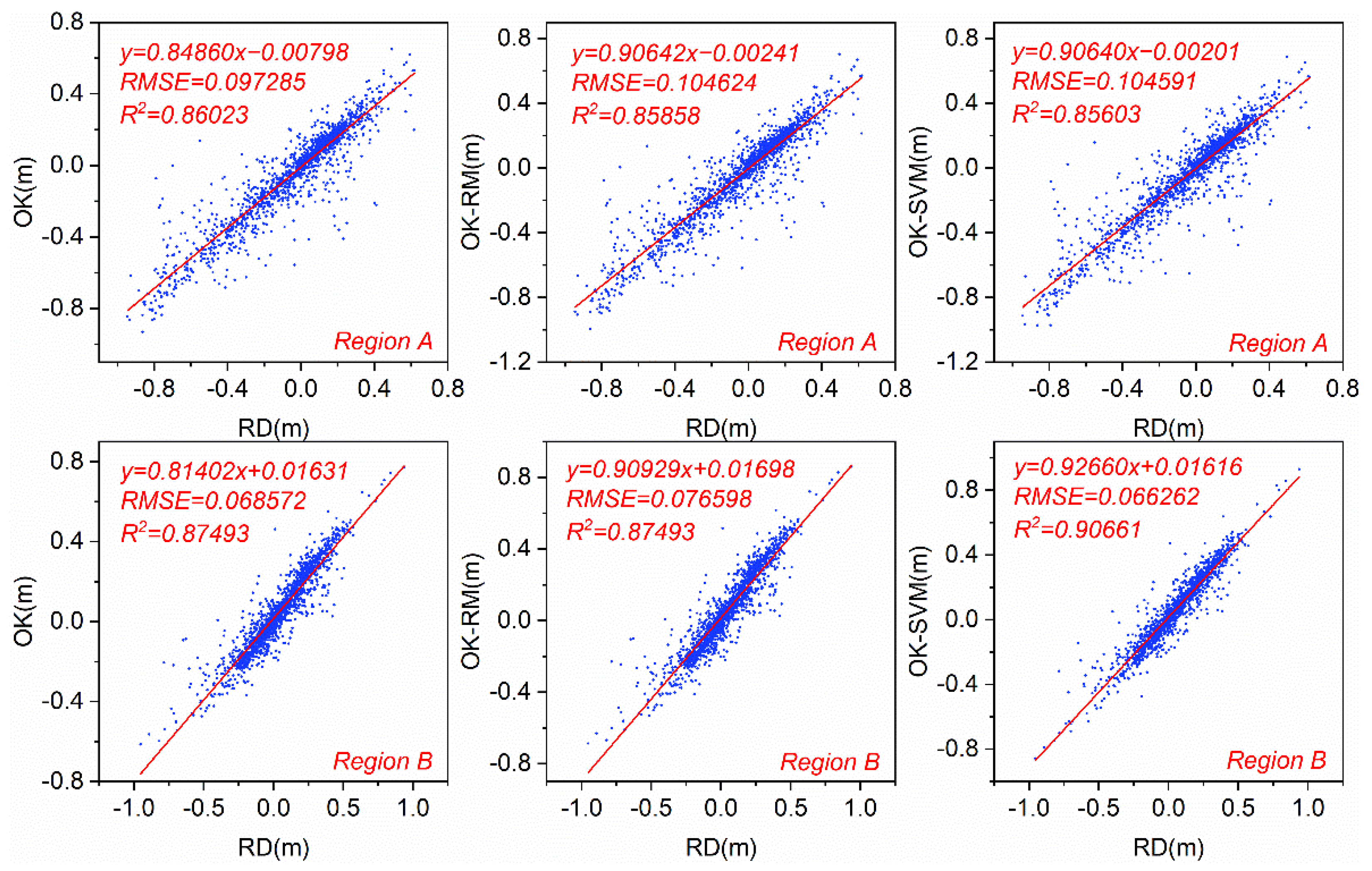
3. Robustness Test for Spatial Variability Modification

To test the robustness of the proposed modification method in the reproduction of spatial variability, we performed an experimental comparison analysis with OK and a simple OK post-processing method (OK-RM) [36].

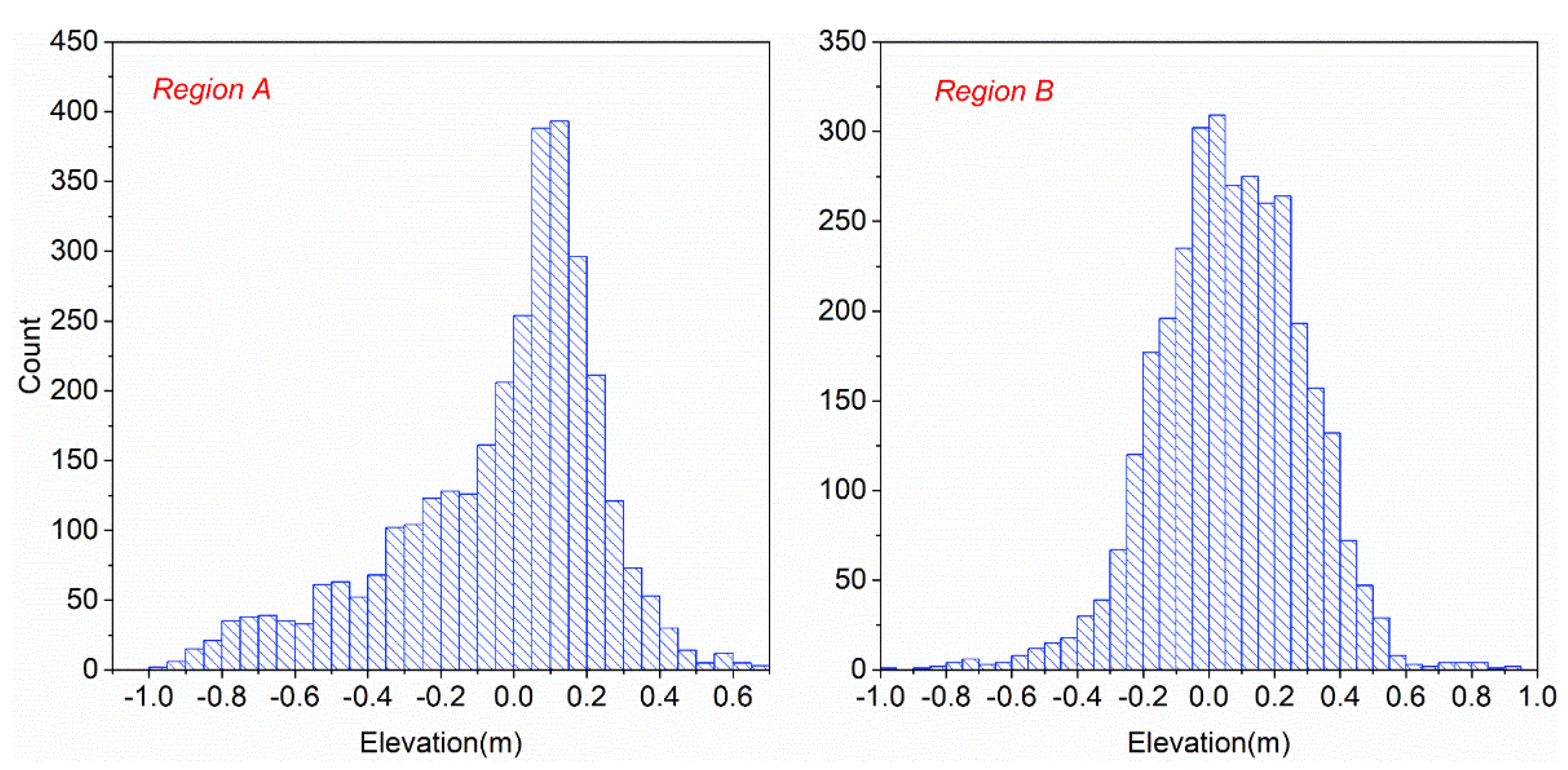
3.1. Experimental Data

Two regions with strong spatial variability (A and B) located on an island in China were selected as experimental objects. The raw data (RD) for them are both 52 × 63 raster format DEM (Figure 2) from the State Key Laboratory of Resources and Environmental Information System, Institute of Geographic Sciences and Natural Resources Research, Chinese Academy of Sciences (http://www.lreis.ac.cn/ (accessed on 30 October 2021)). Sample data (50%) and test data (the remaining 50%) were generated by random sampling from the RD for modeling estimation and verification. The data in region A showed skewed distribution and those in region B showed normal distribution, as shown in Figure 3.

3.2. Test Methods

Firstly, OK, OK-RM, and OK-SVM were used to reconstruct the two experimental objects based on sample points, respectively. Then, the structure difference of spatial variability between the estimated value and the true value at the test points was verified by semi-variogram reproduction. In addition, the residual means square error (RMSE), the slope, and the R-squared (R2) of the regression line between the estimated value and the true value were used to reflect the loss of local accuracy.

3.3. Test Results

The three methods use the same model parameter settings for comparison. The search neighborhood type is circular, with four sectors and 45° offset, the number of samples in the neighborhood is 10 points, and the semi-variogram fitting models are all spherical models. The reconstruction results are consistent with the spatial resolution of the TVs, as shown in Figure 4. The visual comparison shows that OK has an obvious “smoothing effect”. The value range of OK-RM is closer to the RD, although with a large difference in local features, so the results of OK-SVM are more consistent with the RD.
The reproduction results of the semi-variogram on the test point are shown in Figure 5. The semi-variogram of the estimated value of OK differs greatly from that of the true value, which also indicates that the “smoothing effect” causes a large error between the estimated value of OK and the true value in the spatial variation structure. The semi-variograms of OK-RM and OK-SVM are relatively close, but the results of OK-SVM are more consistent with the true value. This indicates that OK-SVM shows better performance in reflecting the real spatial variation structure characteristics of regional variables through spatial variability modification.
The local accuracy evaluation is shown in Figure 6. At the test points with skewed distribution, the results of OK-SVM are very close to OK-RM and OK in terms of R2, RMSE, and slope of the regression line. At the test points with normal distribution, the results of OK-SVM outperformed the other two methods. This shows that OK-SVM reduces the “smoothing effect” by modifying the spatial variability, while ensuring the local accuracy of the estimation results with strong robustness.

4. Case Study

4.1. Study Area and Datasets

The study area is located in a typical coral atoll (Figure 7b) in the Nansha Islands of the South China Sea (Figure 7a). An area covering about 15 km2 in the north of the region was selected as the study area (Figure 7b). The study area contains most of the geomorphic types of reef flat and lagoon (Figure 7c), including bio-clusters zone, reef pit zone, lagoon slope, lagoon bottom, and patch reef, with strong spatial variability.
The sampling points of geomorphology in the study area were obtained from the State Key Laboratory of Resources and Environmental Information System, Institute of Geographic Sciences and Natural Resources Research, Chinese Academy of Sciences (LREIS, IGSNRR, CAS). It was acquired by joint measurement of active remote sensing technology based on multi-beam and airborne lidar, with a total of 30,536,463 measurement points. The measured tidal data from the tide gauge stations in the study area were used for tide correction, and the outliers were checked and removed by manual editing. The corrected measurements were in the range of −25.65 m to 1.89 m.
To facilitate the subsequent evaluation of the accuracy and performance of the surface modeling methods, it is necessary to obtain a spatially continuous real geomorphological surface as the standard. However, both measurement sampling and modeling are generalizations of the real geomorphological surface, and it is impossible to obtain data that are completely consistent with the real geomorphological surface. Therefore, the real geomorphological surface is the logical object of expression and description, while the geomorphological generalization surface is the direct object of expression and description. The geomorphological generalization method is adopted here. First, the triangulated irregular network (TIN) surface model was constructed using all the measurement points. It was further converted into a grid DEM with a spatial resolution of 1 meter as the geomorphological generalization result (Figure 7d), which was used to replace the expression of the real geomorphological surface. Then, a random sampling method was used to extract 50% of the total measurement points for the reconstruction of the coral reef geomorphology. Finally, the reconstruction results and the generalization results were compared and analyzed to evaluate the geomorphological adaptability of different surface modeling methods.

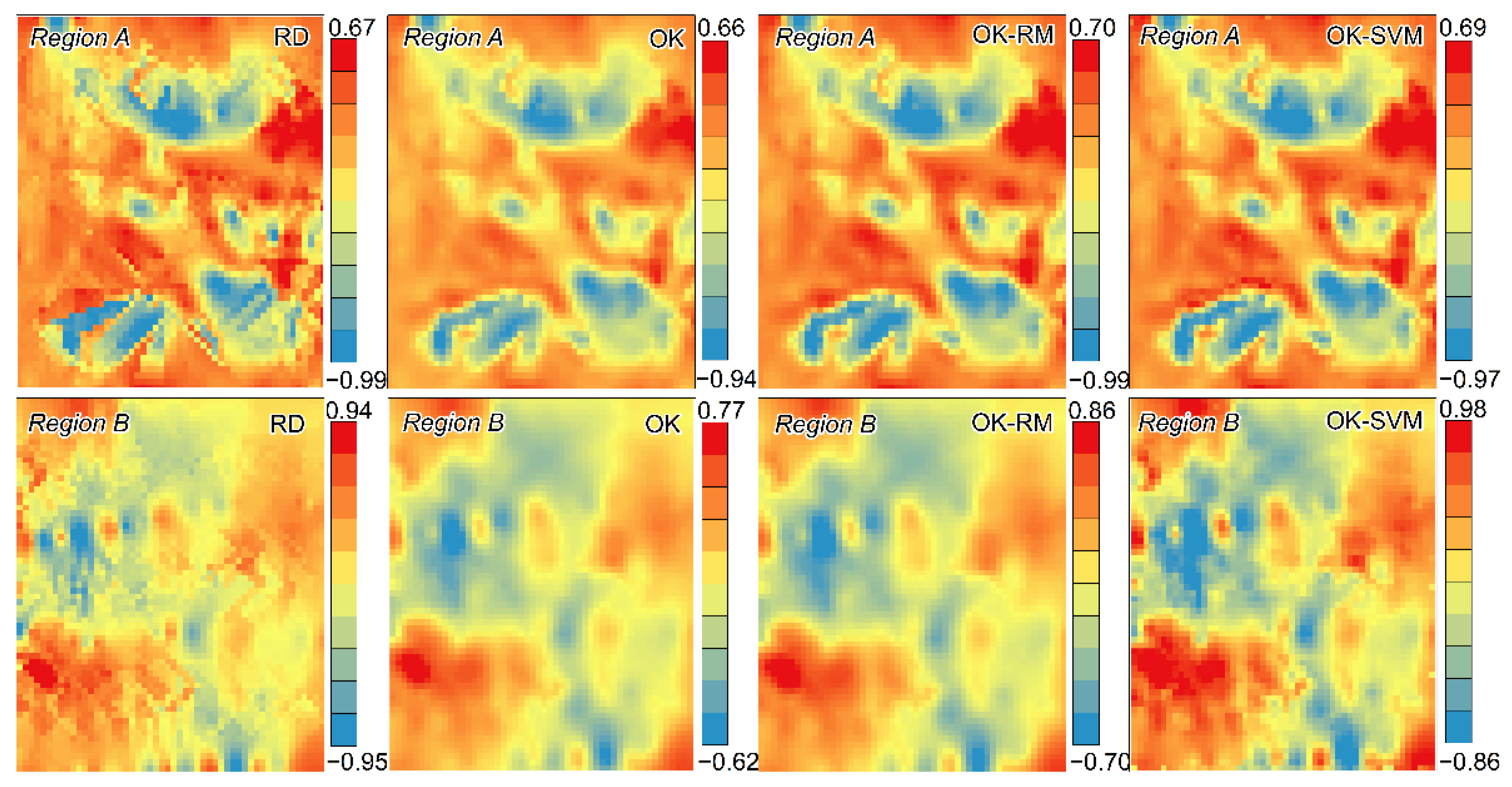
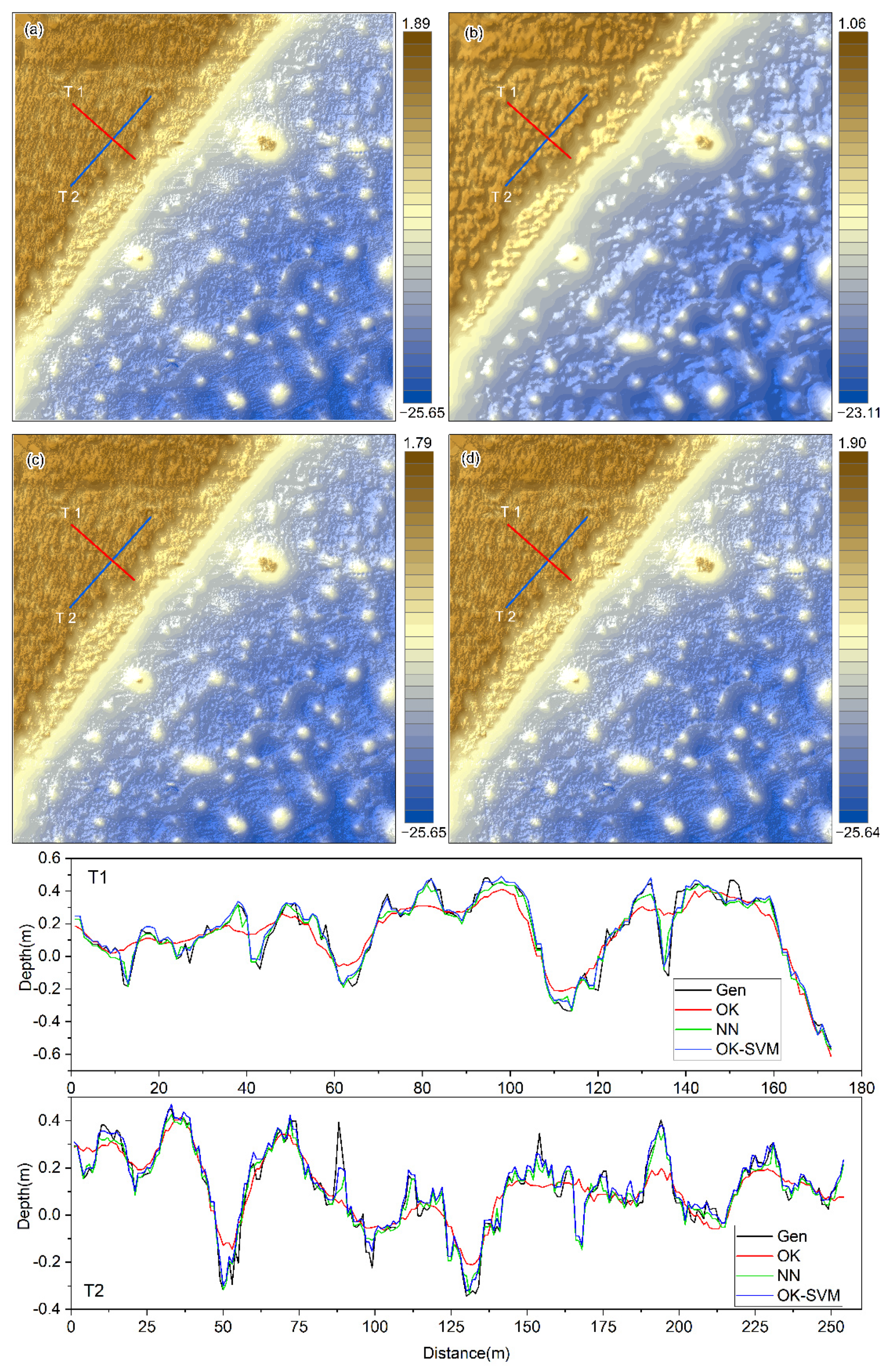
4.2. Reconstruction of Coral Reef Geomorphology

The geomorphological surface of the coral reef in the study area was reconstructed based on the OK-SVM method, with a spatial resolution of 1 m. Meanwhile, the OK and NN with excellent performance in the published research were selected for comparison. Among them, the model parameters of OK and OK-SVM are the same, the search neighborhood is circular, with four sectors and 45° offset, the neighborhood search radius is 10 points, and the semi-variogram fitting model is the spherical model. The reconstruction results of the above three methods are shown in Figure 8. The visual comparison results show that the geomorphological surface reconstructed by OK is quite different from the geomorphological generalization surface, while the results reconstructed by NN and OK-SVM are very close to the geomorphological generalization surface, and the expression of local details is finer than that of OK. From the perspective of the bottom depth range, OK-SVM is the closest to the geomorphological generalization surface, followed by NN and OK.

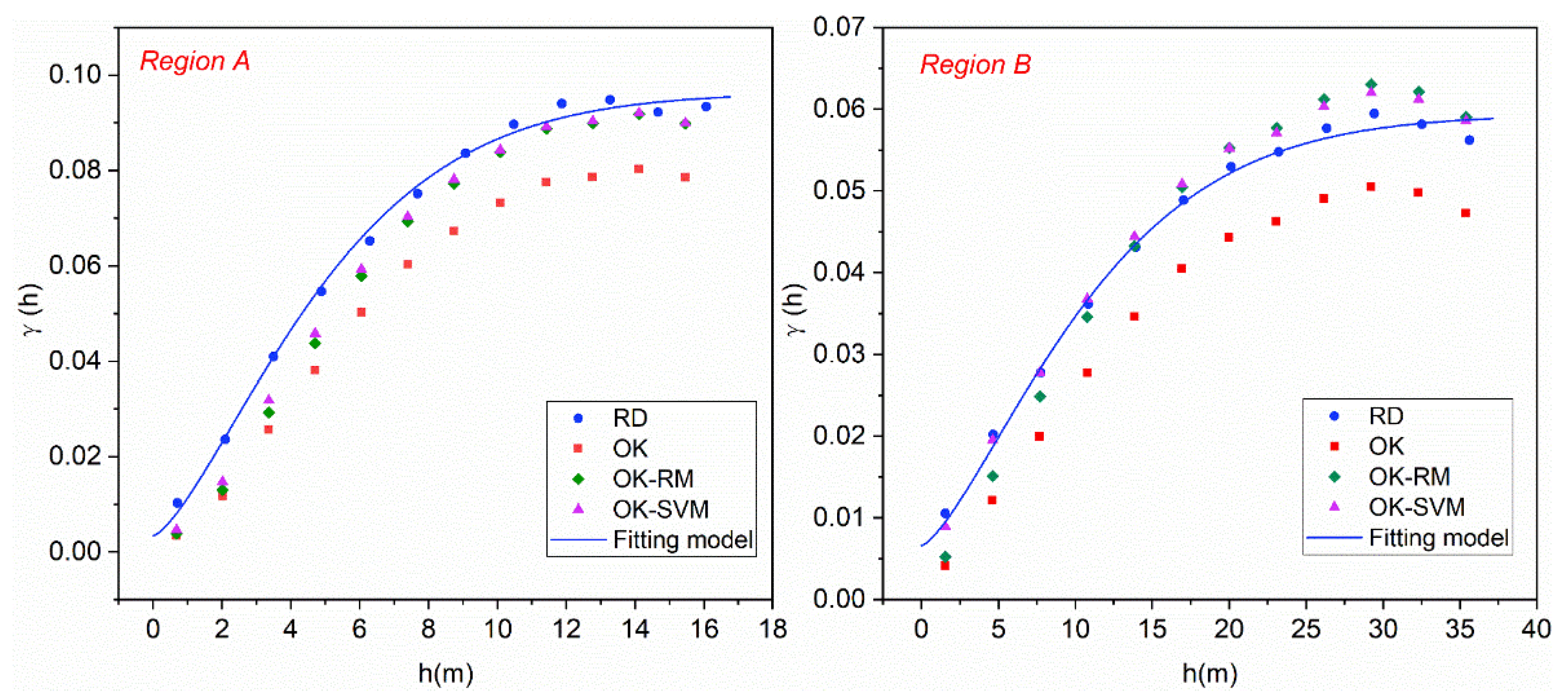
4.3. Comparative Analysis of Accuracy

Geomorphological reconstruction is often influenced by morphological distortion, which is mainly reflected in spatial relationships, geomorphic features, and local morphology. To evaluate the approximation degree between the reconstructed geomorphological surface and the geomorphological generalization surface from the perspective of morphological fidelity, we improved the evaluation index system for the geomorphological accuracy of coral reefs proposed by Wang et al. [42]. From the perspective of morphological fidelity of “point, line, and area“, an index system that considers morphological numerical accuracy (NA) and attribute accuracy (AA) is constructed (Table 1). The numerical accuracy indexes quantify the approximation degree of morphological features by numerical error, including the RMSE of local elevation (RMSE_LE), the RMSE of local aspect (RMSE_LA), and the RMSE of local relief (RMSE_LR). Attribute accuracy indexes quantify the change degree of morphological meaning by type attribute error, including the change rate of local elevation position (CR_LP), the change rate of local direction (CR_LD), and the change rate of local shape (CR_LS).
The numerical accuracy comparison (Figure 9) shows that the geomorphological surface reconstructed by OK-SVM is higher than OK in terms of local elevation, aspect, and convexity, and has a stronger correlation with the geomorphological generalization surface. Compared with the reconstruction results of NN, OK-SVM also has higher morphological numerical accuracy.
The comparison of attribute accuracy (Figure 10) shows that NN, OK, and OK-SVM have all changed 100% in terms of the attribute accuracy of the elevation location. This shows that no matter which method is used, it is difficult to reproduce the correct attributes of the elevation position. The shape attribute accuracy of OK-SVM is 39%, which is improved compared to NN (41%) and OK (47%). In terms of aspect attribute accuracy, OK-SVM (27%) is significantly higher than NN (75%) and OK (57%). This shows that the spatial variation modification has significantly improved the accuracy of the shape and aspect attributes of the reconstructed geomorphological surface. Comprehensive comparison can be drawn to show that OK-SVM has the highest morphological accuracy in the reconstruction of coral reef geomorphology, and its performance is better than NN and OK, and it can generate a geomorphological surface that is closer to reality.

5. Discussion

As with OK-RM, OK-SVM is also a post-processing method based on OK interpolation. Compared with OK and OK-RM, OK-SVM has an excellent performance in semi-variogram reproduction and local accuracy loss. This method shows high performance on both the reflection of the spatial variability structure characteristics and the local morphological characteristics, which provides a guarantee for the high-precision reconstruction of the coral reef geomorphology. It should be noted that the theoretical regression coefficient between the results after spatial variability modification and the true value should be equal to 1, while it is always close to 1 in practice. The main reason is that the method cannot completely modify its spatial variability to be consistent with the true one, and the results always have certain deviations [35]. The OK-RM proposed by Rezaee et al. [36] has made progress in terms of the simplicity of spatial variability modification compared with the classical post-processing method based on OK [35,41] due to the use of a global parameters transformation method based on Z-score. The OK-SVM proposed in this study also refers to the OK-RM in the spatial variability modification process, which can easily and conveniently improve the spatial variability of OK estimation. Compared with OK-RM, OK-SVM is more robust in spatial variability modification by coupling local residual correction and extremum correction processes, and the spatial variability is more consistent with reality without loss of local accuracy.
In cross-sectional comparison with OK and NN, which have excellent performance, the geomorphological surface reconstructed by OK-SVM is very close to the geomorphological generalization surface of coral reef, and it shows higher morphological numerical accuracy. A longitudinal comparison of the numerical accuracy indexes shows that the correlation between the reconstructed geomorphological surfaces and the geomorphological generalization surface in terms of LR is the lowest for NN, OK, or OK-SVM. The main reason is that the LR, the accuracy indicator of the “area” feature, is affected by the “smoothing effect” deeper than the other two numerical accuracy indicators. However, OK-SVM has relatively less accuracy loss in LR. In addition, OK-SVM has a relatively lower change ratio of morphological attributes. This is very critical, because morphological attributes are usually important parameters for the quantification and evolution of coral reef geomorphology [43,44]. Therefore, the collaborative spatial variability modification strategy of global parameters transformation, local residual correction, and extremum correction makes OK-SVM more adaptable in the geomorphological reconstruction of coral reefs with strong spatial variability. This will provide a guarantee for the subsequent accurate calculation of the multi-scale coral reef geomorphological parameters, which is beneficial to the research of active and passive remote sensing cooperative classification of coral reef geomorphology and analysis of coral reef ecological changes.
OK-SVM is a multi-process coupling method and contains two OK calculations, which will undoubtedly reduce the efficiency of the calculation for large data volume. Therefore, high-performance computing devices can be approached to solve this problem in large data volume computing scenarios. In addition, we need to conduct further research in the following aspects. In terms of the adaptability of high-precision coral reef geomorphological reconstruction, the OK and NN, which have been tested in the field of geomorphological reconstruction of coral reefs, were chosen for comparison. We will compare the adaptability of the proposed method with other methods for coral reef geomorphological reconstruction applications in our future research work. Because of the scale effect of interpolation on the representation of geographic phenomena [45,46], the reduction of spatial resolution will affect the accuracy of spatial variability representation. In this study, a high spatial resolution scale was selected for analysis, in order to lay the foundation for co-interpretation with high-resolution passive remote sensing datasets. Our next step will be to conduct related research in the selection of suitable scales. The lack of measurement data in some areas during coral reef geomorphology monitoring is a practical problem and one that cannot be ignored. Thus, the performance of the method in dealing with such cases needs to be tested in future work. Moreover, it is important to note that the OK-SVM proposed here has the potential to be applied to other surface modeling studies with strong spatial variability characteristics. Therefore, we will also test its performance in other potential modeling application areas in future research work.

6. Conclusions

Reconstruction of spatially continuous and high-precision coral reef geomorphological surfaces based on active remote sensing datasets is the basis for achieving accurate extraction of coral reef geomorphological parameters, which is crucial for coral reef geomorphological and ecological change studies. Surface modeling methods such as OK and NN, which have been frequently used in existing studies, have the problem of low estimation of spatial variability in the application of coral reef geomorphological reconstruction. This can have an impact on the accurate calculation of coral reef geomorphological parameters. To address the problem, an OK-SVM method is proposed in this study. This method adopts a collaborative strategy of global parameters transformation, local residual correction, and extremum correction to modify the underestimated spatial variability of the reconstructed surfaces, while avoiding the loss of local accuracy. The experimental results show that OK-SVM is highly robust in spatial variability modification. Meanwhile, the results of the application case study of coral reef geomorphological reconstruction show that, compared with OK and NN, the OK-SVM performs better in terms of detailed morphological fidelity, the reconstructed surface has higher morphological accuracy, and is more adaptable in the reconstruction of coral reef geomorphology with strong spatial variability.
This method can be used as a reliable tool for reconstructing high-precision coral reef complex geomorphology from active remote sensing data, compared with the commonly used methods in this field. Other potential modeling application areas of the proposed method will also be tested in the future.

Author Contributions

Conceptualization, Q.W. and F.S.; methodology, Q.W. and H.X.; validation, H.X. and Q.W.; resources, F.S.; data curation, F.S.; writing—original draft preparation, Q.W.; writing—review and editing, H.X., W.W. and X.Z.; visualization, X.Z. and Q.W.; supervision, F.S.; project administration, F.S., Q.W., G.Y. and G.Z.; funding acquisition, F.S., Q.W., G.Y. and G.Z. All authors have read and agreed to the published version of the manuscript.

Funding

This research was funded by “Key Program of Frontier Science of Chinese Academy of Sciences, grant number QYZDY-SSW-DQC019”, “Ph.D. Programs Foundation of Shandong Jianzhu University, grant number XNBS1984”, “National Natural Science Foundation of China, grant number 42171435”, and “Shandong Provincial Natural Science Foundation, grant number ZR2021DQ021”.

Data Availability Statement

Not applicable.

Acknowledgments

The authors are grateful to the State Key Laboratory of Resources and Environmental Information System (SKLREIS), Institute of Geographic Sciences and Natural Resources Research, Chinese Academy of Sciences (IGSNRR, CAS) for providing the active remote sensing datasets.

Conflicts of Interest

The authors declare no conflict of interest.

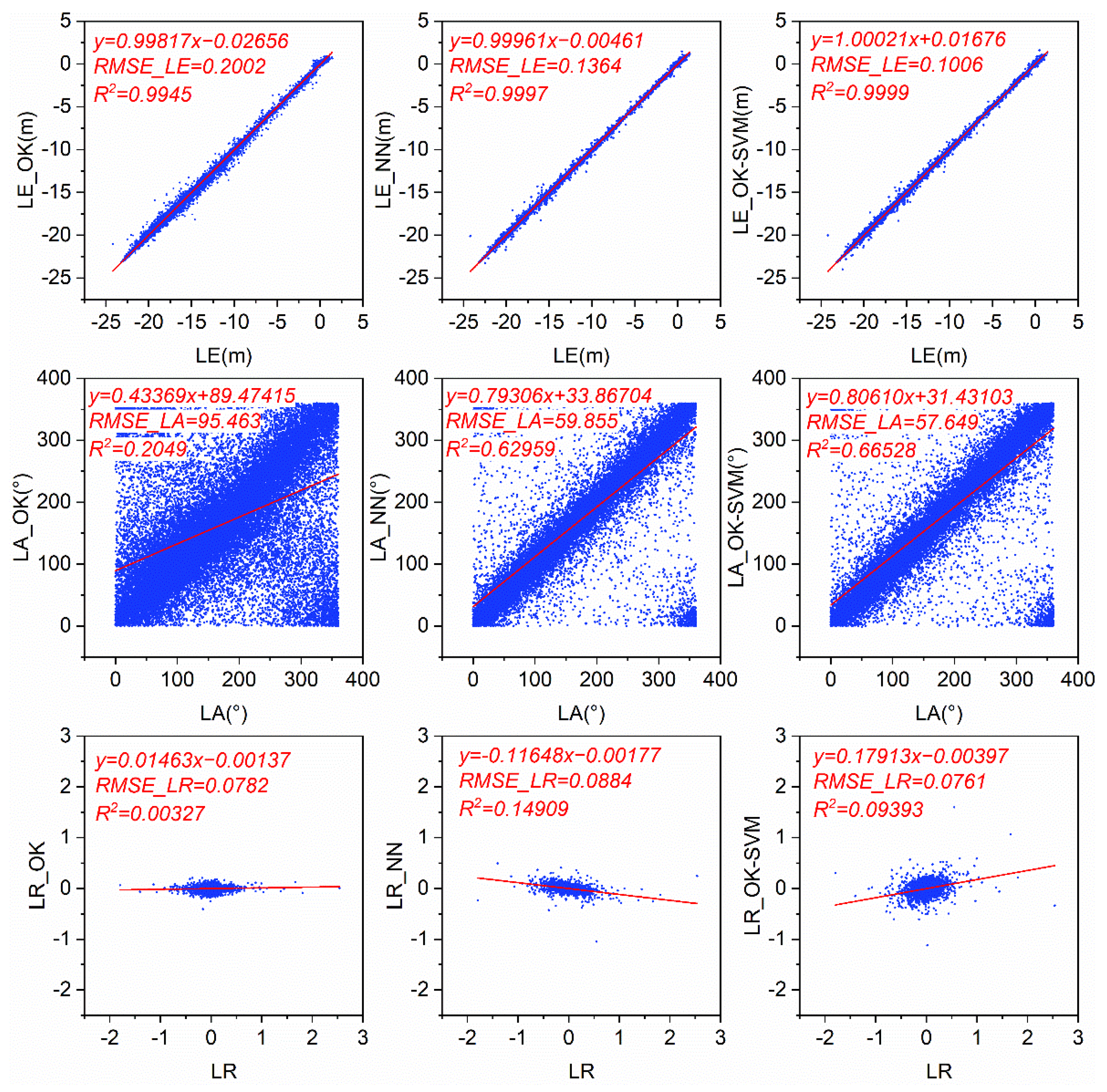
Appendix A. Calculation Processes of Morphological Fidelity Evaluation Index System

Appendix A.1. Analysis Scale

The accuracy evaluation scale is defined as a 3 × 3 local neighborhood (Figure A1), which is used as the smallest unit for geomorphological fidelity analysis. The evaluation indexes are calculated from the values of the central pixel and its eight neighboring pixels.
Figure A1. Analysis scale.
Remotesensing 14 00253 g0a1

Appendix A.2. Calculation Process

Appendix A.2.1. RMSE of Local Elevation (RMSE_LE)

(1)
Use test points to extract the elevation values of the reconstructed geomorphological surface and the geomorphological generalization surface, respectively, and calculate the errors between them.
(2)
Calculate the root mean square error of elevation error at all test points.

Appendix A.2.2. RMSE of Local Aspect (RMSE_LA)

(1)
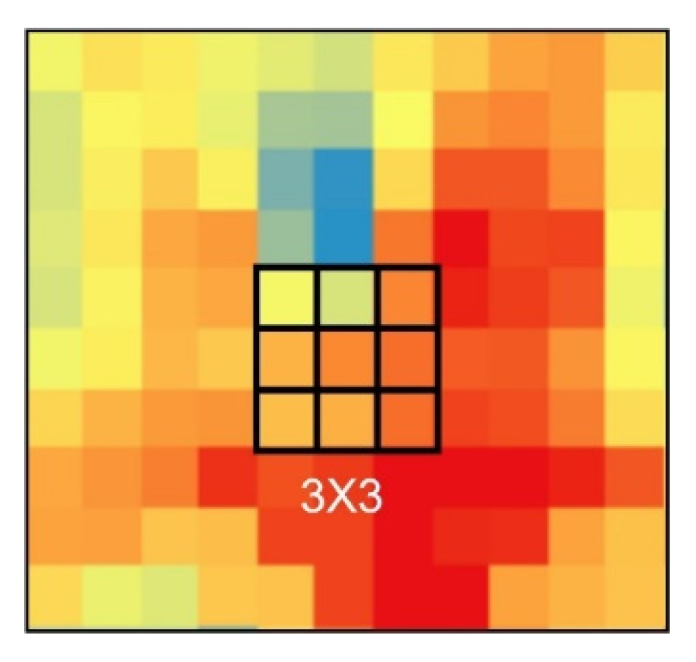
Calculate the aspect of the reconstructed geomorphological surface and the geomorphological generalization surface using a 3 × 3 neighborhood window, respectively.
(2)
Use the test points to extract their aspect values in the reconstructed geomorphological surface and the geomorphological generalization surface, respectively, and calculate the error between them.
(3)
Calculate the root mean square error of the aspect error on all test points.

Appendix A.2.3. RMSE of Local Relief (RMSE_LR)

(1)
Calculate the mean values of the reconstructed geomorphological surface and the geomorphological generalization surface using a 3 × 3 neighborhood window, respectively.
(2)
Calculate the local relief of each position by subtracting the mean values from the reconstructed geomorphological surface and the geomorphological generalization surface, respectively.
(3)
Use the test points to extract their local relief values in the reconstructed geomorphological surface and the geomorphological generalization surface, respectively, and calculate the error between them.
(4)
Calculate the root mean square error of the local relief error on all test points.

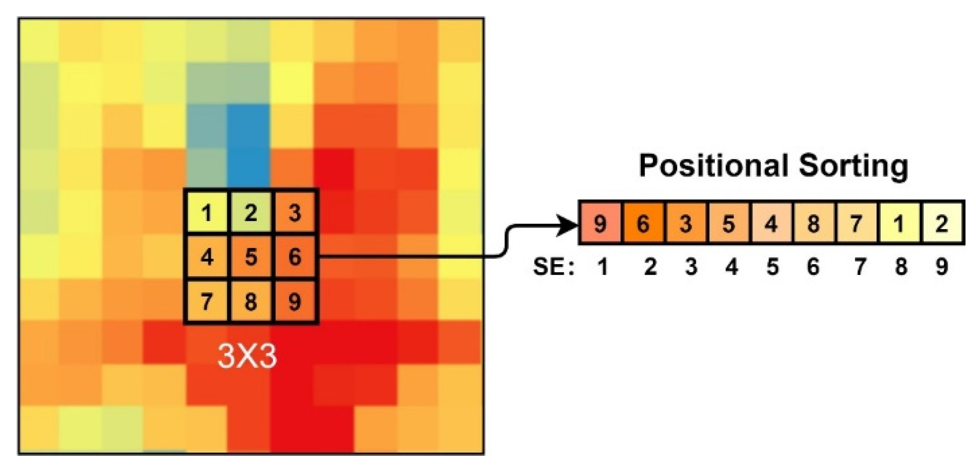
Appendix A.2.4. Change Rate of Local Elevation Position (CR_LP)

(1)
Sort the elevation values of local neighborhoods in the reconstructed morphological surface to obtain position relations, as shown in Figure A2. The position relations of the test points in the geomorphological generalization surface are obtained by the same method.
(2)
Comparing the results of the two, if they are different, it is considered that the elevation position relationships of the test points have changed.
(3)
Obtain the CR_LP by calculating the number of the test points whose elevation position relationship changed among all test points.
Figure A2. Calculation of elevation position relationship.
Remotesensing 14 00253 g0a2

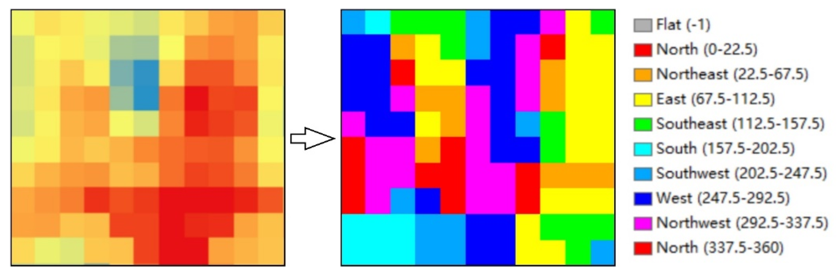
Appendix A.2.5. Change Rate of Local Direction (CR_LD)

(1)
Reclassify the local aspect values of the reconstructed morphological surface and the geomorphological generalization surface into directions, as shown in Figure A3.
(2)
Use the test points to extract their local directions in the reconstructed geomorphological surface and the geomorphological generalization surface, respectively.
(3)
Obtain the CR_LD by calculating the number of test points whose local directions changed among all test points.
Figure A3. Aspect reclassification.
Remotesensing 14 00253 g0a3

Appendix A.2.6. Change Rate of Local Shape (CR_LS)

(1)
Reclassify the local relief values of the reconstructed geomorphological surface and the geomorphological generalization surface. Those greater than 0 are concave, those less than 0 are convex, and those equal to 0 are flat.
(2)
Use the test points to extract their local convexity attributes in the reconstructed geomorphological surface and the geomorphological generalization surface, respectively.
(3)
Obtain the CR_LS by calculating the number of test points whose local convexity changed among all test points.

References

  1. Kayanne, H.; Aoki, K.; Suzuki, T.; Hongo, C.; Yamano, H.; Ide, Y.; Iwatsuka, Y.; Takahashi, K.; Katayama, H.; Sekimoto, T.; et al. Eco-geomorphic processes that maintain a small coral reef island: Ballast Island in the Ryukyu Islands, Japan. Geomorphology 2016, 271, 84–93. [Google Scholar] [CrossRef]
  2. Coles, S.L.; Looker, E.; Burt, J.A. Twenty-year changes in coral near Muscat, Oman estimated from manta board tow observations. Mar. Environ. Res. 2015, 103, 66–73. [Google Scholar] [CrossRef]
  3. Perry, C.T.; Smithers, S.G.; Kench, P.S.; Pears, B. Impacts of Cyclone Yasi on nearshore, terrigenous sediment-dominated reefs of the central Great Barrier Reef, Australia. Geomorphology 2014, 222, 92–105. [Google Scholar] [CrossRef] [Green Version]
  4. Hughes, T.P.; Huang, H.; Young, M.A.L. The Wicked Problem of China’s Disappearing Coral Reefs. Conserv. Biol. 2013, 27, 261. [Google Scholar] [CrossRef]
  5. Lapointe, B.E.; Thacker, K.; Hanson, C.; Getten, L. Sewage pollution in Negril, Jamaica: Effects on nutrition and ecology of coral reef macroalgae. Chin. J. Oceanol. Limnol. 2011, 29, 775–789. [Google Scholar] [CrossRef]
  6. Mcwilliams, J.P.; Côté, I.M.; Gill, J.A.; Sutherland, W.J.; Watkinson, A.R. Accelerating impacts of temperature-induced coral bleaching in the Caribbean. Ecology 2005, 86, 2055–2060. [Google Scholar] [CrossRef] [Green Version]
  7. Liu, G.; Strong, A.E.; Skirving, W. Remote sensing of sea surface temperatures during 2002 Barrier Reef coral bleaching. Eos Trans. Am. Geophys. Union 2003, 84, 137–141. [Google Scholar] [CrossRef]
  8. Wilkinson, C. Status of Coral Reefs of the World: 2008; Global Coral Reef Monitoring Network and Reef and Rainforest Research Centre: Townsville, Australia, 2008; p. 296. [Google Scholar]
  9. Palandro, D.A.; Andréfouët, S.; Hu, C.; Hallock, P.; Müller-Karger, F.E.; Dustan, P.; Callahan, M.K.; Kranenburg, C.; Beaver, C.R. Quantification of two decades of shallow-water coral reef habitat decline in the Florida Keys National Marine Sanctuary using Landsat data (1984–2002). Remote Sens. Environ. 2008, 112, 3388–3399. [Google Scholar] [CrossRef]
  10. Rogers, C.; Miller, J. Permanent ‘phase shifts’ or reversible declines in coral cover? Lack of recovery of two coral reefs inSt. John, US Virgin Islands. Mar. Ecol. Prog. 2006, 306, 103–114. [Google Scholar] [CrossRef]
  11. Hoegh-Guldberg, O. Climate change, coral bleaching and the future of the world’s coral reefs. Mar. Freshw. Res. 1999, 50, 839–866. [Google Scholar] [CrossRef] [Green Version]
  12. Araújo, P.; Amaral, R.F. Mapping of coral reefs in the continental shelf of Brazilian Northeast through remote sensing. Rev. Gestão Costeira Integr. 2016, 16, 5–20. [Google Scholar] [CrossRef] [Green Version]
  13. Xu, J.; Zhao, D. Review of coral reef ecosystem remote sensing. Acta Ecol. Sin. 2014, 34, 19–25. [Google Scholar] [CrossRef]
  14. Dubinsky, Z.; Stambler, N. Coral Reefs: An Ecosystem in Transition; Springer: Dordrecht, The Netherlands, 2011. [Google Scholar]
  15. Scopélitis, J.; Andréfouët, S.; Phinn, S.; Arroyo, L.; Dalleau, M.; Cros, A.; Chabanet, P. The next step in shallow coral reef monitoring: Combining remote sensing and in situ approaches. Mar. Pollut. Bull. 2010, 60, 1956–1968. [Google Scholar] [CrossRef]
  16. Mumby, P.J.; Skirving, W.; Strong, A.E.; Hardy, J.T.; LeDrew, E.F.; Hochberg, E.J.; Stumpf, R.P.; David, L.T. Remote sensing of coral reefs and their physical environment. Mar. Pollut. Bull. 2004, 48, 219–228. [Google Scholar] [CrossRef] [PubMed]
  17. Xu, J.; Zhao, J.; Li, F.; Wang, L.; Song, D.; Wen, S.; Wang, F.; Gao, N. Object-based image analysis for mapping geomorphic zones of coral reefs in the Xisha Islands, China. Acta Oceanol. Sin. 2016, 35, 19–27. [Google Scholar] [CrossRef]
  18. Lucas, M.Q.; Goodman, J. Linking Coral Reef Remote Sensing and Field Ecology: It’s a Matter of Scale. J. Mar. Sci. Eng. 2015, 3, 1–20. [Google Scholar] [CrossRef]
  19. Marchese, F.; Bracchi, V.A.; Lisi, G.; Basso, D.; Corselli, C.; Savini, A. Assessing Fine-Scale Distribution and Volume of Mediterranean Algal Reefs through Terrain Analysis of Multibeam Bathymetric Data. A Case Study in the Southern Adriatic Continental Shelf. Water 2020, 12, 157. [Google Scholar] [CrossRef] [Green Version]
  20. Su, D.P.; Yang, F.L.; Ma, Y.; Zhang, K.; Huang, J.; Wang, M.W. Classification of Coral Reefs in the South China Sea by Combining Airborne LiDAR Bathymetry Bottom Waveforms and Bathymetric Features. IEEE Trans. Geosci. Remote Sens. 2019, 57, 815–828. [Google Scholar] [CrossRef]
  21. Zhang, K.; Yang, F.; Zhang, H.; Su, D.; Li, Q.Q. Morphological characterization of coral reefs by combining LiDAR and MBES data: A case study from Yuanzhi Island, South China Sea. J. Geophys. Res. Ocean. 2017, 122, 4779–4790. [Google Scholar] [CrossRef]
  22. Leon, J.; Woodroffe, C. The use of digital terrain models in coral reef geomorphology. In Proceedings of the 8th International Symposium on GIS and Computer Mapping for Coastal Zone Management, Santander, Spain, 8–10 October 2007; pp. 454–463. [Google Scholar]
  23. Anelli, M.; Julitta, T.; Fallati, L.; Galli, P.; Rossini, M.; Colombo, R. Towards new applications of underwater photogrammetry for investigating coral reef morphology and habitat complexity in the Myeik Archipelago, Myanmar. Geocarto Int. 2019, 34, 459–472. [Google Scholar] [CrossRef]
  24. Zawada, D.G.; Brock, J.C. A Multiscale Analysis of Coral Reef Topographic Complexity Using Lidar-Derived Bathymetry. J. Coast. Res. 2009, 25, 6–15. [Google Scholar] [CrossRef]
  25. Walker, B.K.; Jordan, L.; Spieler, R.E. Relationship of Reef Fish Assemblages and Topographic Complexity on Southeastern Florida Coral Reef Habitats. J. Coast. Res. 2009, 53, 39–48. [Google Scholar] [CrossRef]
  26. Costa, B.M.; Battista, T.A.; Pittman, S.J. Comparative evaluation of airborne LiDAR and ship-based multibeam SoNAR bathymetry and intensity for mapping coral reef ecosystems. Remote Sens. Environ. 2009, 113, 1082–1100. [Google Scholar] [CrossRef]
  27. Zarco-Perello, S.; Simoes, N. Ordinary kriging vs inverse distance weighting: Spatial interpolation of the sessile community of Madagascar reef, Gulf of Mexico. PEERJ 2017, 5, e4078. [Google Scholar] [CrossRef] [Green Version]
  28. Coleman, J.B.; Yao, X.; Jordan, T.R.; Madden, M. Holes in the ocean: Filling voids in bathymetric lidar data. Comput. Geosci. 2011, 37, 474–484. [Google Scholar] [CrossRef]
  29. Ding, Q.; Wang, Y.; Zhuang, D. Comparison of the common spatial interpolation methods used to analyze potentially toxic elements surrounding mining regions. J. Environ. Manag. 2018, 212, 23–31. [Google Scholar] [CrossRef] [PubMed]
  30. Desmet, P.J.J. Effects of Interpolation Errors on the Analysis of DEMs. Earth Surf. Processes Landf. 2015, 22, 563–580. [Google Scholar] [CrossRef]
  31. Arun, P.V. A comparative analysis of different DEM interpolation methods. Egypt. J. Remote Sens. Space Sci. 2013, 16, 133–139. [Google Scholar] [CrossRef] [Green Version]
  32. Wedding, L.M.; Friedlander, A.M.; McGranaghan, M.; Yost, R.S.; Monaco, M.E. Using bathymetric lidar to define nearshore benthic habitat complexity: Implications for management of reef fish assemblages in Hawaii. Remote Sens. Environ. 2008, 112, 4159–4165. [Google Scholar] [CrossRef]
  33. Conger, C.L.; Fletcher, C.H.; Hochberg, E.H.; Frazer, N.; Rooney, J.J.B. Remote sensing of sand distribution patterns across an insular shelf: Oahu, Hawaii. Mar. Geol. 2009, 267, 175–190. [Google Scholar] [CrossRef]
  34. Leon, J.X.; Phinn, S.R.; Hamylton, S.; Saunders, M.I. Filling the ‘white ribbon’—A multisource seamless digital elevation model for Lizard Island, northern Great Barrier Reef. Int. J. Remote Sens. 2013, 34, 6337–6354. [Google Scholar] [CrossRef]
  35. Yamamoto, J.K. Correcting the Smoothing Effect of Ordinary Kriging Estimates. Math. Geol. 2005, 37, 69–94. [Google Scholar] [CrossRef]
  36. Rezaee, H.; Asghari, O.; Yamamoto, J.K. On the reduction of the ordinary kriging smoothing effect. J. Min. Environ. 2011, 2, 102–117. [Google Scholar] [CrossRef]
  37. Chen, C.; Liu, F.; Li, Y.; Yan, C.; Liu, G. A robust interpolation method for constructing digital elevation models from remote sensing data. Geomorphology 2016, 268, 275–287. [Google Scholar] [CrossRef]
  38. Goovaerts, P. Geostatistics for Natural Resource Evaluation; Oxford University Press: Oxford, UK, 1997. [Google Scholar]
  39. Isaaks, E.H.; Srivastava, M.R. An Introduction to Applied Geostatistics; Oxford University Press: New York, NY, USA, 1989. [Google Scholar]
  40. Journel, A.G.; Kyriakidis, P.C.; Mao, S. Correcting the Smoothing Effect of Estimators: A Spectral Postprocessor. Math. Geol. 2000, 32, 787–813. [Google Scholar] [CrossRef]
  41. Yamamoto, J.K. On unbiased backtransform of lognormal kriging estimates. Comput. Geosci. 2007, 11, 219–234. [Google Scholar] [CrossRef]
  42. Wang, Q.; Su, F.; Zhang, Y.; Jiang, H.; Cheng, F. Morphological Precision Assessment of Reconstructed Surface Models for a Coral Atoll Lagoon. Sustainability 2018, 10, 2749. [Google Scholar] [CrossRef] [Green Version]
  43. Duce, S.; Vila-Concejo, A.; Hamylton, S.M.; Webster, J.M.; Bruce, E.; Beaman, R.J. A morphometric assessment and classification of coral reef spur and groove morphology. Geomorphology 2016, 265, 68–83. [Google Scholar] [CrossRef]
  44. Zieger, S.; Stieglitz, T.; Kininmonth, S. Mapping reef features from multibeam sonar data using multiscale morphometric analysis. Mar. Geol. 2009, 264, 209–217. [Google Scholar] [CrossRef]
  45. Drăguţ, L.; Eisank, C. Object representations at multiple scales from digital elevation models. Geomorphology 2011, 129, 183–189. [Google Scholar] [CrossRef] [Green Version]
  46. Smith, M.P.; Zhu, A.X.; Burt, J.E.; Stiles, C. The effects of DEM resolution and neighborhood size on digital soil survey. Geoderma 2006, 137, 58–69. [Google Scholar] [CrossRef]
Figure 1. Schematic diagram of processing steps. The blue panel is the first step, which is to test the normality of the discrete sample data, and to perform the normal transformation if the sample data distribution has non-normality. The green panel is the second step, which is to construct a spatially continuous surface model by OK interpolation. The pink panel is the third step, which is to modify the spatial variability of the surface model by global parameters transformation and local residual correction. The orange panel is the fourth step, which is to carry out the inverse normal transformation for the processing results of normal transformation to obtain the original scale.
Remotesensing 14 00253 g001
Figure 2. Experimental data: the left is the RD, the middle is the sample points (SPs), and the right is the test points (TPs).
Remotesensing 14 00253 g002
Figure 3. Histogram of experimental data: region A presents a skewed distribution and region B presents a normal distribution.
Remotesensing 14 00253 g003
Figure 4. Comparison of reconstruction results: from left to right are the RD, OK estimation, OK-RM estimation, and OK-SVM estimation, respectively.
Remotesensing 14 00253 g004
Figure 5. Semi-variogram reproduction: the blue dots are the spatial variation structure of the truth value, the red squares are the spatial variation structure of the OK estimation, the green diamonds are the spatial variation structure of the OK-RM estimation, the purple triangles are the spatial variation structure of the OK-SVM estimation, and the blue curves are the fitting models.
Remotesensing 14 00253 g005
Figure 6. Local accuracy evaluation: from left to right are the local accuracy evaluation results of the OK estimation, OK-RM estimation, and OK-SVM estimation, respectively.
Remotesensing 14 00253 g006
Figure 7. Study area: (a) is the geographical location of the study object; (b) is the high-resolution image of the study object, where the red rectangle is the research area; (c) is the geomorphic classification of the study object; (d) is the geomorphological generalization of the study area.
Remotesensing 14 00253 g007
Figure 8. Comparison of reconstructed coral reef geomorphology: (a) geomorphological generalization surface, (b) geomorphological surface reconstructed by OK, (c) geomorphological surface reconstructed by NN, (d) geomorphological surface reconstructed by OK-SVM. T1 and T2 are two intersecting transect lines; the black lines are transects of the geomorphological generalization surface, the red lines are transects of the geomorphological surface reconstructed by OK, the green lines are transects of the geomorphological surface reconstructed by NN, and the blue lines are transects of the geomorphological surface reconstructed by OK-SVM.
Remotesensing 14 00253 g008
Figure 9. Numerical accuracy comparison of reconstructed coral reef geomorphology: from left to right are the numerical accuracy of OK, NN, and OK-SVM.
Remotesensing 14 00253 g009
Figure 10. Attribute accuracy comparison of reconstructed coral reef geomorphology: the orange is the attribute accuracy of OK, the green is the attribute accuracy of NN, and the purple is the attribute accuracy of OK-SVM.
Remotesensing 14 00253 g010
Table 1. Morphological fidelity evaluation index system (the calculation processes are provided in Appendix A).
CategoryIndexesDescription and Morphological Meanings
NA R M S E _ L E = 1 n i = 1 n ( Z * Z ) 2 Where   Z * ,   A * ,   R * are the local elevation (LE), local aspect (LA), and local relief (LR) of reconstructed surface at the test points, respectively, and Z, A, R   are   those   of   generalization   surface   at   the   test   points ,   respectively .   The   smaller   R M S E _ L E ,   R M S E _ L A ,   and   R M S E _ L R are, the closer the reconstructed surface is to the generalization surface, and the higher the morphological numerical accuracy is.
R M S E _ L A = 1 n i = 1 n ( A * A ) 2
R M S E _ L R = 1 n i = 1 n ( R * R ) 2
AA C R _ L P = N L P N Where N   is   the   number   of   the   test   points   and   N L P ,   N L D ,   N L S   are   the   changes   numbers   in   the   local   elevation   position   ( LP ) ,   local   direction   ( LD ) ,   and   local   shape   ( LS )   of   the   reconstructed   surface   at   the   test   points ,   respectively .   The   smaller   C R _ L P ,   C R _ L D ,   and   C R _ L S are, the closer the reconstructed surface is to the generalization surface, and the higher the morphological attribute accuracy is.
C R _ L D = N L D N
C R _ L S = N L S N
Publisher’s Note: MDPI stays neutral with regard to jurisdictional claims in published maps and institutional affiliations.

