Weak Mesoscale Variability in the Optimum Interpolation Sea Surface Temperature (OISST)-AVHRR-Only Version 2 Data before 2007

Abstract

Mesoscale sea surface temperature (SST) variability triggers mesoscale air–sea interactions and is linked to ocean subsurface mesoscale dynamics. The National Oceanic and Atmospheric Administration (NOAA) daily Optimum Interpolation SST (OISST) products, based on various satellite and in situ SST data, are widely utilized in the investigation of multi-scale SST variabilities and reconstruction of subsurface and deep-ocean fields. The quality of OISST datasets is subjected to temporal inhomogeneity due to alterations in the merged data. Yet, whether this issue can significantly affect mesoscale SST variability is unknown. The analysis of this study detects an abrupt enhancement of mesoscale SST variability after 2007 in the OISST-AVHRR-only version 2 and version 2.1 datasets (hereafter OI.v2-AVHRR-only and OI.v2.1-AVHRR-only). The contrast is most stark in the subtropical western boundary current (WBC) regions, where the average mesoscale SST variance during 2007–2018 is twofold larger than that during 1993–2006. Further comparisons with other satellite SST datasets (TMI, AMSR-E, and WindSAT) suggest that the OISST-AVHRR-only datasets have severely underestimated mesoscale SST variability before 2007. An evaluation of related documents of the OISST data indicates that this bias is mainly caused by the change of satellite AVHRR instrument in 2007. There are no corresponding changes detected in the associated fields, such as the number and activity of mesoscale eddies or the background SST gradient in these regions, confirming that the underestimation of mesoscale SST variability before 2007 is an artifact. Another OISST product, OI.v2-AVHRR-AMSR, shows a similar abrupt enhancement of mesoscale SST variability in June 2002, when the AMSR-E instrument was incorporated. This issue leaves potential influences on scientific research that utilize the OISST datasets. The composite SST anomalies of mesoscale eddies based on the OI.v2-AVHRR-only data are underestimated by up to 37% before 2007 in the subtropical WBC regions. The underestimation of mesoscale variability also affects the total (full-scale) SST variability, particularly in winter. Other SST data products based on the OISST datasets were also influenced; we identify suspicious changes in J-OFURO3 and CFSR datasets; the reconstructed three-dimensional ocean products using OISST data as input may also be inevitably affected. This study reminds caution in the usage of the OISST and relevant data products in the investigation of mesoscale processes.

1. Introduction

Oceanic mesoscale eddies, characterized by length scales of tens to hundreds of kilometers [1], account for 70% of the kinetic energy in the global ocean [2], and they play vital roles in the redistributions of mass, heat, salt, momentum, and nutrients [3,4,5,6,7,8,9,10,11]. These eddies are ubiquitous in the global ocean and particularly active in the subtropical western boundary currents (WBCs) and their extensions [1,12,13,14,15]. The WBCs and their extensions are highly dynamically unstable, generating frontal meanders, cutoff mesoscale eddies, and turbulent flow fluctuations over a broad range of spatiotemporal scales [16,17,18]. Geographically, the five major subtropical WBCs and their extensions are known as the Kuroshio Extension (KE) and the East Australian Current (EAC) in the Pacific, the Gulf Stream Extension (GSE) and Brazil–Malvinas Confluence (BMC) in the Atlantic, and the Agulhas Return Current (ARC) in the South Indian Ocean. In addition to being action centers for the dynamic ocean circulation changes, the WBCs and their extensions are also hotspots for thermodynamical interaction between SST anomalies (SSTAs) and the overlying atmosphere [13,19,20,21,22]. Such interaction is scale dependent [23]. On a large scale of >500 km, the correlation between SST and wind is usually negative with an increased wind speed corresponding to SST cooling, reflecting the regime that the atmosphere dictates ocean variability [24,25,26,27]. On the oceanic frontal scales of O (100 km), on the other hand, the SST–wind speed correlation tends to be positive, indicating that mesoscale SSTAs drive atmospheric variations [28,29,30]. The significance of oceanic mesoscale atmosphere (OMEA) interaction in regulating large-scale oceanic and atmospheric circulations has been increasingly recognized [30,31,32,33,34]. SSTAs of mesoscale eddies cause surface turbulent heat flux anomalies and affect the stability of the atmospheric boundary layer [30,35,36,37], exerting imprints on cloud formation, cloud liquid water, and precipitation rate [37,38].

Based on both satellite and in situ measured SST records, the National Oceanic and Atmospheric Administration (NOAA) daily Optimum Interpolation SST (OISST) products are widely utilized to investigate mesoscale SST variability due to its high spatial resolution and long-term temporal coverage [39]. There have been a large number of studies using OISST datasets to investigate the SSTA associated with mesoscale eddies [40,41,42,43,44,45,46]. Although our understanding of the OMEA interaction has improved significantly over the past few decades, an exploration into the long-term changes of mesoscale SST is still lacking. Previous studies on this topic were either regional [36,37,47] or model based [30,31,32,33,34,48,49]. How mesoscale change in intensity, distribution, and characteristics under the ongoing greenhouse gas warming is unknown. The OISST products covering a long period since 1981, serve as a favorable material for such investigation. In addition, satellite SST data, along with sea surface height (SSH) and surface winds, are also used to retrieve subsurface and three-dimensional properties of the ocean through various approaches [50,51,52,53,54]. Among others, the OISST products are widely used as input in the reconstruction of subsurface and deep-ocean properties, such as the subsurface eddies, redistribution of ocean heat content, and overturning circulations using neural network approaches [55,56,57,58].

Since 1981, satellite-based SST observations have become available from the Advanced Very High-Resolution Radiometer (AVHRR) instrument with global coverage [39]. In the OISST product, a large-scale bias adjustment of the input infrared SST is made using in situ observations as a reference [39]. It is well known that the quality of the OISST data has been improved by including new data from satellites and in situ measurements [39,59,60,61]. For example, the OISST-AVHRR-only version 2 (OI.v2-AVHRR-only) product used AVHRR Pathfinder data from January 1985 to December 2005 and changed to operational AVHRR data for 2006 onward [39], https://repository.library.noaa.gov/view/noaa/33351 (accessed on 12 January 2022). the observations have sparse spatial coverage before 2007, and some ship observations in the 1985–2006 period were made from insulated buckets, hull contact sensors, and engine condenser intakes at depths of one to several meters [42]. Therefore, the quality of OISST products is inevitably subjected to temporal inhomogeneity. Whether this issue can significantly affect the long-term changes of mesoscale SST requires careful inspection.

In this study, we seek to quantify mesoscale SST variability based on the OISST datasets over the past few decades, particularly in the WBCs and their extensions. We underline that the weak mesoscale SST variability in the OI.v2-AVHRR-only data before 2007, which is smaller in amplitude by 46% than after 2007 in the four WBCs and extensions. Rather than reflecting a natural phenomenon, this contrast is likely caused by an artifact bias arising from the alteration of the merged data in 2007. This bias has widespread impacts on various data related to the OISST datasets, such as the J-OFURO3, CFSR, and subsurface ocean reconstruction products.

2. Materials and Methods

2.1. Materials

Several satellite observation datasets were adopted in our analyses. The main observed SST data were obtained from the National Oceanic and Atmospheric Administration (NOAA) daily Optimum Interpolation SST (OISST) analysis product, which has a 0.25° spatial resolution and daily temporal resolution. This product includes version 2 (OI.v2) from 1993 to 2018 and version 2.1 (OI.v2.1) from 1993 to 2019 [39]. Both products combined in situ data from ships and buoys and included an adjustment of satellite biases with respect to the in situ data. Moreover, the OI.v2 product has two versions: the OI.v2-AVHRR-only is only based on the Advanced Very High-Resolution Radiometer (AVHRR) infrared satellite SST data, and the OI.v2-AVHRR-AMSR combines the AVHRR and Advanced Microwave Scanning Radiometer for the Earth Observing System (AMSR-E) instrument from June 2002 to December 2007. The OI.v2.1 version is the AVHRR-only product (OI.v2.1-AVHRR-only) that is the same as the OI.v2-AVHRR-only version before 2016. Compared with the OI.v2-AVHRR-only data, the OI.v2.1-AVHRR-only data have significant quality improvement for data starting in January 2016 and onward [62].

We also used other 0.25° spatial resolution daily satellite SST datasets including the Tropical Rainfall Measuring Mission (TRMM) Microwave Imager (TMI) data for 40°S–40°N from 1998 to 2013 [63], the WindSAT data from 2003 to 2018 [64], and the Advanced Microwave Scanning Radiometer for the Earth Observing System (AMSR-E) data from 2003 to 2011 [65]. The SST datasets that combined the OISST data we used include the Japanese Ocean Flux Data Sets with third-generation (J-OFURO3) data with 0.25° spatial resolution and daily temporal resolution from 1993 to 2013 [66], and the Climate Forecast System Reanalysis (CFSR) SST with 0.5° spatial resolution and daily temporal resolution from 1993 to 2010 [67].

In addition, we used the 0.25° SSH anomaly (SSHA) data of the SSALTO/Data Unification and Altimeter Combination System (DUACS) multi-mission altimeter sea level product from 1993 to 2018 [68]. The Mesoscale Eddy Trajectory Atlas product in delayed-time version-2.0 is based on SSALTO/DUACS SSHA data and provides the location, trajectory, radius, amplitude, and rotation velocity of mesoscale eddies during 1993–2017 [69].

2.2. Mesoscale SST Variability

To investigate the temporal variability of mesoscale SST, we should first distinguish between the large-scale SSTA and mesoscale SSTA. The SST can be decomposed into two parts as follows:

$$T=\overline{T}+T^{\prime }$$

(1)

$$T^{\prime }={T_{\mathrm{L}}}^{\prime }+{T_{\mathrm{M}}}^{\prime }$$

(2)

where $\overline{T}$ denotes the 26-year climatological SST, and $T^{\prime }$ is the SST anomaly (SSTA) relative to the climatology. Moreover, the SSTA is composed of the large-scale SSTA (${T_{\mathrm{L}}}^{\prime }$) and the mesoscale SSTA (${T_{\mathrm{M}}}^{\prime }$). Following [49], we used the 4° × 4° boxcar moving spatial high-pass filter to isolate the mesoscale SST signal, which is similar to the result of the 15° (longitude) × 5° (latitude) half-width Loess filter method. The latter filter method has been widely used to isolate mesoscale eddy variability from background files in the ocean [30,70] but carries a high computational burden.

To quantify the intensity of mesoscale SST variability, we calculated the variance of mesoscale SST as ${T_{\mathrm{M}}}^{\prime }·{T_{\mathrm{M}}}^{\prime }$. The increased value of ${T_{\mathrm{M}}}^{\prime }$ variance indicates the enhancement of mesoscale SST variability, representing that the warm eddy induced much more positive SSTA or the cold eddy induced much more negative SSTA. We used this index throughout the paper because it can measure the strength of mesoscale SST but does not distinguish the eddy polarity. Similarly, the large-scale SST variance can be written as ${T_{\mathrm{L}}}^{\prime }·{T_{\mathrm{L}}}^{\prime }$, which indicates the intensity of the large-scale SST variability.

3. Results

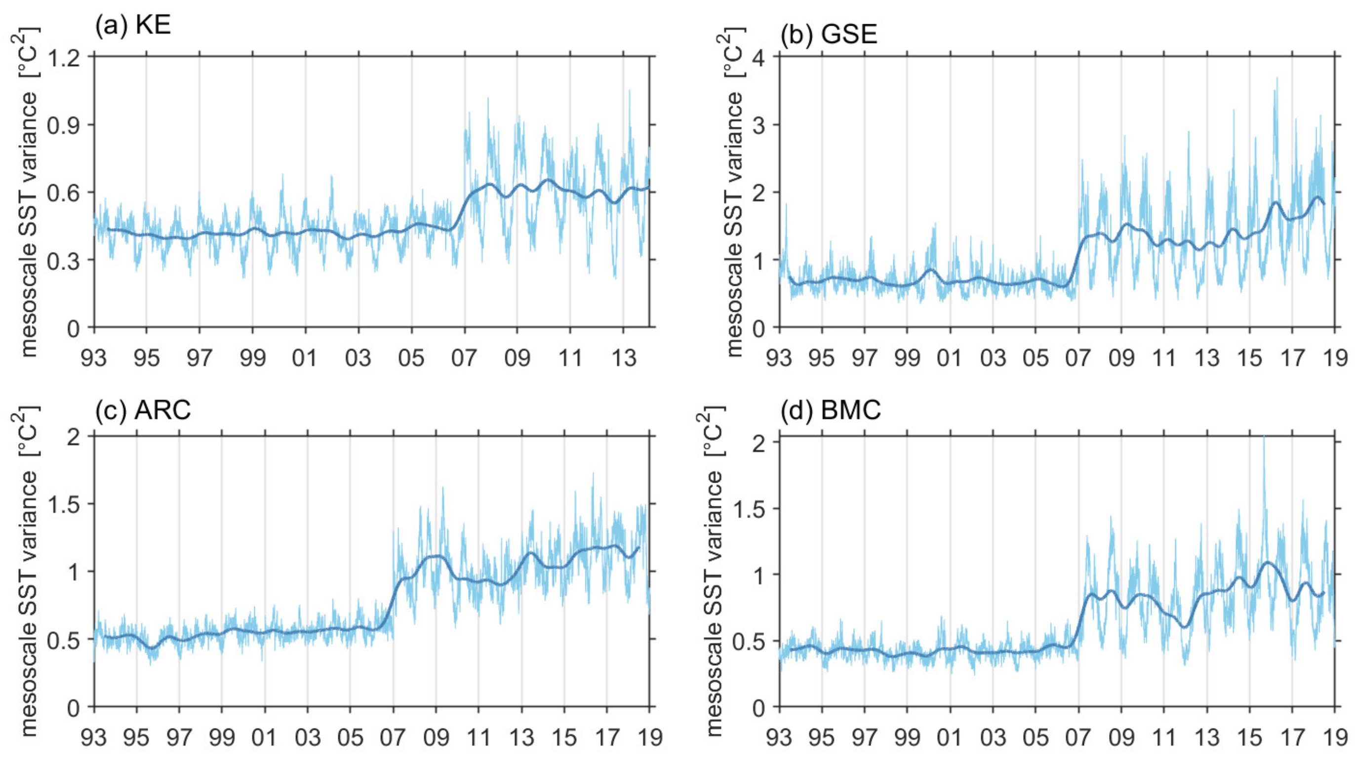
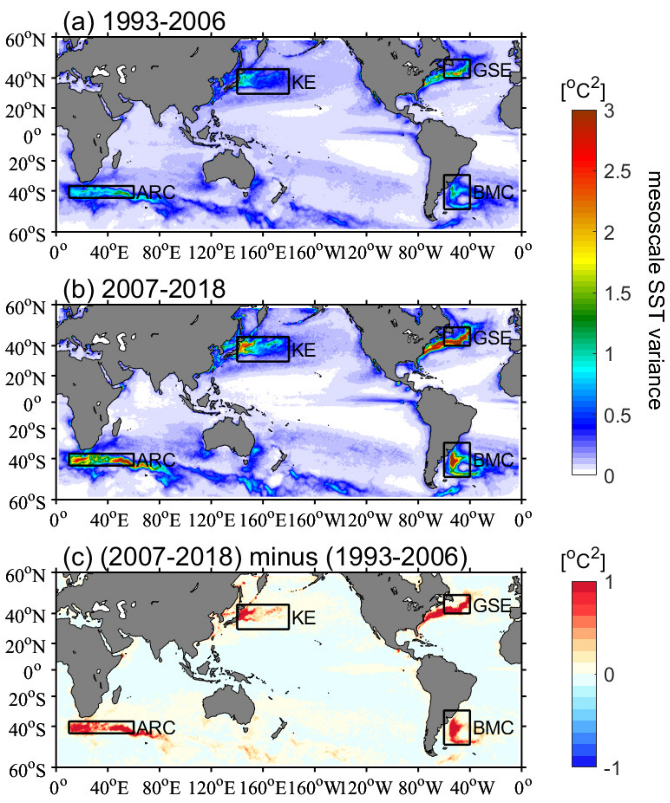
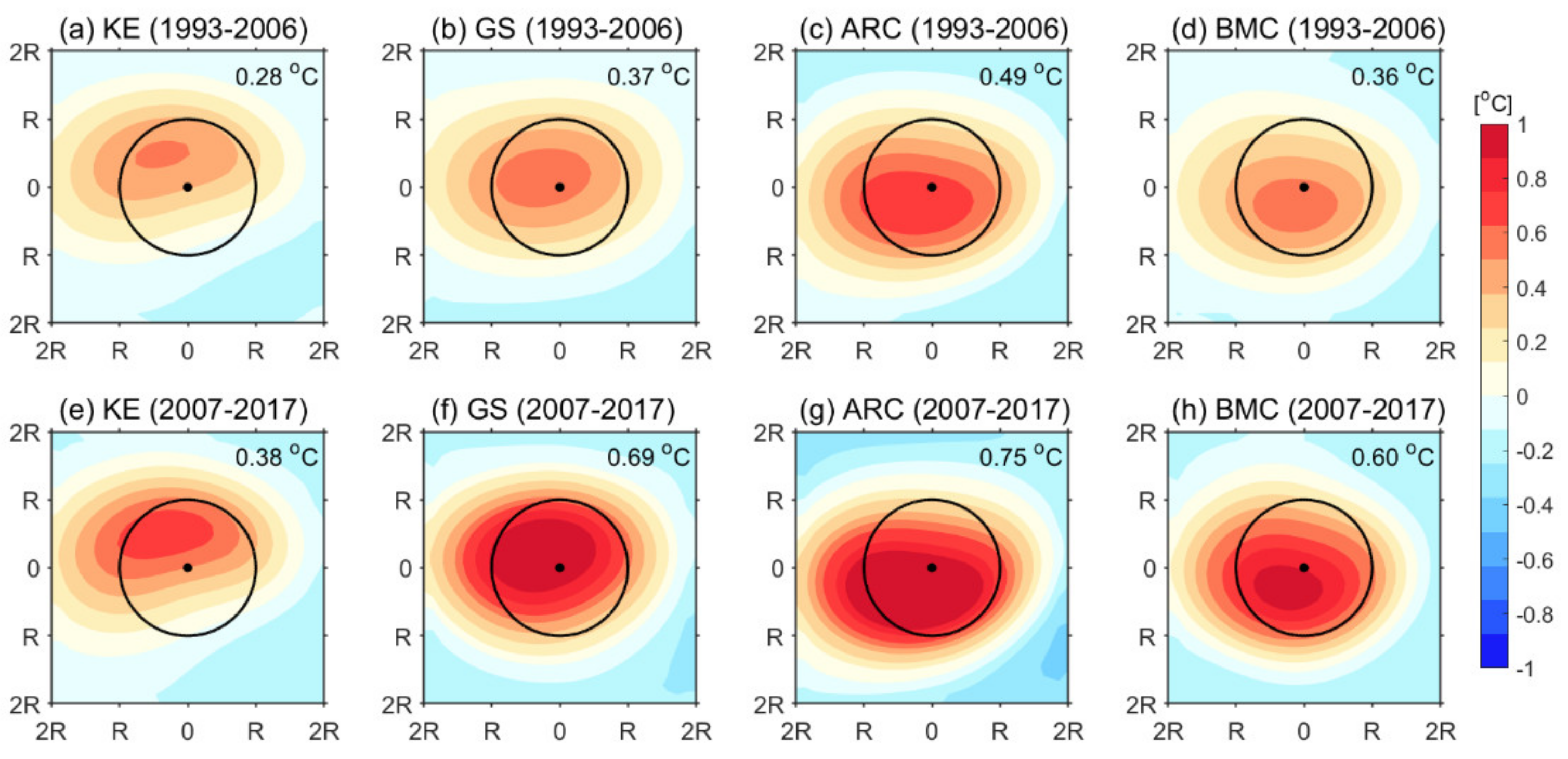
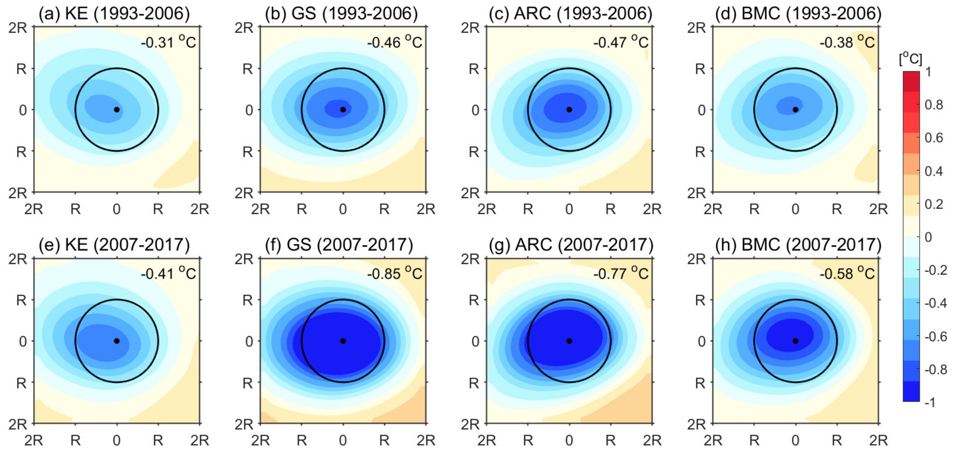
3.1. An Abrupt Increase in Mesoscale SST Variability in 2007

Figure 1 shows the spatial distribution of the mean ${T_{\mathrm{M}}}^{\prime }$ variance derived from the OI.v2-AVHRR-only data during 1993–2018. Notably, the highest levels of mesoscale SST variability are anchored in the subtropical WBCs and their extensions, where are abundant with energetic eddies; this is consistent with previous studies [1,22]. As outlined by the black boxes in Figure 1, the WBCs and their extensions include the Kuroshio Extension (KE; 140°E–180°E, 30°N–45°N), the Gulf Stream Extension (GSE; 40°W–60°W, 40°N–50°N), the Agulhas Return Current (ARC; 10°E–60°E, 37°S–44°S), and the Brazil–Malvinas Confluence (BMC; 40°W–60°W, 30°S–50°S). We refer to “WBCs and their extensions” as “WBC regions” in the following analyses. Among the four WBC regions, the mean ${T_{\mathrm{M}}}^{\prime }$ variance during 1993–2018 in the GSE region is the largest with 1.1 °C² and decreases in the order of the ARC, BMC, and KE regions with values of 0.94 °C², 0.64 °C², and 0.52 °C², respectively. In contrast, ${T_{\mathrm{M}}}^{\prime }$ variance in tropics (20°S–20°N) is typically as small as 0.08 °C². Tropical SST variability is mainly associated with the tropical instability waves (TIWs) with wavelengths of O (1000 km) and large-scale climate models such as the El Niño/Southern Oscillation (ENSO) [71,72]. These signals have been largely attenuated by the 4° × 4° boxcar moving spatial high-pass filter. Therefore, in the following analyses, we will mainly focus on the four WBC regions, where the largest mesoscale air–sea interaction occurred in the global ocean.

To analyze the temporal variability of the intensity of mesoscale SST, the time series of average ${T_{\mathrm{M}}}^{\prime }$ variance in each WBC region derived from the OI.v2-AVHRR-only data are shown in Figure 2. The thin blue lines denote the daily time series, and the thick blue lines denote the 1.5-year low-pass filtered time series. One can see that the ${T_{\mathrm{M}}}^{\prime }$ variance in the four WBC regions exhibits well-defined seasonal variabilities with strong (weak) levels in winter (summer), indicating that the mesoscale air–sea interaction is strongest in winter, which is in agreement with previous studies [13,30,33,37,49]. However, notably, the ${T_{\mathrm{M}}}^{\prime }$ variance in all four WBC regions increased during 1993–2018, and surprisingly, the abrupt increasing points all appeared in 2007. The mean ${T_{\mathrm{M}}}^{\prime }$ variance in the four regions during 2007–2018 is 1.05 °C², which is approximately twofold larger than that during 1993–2006 with 0.54 °C².

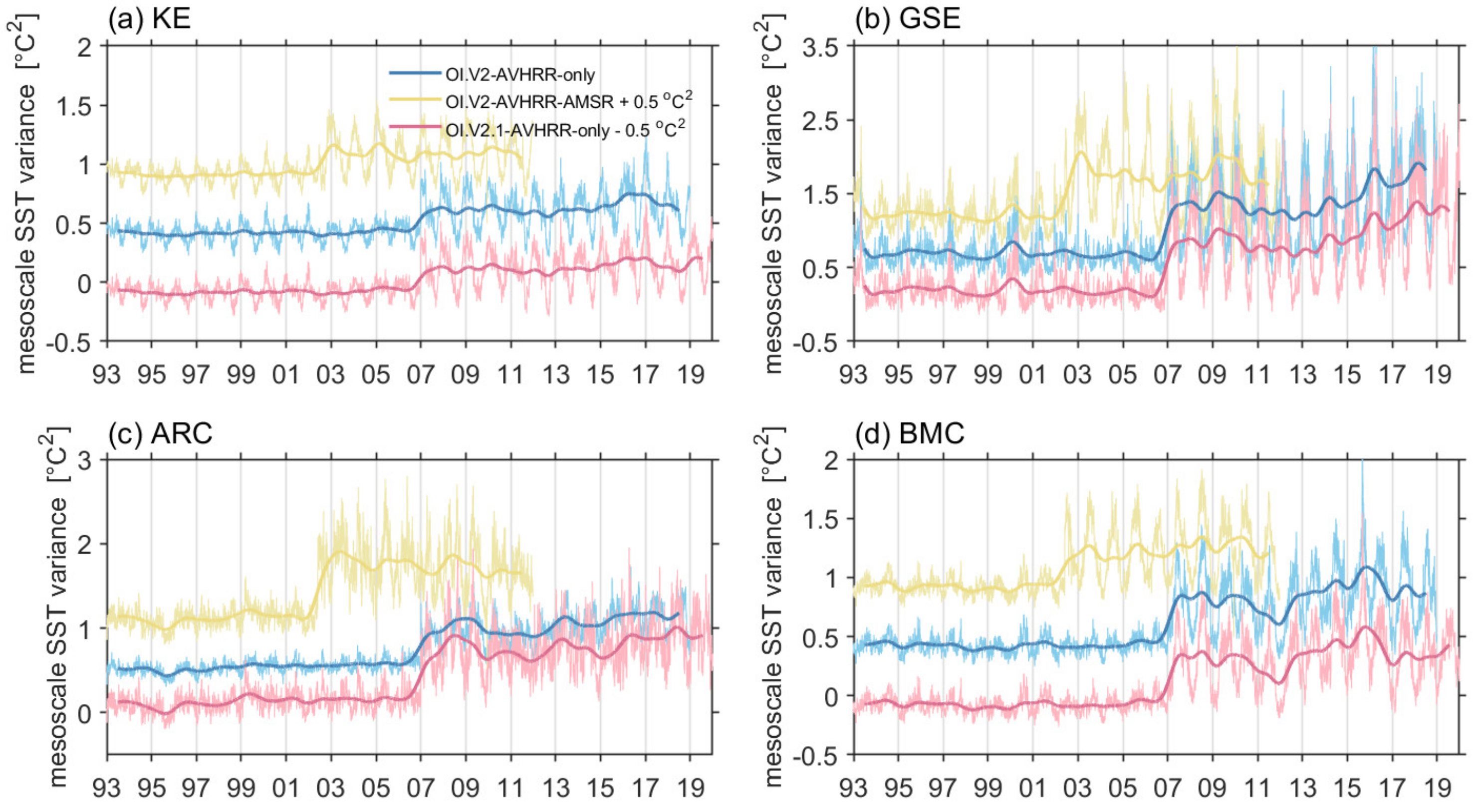
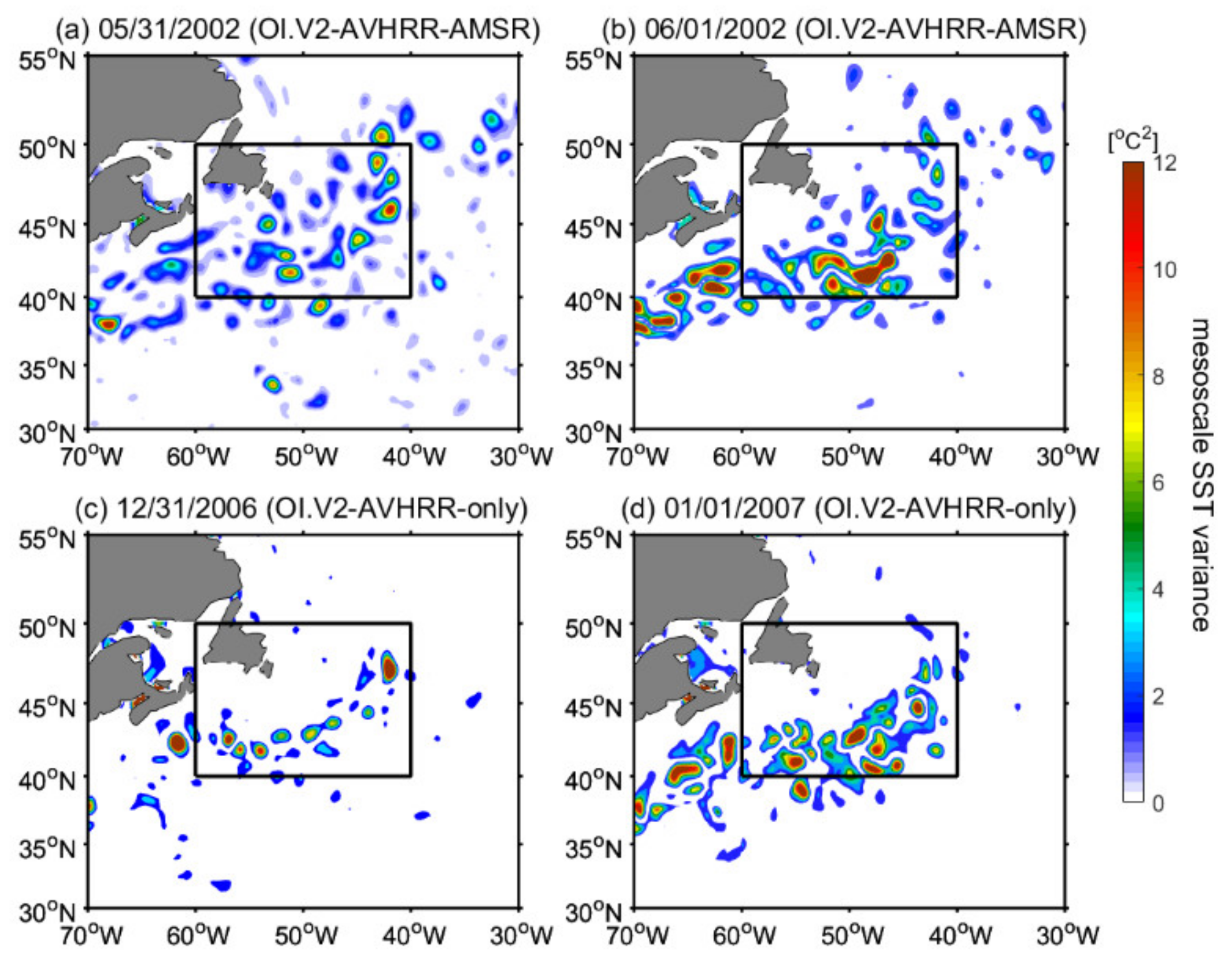
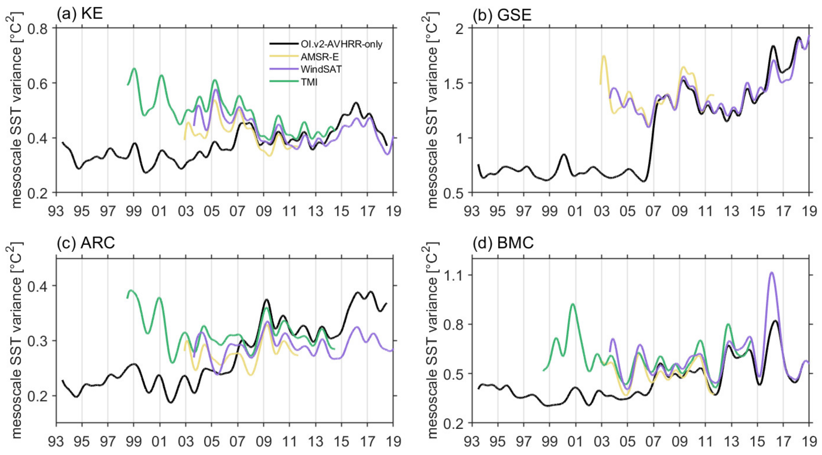
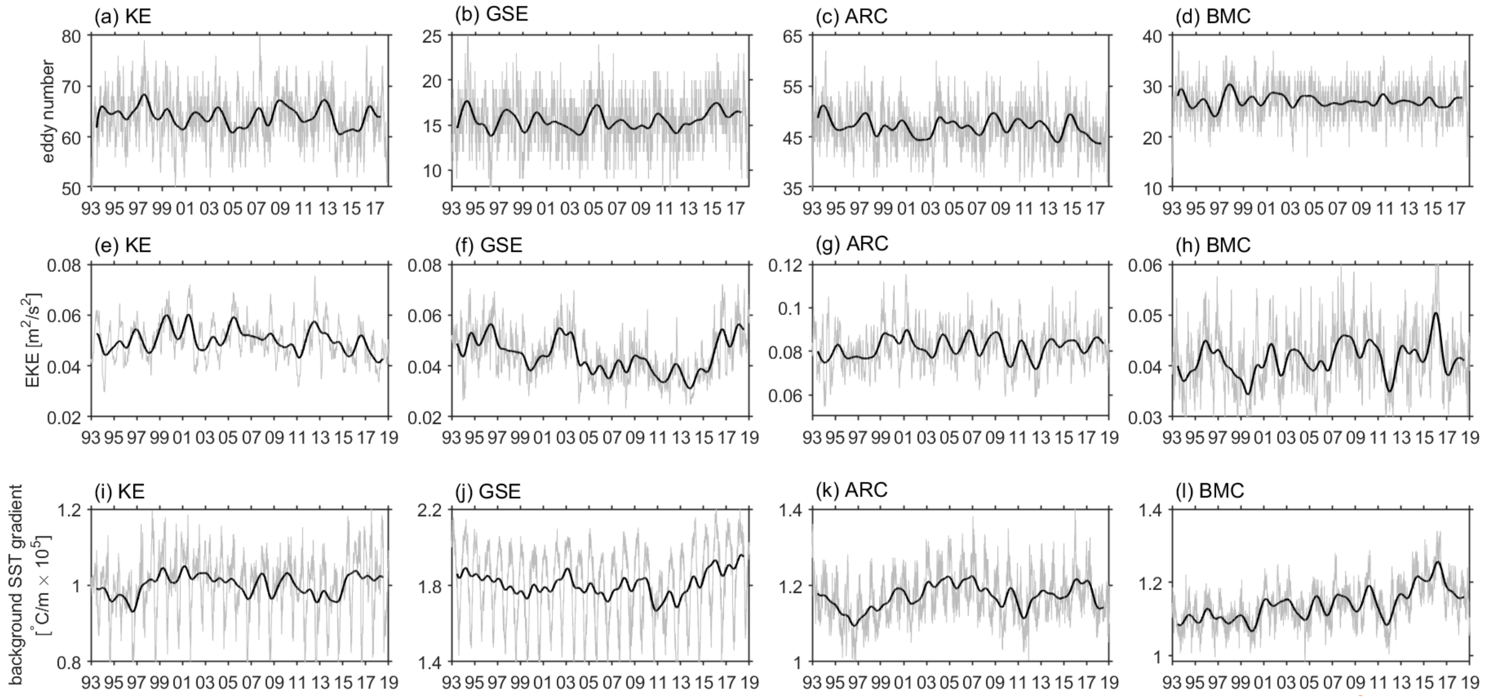
3.2. Causes for the Change

As high-resolution observed SST data, the OI.v2-AVHRR-only data experience widespread use in investigating mesoscale SST signals [40,41,42,43,44,45,46] and are considered as the input of reconstruction of subsurface and deep ocean temperature [55,56,57,58]. Seeking out the reason for the conspicuous abrupt increase in mesoscale SST variability in 2007 is very important to our understanding of the observed mesoscale air–sea interactions. On the one hand, the consistent jump points in 2007 in the four WBC regions may be unveracious due to the different dynamic systems in different regions. On the other hand, if this scenario is reliable, there must be some kind of physical process to regulate it.

We first suspected the validity of the abrupt increase in the ${T_{\mathrm{M}}}^{\prime }$ variance in the four WBC regions in 2007 based on the OI.v2-AVHRR-only data. To examine its credibility, we compared the time series of the $T_{\mathrm{M}}{}^{\prime }$ variance in each region based on the OI.v2-AVHRR-only data with that using the other versions of the OISST data, including OI.v2-AVHRR-AMSR data and OI.v2.1-AVHRR-only data (Figure 3). The thin lines denote the daily time series, and the thick lines denote the 1.5-year low-pass filtered time series. For comparison, the values of $T_{\mathrm{M}}{}^{\prime }$ variance based on OI.v2-AVHRR-AMSR data (yellow lines) and OI.v2.1-AVHRR-only data (red lines) in Figure 3 are the original values plus 0.5 °C² and minus 0.5 °C², respectively. It can be found that the time series of $T_{\mathrm{M}}{}^{\prime }$ variance using OI.v2.1-AVHRR-only data also exhibited enhancement in 2007 in all regions and corresponded well with that using OI.v2-AVHRR-only data (blue lines), which is due to the OI.v2.1-AVHRR-only data before 2016 being the same as OI.v2-AVHRR-only data [62]. However, the most conspicuous discrepancy among these values is that the abrupt increase in the $T_{\mathrm{M}}{}^{\prime }$ variance based on the OI.v2-AVHRR-AMSR data in the four regions all appeared in June 2002, when the AMSR-E instrument was incorporated in the OISST data.

Taking the GSE region as an example, Figure 4a,b show the snapshots of the $T_{\mathrm{M}}{}^{\prime }$ variance on 31 May 2002, and 1 June 2002, respectively, based on OI.v2-AVHRR-AMSR data. The average value of the $T_{\mathrm{M}}{}^{\prime }$ variance in the GSE region (black box in Figure 5a) on 1 June 2002 is 1.52 °C², which is 1.9 times that on 31 May 2002, with 0.79 °C², even on successive days. Similar results are obtained in the OI.v2-AVHRR-only data in 2007. As Figure 4c,d show, based on the OI.v2-AVHRR-only data, the average $T_{\mathrm{M}}{}^{\prime }$ variance in the GSE region on 1 Jan 2007 is 1.47 °C², which is 1.8 times that on 31 Dec 2006, with 0.82 °C², indicating that the abrupt enhancement in 2007 is unveracious due to an artifact in the OI.v2-AVHRR-only data.

To further verify the enhancement of the $T_{\mathrm{M}}{}^{\prime }$ variance in the OI.v2-AVHRR-only data in 2007 is an artifact, we also used other high-resolution satellite SST data including AMSR-E, WindSAT, and TMI data to calculate the $T_{\mathrm{M}}{}^{\prime }$ variance in each WBC region (Figure 5). Compared with the OI.v2-AVHRR-only data, Figure 5 shows the time series of 1.5-year low-pass filtered $T_{\mathrm{M}}{}^{\prime }$ variance based on the different satellite SST data in each region. It is worth noting that as the spatial coverage of the TMI data is confined to 40°S–40°N, the latitudinal bands of KE, ARC, and BMC regions in Figure 5 are defined as 30°N–39°N, 37°S–39°N, and 30°S–39°S, respectively. As the GSE region is outside of 40°S–40°N, Figure 5b lacks the value using TMI data. It can be seen that the $T_{\mathrm{M}}{}^{\prime }$ variance time series exhibit no abrupt enhancement in 2007 using the AMSR-E, WindSAT, and TMI data in all four regions except for that based on the OI.v2-AVHRR-only data, verifying that the jump in the OI.v2-AVHRR-only data is an artifact. Moreover, the values based on the OI.v2-AVHRR-only data are much lower than those using the other satellite SST data before 2007, and all levels of these time series remain roughly consistent in each region after 2007, suggesting that the $T_{\mathrm{M}}{}^{\prime }$ variance based on the OI.v2-AVHRR-only data is underestimated before 2007 and is credible after 2007. Specifically, Figure 6a,b show the mean $T_{\mathrm{M}}{}^{\prime }$ variance during 1993–2006 and 2007–2018, respectively. As shown in the black boxes in Figure 6, in the KE, GSE, ARC, and BMC regions, the mean $T_{\mathrm{M}}{}^{\prime }$ variances during 2007–2018 (1993–2006) are 0.63 (0.42) °C², 1.44 (0.69) °C², 1.29 (0.64) °C², and 0.85 (0.43) °C², respectively. Therefore, the mean $T_{\mathrm{M}}{}^{\prime }$ variance in the KE, GSE, ARC, and BMC regions during 1993–2006 are underestimated by 33%, 52%, 50%, and 49%, respectively. As a result, the mean $T_{\mathrm{M}}{}^{\prime }$ variance in the WBC regions during 1993–2006 is underestimated by 46% compared with that during 2007–2018. Moreover, Figure 6c shows the $T_{\mathrm{M}}{}^{\prime }$ variance anomaly for the periods of 2007–2018 minus 1993-2006. In addition to the four WBC regions with the highest discrepancies, the underestimation before 2007 also exists in the Antarctic Circumpolar Current (ACC), subtropical South Indian Ocean, eastern Australian region, tropical instability wave (TIW) region, and subtropical North Pacific Ocean. In contrast, the $T_{\mathrm{M}}{}^{\prime }$ variance during 1993–2006 is slightly larger than that during 2007–2018 in most tropical regions. Analogously, in the OI.v2-AVHRR-AMSR data, the mean $T_{\mathrm{M}}{}^{\prime }$ variance in the WBC regions before June 2002 is underestimated by 41%, compared with that after June 2002. These results indicate that the OI.v2-AVHRR-only (OI.v2-AVHRR-AMSR) data weakly estimate the strength of the mesoscale SST variation in most subtropical oceans, especially the WBC regions before 2007 (June 2002), due to an artifact in the data.

According to previous studies, we assumed that the jump of mesoscale SST variability in 2007 in the OI.v2-AVHRR-only data is mainly due to the changes in the satellite AVHRR instrument and in situ SST dataset at that time [39,59,60,61]. As

Table 1. Input datasets to the daily OISST data. From [60].

Input Type	Reprocessed or Higher-Quality Data Sets	Operational Data Sets
Satellite (AVHRR SSTs)	Pathfinder 5.0/5.1 (1981–2006)	Navy (2007-present)
In situ SSTs	ICOADS 2.4 (1981–2006)	NCEP (2007-present)
Sea-ice concentrations	GSFC NASA (1981–2004)	NCEP (2005-present)

(from [60]) shows, the AVHRR Pathfinder was used during 1981–2006 and then changed to the operational Navy AVHRR from 2007 to the present. Moreover, the OI.v2-AVHRR-only data were used with the in situ SST data from the International Comprehensive Ocean-Atmosphere Dataset release 2.4 (ICOADS 2.4) during 1981–2006, which changed to the National Centers for Environmental Prediction (NCEP) SST beginning in 2007 and onward. In addition,

Table 2. Platform time spans of AVHRR inputs to the daily OISST data. From [60].

Data Set	Start Date	End Date	Platform	Sensor
Pathfinder	24 August 1981	3 January 1985	NOAA-7	AVHRR/2
	4 January 1985	7 November 1988	NOAA-9	AVHRR/2
	8 November 1988	13 September 1994	NOAA-11	AVHRR/2
	14 September 1994	21 January 1995	NOAA-9	AVHRR/2
	22 January 1995	11 October 2000	NOAA-14	AVHRR/2
	12 October 2000	31 December 2002	NOAA-16	AVHRR/3
	1 January 2003	4 June 2005	NOAA-17	AVHRR/3
	5 Jun 2005	31 December 2006	NOAA-18	AVHRR/3
Navy	1 January 2006	31 December 2008	NOAA-17	AVHRR/3
	1 January 2007	15 August 2011	NOAA-18	AVHRR/3
	1 January 2009	Present	MetOP-A	AVHRR/3
	16 August 2011	Present	NOAA-19	AVHRR/2

(from [60]) shows the platform time spans of AVHRR inputs to the daily OISST data. Only one satellite was available before 2007, and two satellites at a time were used beginning in January 2007, which result in more accuracy of the OI.v2-AVHRR-only data after 2007. Moreover, the observations had sparse spatial coverage before 2007, and most ship observations in the 1985–2006 period were made from insulated buckets, hull contact sensors, and engine condenser intakes at depths of one to several meters [39]. These mentioned reasons may all contribute to the weak estimation of mesoscale SST variability in OI.v2-AVHRR-only data before 2007. Meanwhile, the abrupt enhancement of mesoscale SST variance in June 2002 in the OI.v2-AVHRR-AMSR data is likely due to the incorporation of the AMSR-E product, which is stated in [39] that there existed SST variance jump when the AMSR became available in June 2002. The in situ SST data and observations are the same in the OI.v2-AVHRR-only and OI.v2-AVHRR-AMSR data, suggesting that changes in the satellite AVHRR instrument are the primary factor for the OISST data bias.

We also examined the potential dynamic effects, including the mesoscale eddy number, the EKE, and the background SST gradient (Figure 7). On the one hand, the strength of mesoscale eddies can influence the mesoscale air–sea interaction that stronger eddies correspond to more intense heat transfer between ocean and atmosphere [36]. On the other hand, the mesoscale SST can be generated by the lateral stirring of mesoscale eddies, distorting the background SST, and therefore, the large background SST gradient is favorable for enhanced mesoscale SST [73,74,75]. Figure 7a–d show the eddy numbers in each WBC region based on the mesoscale eddy dataset. The eddy numbers are counted by the daily snapshots of the eddies existing in each region, regardless of whether they are the same eddy on different days. The thin gray lines denote the daily time series, and the thick black lines denote the 1.5-year low-pass filtered time series. It is shown that the eddy numbers remained stable in each region during 1993–2018. In addition, the EKE is calculated by

$$EKE=\frac{g^2}{2f^2}[ {\left(\frac{\partial h^{\prime }}{\partial x}\right)}^2+{\left(\frac{\partial h^{\prime }}{\partial y}\right)}^2]$$

(3)

where $f$ is the Coriolis parameter, g is the gravity constant, and $h^{\prime }$ is the 200-day high-pass filtered SSHA because the oceanic mesoscale eddy signals are associated with temporal scales of 50–200 days [1]. The EKE time series in each WBC region are shown in Figure 7e–h, indicating that the EKE varies with interannual signals except for the abrupt increase in 2007. Notably, changing the high-pass filter to 4° × 4° boxcar moving spatial high-pass filter generates no significant difference in the results. These results rule out that mesoscale eddy variabilities are the reasons for the abrupt increase in mesoscale SST variations in 2007. We further examined the effect of the background SST gradient based on the OI.v2-AVHRR-only data (Figure 7i–l). Similar to calculating EKE, we used the 200-day low-pass filtered SST to represent the background SST, and the background SST gradient can be defined as $\sqrt{{\left(\frac{\partial SST}{\partial x}\right)}^2+{\left(\frac{\partial SST}{\partial y}\right)}^2}$. As shown in Figure 7i–l, in addition to the well-defined seasonal variability, the background SST gradient exhibits interannual variability in each WBC region but without the abrupt increase in 2007, suggesting that the background SST gradient is not responsible for the enhancement of mesoscale SST variability in 2007. The above discussions confirm that the underestimated mesoscale SST variability before 2007 in the OI.v2-AVHRR-only data is an artifact.

3.3. Influence

Considering that the large $T_{\mathrm{M}}{}^{\prime }$ variance corresponds to the intense mesoscale air–sea interaction associated with strong mesoscale eddy-induced SSTA, the underestimated $T_{\mathrm{M}}{}^{\prime }$ variance before 2007 based on the OI.v2-AVHRR-only data is related to the underestimated eddy-induced SSTA. To examine this feature, we matched the mesoscale eddies for each day with the 4° × 4° boxcar moving spatial high-pass filtered SSTA, and Figure 8 shows the composite Anticyclonic Eddy (AE)-induced SSTA in each WBC region during the periods of 1993–2006 and 2007–2017. The composite figures are normalized by the eddy radius, the circles denote the normalized eddy radius and the dots are the eddy centers. It is shown that the composite AE-induced SSTA in the WBC regions exhibits monopole patterns, in agreement with previous studies [21,30,36,37,38]. Moreover, the levels of AE-induced SSTA in all WBC regions during 2007–2017 are overall higher than those during 1993–2006. Similarly, Figure 9 shows the composite Cyclonic Eddy (CE)-induced SSTA in the WBC regions during 1993–2006 and 2007–2017, showing different negative values in these two periods. According to previous studies [11,38], the eddy-induced SSTA can be quantified by the mean SSTA within the eddy radius due to the maximum value that concentrates within the eddy radius. Therefore, the mean AE/CE-induced SSTAs during the two periods in each region can be quantified. The AE (CE)-induced SSTAs in the KE, GS, ARC, and BMC regions during 1993–2006 are 0.28 (−0.31) °C, 0.37 (–0.46) °C, 0.49 (–0.47) °C, and 0.36 (–0.38) °C, respectively, which are underestimated by 26 (24)%, 46 (46)%, 35 (34)%, and 40 (36)%, respectively, compared with those in the corresponding regions during 2007–2017. As a result, the average AE (CE)-induced SSTA in the WBC regions is 0.38 °C (−0.41 °C) during 1993–2006, which is underestimated by 37% (36%), compared with that during 2007–2017, with a value of 0.61 °C (–0.65 °C). Therefore, the underestimated eddy-induced SSTA before 2007 in the WBC regions based on the OI.v2-AVHRR-only data are related to the weak mesoscale air–sea interactions. Similar differences in results are obtained from the OI.v2-AVHRR-AMSR data on the demarcation of June 2002 (figures not shown).

The OISST datasets are appropriate for investigating mesoscale SST, but they are also prevalent in research on large-scale SST variability [20,76,77]. Therefore, it is necessary to examine whether the abrupt enhancement also exists in the large-scale SST variability. Figure 10 shows the area-mean 1.5-year low-pass filtered large-scale SST ($T_{\mathrm{L}}{}^{\prime }$) variance time series in the four WBC regions based on the OI.v2-AVHRR-only data. Noticeably, the $T_{\mathrm{L}}{}^{\prime }$ variance time series demonstrates interannual variability in each WBC region without the abrupt increase in 2007, suggesting that there are no artifacts in the OI.v2-AVHRR-only data when depicting the large-scale SST variability. Similar results are obtained from the OI.v2-AVHRR-AMSR data (figures not shown).

In addition, whether the underestimation of $T_{\mathrm{M}}{}^{\prime }$ variance during 1993–2006 is of importance to the estimation of total (full-scale) SST variance in the WBC regions is not clear. Thus, we could measure the different parts of SST variance in different seasons during 2007–2018 with reference to the value in the period of 1993–2006. We computed the rate of SST variance change in different seasons in each WBC region based on the OI.v2-AVHRR-only data (Figure 11). The seasons of spring (autumn), summer (winter), autumn (spring), and winter (summer) in the Northern (Southern) Hemisphere are defined as March–May, June–August, September–November, and December–February, respectively. Here, as mentioned in the Methods Section, we divided the total SSTA ($T^{\prime }$) into the mesoscale SSTA ($T_{\mathrm{M}}{}^{\prime }$) and large-scale SSTA ($T_{\mathrm{L}}{}^{\prime }$); therefore, we could compute the rate of counterpart SST variance change in each region in different seasons. As Figure 11 shows, the green, red, yellow, and blue bars indicate the different parts of the SST variance change in spring, summer, autumn, and winter, respectively, and the black outlines are the average values of these four seasons. It can be seen that the mean $T_{\mathrm{M}}{}^{\prime }$ variance change in the four seasons (the black outlines in the second column) is overall larger than the mean $T_{\mathrm{L}}{}^{\prime }$ variance change (the black outlines in the third column) in all four WBC regions, indicating that mesoscale SST variability is of great importance to the total SST variability (the black outlines in the first column). Specifically, in the GSE and BMC regions, the mean $T_{\mathrm{M}}{}^{\prime }$ variance during 2007–2018 increased by 35% and 32%, respectively, while the $T_{\mathrm{L}}{}^{\prime }$ variance in the corresponding regions increased by 20% and 15%. However, in the KE and ARC regions, instead of increasing, the $T_{\mathrm{L}}{}^{\prime }$ variance decreased by 7% and 13%, respectively, although the total $T^{\prime }$ variance increased by 4% and 17% (the black outlines in the first column in Figure 11a,c), suggesting that the increase in the total $T^{\prime }$ variance is contributed from the increase in the $T_{\mathrm{M}}{}^{\prime }$ variance due to an artifact in the OI.v2-AVHRR-only data. In addition, the largest underestimation of the $T_{\mathrm{M}}{}^{\prime }$ variance in the WBC regions during 1993–2006 roughly appears in winter (blue bars), except for the GSE region, where the value is slightly larger in spring than in winter. Overall, the mean underestimation of the $T_{\mathrm{M}}{}^{\prime }$ variance during 1993–2006 in the four WBC regions is 36% in winter, which is larger than that in the other seasons and in agreement with previous studies, suggesting that the mesoscale air–sea interaction is stronger in winter [13,30,33,37,49]. Therefore, the above discussions indicate that the underestimation of mesoscale SST variability during 1993–2006 in the WBC regions can influence the estimation of the total SST variability, especially in winter.

The OI.v2-AVHRR-only data and OI.v2-AVHRR-AMSR data play important roles in constructing many other datasets, such as the J-OFURO3 data and CFSR data, that are extensively used in investigating mesoscale eddies [37,78,79]. In the following analysis, we examine whether the $T_{\mathrm{M}}{}^{\prime }$ variance also exhibits an abrupt increase in the WBC regions in the J-OFURO3 data and CFSR data. Figure 12 shows the average $T_{\mathrm{M}}{}^{\prime }$ variance time series in each WBC region during 1993–2013 based on the J-OFURO3 data. Abrupt enhancements can be seen in June 2002 in all regions, which are the same as the results using the OI.v2-AVHRR-AMSR data, as the AMSR data were incorporated in the J-OFURO3 data at that time. The mean $T_{\mathrm{M}}{}^{\prime }$ variance from June 2002 to December 2013 (January 1993 to May 2002) in the KE, GSE, ARC, and BMC regions are 0.43 (0.32) °C², 0.80 (0.45) °C², 0.84 (0.44) °C², and 0.50 (0.31) °C², respectively, indicating that the mean $T_{\mathrm{M}}{}^{\prime }$ variance in the corresponding regions is underestimated by 23%, 44%, 48%, and 38% before June 2002, respectively, based on the J-OFURO3 data. Moreover, these underestimations of the $T_{\mathrm{M}}{}^{\prime }$ variance also exist before June 2002 in the CFSR data (Figure 13). The mean $T_{\mathrm{M}}{}^{\prime }$ variance in the KE, GSE, ARC, and BMC regions from January 1993 to May 2002 is underestimated by 12%, 34%, 37%, and 28%, compared with that from June 2002 to December 2010, respectively. Therefore, the underestimation of mesoscale SST variability also exists in the other SST datasets that are based on the OISST products, which need to be considered when using these data to explore mesoscale SST variability.

4. Conclusions and Discussion

In summary, this study investigated the interannual variability of the intensity of mesoscale SST, which is represented by the mesoscale SST variance in the global ocean, particularly in the four subtropical WBC regions (KE, GSE, ARC, and BMC) for the period of 1993–2018 (Figure 1). The main observed SST data we used were the OISST product, which are widely used to investigate mesoscale SST signals due to their high resolution and long-term temporal coverage. To date, the OISST version 2 (OI.v2) data provide two versions, i.e., OI.v2-AVHRR-only and OI.v2-AVHRR-AMSR. We showed that the time series of the mesoscale SST variance in the four WBC regions all exhibited an abrupt enhancement in 2007 based on the OI.v2-AVHRR-only data (Figure 2), and similar scenarios existed in June 2002 using the OI.v2-AVHRR-AMSR data. By comparing the results based on the OI.v2-AVHRR-only data with those using the other high-resolution satellite SST data, such as the WindSAT, AMSR-E, and TMI data (Figure 5), we showed that there were weak estimations of the mesoscale SST variability in the OI.v2-AVHRR-only data before 2007 in the WBC regions. Specifically, the OI.v2-AVHRR-only data underestimated the mean mesoscale SST variance in the four WBC regions by 46% in the 1993–2006 period, compared with that in the 2007–2018 period (Figure 6). Among the four regions, the largest underestimated mesoscale SST variance during 1993–2006 existed in the GSE region by 52% and decreased in the order of the ARC, BMC, and KE regions by 50%, 49%, and 33%, respectively. Similarly, the mean mesoscale SST variance in the WBC regions based on the OI.v2-AVHRR-AMSR data before June 2002 was underestimated by 41%, compared with that after June 2002. We assumed that these jumps are likely due to an artifact in the OI.v2-AVHRR-only and OI.v2-AVHRR-AMSR data. According to previous studies [39,59,60,61], we assumed that the abrupt enhancement in the mesoscale SST variability in 2007 in the OI.v2-AVHRR-only data is likely mainly due to the change in the satellite AVHRR instrument (Table 1), and the abrupt enhancement of mesoscale SST variability in June 2002 in the OI.v2-AVHRR-AMSR data is likely due to the incorporation of the AMSR-E product. By further examining the potential dynamics underlying this phenomenon, we ruled out the mesoscale eddy number and strength, and therefore, the background SST gradient is responsible for these abrupt enhancements (Figure 7), confirming that the underestimated mesoscale SST variability before 2007 is an artifact of the OI.v2-AVHRR-only data. Notably, the underestimation did not exist in the large-scale SST variance in the WBC regions using OI.v2-AVHRR-only data and OI.v2-AVHRR-AMSR data (Figure 10).

The intensity of mesoscale SST variability was closely associated with the mesoscale eddy-induced SSTA, which triggers the mesoscale air–sea interaction. Thus, the mesoscale eddy-induced SSTA was underestimated based on the OI.v2-AVHRR-only data during 1993–2006 (Figure 8 and Figure 9). Specifically, the average AE (CE)-induced SSTA in the WBC regions was 0.38 (−0.41) °C during 1993–2006, which was underestimated by 37 (36)%, compared with that during 2007–2017, with a value of 0.61 (−0.65) °C. In addition, we also found that the underestimation of mesoscale SST variability can influence the estimation of total SST variability, especially in winter, when the mesoscale air–sea interaction was strongest (Figure 11). As the OI.v2-AVHRR-only and OI.v2-AVHRR-AMSR data are crucial components in the other SST datasets, such as J-OFURO3 data and CFSR data, the underestimated mesoscale SST variability also existed in the J-OFURO3 and CFSR data before June 2002, when the AMSR-E instrument was not incorporated in the OI.v2-AVHRR-AMSR data.

Considering that the OISST products are widely used in exploring the multi-scale SST variability in the global ocean, the weak estimation of mesoscale SST variation before 2007 may influence the evaluation of the observed high-frequency SST signals and extreme climate events. For example, [77] suggests a doubling of the number of marine heatwave days between 1982 and 2016 based on the daily OISST-v.2 dataset. Further analyses are needed to examine marine heatwaves when considering artifacts in the OISST dataset. Moreover, the OISST products, as the high-resolution observed SST datasets, are widely considered the input to reconstruct the oceanic subsurface properties. It is known that the mesoscale signals can penetrate into kilometers in the ocean, especially in the WBC regions [4,7,8,11,49]. The underestimation of mesoscale variability in the OISST products may influence the accuracy of reconstructing three-dimensional oceanic properties. Therefore, it is necessary to take the weak mesoscale SST variability into consideration when using OISST and relevant data products to explore the mesoscale processes.

References

1. Chelton, D.B.; Schlax, M.G.; Samelson, R.M. Global observations of nonlinear mesoscale eddies. Prog. Oceanogr. 2011, 91, 167–216. [Google Scholar] [CrossRef]
2. Von Storch, J.S.; Eden, C.; Fast, I.; Haak, H.; Hernández-Deckers, D.; Maier-Reimer, E.; Stammer, D. An estimate of the Lorenz energy cycle for the world ocean based on the STORM/NCEP simulation. J. Phys. Oceanogr. 2012, 42, 2185–2205. [Google Scholar] [CrossRef]
3. Roemmich, D.; Gilson, J. Eddy transport of heat and thermocline waters in the North Pacific: A key to interannual/decadal climate variability? J. Phys. Oceanogr. 2001, 31, 675–687. [Google Scholar] [CrossRef]
4. Volkov, D.L.; Lee, T.; Fu, L.L. Eddy-induced meridional heat transport in the ocean. Geophys. Res. Lett. 2008, 35, L20601. [Google Scholar] [CrossRef] [Green Version]
5. Wang, X.; Li, W.; Qi, Y.; Han, G. Heat, salt and volume transports by eddies in the vicinity of the Luzon Strait. Deep Sea Res. Part I Oceanogr. Res. Pap. 2012, 61, 21–33. [Google Scholar] [CrossRef]
6. Bishop, S.P.; Watts, D.R.; Donohue, K.A. Divergent eddy heat fluxes in the Kuroshio Extension at 144°–148° E. Part I: Mean structure. J. Phys. Oceanogr. 2013, 43, 1533–1550. [Google Scholar] [CrossRef] [Green Version]
7. Zhang, Z.; Wang, W.; Qiu, B. Oceanic mass transport by mesoscale eddies. Science 2014, 345, 322–324. [Google Scholar] [CrossRef] [PubMed]
8. Dong, C.; McWilliams, J.C.; Liu, Y.; Chen, D. Global heat and salt transports by eddy movement. Nat. Commun. 2014, 5, 3294. [Google Scholar] [CrossRef] [Green Version]
9. Doddridge, E.W.; Marshall, D.P. Implications of eddy cancellation for nutrient distribution within subtropical gyres. J. Geophys. Res. Ocean. 2018, 123, 6720–6735. [Google Scholar] [CrossRef]
10. Huang, J.; Xu, F. Observational Evidence of Subsurface Chlorophyll Response to Mesoscale Eddies in the North Pacific. Res. Lett. Geophys. 2018, 45, 8462–8470. [Google Scholar] [CrossRef] [Green Version]
11. Sun, B.; Liu, C.; Wang, F. Global meridional eddy heat transport inferred from Argo and altimetry observations. Sci. Rep. 2019, 9, 1345. [Google Scholar] [CrossRef] [Green Version]
12. Qiu, B.; Chen, S. Variability of the Kuroshio Extension jet, recirculation gyre, and mesoscale eddies on decadal time scales. J. Phys. Oceanogr. 2005, 35, 2090–2103. [Google Scholar] [CrossRef]
13. O’neill, L.W.; Chelton, D.B.; Esbensen, S.K.; Wentz, F.J. High-resolution satellite measurements of the atmospheric boundary layer response to SST variations along the Agulhas Return Current. J. Clim. 2005, 18, 2706–2723. [Google Scholar] [CrossRef]
14. Kang, D.; Curchitser, E.N. Gulf Stream eddy characteristics in a high-resolution ocean model. J. Geophys. Res. Oceans 2013, 118, 4474–4487. [Google Scholar] [CrossRef]
15. Mason, E.; Pascual, A.; Gaube, P.; Ruiz, S.; Pelegrí, J.L.; Delepoulle, A. Subregional characterization of mesoscale eddies across the Brazil-Malvinas Confluence. J. Geophys. Res. Oceans 2017, 122, 3329–3357. [Google Scholar] [CrossRef] [Green Version]
16. Kelly, K.A.; Small, R.J.; Samelson, R.M.; Qiu, B.; Joyce, T.M.; Kwon, Y.; Cronin, M.F. Western boundary currents and frontal air-sea interaction: Gulf Stream and Kuroshio Extension. J. Clim. 2010, 23, 5644–5667. [Google Scholar] [CrossRef]
17. Talley, L.D.; Pickard, G.L.; Emery, W.J.; Swift, J.H. Descriptive Physical Oceanography: An Introduction, 6th ed.; Elsevier: London, UK, 2011; p. 555. [Google Scholar]
18. Imawaki, S.; Bower, A.S.; Beal, L.; Qiu, B. Western boundary currents. In Ocean Circulation and Climate—A 21st Century Perspective, 2nd ed.; Academic Press: Oxford, UK, 2013; pp. 305–338. [Google Scholar]
19. Small, R.D.; deSzoeke, S.P.; Xie, S.P.; O’neill, L.; Seo, H.; Song, Q.; Cornillon, P.; Minobe, S. Air–sea interaction over ocean fronts and eddies. Dyn. Atmos. Oceans 2008, 45, 274–319. [Google Scholar] [CrossRef]
20. Kwon, Y.O.; Alexander, M.A.; Bond, N.A.; Frankignoul, C.; Nakamura, H.; Qiu, B. Role of the Gulf Stream and Kuroshio-Oyashio systems in large-scale atmosphere-ocean interaction: A review. J. Clim. 2010, 23, 3249–3281. [Google Scholar] [CrossRef]
21. Gaube, P.; Chelton, D.B.; Samelson, R.M.; Schlax, M.G.; O’Neill, L.W. Satellite observations of mesoscale eddy-induced Ekman pumping. J. Phys. Oceanogr. 2015, 45, 104–132. [Google Scholar] [CrossRef]
22. Jing, Z.; Wang, S.; Wu, L.; Chang, P.; Zhang, Q.; Sun, B.; Chen, Z. Maintenance of mid-latitude oceanic fronts by mesoscale eddies. Sci. Adv. 2020, 6, eaba7880. [Google Scholar] [CrossRef]
23. Bishop, S.P.; Small, R.J.; Bryan, F.O.; Tomas, R.A. Scale dependence of midlatitude air–sea interaction. J. Clim. 2017, 30, 8207–8221. [Google Scholar] [CrossRef]
24. Namias, J.; Cayan, D.R. Large-scale air-sea interactions and short-period climatic fluctuatioins. Science 1981, 214, 869–876. [Google Scholar] [CrossRef]
25. Wallace, J.M.; Mitchell, T.P.; Deser, C. The Influence of Sea-Surface Temperature on Surface Wind in the Eastern Equatorial Pacific: Seasonal and Interannual Variability. J. Clim. 1989, 2, 1492–1499. [Google Scholar] [CrossRef]
26. Xie, S.P. Satellite observations of cool ocean atmosphere interaction. Bull. Am. Meteorol. Soc. 2004, 85, 195–208. [Google Scholar] [CrossRef] [Green Version]
27. Okumura, Y.; Xie, S.P. Tropical atlantic air-sea interaction and its influence on the NAO. Geophys. Res. Lett. 2001, 28, 1507–1510. [Google Scholar] [CrossRef] [Green Version]
28. Chelton, D.B.; Schlax, M.G.; Freilich, M.H.; Milliff, R.F. Satellite measurements reveal persistent small-scale features in ocean winds. Science 2004, 303, 978–983. [Google Scholar] [CrossRef] [Green Version]
29. Minobe, S.; Kuwano-Yoshida, A.; Komori, N.; Xie, S.P.; Small, R.J. Influence of the Gulf Stream on the troposphere. Nature 2008, 452, 206–209. [Google Scholar] [CrossRef]
30. Ma, X.; Jing, Z.; Chang, P.; Liu, X.; Montuoro, R.; Small, R.J. Western boundary currents regulated by interaction between ocean eddies and the atmosphere. Nature 2016, 535, 533–537. [Google Scholar] [CrossRef] [PubMed]
31. Shan, X.; Jing, Z.; Gan, B.; Wu, L.; Chang, P.; Ma, X.; Yang, H. Surface heat flux induced by mesoscale eddies cools the Kuroshio-Oyashio Extension region. Geophys. Res. Lett. 2020, 47, e2019GL086050. [Google Scholar] [CrossRef]
32. Shan, X.; Jing, Z.; Sun, B.; Chang, P.; Wu, L.; Ma, X. Influence of the Ocean Mesoscale Eddy–Atmosphere Thermal Feedback on the Upper-Ocean Haline Stratification. J. Phys. Oceanogr. 2020, 50, 2475–2490. [Google Scholar] [CrossRef]
33. Yang, H.; Chang, P.; Qiu, B.; Zhang, Q.; Wu, L.; Chen, Z.; Wang, H. Mesoscale air–sea interaction and its role in eddy energy dissipation in the Kuroshio Extension. J. Clim. 2019, 32, 8659–8676. [Google Scholar] [CrossRef]
34. Yang, H.; Wu, L.; Chang, P.; Qiu, B.; Jing, Z.; Zhang, Q.; Chen, Z. Mesoscale Energy Balance and Air–Sea Interaction in the Kuroshio Extension: Low-Frequency versus High-Frequency Variability. J. Phys. Oceanogr. 2021, 51, 895–910. [Google Scholar] [CrossRef]
35. Pezzi, L.P.; Souza, R.B.; Dourado, M.S. Ocean-atmosphere in situ observations at the Brazil-Malvinas Confluence region. Geophys. Res. Lett. 2005, 32, 312–329. [Google Scholar] [CrossRef] [Green Version]
36. Villas Bôas, A.B.; Sato, O.T.; Chaigneau, A.; Castelão, G.P. The signature of mesoscale eddies on the air-sea turbulent heat fluxes in the south Atlantic ocean. Geophys. Res. Lett. 2015, 42, 1856–1862. [Google Scholar] [CrossRef]
37. Ma, J.; Xu, H.; Dong, C.; Lin, P.; Liu, Y. Atmospheric responses to oceanic eddies in the Kuroshio Extension region. J. Geophys. Res. Atmos. 2015, 120, 6313–6330. [Google Scholar] [CrossRef]
38. Frenger, I.; Gruber, N.; Knutti, R.; Münnich, M. Imprint of Southern Ocean eddies on winds, clouds and rainfall. Nat. Geosci. 2013, 6, 608–612. [Google Scholar] [CrossRef]
39. Reynolds, R.W.; Smith, T.M.; Liu, C.; Chelton, D.B.; Casey, K.S.; Schlax, M.G. Daily high-resolution-blended analyses for sea surface temperature. J. Clim. 2007, 20, 5473–5496. [Google Scholar] [CrossRef]
40. Hausmann, U.; Czaja, A. The observed signature of mesoscale eddies in sea surface temperature and the associated heat transport. Deep Sea Res. Part I Oceanogr. Res. Pap. 2012, 70, 60–72. [Google Scholar] [CrossRef]
41. Frankignoul, C.; Sennechael, N.; Kwon, Y.O.; Alexander, M.A. Influence of the meridional shifts of the kuroshio and the oyashio extensions on the atmospheric circulation. J. Clim. 2011, 24, 762–777. [Google Scholar] [CrossRef]
42. Yuan, Y.; Castelao, R.M. Eddy-induced sea surface temperature gradients in Eastern Boundary Current Systems. J. Geophys. Res. Oceans 2017, 122, 4791–4801. [Google Scholar] [CrossRef]
43. Sun, W.; Dong, C.; Tan, W.; He, Y. Statistical characteristics of cyclonic warm-core eddies and anticyclonic cold-core eddies in the North Pacific based on remote sensing data. Remote Sens. 2019, 11, 208. [Google Scholar] [CrossRef] [Green Version]
44. Liu, Y.; Yu, L.; Chen, G. Characterization of Sea Surface Temperature and Air-Sea Heat Flux Anomalies Associated with Mesoscale Eddies in the South China Sea. J. Geophys. Res. Oceans 2020, 125, e2019JC015470. [Google Scholar] [CrossRef]
45. Martínez-Moreno, J.; Hogg, A.M.; England, M.H.; Constantinou, N.C.; Kiss, A.E.; Morrison, A.K. Global changes in oceanic mesoscale currents over the satellite altimetry record. Nat. Clim. Chang. 2021, 11, 397–403. [Google Scholar] [CrossRef]
46. He, Y.; Feng, M.; Xie, J.; He, Q.; Liu, J.; Xu, J.; Cai, S. Revisit the Vertical Structure of the Eddies and Eddy-Induced Transport in the Leeuwin Current System. J. Geophys. Res. Oceans 2021, 126, e2020JC016556. [Google Scholar] [CrossRef]
47. O’Neill, L.W.; Chelton, D.B.; Esbensen, S.K. Observations of SST-induced perturbations of the wind stress field over the Southern Ocean on seasonal timescales. J. Clim. 2003, 16, 2340–2354. [Google Scholar] [CrossRef] [Green Version]
48. Bryan, F.O.; Tomas, R.; Dennis, J.M.; Chelton, D.B.; Loeb, N.G.; McClean, J.L. Frontal scale air–sea interaction in high-resolution coupled climate models. J. Clim. 2010, 23, 6277–6291. [Google Scholar] [CrossRef]
49. Jing, Z.; Chang, P.; Shan, X.; Wang, S.; Wu, L.; Kurian, J. Mesoscale SST dynamics in the Kuroshio–Oyashio extension region. J. Phys. Oceanogr. 2019, 49, 1339–1352. [Google Scholar] [CrossRef]
50. Yan, X.H.; Okubo, A. Three-dimensional analytical model for the mixed layer depth. J. Geophys. Res. Oceans 1992, 97, 20201–20226. [Google Scholar] [CrossRef]
51. Yan, X.H.; Jo, Y.H.; Liu, W.T.; He, M.X. A new study of the Mediterranean outflow, air–sea interactions, and Meddies using multisensor data. J. Phys. Oceanogr. 2006, 36, 691–710. [Google Scholar] [CrossRef] [Green Version]
52. Wu, X.; Yan, X.H.; Jo, Y.H.; Liu, W.T. Estimation of subsurface temperature anomaly in the North Atlantic using a self-organizing map neural network. J. Atmos. Ocean. Technol. 2012, 29, 1675–1688. [Google Scholar] [CrossRef]
53. Klemas, V.; Yan, X.H. Subsurface and deeper ocean remote sensing from satellites: An overview and new results. Prog. Oceanogr. 2014, 122, 1–9. [Google Scholar] [CrossRef]
54. Qiu, B.; Chen, S.; Klein, P.; Ubelmann, C.; Fu, L.L.; Sasaki, H. Reconstructability of three-dimensional upper-ocean circulation from SWOT sea surface height measurements. J. Phys. Oceanogr. 2016, 46, 947–963. [Google Scholar] [CrossRef]
55. Chapman, C.; Charantonis, A.A. Reconstruction of subsurface velocities from satellite observations using iterative self-organizing maps. IEEE Geosci. Remote Sens. Lett. 2017, 14, 617–620. [Google Scholar] [CrossRef]
56. Su, H.; Li, W.; Yan, X.H. Retrieving temperature anomaly in the global subsurface and deeper ocean from satellite observations. J. Geophys. Res. Oceans 2018, 123, 399–410. [Google Scholar] [CrossRef]
57. Lu, W.; Su, H.; Yang, X.; Yan, X.H. Subsurface temperature estimation from remote sensing data using a clustering-neural network method. Remote Sens. Environ. 2019, 229, 213–222. [Google Scholar] [CrossRef]
58. Meng, L.; Yan, C.; Zhuang, W.; Zhang, W.; Geng, X.; Yan, X.H. Reconstructing High-Resolution Ocean Subsurface and Interior Temperature and Salinity Anomalies from Satellite Observations. IEEE Trans. Geosci. Remote Sens. 2021, 99, 1–14. [Google Scholar] [CrossRef]
59. Woodruff, S.D.; Worley, S.J.; Lubker, S.J.; Ji, Z.; Eric Freeman, J.; Berry, D.I.; Wilkinson, C. ICOADS Release 2.5: Extensions and enhancements to the surface marine meteorological archive. Int. J. Climatol. 2011, 31, 951–967. [Google Scholar] [CrossRef] [Green Version]
60. Banzon, V.; Smith, T.M.; Chin, T.M.; Liu, C.; Hankins, W. A long-term record of blended satellite and in situ sea-surface temperature for climate monitoring, modeling and environmental studies. Earth Syst. Sci. Data 2016, 8, 165–176. [Google Scholar] [CrossRef] [Green Version]
61. Huang, B.; Liu, C.; Banzon, V.F.; Zhang, H.M.; Karl, T.R.; Lawrimore, J.H.; Vose, R.S. Assessing the impact of satellite-based observations in sea surface temperature trends. Geophys. Res. Lett. 2016, 43, 3431–3437. [Google Scholar] [CrossRef] [Green Version]
62. Huang, B.; Liu, C.; Banzon, V.; Freeman, E.; Graham, G.; Hankins, B.; Zhang, H.M. Improvements of the daily optimum interpolation sea surface temperature (DOISST) version 2.1. J. Clim. 2021, 34, 2923–2939. [Google Scholar] [CrossRef]
63. Kummerow, C.; Barnes, W.; Kozu, T.; Shiue, J.; Simpson, J. The tropical rainfall measuring mission (TRMM) sensor package. J. Atmos. Ocean. Technol. 1998, 15, 809–817. [Google Scholar] [CrossRef]
64. Wentz, F.J.; Ricciardulli, L.; Gentemann, C.; Meissner, T.; Hilburn, K.A.; Scott, J. Remote Sensing Systems Coriolis WindSat Daily Environmental Suite on 0.25 deg Grid, Version 7.0.1. 2013. Available online: www.remss.com/missions/windsat (accessed on 12 January 2022).
65. Dong, S.; Gille, S.T.; Sprintall, J.; Gentemann, C. Validation of the Advanced Microwave Scanning Radiometer for the Earth Observing System (AMSR-E) sea surface temperature in the Southern Ocean. J. Geophys. Res. Oceans 2006, 111, 1–16. [Google Scholar] [CrossRef]
66. Tomita, H.; Hihara, T.; Kako, S.I.; Kubota, M.; Kutsuwada, K. An introduction to J-OFURO3, a third-generation Japanese ocean flux data set using remote-sensing observations. J. Oceanogr. 2019, 75, 171–194. [Google Scholar] [CrossRef] [Green Version]
67. Saha, S.; Moorthi, S.; Pan, H.L.; Wu, X.; Wang, J.; Nadiga, S.; Goldberg, M. The NCEP climate forecast system reanalysis. Bull. Am. Meteorol. Soc. 2010, 91, 1015–1058. [Google Scholar] [CrossRef]
68. Taburet, G.; Sanchez-Roman, A.; Ballarotta, M.; Pujol, M.I.; Legeais, J.F.; Fournier, F.; Dibarboure, G. DUACS DT2018: 25 years of reprocessed sea level altimetry products. Ocean Sci. 2019, 15, 1207–1224. [Google Scholar] [CrossRef] [Green Version]
69. Schlax, M.G.; Chelton, D.B. The “growing method” of eddy identification and tracking in two and three dimensions. College of Earth, Oregon State University, Corvallis, Oregon, 8. Ocean Atmos. Sci. 2016. Available online: https://www.aviso.altimetry.fr/fileadmin/documents/data/products/value-added/Schlax_Chelton_2016.pdf (accessed on 12 January 2022).
70. Schlax, M.G.; Chelton, D.B. Frequency domain diagnostics for linear smoothers. J. Am. Stat. Assoc. 1992, 87, 1070–1081. [Google Scholar] [CrossRef]
71. Neelin, J.D.; Battisti, D.S.; Hirst, A.C.; Jin, F.F.; Wakata, Y.; Yamagata, T.; Zebiak, S.E. ENSO theory. J. Geophys. Res. Oceans 1998, 103, 14261–14290. [Google Scholar] [CrossRef]
72. Jansen, M.F.; Dommenget, D.; Keenlyside, N. Tropical atmosphere–ocean interactions in a conceptual framework. J. Clim. 2009, 22, 550–567. [Google Scholar] [CrossRef]
73. Gaube, P.; McGillicuddy, D.J., Jr.; Chelton, D.B.; Behrenfeld, M.J.; Strutton, P.G. Regional variations in the influence of mesoscale eddies on near-surface chlorophyll. J. Geophys. Res. Oceans 2014, 119, 8195–8220. [Google Scholar] [CrossRef] [Green Version]
74. Frenger, I.; Münnich, M.; Gruber, N.; Knutti, R. Southern Ocean eddy phenomenology. J. Geophys. Res. Oceans 2015, 120, 7413–7449. [Google Scholar] [CrossRef] [Green Version]
75. Amores, A.; Melnichenko, O.; Maximenko, N. Coherent mesoscale eddies in the North Atlantic subtropical gyre: 3-D structure and transport with application to the salinity maximum. J. Geophys. Res. Oceans 2017, 122, 23–41. [Google Scholar] [CrossRef]
76. Lima, F.P.; Wethey, D.S. Three decades of high-resolution coastal sea surface temperatures reveal more than warming. Nat. Commun. 2012, 3, 704. [Google Scholar] [CrossRef] [PubMed] [Green Version]
77. Frölicher, T.L.; Fischer, E.M.; Gruber, N. Marine heatwaves under global warming. Nature 2018, 560, 360–364. [Google Scholar] [CrossRef] [PubMed]
78. Yang, P.; Jing, Z.; Wu, L. An assessment of representation of oceanic mesoscale eddy-atmosphere interaction in the current generation of general circulation models and reanalyses. Geophys. Res. Lett. 2018, 45, 11856–11865. [Google Scholar] [CrossRef]
79. Ji, J.; Ma, J.; Dong, C.; Chiang, J.C.; Chen, D. Regional dependence of atmospheric responses to oceanic eddies in the North Pacific Ocean. Remote Sens. 2020, 12, 1161. [Google Scholar] [CrossRef] [Green Version]
Figure 1. Mean mesoscale SST variance distribution derived from OI.v2-AVHRR-only data during 1993–2018. The black boxes denote the Kuroshio Extension (KE, 140°E–180°E, 30°N–45°N), the Gulf Stream Extension (GSE, 40°W–60°W, 40°N–50°N), the Agulhas Return Current (ARC, 10°E–60°E, 37°S–44°S), and the Brazil–Malvinas Confluence (BMC, 40°W–60°W, 30°S–50°S), respectively.
Remotesensing 14 00409 g001
Figure 2. Time series of the mesoscale SST variance based on the OI.v2-AVHRR-only data in the regions of (a) KE, (b) GSE, (c) ARC, and (d) BMC. The thin and thick lines denote the daily and 1.5-year low-pass filtered time series, respectively.
Remotesensing 14 00409 g002
Figure 3. Time series of the mesoscale SST variance in the (a) KE, (b) GSE, (c) ARC, and (d) BMC regions. The blue, yellow, and red lines denote the values based on the OI.V2-AVHRR-only data, OI.v2-AVHRR-AMSR data, and OI.v2.1-AVHRR-only data, respectively. For comparison, the yellow (red) line is the original value plus (minus) 0.5 °C2. The thin and thick lines denote the daily and 1.5-year low-pass filtered time series, respectively.
Remotesensing 14 00409 g003
Figure 4. The snapshots of mesoscale SST variance in the GSE region based on the (a,b) OI.V2-AVHRR-AMSR data on (a) 31 May 2002 and (b) 1 June 2002; (c,d) OI.v2-AVHRR-only data on (c) 31 December 2006 and (d) 1 January 2007.
Remotesensing 14 00409 g004
Figure 5. Time series of the 1.5-year low-pass filtered mesoscale SST variance in the (a) KE, (b) GSE, (c) ARC, and (d) BMC regions. The black, yellow, purple, and green lines denote the value based on the OI.v2-AVHRR-only data, AMSR-E data, WindSAT data, and TMI data, respectively.
Remotesensing 14 00409 g005
Figure 6. Mean mesoscale SST variance distribution derived from OI.v2-AVHRR-only data during the periods of (a) 1993–2016, (b) 2007–2018, and (c) 2007–2018 minus 1993–2016.
Remotesensing 14 00409 g006
Figure 7. Time series of (ad) eddy numbers, (e,f) eddy kinetic energy (EKE), and (il) background SST gradient in the (a,e,i) KE, (b,f,j) GSE, (c,g,k) ARC, and (d,h,l) BMC regions. The thin and thick lines denote the daily and 1.5-year low-pass filtered time series, respectively.
Remotesensing 14 00409 g007
Figure 8. The composite Anticyclonic Eddy (AE)-induced SSTA in the (a,e) KE, (b,f) GSE, (c,g) ARC, and (d,h) BMC regions during the periods of (ad) 1993–2006, and (eh) 2007–2017 based on the OI.v2-AVHRR-only data. The circles denote the normalized eddy radius, and the dots are the eddy centers.
Remotesensing 14 00409 g008
Figure 9. The same as Figure 8, except for the Cyclonic Eddy (CE)-induced SSTA.
Remotesensing 14 00409 g009
Figure 10. Time series of the 1.5-year low-pass filtered large-scale SST variance in the (a) KE, (b) GSE, (c) ARC, and (d) BMC regions based on the OI.v2-AVHRR-only data.
Remotesensing 14 00409 g010
Figure 11. The rate of total, mesoscale, and large-scale SST variance change during 2007–2018, compared with the period of 1993–2006 in different seasons in the (a) KE, (b) GSE, (c) ARC, and (d) BMC regions based on the OI.v2-AVHRR-only data. The green, red, yellow, and blue bars denote the seasons of spring, summer, autumn, and winter, respectively. The black outlines are the average values of the four seasons.
Remotesensing 14 00409 g011
Figure 12. Time series of the mesoscale SST variance based on the J-OFURO3 data in the regions of (a) KE, (b) GSE, (c) ARC, and (d) BMC. The thin and thick lines denote the daily and 1.5-year low-pass filtered time series, respectively.
Remotesensing 14 00409 g012
Figure 13. Time series of the mesoscale SST variance based on the CFSR data in the regions of (a) KE, (b) GSE, (c) ARC, and (d) BMC. The thin and thick lines denote the daily and 1.5-year low-pass filtered time series, respectively.
Remotesensing 14 00409 g013