Consistency Analysis of the GNSS Antenna Phase Center Correction Models

Abstract

For the same antenna type, numerical differences among the phase center correction (PCC) models released by different institutes can reach several millimeters, which is far beyond the nominal calibration accuracy. This contribution introduces a new method to evaluate the consistency of these PCC models. We first investigated the coupling of phase center offset (PCO) and phase center variation (PCV) through simulation experiments, and the results show that the calibrated PCO values under different strategies may result in large differences, and so do PCV values due to strong coupling with PCO. This is further confirmed by field calibration experiments. Moreover, a new datum parameter is introduced to equivalently transform the PCC models to assess the consistency of PCC models of the same antenna type calibrated under different strategies or by different facilities. It is also essential to perform consistency analysis of PCC models in the coordinate domain. We further investigated these PCC models through a simulated positioning experiment. The results show that millimeter-level consistency of PCC models will lead to the same level of positioning precision in the coordinate domain. Moreover, as a comparison, both baseline positioning and PPP were performed with an antenna-type JAV_RINGANT_G3T NONE based on real observations. Multiday results showed that the average RMS of the positioning differences between PCC models from robot and anechoic chamber calibration is less than 1 mm for the baseline solution and 4 mm for the PPP solution, although the PCC model differences can reach 6 mm in L1 and 4 mm in L2, respectively. Finally, we also investigated the distribution of position biases without PCC or with inaccurate PCC. Considering the actual GPS constellation, we found that position biases have a strong correlation with latitude, if PCV values fluctuate greatly with the users’ elevation angle.

1. Introduction

With the development of the Global Navigation Satellite System (GNSS) and the emergence of more high-precision applications, more sophisticated models are required to address various errors, and the antenna phase center correction model is one of these vital models.

Phase center correction (PCC) aims to address the range error caused by the antenna phase center variation when transmitting and receiving GNSS signals. In the signal processing of an antenna, the real reception points of signals from different directions do not form an ideal hemisphere, which will cause delays or advances in phase observation. The PCC magnitude can reach the decimeter level according to the antenna structure. Therefore, the PCC model must be carefully handled in applications where phase observations are involved.

In recent decades, various efforts have been devoted to calibrating PCC models. The initial antenna calibration is performed in an anechoic chamber [1,2,3] using simulated signals. Anechoic chamber calibration is viewed as a high-precision method. In the late 1990s, Mader [4] proposed a new kind of calibration method at the National Geodetic Survey (NGS) using a short baseline in the field. In this calibration, a specified Dorne Margolin choke ring antenna (AOAD/M_T) was assumed as the reference, and the PCC models to be estimated were all relative to this reference antenna. In addition, due to the static antenna and a similar satellite trajectory, this relative calibration cannot provide a full antenna phase center pattern with respect to both the elevation and azimuth angle. Wübbena et al. [5] and Menge et al. [6] proposed an absolute antenna calibration using an industrial robot. Benefiting from the swift motion of the robot, an absolute model is available and is free from the reference antenna.The absolute calibration model has been adopted by the International GNSS Service (IGS), and several institutions have provided absolute antenna calibration services.

In recent years, studies on the influences of the PCC model have drawn much attention. Bergstrand et al. [7] proposed a new method to evaluate the impact of the PCC model on the positioning. Krzan et al. [8] compared the differences between PCC models from field and chamber calibration for the same antenna. Darugna et al. [9] assessed the impact of absolute smartphone antenna calibration on high-precision positioning. Villiger et al. [10] studied GNSS scale determination with antenna patterns for the Galileo system.

2. Phase Center Correction Model

2.1. Phase Center Model

The PCC model [11] widely adopted by the GNSS community is shown in Figure 1. In the spatial hemisphere above the antenna, an accessible point is defined as the antenna reference point (ARP), and a three-dimensional vector from the ARP to the average phase receiving center is defined as the phase center offset (PCO), and the range variation in the phase observation in different directions based on PCO is defined as the phase center variation (PCV). PCC is described in the antenna body system. The x-axis of the frame points from ARP to the north reference marker (NRP) of the antenna while the z-axis points from ARP to the boresight of the antenna. The y-axis together with the x-axis and z-axis form a left-hand coordinate system. If the antenna is placed at a station and oriented correctly, the antenna system is aligned to the local north-east-up system of the station. According to this PCC model, users can correct the phase observation while considering the relative attitude between the satellite and ground antenna. With the help of PCC models, GNSS-based applications with different antennas can reach a clear and consistent solution, which can reduce systematic bias and improve the positioning accuracy.

Considering that the wavefront of all signals can form a series of concentric circles, range deviations from two arbitrary wavefronts with certain distances are equivalent in any direction. It is necessary to consider this kind of constant range bias to construct a comprehensive understanding of the PCC model. Therefore, in addition to the traditional PCO/PCV sets, another datum parameter, denoted as B, is introduced in this contribution to help the analysis and evaluation of the PCC model. It should be emphasized that this datum B in the PCC model will not affect the position estimates. In single point positioning, B will be perfectly absorbed into the receiver clock or ambiguity while in relative positioning, B will be eliminated if differencing between satellites is performed. In this contribution, B is used as a tool to aid in evaluating and analyzing the PCC model.

The computation of PCC can be expressed as:

$$PCC\left(\alpha ,z\right)=-PCO\cdot e+PCV\left(\alpha ,z\right)+B$$

(1)

where PCO is a three-dimensional vector in local north-east-up coordinates, and PCV is a range correction, usually in a tabular format. Thus, PCV needs to be interpolated through values at surrounding grid points; B is the unknown datum constant; e denotes the directional vector from the ground antenna to the satellite. α and z denote the azimuth and zenith angles, respectively, and e can be expressed by α and z as:

$$e=\left\{\sin \left(z\right)·\cos \left(\alpha \right),\sin \left(z\right)·\sin \left(\alpha \right),\cos \left(z\right)\right\}$$

(2)

In the typical PCC model concept, it is assumed that no deviation exists in the zenith direction, which means that B is zero. When using the PCC model, this practice will not affect the position estimates while in antenna calibration, a zero PCV constraint in the zenith direction is one of the necessary demands for the PCV estimation to set a PCV datum and avoid rank defects of the normal equation. In other words, a constraint of B as 0 in the zenith direction is reasonable and feasible in practice, although B might not be zero. It will make sense when transforming the PCC model from a set of PCO/PCV to another set while keeping the consistency between them, and their coupling features will be investigated in the following sections.

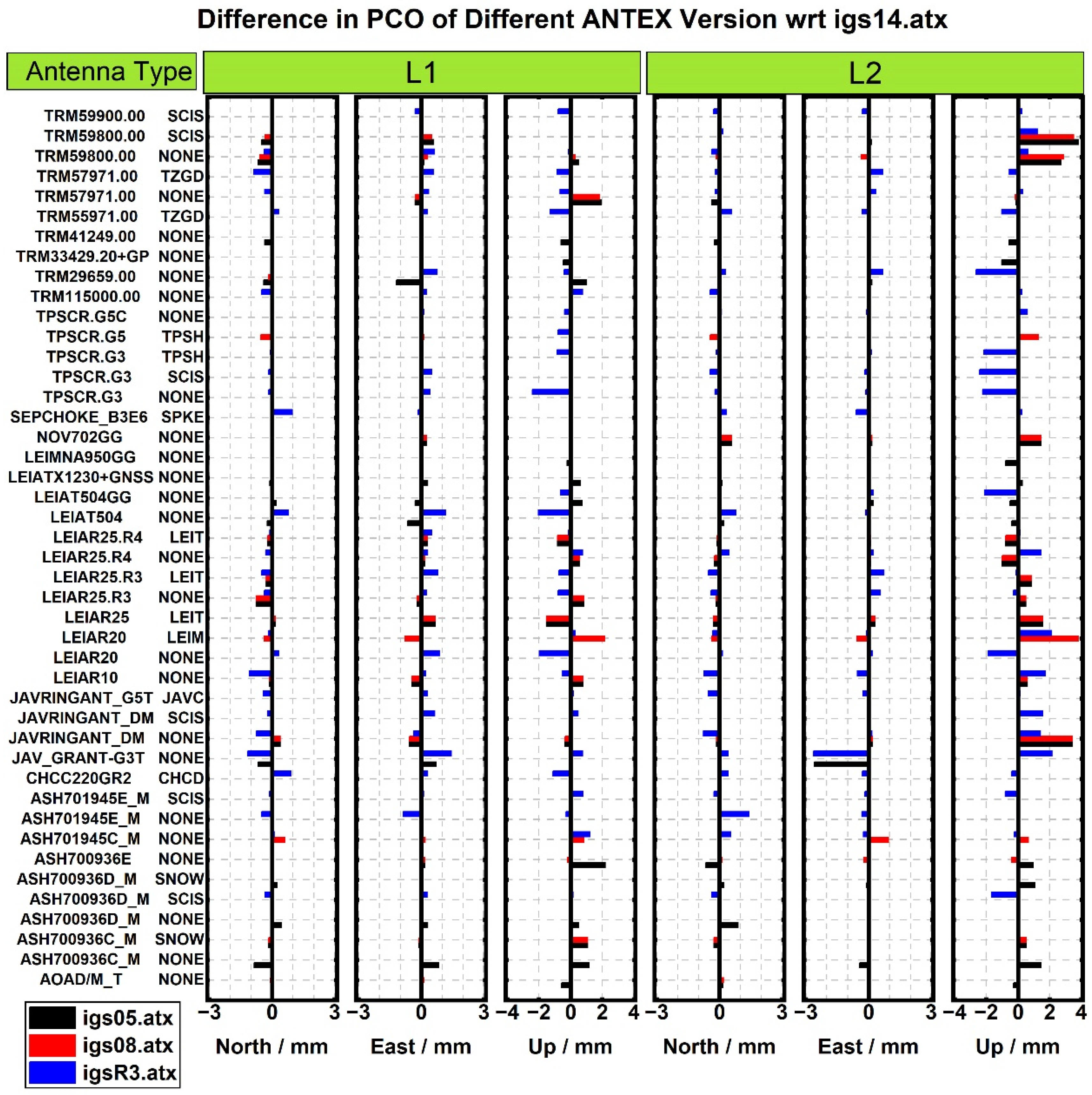
2.2. Differences in Different IGS ANTEX Versions

At present, several institutions have accomplished antenna field calibration and released PCC models in research or commercial methods, including Geo++ [12], NGS [13], Institut für Erdmessung, Leibniz University Hannover (IfE) [14], Geoscience Australia [15], and Senatsverwaltung für Stadtentwicklung und Wohnen (SenStadt), Berlin. However, differences do exist between PCC models from different institutions and calibration methods [7]. As the largest GNSS research community, the IGS also adopts more than 300 PCC models from those institutions and releases them to promote GNSS research. Since 2005, igs05.atx, igs08.atx, and igs14.atx have been successively released by the IGS, which are in accordance with the corresponding International Terrestrial Reference Frame (ITRF). In 2019, IGS released igsR3.atx as a part of the ReProcess3 Campaign that comprises the newest PCC models of multi-GNSS and multifrequency [10]

Investigating the PCC models released by IGS, differences in PCOs with a magnitude exceeding 1 mm can be found for some receiver antennas between different versions of the antenna file in the antenna exchange format (ANTEX) [16]. Taking igs14.atx as a reference, PCO differences in the robot calibration models from igs05.atx, igs08.atx, and igsR3.atx have been calculated and are shown in Figure 2. For more than 40 PCC models, the magnitudes of the PCO shifts among different versions exceeds 1 mm. In general, the shifts in the north and east components are less than or approximately 1 mm except for antenna JAV_GRANT-G3T NONE. The PCO shifts in the up component can reach 4 mm, which are comparably larger. In addition, it can be seen in Figure 2 that the magnitude of the PCO shift with an L2 frequency is larger than that with L1, which may imply that a higher precision and stability of the PCC model in L1 can be expected compared with L2. The PCO estimates are quite stable, and the repeatability of calibration is better than 1 mm or even 0.5 mm. This contradiction may cause some confusion and undermine the user’s confidence in the consistency of PCC models.

In the comparison, an extreme example of a PCC model for the antenna type JAV_RINGANT_G3T NONE is found between robot calibration from igs14.atx and anechoic chamber calibration from igsR3.atx. As listed in

Table 1. Differences between igs14.atx and igsR3.atx of PCO and datum B for Antenna JAV_RINGANT_G3T NONE (unit:mm).

PCC	L1				L2
	N	E	U	B (PCVz = 0)	N	E	U	B (PCVz = 0)
igs14.atx	0.25	2.24	49.04	0	6.80	−3.16	54.72	0
igsR3.atx	0.46	2.19	55.06	3	6.25	−2.97	58.58	2.46
Difference	−0.21	0.05	−6.02	−3	0.55	−0.19	−3.86	−2.46

, the numerical differences in PCO in L1 and L2 apparently exceed 1 mm. Taking the differences in L1 as an example, differences in the north, east, and up components reach (−0.21, 0.05, −6.02) mm, respectively. The convention of $PCV\left(\alpha ,z\right){|}_{z=0}=0$ is not followed by the anechoic chamber calibration, and datum of 3 mm can be found. Therefore, these two models are quite different and a low consistency between them is seen in the elevation-dependent PCV shown in Figure 3. We will investigate the consistency of this example in detail in the following section.

Considering the variations and discrepancies shown in the previous context, it may cause problems for users when choosing an appropriate PCC model. This contribution focuses on the analysis and investigation of the correlation of PCO/PCV sets and aims to find a proper method to evaluate PCC models, including the consistency and impact on positioning.

3. Methodologies and Experiment Design

Motivated by the relatively large difference between different PCC models for the same antenna, we designed the simulation experiment described in the following subsection to investigate the possible reason for this difference and how to evaluate the consistency between these models.

The analysis and evaluation of the PCC model are mainly based on two simulation experiments of PCC estimation and point positioning. In the simulation of PCC estimation, virtual dPCC observations are constructed from the original PCC model released by IGS, and then new PCC models are estimated with different strategies. In the simulated positioning experiment, virtual ranging observations are constructed from two PCC models, and point positioning is performed to evaluate the differences in the two PCC models in the coordinate domain. In this section, we mainly introduce our methodologies and the design of the simulation experiment for PCC estimation and positioning as shown in Figure 4, and the details will be described in the following sections.

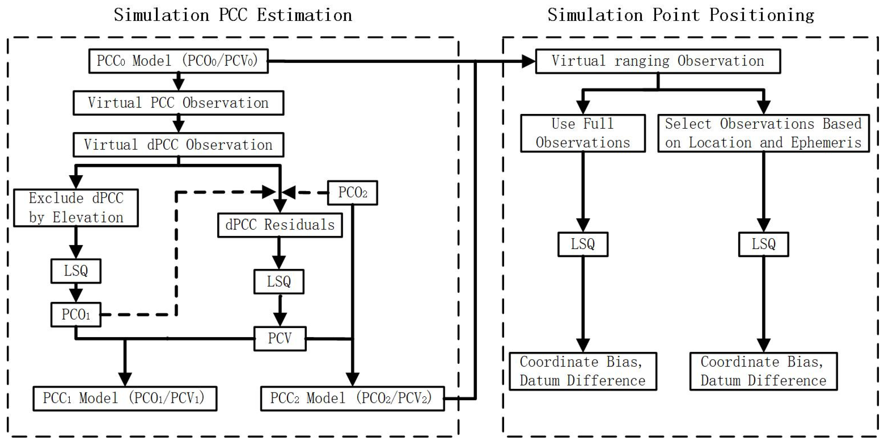
3.1. Simulation of PCC Model Estimation

Based on the existing PCC model from the IGS, a special experiment using virtual observation is designed to simulate the PCC calibration and investigate the factors that might be responsible for different calibrations.

The specially simulated calibration follows two steps. First, we compute virtual PCC and dPCC observations according to Equation (1) from the existing PCC models as will be described in Section 3.1.1. Second, estimation of PCO/PCV is implemented under different strategies, and the estimation process is presented in Section 3.1.2.

3.1.1. Virtual Differenced PCC Observation

In the simulation, a virtual antenna with the model PCC₀(PCO₀/PCV₀) is placed in a north-east-up coordinate system to observe a virtual satellite i with direction (zⁱ, αⁱ), where zⁱ and αⁱ are the zenith and azimuth angles, respectively. The corresponding virtual ranging observation PCC₀ (zⁱ, αⁱ) calculated according to Equation (1) is called the virtual PCC observation. Since the datum B is arbitrary and cannot be determined, differencing between different satellites is performed, which is commonly applied in real field calibration [17,18]. Another virtual satellite j at direction (z^j, α^j) is introduced as a reference. To estimate the PCO/PCV set, the virtual differenced dPCC observation is required and can be obtained as:

$$\begin{array}{ll}dPCC\left({\alpha }^i,z^i\right)& =PC{C}_0\left({\alpha }^i,z^i\right)-PC{C}_0\left({\alpha }^j,z^j\right)\\ & =-PC{O}_0\cdot \left(e^i-e^j\right)+\left[PC{V}_0\left({\alpha }^i,z^i\right)-PC{V}_0\left({\alpha }^j,z^j\right)\right]\end{array}$$

(3)

where e is the line-of-sight vector from the virtual antenna to the virtual satellite. The benefit of using a virtual observation is to avoid irrelevant errors, such as atmospheric delay, clock, multipath, and observation noise, and only the mutual influence imposed by PCO/PCV and their relation are revealed through this experiment.

If the directions of satellite i and j are too close, the elements of (eⁱ − e^j) will be close to 0 and introduce disturbance in the estimation process. To avoid the two signal directions getting too close, two arbitrary reference directions are selected. The first reference satellite is located at (30°, 45°) in zenith and azimuth while the second is (60°, 225°). Virtual observations with zenith angles larger than 45° are differenced with the first reference satellite while those with zenith angles smaller than 45° are differenced with the second reference satellite. Thus, all dPCCs are constructed in this way.

3.1.2. PCO and PCV Estimation

From the virtual dPCC observation in Equation (3), the PCO and PCV parameters are estimated. Since PCO and PCV are both related to the satellite direction, they are highly coupled. Therefore, the estimation is divided into two steps following similar procedures to real field calibration [13,18] to investigate the consistency of different PCO/PCV and its correlation.

When the PCO is estimated, the PCV part is omitted. The vector to be estimated is defined as PCO₁ = (n, e, u), and the three components are the projections of PCO₁ onto the north, east, and up directions, respectively. The coefficient H_i of PCO₁ for the dPCCⁱ is expressed as:

$$\begin{array}{ll}{H}_i=e^i-e^j& =\left\{\mathit{sin}\left(z^i\right)\cdot \mathit{cos}\left({\alpha }^i\right),\mathit{sin}\left(z^i\right)\cdot \mathit{sin}\left({\alpha }^i\right),\mathit{cos}\left(z^i\right)\right\}\\ & -\left\{\mathit{sin}\left(z^j\right)\cdot \mathit{cos}\left({\alpha }^j\right),\mathit{sin}\left(z^j\right)\cdot \mathit{sin}\left({\alpha }^j\right),\mathit{cos}\left(z^j\right)\right\}\end{array}$$

(4)

The spatial hemisphere above the antenna is divided into grids of 5° in zenith by 5° in azimuth, and for each satellite i (i = 1, 2, …, n), the virtual ranging observation dPCCⁱ is calculated at the corresponding grid. Thus, the design matrix H and error vector V are defined as:

$$\{\begin{array}{c}H={\left\{H_0^T,\dots ,H_n^T\right\}}^T\\ V={\left\{dPC{C}_0,\dots ,dPC{C}_n\right\}}^T\end{array}$$

(5)

Moreover, from Equation (5), PCO₁ is obtained with a least-square adjustment (LSQ) as:

$$PC{O}_1={\left(H^T\times H\right)}^{-1}\times \left(H^T\times V\right)$$

(6)

For the PCV estimation, the PCO part in the dPCC observation should be corrected. We substitute the PCO₁ estimated from Equation (6) into Equation (3), and the residuals of dPCC from which the PCV will be extracted are computed as:

$$\begin{array}{ll}Re{s}_i& =dPCC\left({\alpha }^i,z^i\right)+PC{O}_1\cdot \left(e^i-e^j\right)\\ & =\left[PC{V}_0\left({\alpha }^i,z^i\right)-PC{V}_0\left({\alpha }^j,z^j\right)\right]-\left(PC{O}_0-PC{O}_1\right)\cdot \left(e^i-e^j\right)\end{array}$$

(7)

Considering that PCV is a ranging deviation of different directions above the antenna, it is a function of azimuth α and zenith z, which can be appropriately expressed with a set of spherical harmonics (SH) in this estimation. The general form of PCV is expressed as:

$$PCV\left(\alpha ,z\right)={\displaystyle \sum }_{n=0}^{nmax}{\displaystyle \sum }_{m=0}^n\left(C_{n,m}\cdot \mathit{cos}m\alpha +S_{n,m}\cdot \mathit{sin}m\alpha \right)\cdot P_{n,m}\left(\mathit{cos}z\right)$$

(8)

where C_n,m and S_n,m are the corresponding spherical harmonics that need to be estimated, n and m are the order and degree of the spherical harmonics that meet the condition of $m\le n$, and $P_{n,m}$ is the Legendre polynomials. Similar to the practice of real PCC calibration, spherical harmonics of order 8 and degree 8 are used in this experiment.

To avoid rank deficiency of the normal equation, a special tight constraint of zero PCV in the zenith direction is applied as:

$$PCV\left(0,\alpha \right)={{\displaystyle \sum }}_{n=0}^{nmax}{C}_{n,0}·P_{n,0}\left(1\right)=0$$

(9)

With a similar LSQ process for PCO estimation, the coefficients C_n,m and S_n,m can be obtained, and then the PCV at any direction can be calculated according to the spherical harmonics. Thus, PCV₁ is obtained together with PCO₁, and a new antenna model PCC₁(PCO₁/PCV₁) is therefore estimated from the dPCC observation constructed by PCC₀(PCO₀/PCV₀).

It should be noted that if any other set of PCO₂ is introduced in Equation (7), a corresponding PCV₂ will be obtained and lead to the antenna model PCC₂(PCO₂/PCV₂). Therefore, we will intentionally adjust the PCO₂ in the estimation of PCV, and investigate the correlation between the variation in PCO and PCV.

3.2. Simulation of Point Positioning

As described in Section 3.1, the antenna model PCC obtained from the simulation estimation is obviously different in numerical values in terms of PCO or PCV compared with the original model if a different PCO is introduced in the PCV estimation. We want to investigate the consistency of these different PCC models on positioning. Therefore, a simulated point positioning is designed.

Given two antenna models PCC₀ and PCC₁ with certain differences in PCO and PCV, we assume an antenna with PCC₁ is placed in the north-east-up coordinate system to track the signal from a virtual satellite i with zenith zⁱ and azimuth αⁱ, and the virtual ranging observation is PCC₀; thus, the equation of the virtual ranging observation Vⁱ is written as:

$$V^i=PC{C}_0^i\left(\alpha , z\right)-PC{C}_1^i\left(\alpha , z\right)=-e\cdot \left[dn,de,du\right]-\nabla B$$

(10)

Here, the parameters to be estimated are denoted as X = (dn, de, du, $\nabla B$), specifically the coordinate biases (dn, de, du) along with the datum difference $\nabla B$. The coefficient H_i of X for Vⁱ is written as:

$$H_i=\left[-e,-1\right]=\left[-\mathit{sin}\left(z\right)\cdot \mathit{cos}\left(\alpha \right),-\mathit{sin}\left(z\right)\cdot \mathit{sin}\left(\alpha \right),-\mathit{cos}\left(z\right),-1\right]$$

(11)

If more than four satellites are observed, X can be estimated. Therefore, more virtual satellites are distributed at different directions in the upper hemisphere. The design matrix H and error vector V for all virtual ranging observations of satellites in the point position experiment are obtained as:

$$\{\begin{array}{c}H={\left[H_1^T,\dots ,H_n^T\right]}^T\\ V={\left[V_1,\dots ,V_n\right]}^T\end{array}$$

(12)

Finally, the coordinate biases are obtained through a least-square adjustment process as:

$$X={\left(H^T\times H\right)}^{-1}\times \left(H^T\times V\right)$$

(13)

Coordinates biases estimated in this virtual point positioning simulation can be viewed as an indicator of the differences in PCC₀ and PCC₁ in the coordinate domain.

4. Coupling Analysis of PCO and PCV Parameters

To validate and compare the mutual influence between PCO and PCV in the calibration, several types of experiments are designed and implemented as described in Section 3. The original PCC models are based on igs05.atx, igs08.atx, igs14.atx, and igsR3.atx released by IGS (https://files.igs.org/pub/station/general/, accessed on 18 January 2022). In addition, absolute antenna calibration was implemented at Wuhan University [18], and multi-GNSS PCC model calibration is currently under testing. Benefiting from previous work, the impact of PCO and PCV on calibration can be investigated through field GNSS data. Particularly, in this contribution, the field calibration data for TRM59800.00 NONE were collected on DoY (Day of Year) 332 in 2020, and the timespan was 24 h.

4.1. PCO Estimation by Different Elevation Masks

The estimates of PCO₁ will be precisely equal to PCO₀ if dPCC observations are constructed from PCC(PCO₀/PCV₀), where PCV₀ are all zero. However, the PCV parts are non-zero and will cause differences in the PCO estimates. In the real data processing of field calibration, as different elevation masks are applied, the dPCC observations containing different PCVs are changed in the PCO estimation. Therefore, PCO estimates might vary as different elevation masks are applied. In this virtual simulation experiment, we set an elevation mask to control the computation of the virtual dPCC observation and investigate the differences in the PCO estimates as a function of the elevation mask.

Following the steps described in Section 3.1, the PCO estimates of antenna TRM59800.00 NONE from the virtual dPCC observation are analyzed as a detailed example shown in the left panel of Figure 5 while the right panel shows the real calibration in the field. The trends for the simulated estimation and field calibration are similar. As the elevation mask angle increases, biases change slowly in the north and east components but decrease sharply in the up component. The field calibration curve is smoother than that of the simulated estimation. PCO estimation in the up component is apparently more vulnerable and sensitive to the elevation cutoff angle than the other two components. In the simulation estimation, since there is no other error or noise in the virtual dPCC observation, the biases must be caused by the only disturbance of PCV that is ignored in the process. In both the simulation estimation and field calibration, the PCO biases with L1 varies more significantly than those with L2, which coincides with the fact that the absolute PCV value for L1 is larger than that for L2. It can be concluded that the variation in PCO biases is highly dependent on the PCV magnitude.

Furthermore, we performed the PCO estimation for all PCC models presented in igs14.atx and set the elevation mask as zero degrees. Differences exceeding 1 mm in the up component of PCO estimates of approximately 140 antennas are shown in Figure 6. Except for several types, the estimates of the up components for most of the antennas are larger than their original values and can reach 3~6 mm. However, the precision of field PCO estimation can reach the 1 mm level or even better than 0.5 mm. In this simulation estimation, the PCO estimates might not be equal to the values used to construct the virtual dPCC observation, although only the PCC without any external error is induced in the simulation. It suggests that the PCC calibration might lead to different PCO estimates due to different process strategies, which indicate a low stability for different calibration strategies. The neglecting or partial selection of dPCC observations can cause a significant disturbance in the PCO estimates.

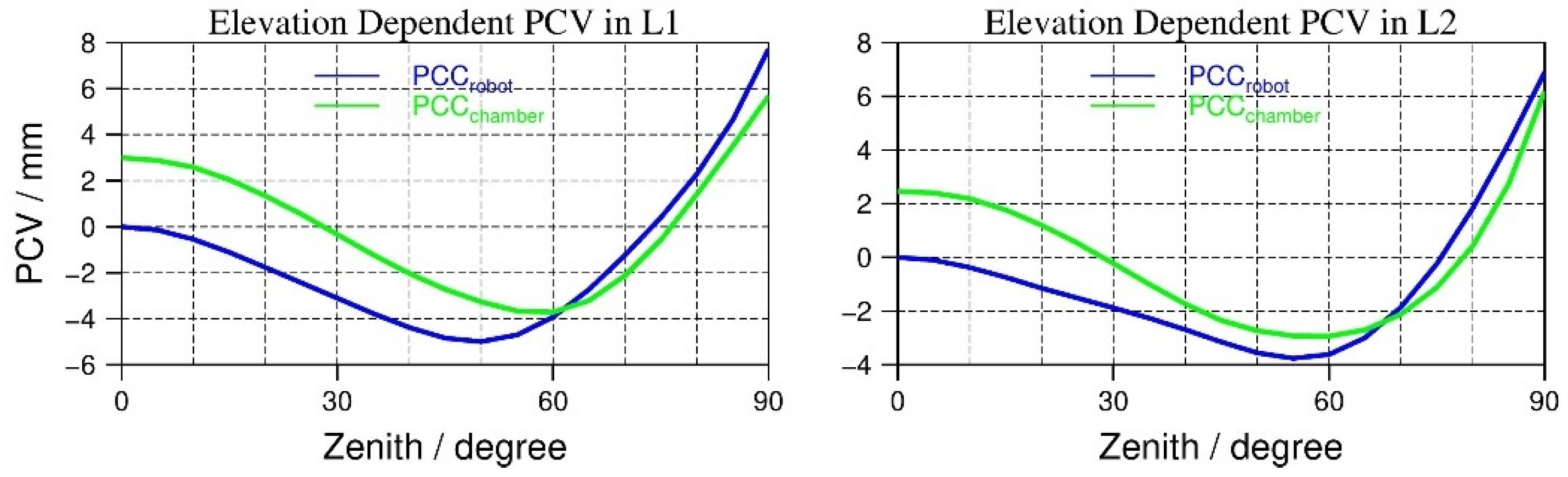
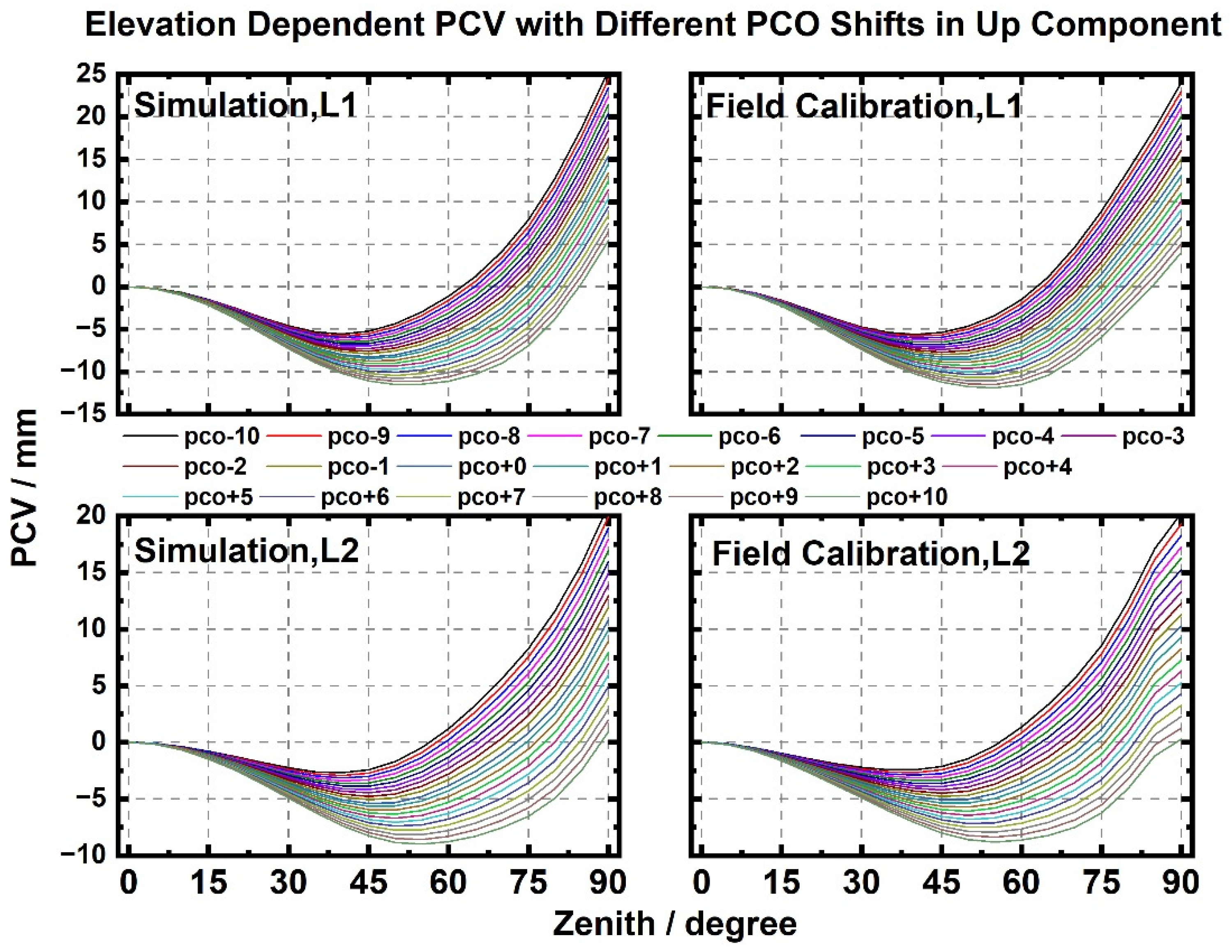
4.2. Coupling of PCO Shifts and PCV Variation

According to the discussion in the previous section, the estimated PCO will be affected while PCV is ignored in the dPCC observation. Since the estimated PCO is introduced into the dPCC observation to compute residuals for the estimation of PCV, different PCOs might lead to different PCV estimations. The relation between variations in PCO and PCV will be analyzed.

Since the PCO is dominant in the up component, several intentional shifts were added to the up component of the original PCO value in this experiment and introduced back into the estimation of PCV. Comparison was made between the PCV estimates afterward. Following the steps described in Section 3.1, we performed the PCV estimation of antenna TRM59800.00 and the original model PCC₀ in igs14.atx is used in this experiment. Specifically, shifts from −10 to 10 mm with an interval of 1 mm are added to the up component of PCO₀ to obtain PCO_s, and PCO_s is then introduced into the computation of dPCC residuals. The elevation-dependent PCV estimation is shown in the left column of Figure 7 while the PCV estimation from field calibration is placed in the right column.

The elevation-dependent PCV curves are nearly the same for the simulation estimation and field calibration. It can be clearly seen that the variations in the elevation-dependent PCV curves with different PCO shifts s are similar. All curves start from zero in the zenith direction due to the tight constraint of zero PCV in the zenith direction. As the zenith increases, the curves diverge from each other, and the width of the spacing expands. At a certain zenith, the PCV value increases as the intentional shift decreases, and all PCV values are evenly spaced. When the zenith angle reaches 90 degrees, the distances between adjacent curves are all 1 mm, which is precisely the interval of the intentional shifts. From the apparent negative correlation between the PCO shift and PCV value, it can be safely assumed that the PCO shifts can be perfectly compensated by the PCV estimates. In this sense, only if the dPCC observation is correct or consistent can the separation of PCC lead to several equivalent PCO/PCV sets even with a large numerical difference in individual PCO or PCV values.

In fact, the relation between the PCO shift and the PCV value can be deduced theoretically according to [19], and the transformation from one PCC₁(PCO₁/PCV₁) to another PCC₂(PCO₂/PCV₂) with d_pco = PCO₂ − PCO₁ = (d_N, d_E, d_U) is based on Equation (1) as:

$$\begin{array}{ll}PCC\left(\alpha ,z\right)& =-PC{O}_1\cdot e+PC{V}_1\left(\alpha ,z\right)+B_1\\ & =-\left(PC{O}_2-d_{pco}\right)\cdot e+PC{V}_1\left(\alpha ,z\right)+B_1\\ & =-PC{O}_2\cdot e+\left[PC{V}_1\left(\alpha ,z\right)+d_{pco}\cdot e+d_B\right]+\left(B_1-d_B\right)\\ & =-PC{O}_2\cdot e+PC{V}_2\left(\alpha ,z\right)+B_2\end{array}$$

(14)

Therefore,

$$\{\begin{array}{cc}\hfill PC{V}_2\left(\alpha ,z\right)& =PC{V}_1\left(\alpha ,z\right)+d_{pco}\cdot e+d_B\hfill \\ \hfill B_2& =B_1-d_B\hfill \end{array}$$

(15)

To conform with the convention of $PC{V}_1\left(\alpha ,0\right)=PC{V}_2\left(\alpha ,0\right)=0$,

$$\begin{array}{ll}PC{V}_2\left(\alpha ,0\right)& =PC{V}_1\left(\alpha ,0\right)+d_{pco}\cdot e+d_B\\ & =0+\left(d_N,d_E,d_U\right)\cdot \left(e_N,e_E,e_U\right)+d_B\\ & =\left(d_N,d_E,d_U\right)\cdot \left(\sin 0\cos \alpha ,\sin 0\sin \alpha ,\cos 0\right)+d_B\\ & =d_U+d_B=0\end{array}$$

(16)

This condition leads to:

$$d_B=-d_U$$

(17)

and,

$$PC{V}_2\left(\alpha ,z\right)=PC{V}_1\left(\alpha ,z\right)+d_{pco}\cdot e-d_U$$

(18)

Particularly, if a shift $d_U$ is added to the upper component of PCO, i.e., $d_{pco}=\left(0,0,d_U\right)$, a simplified relation between $PC{V}_1$ and $PC{V}_2$ is obtained as:

$$PC{V}_2\left(\alpha ,z\right)=PC{V}_1\left(\alpha ,z\right)-d_U\cdot \left(1-\mathit{cos}\left(z\right)\right)$$

(19)

Regarding the shift $d_N$ or $d_E$, they will not influence the average PCV at a certain zenith since:

$$\{\begin{array}{c}{{\displaystyle \int }}_0^{2\pi }\left(d_N\cdot \mathit{sin}z\mathit{cos}\alpha \right)d\alpha =0\\ {{\displaystyle \int }}_0^{2\pi }\left(d_E\cdot \mathit{sin}z\mathit{sin}\alpha \right)d\alpha =0\end{array}$$

(20)

However, it will obviously affect the PCV value at the same zenith, and whether it is amplified or reduced will depend on $d_N$, $d_E$ and the original PCV value.

Considering the extreme example JAV_RINGANT_G3T NONE mentioned in Section 2.2, this transformation is applied and the differences will be investigated. The anechoic chamber calibration from igsR3.atx is denoted as PCC₁(PCO₁/PCV₁) while robot calibration from igs14.atx is denoted as PCC₂(PCO₂/PCV₂). To align PCC₁ to PCC₂ with the same PCO₂, several operations were performed and L1 was taken as an example. First, the difference in datum B of 3 mm is subtracted from all the PCV of PCC₁ to obtain PCC₃(PCO₁/PCV₃). PCV₃ follows the convention of zero PCV at a zero zenith angle, and is equivalent to PCC₁ in terms of positioning. The 3 mm datum differences can be absorbed into the clock or ambiguity. Second, we add d_pco to PCO₁ and correct the PCV₃ value at each grid point according to Equation (18) to obtain PCC₄(PCO₂/PCV₄) while d_pco is the differences between PCO₁ and PCO₂. Here, in this case, d_pco for L1 is (−0.21 mm, 0.05 mm, −6.02 mm) as listed in Table 1. Finally, the same PCO₂ is set for robot calibration PCC₂(PCO₂/PCV₂) and transformed anechoic chamber calibration PCC₄(PCO₂/PCV₄). PCV₂ and PCV₄ can be directly differenced and compared with common PCO₂. The procedures of this alignment are shown in Figure 8, and the differences in robot calibration and anechoic chamber calibration before and after the alignment for JAV_RINGANT_G3T NONE are presented in Figure 9.

As can be seen in Figure 9, obvious numerical differences exceeding 3 mm in PCV between PCC₁ and PCC₂ can be found for both L1 and L2. After the operations described before, PCC₁ is aligned to PCC₂ with the same PCO₂, and differences in PCV are dramatically decreased to approximately 1 mm except for some areas with low elevation. This case can be an example to validate the equivalence of PCC models with large numerical differences in PCO/PCV and the correctness of the alignment methods. Therefore, PCC models with large numerical differences can still be approximately equivalent models if the alignment procedures decrease the differences to a 1 mm level. This practice can provide an approach to compare the PCV with PCO aligned rather than comparing PCO and PCV separately, and it can avoid false judgment caused by a direct discrepancy in PCO or PCV, and reveal the overall differences with consideration of both PCO and PCV combined.

5. Impact of Equivalent PCC Models on Positioning

Although biases of magnitude up to the millimeter or even centimeter level may exist in PCC models from different institutions due to different calibration conditions and strategies, the differences may be decreased if aligning their PCO to a common value. The comprehensive impact of these equivalent PCC models on positioning needs further investigation.

5.1. Virtual Positioning Biases with Equivalent PCC Models

Following the steps described in Section 3.2, we performed the simulated positioning experiments based on the original PCC₀ model of TRM59800.00 NONE in igs14.atx, and a sets of equivalent PCC_s models are obtained according to Equation (18) with d_pco = (0, 0, s) mm, s denotes the differences of PCO in the up component between PCC₀ and PCC_s, and in this experiment, s is from −10 to 10 mm with an interval of 1 mm. In addition, the virtual satellites are located in the 1° by 1° grid of the antenna upper hemisphere, and PCC differences from all directions are included in the point positioning. As is described in Section 3.2, position biases in the north, east, and up components along with datum difference $\nabla B$ are estimated and shown in Figure 10. Positioning bias in the up component is all less than 0.01 mm with a different shift s in the PCO up component for L1 and L2 signals; additionally, the biases in the north and east are almost zero within the truncation precision of 10⁻⁵ mm, which is unperceivable or ignored in positioning. It is found that coordinate biases remain quite steady as different PCC_s is applied and even the differences s reach 10 mm. Overall, positioning biases caused by equivalent PCO/PCV sets with centimeter-level differences remain at the 0.01 mm level, which is insignificant for most phase-based applications. The datum difference $\nabla B$ is highly correlated with the intentional shift s. In the actual GNSS application, the coefficient of the datum difference $\nabla B$ is the same as the receiver clock or ambiguity, and $\nabla B$ was obviously absorbed into the clock and ambiguity parameter or eliminated by differencing observations between satellites. In addition, the position biases in this virtual point positioning can be used to measure the difference of the two PCC models in the coordinated domain, which is a convenient way of comparing PCV in the whole grid cells.

Based on this experiment, we can conclude that insignificant influences are imposed on the positioning estimate if equivalent PCC models, even with differences at the centimeter level, are applied. Therefore, consistency can be ensured for these PCC models, and it is appropriate to use or replace them without the extra worry of significant PCC biases.

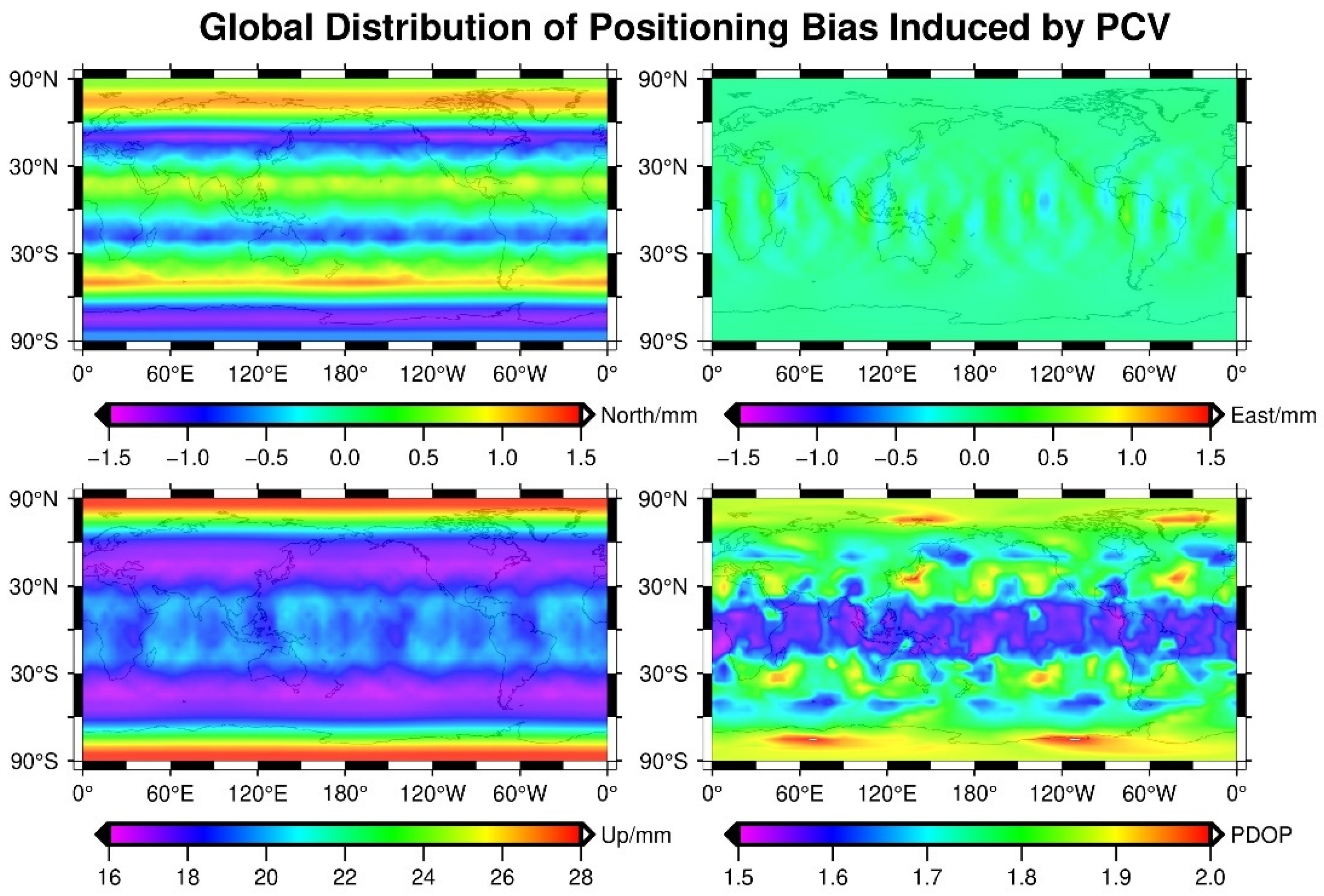
5.2. Distribution of Virtual Positioning Biases

In the actual scenarios, it is impossible for a single receiver to track satellites from all directions, and the PCCs are usually sparse and unevenly distributed. Therefore, the impact of PCC on position may vary with the user’s location. Researchers have proposed a latitude-dependent model to correct such a position offset [20,21], and it is necessary to investigate the differences in the equivalent PCC models on positioning in such circumstances. We chose DoY 070 in 2021 as an example and collected the GPS ephemeris and set a virtual station at different locations across global areas, and satellite positions were computed according to the real ephemeris in a timespan from 0:00 to 24:00. Afterward, the virtual ranging observations were calculated if the satellite was above the horizon line, and positioning experiments were performed according to Section 3.2. Here, the station is placed on every grid cell from −180 to 180 degrees in longitude and −85 to 85 degrees in latitude with an interval of 5 degrees. The sampling rate of the satellite position is set to 1 min. In this simulation experiment, we chose the models for L1 of TRM59800.00 NONE in igs14.atx as PCC₀.

We first investigated the impact of PCV variation on positioning according to Section 3.2. Here, the virtual ranging observation is constructed by PCC₀(PCO₀/PCV₀) and PCC₁(PCO₁/PCV₁). PCO₁ is equal to PCO₀ and PCV₁ is zero. Therefore, only the PCV₀ is left in the virtual ranging observations and the position biases reflect the impact of PCV on the positioning at different locations. The distributions of the positioning biases in the north, east, and up components along with the position dilution of precision (PDOP) are shown in Figure 11. The positioning biases induced only by PCV are not evenly distributed, and the biases in the north and up components are significantly correlated with the latitude. A weaker correlation can be found between bias in the east component with the longitude. The 95th percentile of the PDOP was calculated over one week, and the distribution of the PDOP is also latitude dependent but not the same as the position biases, which means that the variation in the PCC contributes to the positioning biases. For the magnitude, bias from 16~28 mm in the up component contributes to most of the positioning error budget, which is reasonable for a large variation range of PCV with zenith and a small range with azimuth. Furthermore, biases, especially in the up component, will increase to the decimeter level if PCO₁ is set to zero. However, the biases induced by the PCO at different locations are the same since the PCO can be viewed as constant shifts in the local north-east-up coordinates. It should be noted that the positioning bias distributions are not fixed in Figure 11 and will change if different PCC models or constellations are applied in this simulated experiment. In a word, the influence of PCC on positioning cannot be ignored in high-precision applications, and should be corrected with accurate PCC models.

Next, we construct an equivalent PCC₂(PCO₂/PCV₂) model with d_pco = (0, 0, −10) mm between PCO₀ and PCO₂, and PCV₂ is obtained by transformation of PCV₀ according to Equation (18). Moreover, the simulated point positioning is performed using PCC₀ and PCC₂. Finally, the distributions of the positioning biases between PCC₀ and PCC₂ are shown in Figure 12.

It can be clearly seen that positioning biases are dramatically decreased to the 0.01 mm level, which is acceptable for normal GNSS applications. Additionally, the significantly uneven distribution of positioning biases disappears, which shows a high consistency between the equivalent PCC₂ model and original PCC₀ model at different location. In particular, the distribution of the datum difference $\nabla B$ between the two PCC models is negatively correlated with biases in the upper component, and the −10 mm difference is perfectly absorbed into $\nabla B$ rather than the coordinates, which is the same as the clock parameter in field data positioning. This example can validate the self-consistency of the equivalent PCC models. Therefore, it can be safely concluded that almost no positioning biases are induced if an equivalent PCC model is applied, even if large numerical differences might exist between them. The same positioning investigations with the equivalent PCC model were performed on the other PCC models available in igs14.atx, and the results of the simulated point positioning biases show high consistency.

5.3. Positioning Validation

For antenna JAV_RINGANT_G3T NONE, simulation positioning experiments of the PCC models from robot calibration in igs14.atx and anechoic chamber calibration from igsR3.atx are performed, and the biases in L1 and L2 are listed in

Table 2. Biases in the PCC model for JAV_RINGANT_G3T NONE between robot calibration and anechoic chamber calibration in simulated positioning (unit:mm).

Bias	N	E	U
L1	−0.16	0.09	−0.55
L2	0.51	−0.35	0.13

. The biases in the simulated positioning are all within 1 mm in the north, east, and up component, which is obviously smaller than the direct numerical differences in the PCC models.

Apart from the simulated positioning experiments, static PPP and baseline solution are performed to validate the simulated positioning experiment and consistency of the PCC model for antenna JAV_RINGANT_G3T NONE. In this case, static field GNSS data from two IGS station BIK0 and POL2 are collected from DoY 071 to 077 in 2021, and station BIK0 is equipped with antenna JAV_RINGANT_G3T NONE whose PCC model was analyzed in the previous discussion. For this special antenna, the PCC model from robot calibration is chosen from igs14.atx with anechoic chamber calibration from igsR3.atx. In the data processing, the two PCC models will be applied, respectively, and the differences in the coordinate series will be analyzed to investigate the consistency of the two PCC models.

At first, the typical PPP solution is performed for station BIK0 using ionosphere-free (IF) combination of L1/L2, and the PCC model from robot and anechoic chamber calibration are applied, respectively. The root mean square (RMS) of the differences in the coordinate series are listed in

Table 3. RMS of baseline and PPP solution differences between the PCC model from robot and chamber calibration (unit:mm).

DoY	PPP Solution			Baseline Solution
	IF			L1			L2
	Horizon	Up	3D	Horizon	Up	3D	Horizon	Up	3D
071	1.27	3.51	3.74	0.15	0.13	0.21	0.60	0.63	0.88
072	1.28	3.53	3.77	0.11	0.10	0.17	0.58	0.34	0.71
073	1.28	3.50	3.74	0.12	0.14	0.20	0.61	0.41	0.74
074	1.28	3.51	3.75	0.30	0.35	0.48	0.95	0.51	1.15
075	1.28	3.49	3.73	0.16	0.15	0.23	0.63	0.32	0.72
076	1.28	3.52	3.75	0.13	0.06	0.16	0.56	0.47	0.74
077	1.29	3.37	3.61	0.13	0.13	0.20	0.59	0.40	0.72
mean	1.28	3.49	3.73	0.16	0.15	0.24	0.65	0.44	0.81

. The average RMS of the PPP solution differences are 1.28, 3.49, and 3.73 mm in the horizon, up, and 3D component. It can be easily seen that the RMS is smaller than the direct numerical differences in the original PCO/PCV sets listed in Table 1, where differences for a single frequency can reach −6.02 mm in L1 and −3.86 mm in L2. However, the difference in the PPP solution is larger than the simulated point positioning biases listed in Table 3. This might be caused by the IF observation, and the difference for the IF observation should be amplified by the differences in L1 and L2 combined.

Furthermore, the single frequency baseline solution of BIK0−POL2 is performed to investigate the consistency of the two PCC models. The baseline positioning was conducted through a forward Kalman filter with double-differencing observation. The coordinate differences series of the baseline positioning by applying different PCC models at DoY 071, 2021 are shown in Figure 13. For L1, the differences in the coordinates between the two PCC models are quite small and stable. The magnitudes of the positioning differences in the north, east, and up components are all less than 1 mm. However, the numerical PCO differences in the two models between robot and chamber calibration can exceed 6 mm, as presented in Table 1. The PCV differences can reach 3 or 4 mm in certain directions, as shown in Figure 9. Although larger differences and variations can be found for L2 compared with L1, the magnitudes remain within 1 mm. This phenomenon is consistent with the result shown in Figure 9. After PCO is aligned with the same values, the PCV differences are still larger with L2 than with L1. In other words, the numerical differences in the PCC model up to 6 mm are seldomly embodied in the positioning estimation. The effect of the PCO differences might be canceled out by the PCV differences if equivalent PCC models are applied.

To further investigate and validate the previous conclusion, the baseline solution of BIK0−POL2 was performed for 7 days, and the RMS of the coordinate differences in the horizon, up, and 3D components using the PCC model from robot and chamber calibration are calculated and listed in Table 3. For L1, the differences induced by the PCC model are all less than 0.5 mm, while the counterparts for L2 are slightly larger, ranging from 0.72 to 1.15 mm. In terms of the average RMS over 7 days, differences of 0.16, 0.15, and 0.52 mm in the horizon, up, and 3D component in L1 were observed and 0.65, 0.44, and 0.81 mm for L2. The comparison of the baseline solution with the two PCC models with large numerical differences in PCO and PCV showed a comparably smaller impact on coordinate estimation. In addition, the coordinate difference in the baseline solution is more consistent with the simulated point positioning result in Table 2 than that in the PPP solution, which indicates the advantages of the baseline solution over the PPP solution in PCC validation.

Based on the simulation analysis and field data positioning, we can conclude that for a certain antenna, its PCC model could be presented in several sets of PCOs and PCVs. Even if large numerical differences may exist, these different PCC models can still be viewed as equivalent or approximately equivalent.

6. Conclusions

In this contribution, we analyzed the factors that may be responsible for large numerical differences in existing PCC models and investigated the mutual impact of PCO and PCV in calibration and positioning through simulation and field experiments. The main conclusions based on these experiments are as follows.

Numerical differences at the sub-centimeter level in PCO or PCV exist for some PCC models by comparing them between different versions of ANTEX files. However, the magnitude of these differences is apparently larger than the calibration precision of 1.0 or even 0.5 mm.

The simulation and field experiments showed that the PCO and PCV are highly coupled with each other in calibration. First, omitting PCV in PCO estimation disturbs the PCO estimates, and the disturbance in PCO forwardly affects the PCV extraction. Thus, different strategies in calibration might lead to different PCO/PCV sets, and it explains the PCC differences from different institutions. In the virtual estimation of PCO, the elevation mask was chosen to decide what range of PCV will be included in the PCO estimation, and the result shows that the up component of the PCO estimates will vary beyond 10 mm if the elevation mask is set from 0 to 30 degrees. In the simulated estimation of PCV, several intentional shifts were added to the original PCO value. The estimated PCV values show synchronized variation with the shifts in PCO and will perfectly compensate for the shifts. Therefore, a specific PCC model can be expressed in multiple PCO/PCV sets in calibration if different strategies are applied, and these PCC models are indeed equivalent.

Then, we investigated the impact of PCC on positioning and the applicability of an equivalent PCC model. Considering the actual constellation, positioning biases induced in PCV are related to latitude or longitude. The variation in position biases is correlated with the magnitude of the PCV. However, these positioning biases decrease to the 0.01 mm level if an equivalent PCC model is applied. The results of the positioning experiments can prove that these different PCC models with large numerical differences in PCO/PCV for one antenna are equivalent in positioning.

In this contribution, an extra constant datum parameter B in the PCC model in addition to the classical PCO/PCV set was applied. With the help of parameter B, one set of PCC can be transformed to another equivalent set with certain numerical differences in PCO and PCV while their consistency in positioning remains after the PCC transformation. An extreme case of antenna JAV_RINGANT_G3T NONE was investigated in detail. For this antenna, its PCC models by robot and anechoic chamber calibration are presented in igs14.atx and igsR3.atx, respectively, while their numerical differences can reach 6 mm. However, the differences dramatically decrease to the 1 mm level after following the alignment procedures, which means that the two PCC models are approximately equivalent. Comparing the two PCC models using the simulated point positioning described in this contribution, the differences in the coordinate domain are (−0.16, 0.09, −0.55) mm for L1 and (0.51, −0.35, 0.13) mm for L2 in the north, east, and up component, which is apparently smaller. In a positioning experiment with field GNSS observation, the coordinate differences induced just by the two PCC models are also less than 1 mm in the. baseline solution and 4 mm in the PPP solution. The better consistency in the baseline solutions might be explained by the single frequency observation, since the ionosphere-free combination is used in the PPP solution. The comparison of simulation and field positioning can validate the correctness of the constant datum parameter B and the alignment procedures.

Based on the work in this contribution, we hope to provide a new vision to understand the PCC model and provide a comprehensive method to evaluate its impact on calibration and positioning.

References

1. Tranquilla, J.M.; Colpitts, B.G. GPS Antenna Design Characteristics for High-Precision Applications. J. Surv. Eng. 1989, 115, 2–14. [Google Scholar] [CrossRef]
2. Rocken, C.; Meertens, C.; Stephens, B.; Braun, J.; VanHove, T.; Perry, S.; Ruud, O.; McCallum, M.; Richardson, J. UNAVCO Academic Research Infrastructure (ARI) Receiver and Antenna Test Report. UNAVCO Boulder Facility International Report. Available online: https://www.unavco.org/projects/project-support/development-testing/publications/ari_test.pdf (accessed on 18 January 2022).
3. Schupler, B.R.; Clark, T.A.; Allshouse, R.L. Characterizations of GPS user antennas: Reanalysis and new results. In GPS Trends in Precise Terrestrial, Airborne, and Spaceborne Applications; Springer: Berlin/Heidelberg, Germany, 1996; pp. 328–332. [Google Scholar]
4. Mader, G.L. GPS Antenna Calibration at the National Geodetic Survey. GPS Solut. 1999, 3, 50–58. [Google Scholar] [CrossRef]
5. Wübbena, G.; Schmitz, M.; Menge, F.; Seeber, G.; VÖLKSEN, C. A new approach for field calibration of absolute GPS antenna phase center variations. Navigation 1997, 44, 247–255. [Google Scholar] [CrossRef]
6. Menge, F.; Seeber, G.; Volksen, C.; Wübbena, G.; Schmitz, M. Results of absolute field calibration of GPS antenna PCV. In Proceedings of the 11th International Technical Meeting of the Satellite Division of The Institute of Navigation (ION GPS 1998), Nashville, TN, USA, 15–18 September 1998. [Google Scholar]
7. Bergstrand, S.; Jarlemark, P.; Herbertsson, M. Quantifying errors in GNSS antenna calibrations. J. Geod. 2020, 94, 105. [Google Scholar] [CrossRef]
8. Krzan, G.; Dawidowicz, K.; Wielgosz, P. Antenna phase center correction differences from robot and chamber calibrations: The case study LEIAR25. GPS Solut. 2020, 24, 747. [Google Scholar] [CrossRef] [Green Version]
9. Darugna, F.; Wübbena, J.B.; Wübbena, G.; Schmitz, M.; Schön, S.; Warneke, A. Impact of robot antenna calibration on dual-frequency smartphone-based high-accuracy positioning: A case study using the Huawei Mate20X. GPS Solut. 2021, 25, 2621. [Google Scholar] [CrossRef]
10. Villiger, A.; Dach, R.; Schaer, S.; Prange, L.; Zimmermann, F.; Kuhlmann, H.; Wübbena, G.; Schmitz, M.; Beutler, G.; Jäggi, A. GNSS scale determination using calibrated receiver and Galileo satellite antenna patterns. J. Geod. 2020, 94, 6109. [Google Scholar] [CrossRef]
11. Geiger, A. Modeling of phase center variation and its influence on GPS-positioning. In GPS-Techniques Applied to Geodesy and Surveying; Groten, E., Strauß, R., Eds.; Springer: Berlin Heidelberg, Germany, 1988; pp. 210–222. ISBN 978-3-540-45962-0. [Google Scholar]
12. Wübbena, G.; Schmitz, M.; Menge, F.; Böder, V.; Seeber, G. Automated absolute field calibration of GPS antennas in real-time. In Proceedings of the International Technical Meeting, ION GPS-00, Salt Lake City, UT, USA, 19–23 September 2000. [Google Scholar]
13. Bilich, A.; Mader, G.L. GNSS absolute antenna calibration at the national geodetic survey. In Proceedings of the 23rd International Technical Meeting of The Satellite Division on the Institute of Navigation, Portland, OR, USA, 1–24 September 2010; pp. 1369–1377. [Google Scholar]
14. Kröger, J.; Kersten, T.; Breva, Y.; Schön, S. Multi-frequency multi-GNSS receiver antenna calibration at IfE: Concept-calibration results-validation. Adv. Space Res. 2021, 68, 4932–4947. [Google Scholar] [CrossRef]
15. Riddell, A.; Moore, M.; Hu, G. Geoscience Australia’s GNSS antenna calibration facility: Initial results. In Proceedings of the IGNSS Symposium 2015 (IGNSS2015), Gold Coast, Australia, 14–16 July 2015. [Google Scholar]
16. Rothacher, M.; Schmid, R. ANTEX: The Antenna Exchange Format, Version 1.4; 15 September 2010. Available online: https://files.igs.org/pub/station/general/antex14.txt (accessed on 18 January 2022).
17. Willi, D.; Koch, D.; Meindl, M.; Rothacher, M. Absolute GNSS Antenna Phase Center Calibration with a Robot. In Proceedings of the 31st International Technical Meeting of The Satellite Division of the Institute of Navigation (ION GNSS+ 2018), Miami, FL, USA, 24–28 September 2018; pp. 3909–3926. [Google Scholar]
18. Hu, Z.; Zhao, Q.; Chen, G.; Wang, G.; Dai, Z.; Li, T. First Results of Field Absolute Calibration of the GPS Receiver Antenna at Wuhan University. Sensors 2015, 15, 28717–28731. [Google Scholar] [CrossRef] [PubMed] [Green Version]
19. Schön, S.; Kersten, T. Comparing Antenna Phase Center Corrections: Challenges, Concepts and Perspectives. In Proceedings of the IGS Analysis Workshop, Pasadena, CA, USA, 23–27 June 2014. [Google Scholar]
20. Baire, Q.; Bruyninx, C.; Legrand, J.; Pottiaux, E.; Aerts, W.; Defraigne, P.; Bergeot, N.; Chevalier, J.M. Influence of different GPS receiver antenna calibration models on geodetic positioning. GPS Solut. 2014, 18, 529–539. [Google Scholar] [CrossRef]
21. Rebischung, P.; Griffiths, J.; Ray, J.; Schmid, R.; Collilieux, X.; Garayt, B. IGS08: The IGS realization of ITRF2008. GPS Solut. 2012, 16, 483–494. [Google Scholar] [CrossRef]
Figure 1. Antenna phase center correction model. PCO is a vector pointing from antenna reference point (ARP) to mean phase center while PCV is the range variation based on PCO; B denotes the datum; e denotes the directional vector from antenna to satellite.
Remotesensing 14 00540 g001
Figure 2. Differences in PCO for different PCC models in different ANTEX versions.
Remotesensing 14 00540 g002
Figure 3. Difference in the elevation-dependent PCV for JAV_RINGANT_G3T NONE between robot calibration (from igs14.atx) and anechoic chamber calibration (from igsR3.atx).
Remotesensing 14 00540 g003
Figure 4. Design of the simulation experiment for PCC estimation and point positioning.
Remotesensing 14 00540 g004
Figure 5. Difference between PCO estimates and the original value in igs14.atx for L1/L2 as a function of different elevation masks.
Remotesensing 14 00540 g005
Figure 6. Differences in the up component of PCO estimates compared with its original value for antennas in igs14.atx.
Remotesensing 14 00540 g006
Figure 7. PCV curve variation with different PCO bias in the up component.
Remotesensing 14 00540 g007
Figure 8. Procedures of aligning the PCC model of anechoic chamber and robot calibration with the same PCO for antenna JAV_RINGANT_G3T NONE.
Remotesensing 14 00540 g008
Figure 9. Differences in the PCC model between robot and chamber calibration for antenna JAV_RINGANT_G3T NONE before and after alignment. PCV1 and PCV4 are from the anechoic chamber calibration before and after PCO aligned to the same as robot calibration, PCV2 is from the robot calibration.
Remotesensing 14 00540 g009
Figure 10. Position biases of different PCCs models with shifted PCO and PCV combinations.
Remotesensing 14 00540 g010
Figure 11. Global distribution of positioning biases induced from PCV for TRM59800 in L1.
Remotesensing 14 00540 g011
Figure 12. Distribution of simulated positioning biases between equivalent PCC models for antenna TRM59800.00, L1.
Remotesensing 14 00540 g012
Figure 13. Differences in the north, east, and up component of baseline positioning between IGS Station POL2 and BIK0 with the PCC model from robot and chamber calibration.
Remotesensing 14 00540 g013