
Reflective Noise Filtering of Large-Scale Point Cloud Using Transformer


1
Department of Multimedia Engineering, Dongguk University-Seoul, 30 Pildongro-1-gil, Jung-gu, Seoul 04620, Korea
2
Electronics and Telecommunications Research Institute, 218 Gajeong-ro, Yuseong-gu, Daejeon 34129, Korea
*
Author to whom correspondence should be addressed.
Remote Sens. 2022, 14(3), 577; https://0-doi-org.brum.beds.ac.uk/10.3390/rs14030577
Submission received: 17 December 2021
/
Revised: 16 January 2022
/
Accepted: 24 January 2022
/
Published: 26 January 2022
(This article belongs to the Special Issue 3D Reconstruction and Visualization of Dynamic Object/Scenes Using Data Fusion)
Abstract
:Point clouds acquired with LiDAR are widely adopted in various fields, such as three-dimensional (3D) reconstruction, autonomous driving, and robotics. However, the high-density point cloud of large scenes captured with Lidar usually contains a large number of virtual points generated by the specular reflections of reflective materials, such as glass. When applying such large-scale high-density point clouds, reflection noise may have a significant impact on 3D reconstruction and other related techniques. In this study, we propose a method that uses deep learning and multi-position sensor comparison method to remove noise due to reflections from high-density point clouds in large scenes. The proposed method converts large-scale high-density point clouds into a range image and subsequently uses a deep learning method and multi-position sensor comparison method for noise detection. This alleviates the limitation of the deep learning networks, specifically their inability to handle large-scale high-density point clouds. The experimental results show that the proposed algorithm can effectively detect and remove noise due to reflection.
1. Introduction
With rapid advances in three-dimensional (3D) acquisition technology, various types of 3D sensors, such as 3D scanners and light detection and ranging (LiDAR), are becoming increasingly popular. The 3D data collected by these sensors can provide a wealth of geometric and proportional information [1,2]. These data have many applications in different fields (e.g., robotics, autonomous driving, and virtual/augmented reality) and can generally be represented in different formats. A 3D point cloud is a commonly used representation method; it retains the original geometric information in a 3D space without discretization [3]. LiDAR can obtain a high-quality 3D point cloud by scanning the position and shape of the object.
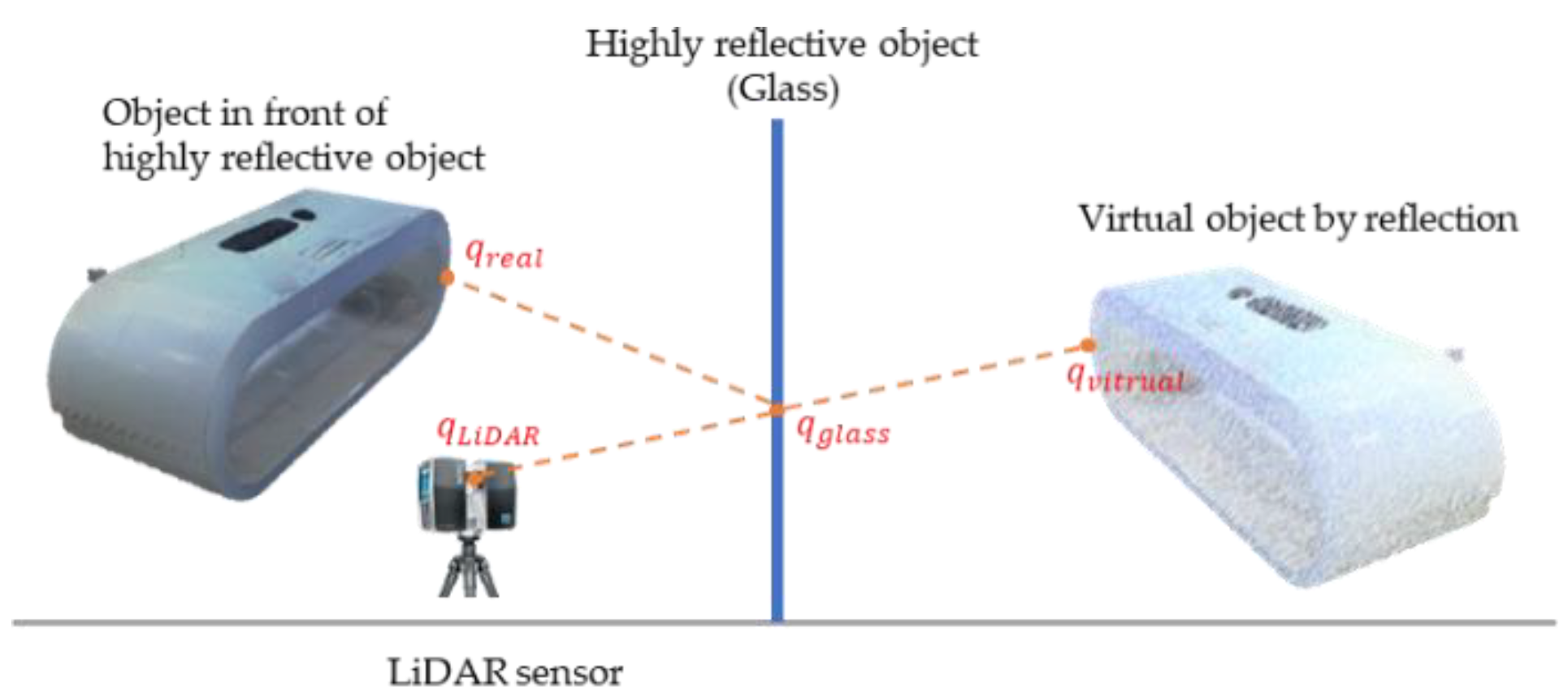
LiDAR sensors measure the distance between the scanner and target object by transmitting laser pulses and receiving the return pulses. Reflective materials (such as glass, displays, and walls with smooth surfaces) cause the return pulses received by the LiDAR to be perceived as linear reflected pulses reaching the scanned object. In other words, when using a LiDAR scanner to capture a 3D real scene, a single laser pulse from the scanner initially hits the surface of reflective materials, and its echo pulse returns to the scanner to create a 3D point on the glass plane. In addition, the penetration and reflection of light occur simultaneously on reflective materials. The penetrating laser pulse hits the real object front of the reflective materials, and its echo pulse is received by the scanner to generate another 3D point [4], as shown in Figure 1. When the laser emitted by LiDAR hits the glass at a certain angle, the nature of the glass reflects the laser to other locations ( in Figure 1), however, LiDAR is not aware of the presence of the glass, so it registers the position of at . In this study, only specular reflections at specific angles are considered. The effect caused by the refraction of the glass is not presently included. All objects capable of producing specular reflections are referred to as reflective materials and we refer to the noise due to reflective materials as reflective noise; this noise accounts for most of the noise in the data used in this study. Therefore, this study aimed to automate the elimination of noise due to specular reflections from reflective materials. Prior to this study, the scan data used in point-cloud detection and denoising research [3] were essentially scan datasets of small scenes or single objects. Specifically, a dataset, different to those used in previous studies, was employed in this study. This dataset consists of a large scene containing a variety of reflective materials, and the number of points and noise point densities are extremely high.
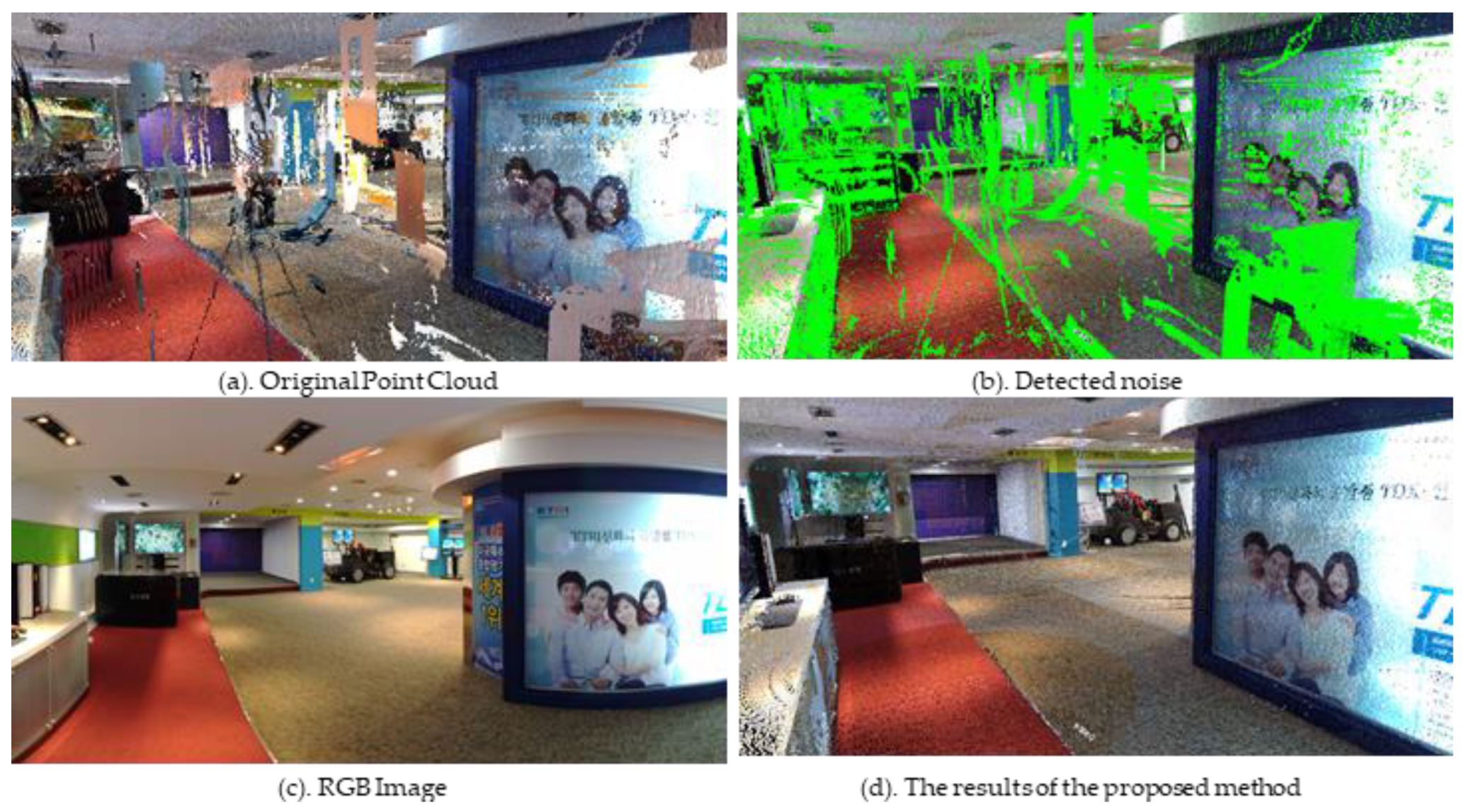
Contemporary methods for removing 3D point-cloud noise are usually performed on the point-cloud data of a single object, where the number of points is not particularly large, or the point density is sparse. The number of point cloud points of a single scene used in this study is approximately 40 million, of which, there are approximately 10,000 reflection noise points. The total number of point clouds used in other denoising algorithms [3] is approximately 30,000. Therefore, the noise scale of the point cloud used in this study is huge and dense. Although traditional point-cloud noise filtering methods can effectively remove outliers from dense point clouds, they cannot effectively detect and remove dense noise or noise regions generated by reflective materials. This is because the point density of the noise area generated by the reflection is extremely dense, and thus, the local noise detection and removal method cannot be effectively performed. The dataset used in this study contains scan data from large indoor scenes with rich scene information. The noise generated by reflective materials is the sampling of real objects in front of the glass, outlined in Figure 2.
Recently, deep learning technology has dominated many research fields, such as computer vision, speech recognition, and natural language processing. Deep learning offers a new paradigm in 3D point-cloud detection and denoising technologies. With the advancement of deep learning, researchers have been inspired to combine two-dimensional (2D) image analysis and deep learning in the application of 3D point clouds. This study proposes the use of a reflection value range image extracted from 3D LiDAR data as the input, which is then combined with a transformer auto-encoder network to detect the noise generated by an object with high reflection intensity in the point-cloud data. Unlike the 3D convolution, which needs to convert the input into a regular grid, our proposed method directly extracts the reflection value range image from the 3D LiDAR data into 2D image data and uses it as input. The noise region is marked out using the transformer network [5], and then, precise marking is performed using the multi-position comparison method, and finally, the denoised point cloud is obtained.
Compared to our preliminary study [6], the contributions of this paper are as follows:
- To the best of our knowledge, this study is the first to use deep learning for denoising large-scale point clouds containing only single-echo reflection values.
- In our preliminary study [6], the denoising effect is adjusted by manually setting parameters, which requires some knowledge of the dataset. This study uses deep learning to automate noise detection without the need for manual parameter tuning.
- Through qualitative and quantitative evaluations, the methods proposed in this study were superior to the previous methods [6].
2. Related Works
In this section, we review several established methods employed for 3D point-cloud denoising, mainly in two categories: traditional methods and deep learning methods. Few studies have been conducted for large-scale, high-density point-cloud denoising, and we present them separately in Section 2.3.
2.1. Traditional Method
There are several traditional methods for denoising 3D point clouds. However, most of these methods are based on filtering methods, which denoise the 3D point cloud of a single object. For example, kernel-based clustering methods move points to high-probability locations and employ statistical-based filtering techniques to smooth point clouds through an iterative scheme of mean shift technique channels [7]. These technique channels employ a mean drift-based clustering process and filtering method to suppress noise of different amplitudes and allow a simple outlier detection followed by a simple threshold for automatic removal. The remaining great likelihood points then provide an accurate point-based approximation of the surface. Kalogerakis et al. [8] provided a robust statistical framework to filter point clouds. The framework estimates the curvature tensor in an iterative least squares (IRLS) approach and assigns weights to the samples at each iteration to refine each domain around each store. The robustly estimated curvature and normal provide a global energy minimization process to drive outlier point-cloud suppression and denoising in a feature-preserving manner. Jenke et al. [9] proposed a surface reconstruction method based on Bayesian statistics. The method models the measurement process and prior assumptions about the measured object as a probability distribution and uses Bayesian rules to infer the reconstruction with maximum probability. The method is robust for general reconstruction of a priori unknown topological models and removes noise while preserving and explicitly reconstructing sharp features. Domain-based filtering methods use a similarity measure between a point and its neighborhood to determine the filtering location of that point, which can be defined by the location of the point, the location of the normal, or the location of the region. Tomasi and Manduchi et al. [10] introduced the concept of bilateral filters for edge-preserving smoothing, which was further extended to 3D mesh denoising by Fleishman et al. and Jones et al. [11,12]. However, be-cause the noise is inherent in the 3D grid, bilateral filtering based on point position and intensity was applied directly to the point cloud [13]. Schall et al. [14] extended the image filtering non-local mean method to 3D point clouds based on a similar idea of bilateral filtering. They introduced a new non-local similarity metric that considers the local square neighborhood around the store. This method yields more accurate filtering results and superior feature retention properties.
The projection-based filtering method filters point clouds by adjusting the position of each point in the point cloud through different projection strategies. Lipman et al. [15] introduced the local optimal projection (LOP) operator to denoise 3D point clouds. However, the method becomes non-uniform in the projection when the input point-cloud height is not uniform, which is undesirable in terms of both shape feature preservation and normal score estimation. Liao et al. [16] proposed a method called spatial–temporal LOP operator (STLOP), which is used for the geometric reconstruction of feature-preserving LOP operators (FLOPs). The method uses an accelerated FLOP operator based on kernel density estimation (KDE) random sampling. This sampling method produces reconstruction results similar to those produced using the complete point set data and within a given accuracy range. Preiner et al. [17] designed an efficient variant of a locally optimal projection operator. The method uses a Gaussian mixture model formed by the regularized hierarchical EM algorithm to cluster points that represent the density of the point cloud. Wang et al. [18] proposed an algorithm that includes two steps: outlier filtering and noise smoothing. The method designs a connectivity-based approach to remove sparse outliers based on the relative deviations of local neighborhoods and the properties of local neighborhoods of flat clouds and achieved satisfactory results. Signal processing methods can also be extended to point-cloud filtering. Pauly et al. [19] introduced a discrete approximation of the Laplace operator to point clouds. They proposed a framework and algorithm for the edge-resolution modeling of point sampling geometry that can effectively produce significant model deformations. However, this approach can smoothen properties, consequently resulting in vertex drift. Pauly and Gross [20] used the spectral processing of point clouds for filtering. This method computes a set of add-window Fourier transforms to create a spectral decomposition of the model. The direct analysis and manipulation of spectral sparsity supports effective filtering, resampling, power spectrum analysis, and local error control. This method allows the direct manipulation of points and normal without the need for vertex connectivity information.
The aforementioned point-cloud filtering method can be effective in removing outliers from point clouds in specific cases, such as point-cloud models with added Gaussian noise. However, it is not effective in removing reflection noise in the form of non-anomalies.
2.2. Deep Learning Method
In recent years, deep learning methods have achieved great success in the denoising of 2D images and object detection, but it is more difficult to process point clouds than 3D images because of the irregular structure of 3D point clouds [21]. With the advent of PointNet [22], point-cloud processing based on deep learning has become easy, and several methods for 3D point-cloud denoising have been proposed in the literature [23,24,25,26,27]; however, these methods use data obtained by adding random noise to the point cloud and do not work for point clouds actually acquired using LiDAR. Deep learning research for direct denoising of point clouds is scarce, so this study also refers to various deep learning-based work on point-cloud processing.
Wu et al. [28] proposed a new convolutional operation named PointConv. This operation is applied to build deep convolutional networks on point clouds, which can fully approximate the 3D continuous convolution on any set of 3D points and directly perform semantic segmentation on 3D point-cloud data. The network built on PointConv can match the convolution on 2D images of similar structure network performance. Lei et al. [29] proposed an octree-guided neural network architecture and spherical convolution kernel for machine learning from 3D point clouds. The proposed spherical kernel system quantizes point neighborhoods to identify local geometric structures in the data, while simultaneously keeping the reviews undeformed and asymmetric. Lan et al. [30] proposed the GeoCNN network, which applies a generic convolution operation, referred to as GeoConv, to each point and its local domain. GeoConv explicitly models the geometric structure between two points by decomposing the feature extraction process into three orthogonal directions and aggregating features based on the angle between the edge vector and the basis. Mao et al. [31] proposed an InterpConv layer-based interpolated convolutional neural network (InterpCNNs) to solve the problem of point-cloud feature learning and understanding. This operation uses a set of discrete core weights to interpolate point features to adjacent core weight coordinates through an interpolation function for convolution to process point-cloud recognition tasks, including shape classification, partial object segmentation, and indoor scene semantic analysis. Zhang et al. [32] proposed a RIConv operator to achieve point-cloud rotation without deformation. This operator considers low-order rotation invariance geometric features as input and solves point sorting by seamlessly constructing a boxing method in the convolution problem. Subsequently, the convolution operator is used as the basic component of a neural network, which is robust to the point cloud under the 6-DoF transformation. Liu et al. [33] proposed a new 3D point-cloud deep learning model—Point2Sequence. The model obtains relevant information by concentrating the multi-scale areas of each local area. Jiang et al. [34] designed a module called PointSIFT, which realizes multi-scale representation by superimposing multiple directional coding units. This module can be integrated into various point-net-based architectures to improve presentation capabilities.
2.3. Reflection Noise Removal for Large-Scale 3D Point Clouds
The methods mentioned above are all used for small-scale point clouds, where most of the data are processed and validated by adding random noise similar to a clean point cloud, which can simulate, to some extent, the random errors generated when collecting point clouds in devices like LiDAR. However, it is not possible to target the high density of noise due to reflective materials. Yun et al. [35] proposed a method to detect reflected noise based on the number of echo pulses of the emitted laser pulse. They then further proposed a reflection noise removal method for removing multiple glass planes in a large-scale point cloud [4]. Gao et al. [6] proposed a method to extract the features of reflection noise by using sliding windows and calculating the variance, which achieved good results, but required manual adjustment of the parameters. To the best of our knowledge, there are no studies, other than the ones mentioned above [4,6,35], that can automate the removal of reflection noise from large-scale point clouds. Additionally, this literature [4,35] uses point-cloud data with multiple echoes, which does not apply to point-cloud data containing only single-echo reflection intensity data.
3. Proposed Method
In a previous study [6], the characteristics of the reflective noise region were summarized. Since the reflections were generated by LiDAR irradiation to the reflective material, the obtained reflection values were confusing compared to other normal objects. Therefore, in this study, the reflection value information of all points from the point-cloud image scanned from a single scene are extracted and converted into a 2D range image, and then, a transformer network is used to detect the reflection noise region for the range images. The edges where two objects meet also produce reflectance value transformations similar to noise regions, which cannot be recognized by the transformer network. Hence, the results obtained from the transformer network are used in this study for more detailed noise detection and removal, and the multi-position comparison method is used to further improve the accuracy.
3.1. System Overview
The dataset used in this study is a large-scale scene comprising multiple scan data, which not only contains a variety of objects, but also contains a large number of reflective materials with high reflection intensity. The purpose of this research is to detect and remove high-density reflective noise caused by reflective materials with high reflection in-tensity. By analyzing the noise-generating area in the point-cloud data, reflective mate-rials that generate a wide range of noise areas are defined to have high reflectance [6]. Therefore, to accurately detect the reflection noise area with high reflection intensity in the point-cloud data, this study uses the transformer auto-encoder method, which has a significant effect on the detection of noise areas in 2D images caused by objects with high reflectance characteristics.
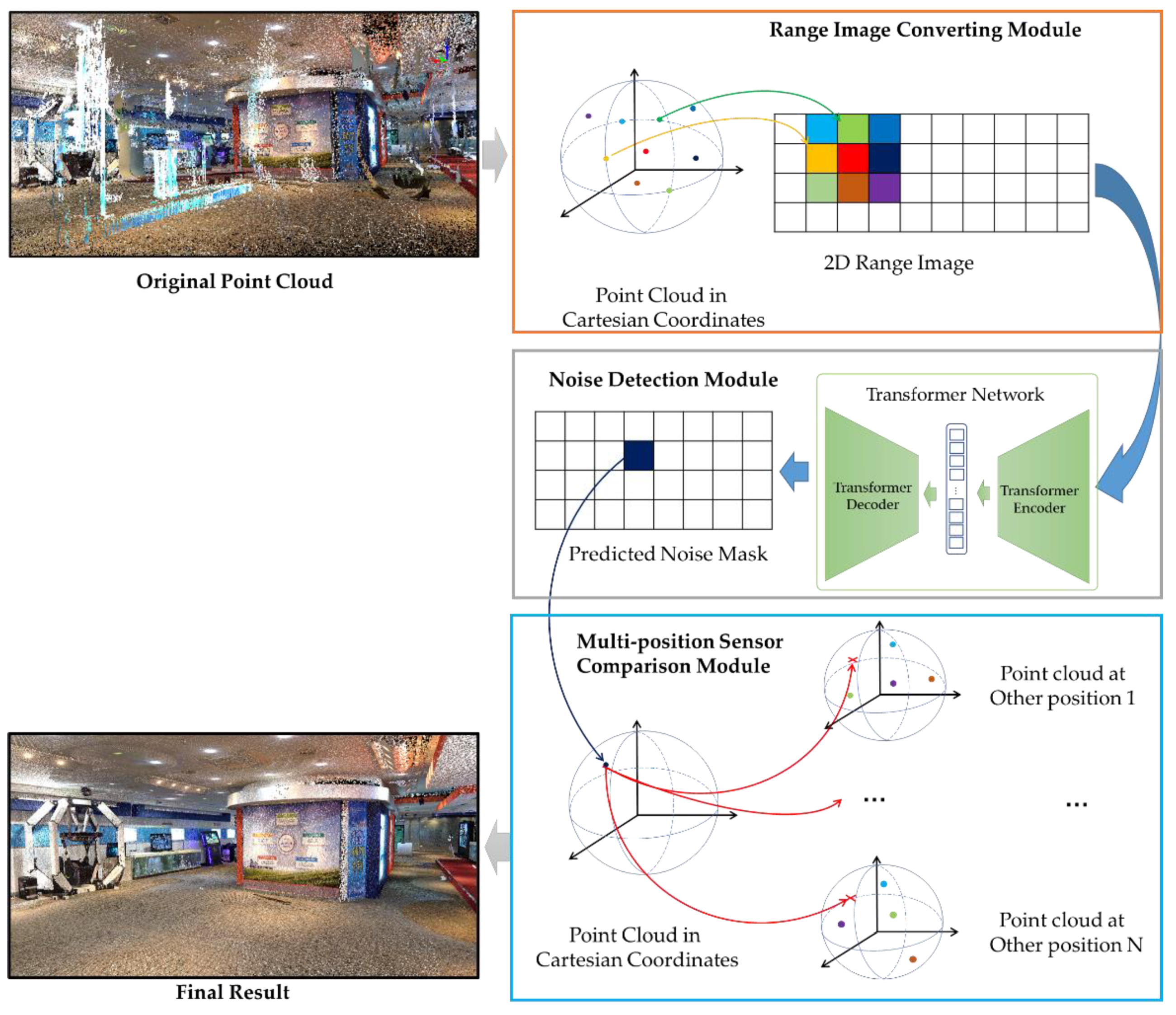
The data used in this study are 3D point-cloud data collected by LiDAR from several different locations in the same scene using LiDAR devices. This study will perform noise detection for the point-cloud data collected at a single location, then finally remove the noisy area by comparing it with the point-cloud data from other locations. The first part of the method involves the range image converting module, which converts the 3D point-cloud data into a 2D range image; the second part is the noise detection module, which uses the transformer for noise detection; the third part is the multi-position sensor comparison module, which compares the results of the second part with the sensor data from other positions and generates the denoised point-cloud data. These three parts are outlined in Figure 3.
3.2. Range Image Converting Module
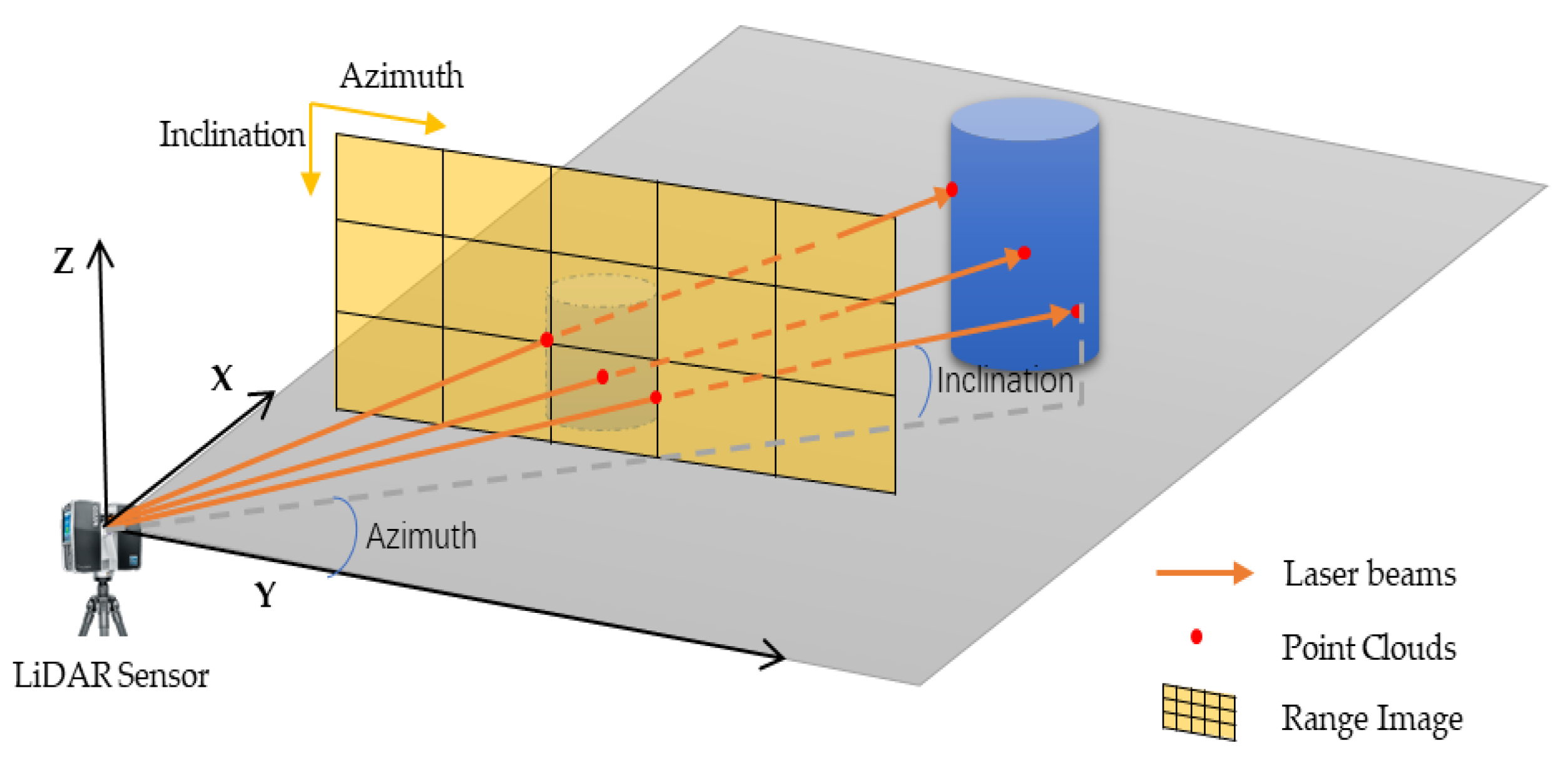
In the first stage, the LiDAR position XYZ, color RGB, and reflection value denoting seven channels of information are included in the laser radar scan data. The 3D LiDAR sensor obtains multiple beams and multiple measurements from one scanning period, and the returned value forms a distance picture. The pixel value in the distance picture contains the distance of the corresponding point and the intensity of the returned laser pulse, along with other auxiliary information. A 2D image is formed by extracting the intensity of the returned laser pulse. Each scan line contains the same number of dots, and the scan lines are stacked horizontally to form similar structures. Therefore, any measurement value of the sensor is arranged in a 2D image [36]. Hence, we can convert a piece of 3D point-cloud data into a 2D picture. The pseudocode for converting 3D point-cloud data into a 2D image is defined in Algorithm 1.
| Algorithm 1. Converting 3D point-cloud data into a 2D image. |
|
In the laser radar scan data, there are seven pieces of information regarding the LiDAR positions X, Y, Z, colors R, G, B, and reflection value. Therefore, based on the description in [6] and according to the 3D point-cloud data, the reflection value contained in each point of the LiDAR scan data can be extracted from the 3D point-cloud reflection intensity value data and mapped to a 2D image sequentially. It is then converted into a 2D reflection range image, as shown in Figure 4.
Because the scan data of each 3D point cloud in the dataset used in this study are significantly large, the size of the 2D range image is also large, at 10,330 × 4268. Hence, directly inputting the converted 2D reflection range image into the transformer network will not allow the deep learning network to effectively detect the noise area in the 2D reflection range image. Therefore, before inputting the 2D reflection range image into the transformer network, each image is cropped to a size of 512 × 512.
3.3. Range Image-Based Noise Detection Module
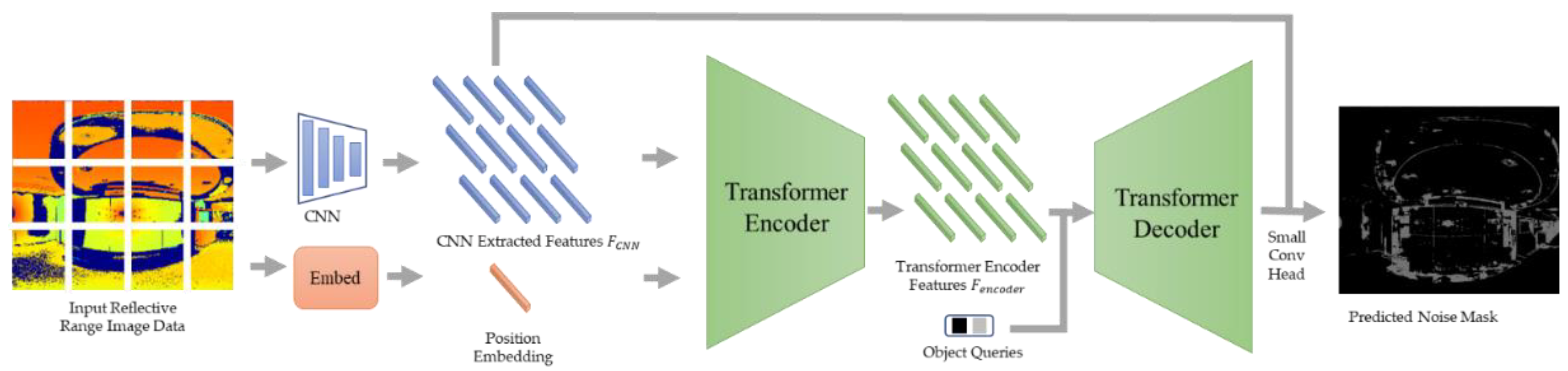
This module treats noise detection in the range image as a semantic segmentation problem of the image and uses a transformer auto-encoder network [5] with manually denoised point clouds as the ground truth for training. The input image is a segmented reflective range image, and, after semantic segmentation using the transformer auto-encoder network, the output mask map contains only two classifications: noise and normal regions.
First, the input reflective range image is fed to the CNN to extract the features . Second, for the transformer encoder, the features and location embeddings are spread and fed to the transformer for self-attention, and the features are output from the transformer encoder. Third, for the transformer decoder, we specifically define a set of learnable class prototype embeddings as queries and as keys and compute the attention map using and . Each class prototype embedding corresponds to a final predicted class. The small conv head is used here to fuse the attention map and Res2 features from the CNN backbone, as shown in Figure 5.
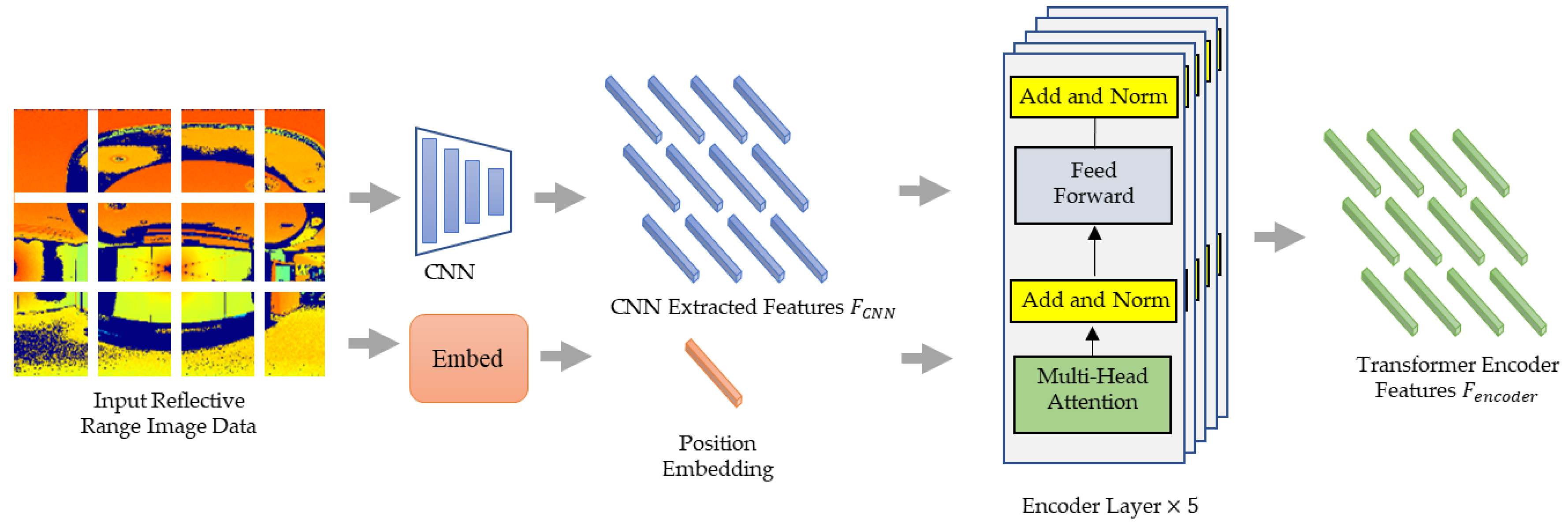
Since transformer encoders consider a sequence as input, the range image extracted from the 3D radar data is input to the image feature map extracted from the CNN backbone, flattened into one dimension, and the flattened image is then input into a one-dimensional (1D) image feature map in the encoder to compensate for the missing spatial information. The position code is added to the 1D feature, which is then used to provide the relative or absolute position information of the feature. The features extracted by the encoder are used as the input of the decoder. The transformer encoder is composed of multiple encoder layers, with each layer consisting of a multi-head self-attention module and a feed-forward network, as shown in Figure 6.
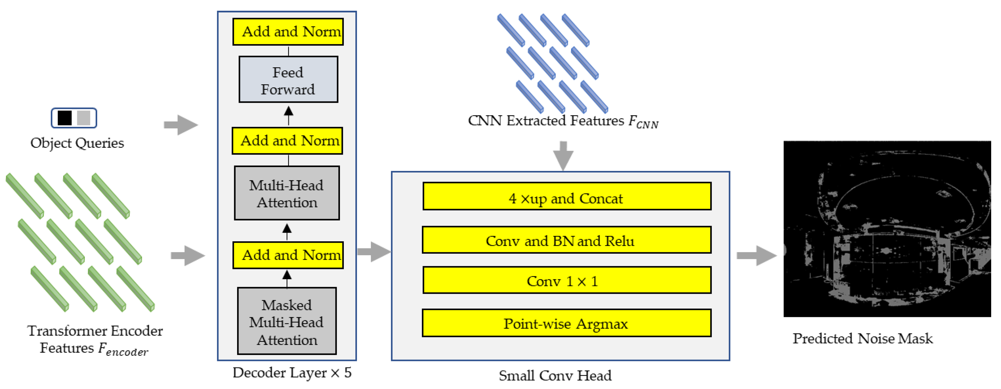
The transformer decoder considers features from the transformer encoder as keys and values, then combines them with object query prototypes to obtain a query as input for the transformer decoder. The decoder consists of five stacked identical decoder layers. In addition to the masked multi-head attention module and feed-forward network sub-layers, each decoder layer also inserts a third sub-layer, which performs multi-head attention on the output of the encoder layer and embeds a set of learnable class prototype embedding (the prototype embedding of each class corresponds to a final predicted category) as queries. The transformer decoder takes as input a set of learnable class prototype embeddings as queries, denoted by . The encoded features as keys and values are recorded as , and the final noise mask result is obtained by outputting the attention map followed by Small Conv Head. Class prototype embeddings are learned category prototypes that are iteratively updated by a series of decoder layers through a multi-headed attention mechanism. We use ⨀ to denote the iterative update rule, then the class prototype for each decoding layer is:
In the final decoder layer, the attention graph is extracted into the small conv head:
The attention map from the decoder represents the shape of C, M, H/16, and W/16, where C is the class number and M is the number of heads in multi-head attention. The attention map is upsampled and the final output attention map shape is C, H/4, and W/4. Subsequently, a pixel-wise argmax operation is performed on the output attention map and, finally, the detection result is obtained, as shown in Figure 7.
The input to this part is a learnable category prototype as the object query and features from the transformer encoder as keys and values. The input is fed to a transformer decoder consisting of five decoder layers. The attention map from the last decoder layer and the Res2 features from the CNN backbone are combined and fed to a small conv head to obtain the final prediction results.
After all datasets were detected using our proposed method, we combined the detected noise results using the multi-position sensor comparison method to further improve the detection accuracy and delete the noise in the final detection results. After removing all of the noise regions, we reconstructed the 3D point cloud from the noise-removed 2D range image and restored the 2D range image to the 3D point-cloud data form.
3.4. Multi-Position Sensor Comparison Module
If the results of the transformer are solely used for noise region removal after obtaining the results of the noise detection module, some normal points will be removed at the same time, since the edges of the noise region will contain some normal points. Therefore, in order to improve the accuracy of noise region removal, we used the multi-position sensor comparison module provided by the previous method [6] for fine noise detection.
The multi-position sensor comparison compares the LiDAR information of the selected target that requires noise detection with the LiDAR information of the relatively close surrounding areas. The different point-cloud information in the compared LiDAR scan data is then deleted to obtain the detection result. Specifically, the multi-position sensor comparison module first reads the position information of all sensors, then selects several suitable sensor data to load into the k-d tree according to the position information of the currently processed sensors. Subsequently, according to the result of the transformer for the noise region with the other position. The point-cloud data collected by the sensors are then compared. Since the location of noise is not fixed in the point clouds collected by different sensors at different locations, if the points do not exist in the other sensors, they are considered noise points. Hence, by using the multi-position sensor comparison module, an accurate denoised point-cloud data can be obtained in this study.
4. Experiments
The primary purpose of this study is to detect and remove the noise generated by objects with high reflection intensity in 3D point-cloud LiDAR data. In the detection of 3D point-cloud LiDAR data from large scenes, the proposed method converts the 3D point-cloud data into a 2D range image without losing the 3D point-cloud LiDAR data and discards the original input RGB image. To perform the reflective materials detection method, the reflection value range image is input to complete the preliminary detection of the noisy area, based on the high reflection value characteristic of the reflective materials that produce noise. Subsequently, the 2D range image, after noise removal, is reconstructed into a 3D point cloud to complete the noise removal of the 3D point-cloud radar data.
4.1. Implementation Details
The transformer auto-encoder network [5] used in this study implemented the noise detection module. We implemented the transformer auto-encoder network with Pytorch. For loss optimization, we used the Adam optimizer with epsilon set to 1 × 10⁻⁸ and weight decay set to 1 × 10⁻⁴. The batch size was 4 per GPU. We set the learning rate as 1e-4 and decayed the poly strategy [37] for 50 epochs. We used 2 Titan GPUs for training. For all CNN based methods, we random scaled and cropped the images to 512 × 512 in training, and resized the images to 512 × 512 in inference, following the common settings of PASCAL VOC [38].
4.2. Experiment Environment and Dataset
Our proposed method was implemented in a Linux operating system and two Nvidia TITAN V GPUs. Two Intel(R) Xeon(R) Silver 4114 CPUs running Python 3.7 were configured for the system. The data used in this study was a real indoor scene captured by FARO Focus 3D X 130 [39]. The main data were obtained from the ETRI exhibition hall, with an area of about , and contained a large number of exhibition areas and reflective materials (e.g., glass, displays, smooth walls, etc.). Point-cloud data were collected from a total of 72 different locations in the ETRI pavilion. The majority of the scanners used default settings. Some of the settings data are provided in Table 1, however, this can be changed for different scenarios. Here, we only provide the more typical scanner settings data. The point-cloud registration is courtesy of FARO SCENE [40].
Table 2 shows the number of point clouds for four of the scenes, each with roughly 40 million points due to the noise in all data. The number of noise points generated varies widely due to the location and amount of reflective materials in different locations in the scene. In our previous work [6], abbreviated as MPMC (manual parameter multi-position comparison) in this study, we manually denoised the point-cloud data from 19 of these locations.
Table 3 shows the comparison between the dataset used in this study and other datasets. The datasets used in this study all greatly exceed the other datasets in terms of the number of points. The amount of noise in the dataset used in this study is larger than the total number of point clouds in one scan of a single object. In the PointCleanNet Dataset [24], noisy point clouds are generated by adding Gaussian noise with the standard deviations of 0.25%, 0.5%, 1%, 1.5%, and 2.5% of the original shape’s bounding box diagonal [24]. Additionally, in LS3DPS [35,36], their objectives are consistent with this paper, but the total amount of noisy data is not indicated in their data.
In this study, we used these 19 manually denoised point-cloud data points as the ground truth for training and validation. The specific data division is shown in Table 4.
4.3. Noise Detection and Performance
This study used the same evaluation criteria as [41] to analyze the proposed method. The four values of the outlier detection rate (ODR), inlier detection rate (IDR), false positive rate (FPR), and false negative rate (FNR) were used as the evaluation criteria. In this section, outliers are defined as noise to facilitate the calculation of the formula. In the ODR formula, a higher outlier detection rate increases the amount of noise that our method is able to detect. In the IDR formula, a higher inlier detection rate increases the number of normal points that our method can detect. A high FPR indicates more noise points being detected as normal points in the proposed method. A high FNR indicates a higher value of normal points being detected as noise. In summary, higher ODR and IDR values and lower FPR and FNR values indicate an enhanced performance of detection abilities of our proposed method. Combining the aforementioned four ratios, the accuracy rate illustrates the overall effectiveness of the proposed method in detecting abnormal values. In the below formulas,
TP and TN indicate the number of outliers and inliers that are correctly defined, respectively.
Table 6 shows the accuracy of the results of the proposed method and presents the comparison results of FARO [40], MPMC [6], and our method. The accuracy is calculated using Equation 7, where the accuracy represents the proportion of correctly detected points (including outliers and inliers) among all point clouds. Since the density of the point clouds and the percentage of normal points are very high, the values of accuracy are all relatively high. However, the accuracy of the method proposed in this study is the highest among the methods tested.
The performance of the various methods is compared in Table 7 by comparing their ODR, IDR, FPR, and FNR values, and higher values of ODF and IDR and lower values of FPR and FNR indicate better performance.
Table 8 compares the computational resources used for each of the methods examined in this experiment.
Figure 8 shows the denoising effect of the method proposed in this study on a single sensor data point. Since the noise regions in the individual point-cloud data are discrete, we will use the image after merging all point-cloud data in the subsequent presentation of the results.
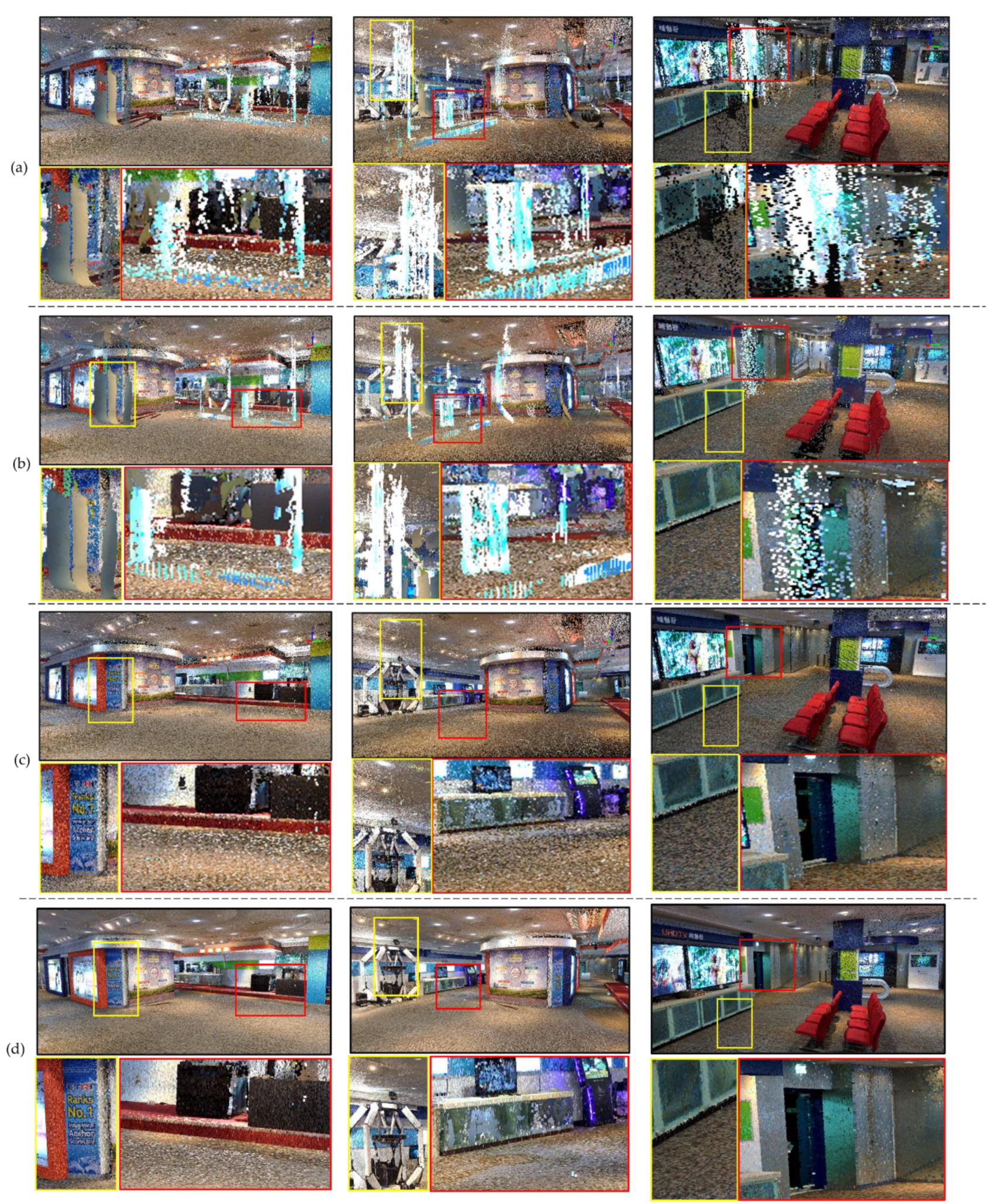
Figure 9 outlines the results obtained by the proposed method, the FARO SCENE method [39], and the MPMC method [6]. The figure shows noise locations in three different regions and the results of denoising using the different methods.
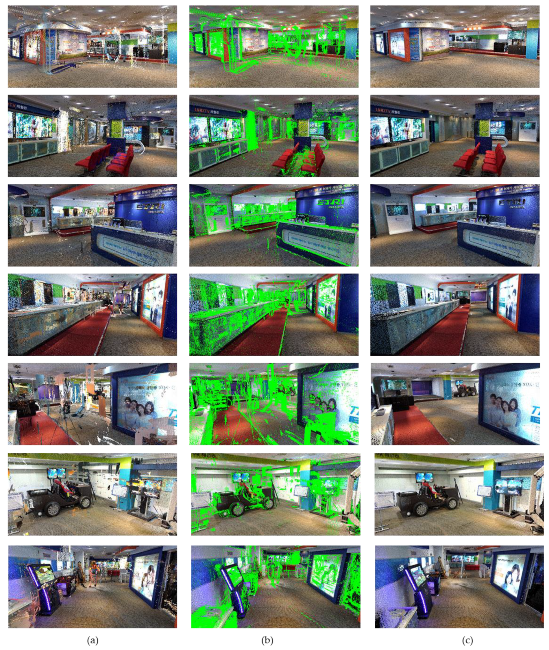
Figure 10 shows the data from the ETRI showroom. There is a total of 72 point clouds collected by sensors at different locations in this scene, and the results outlined in this figure are the result of combining all of the point-cloud data together.
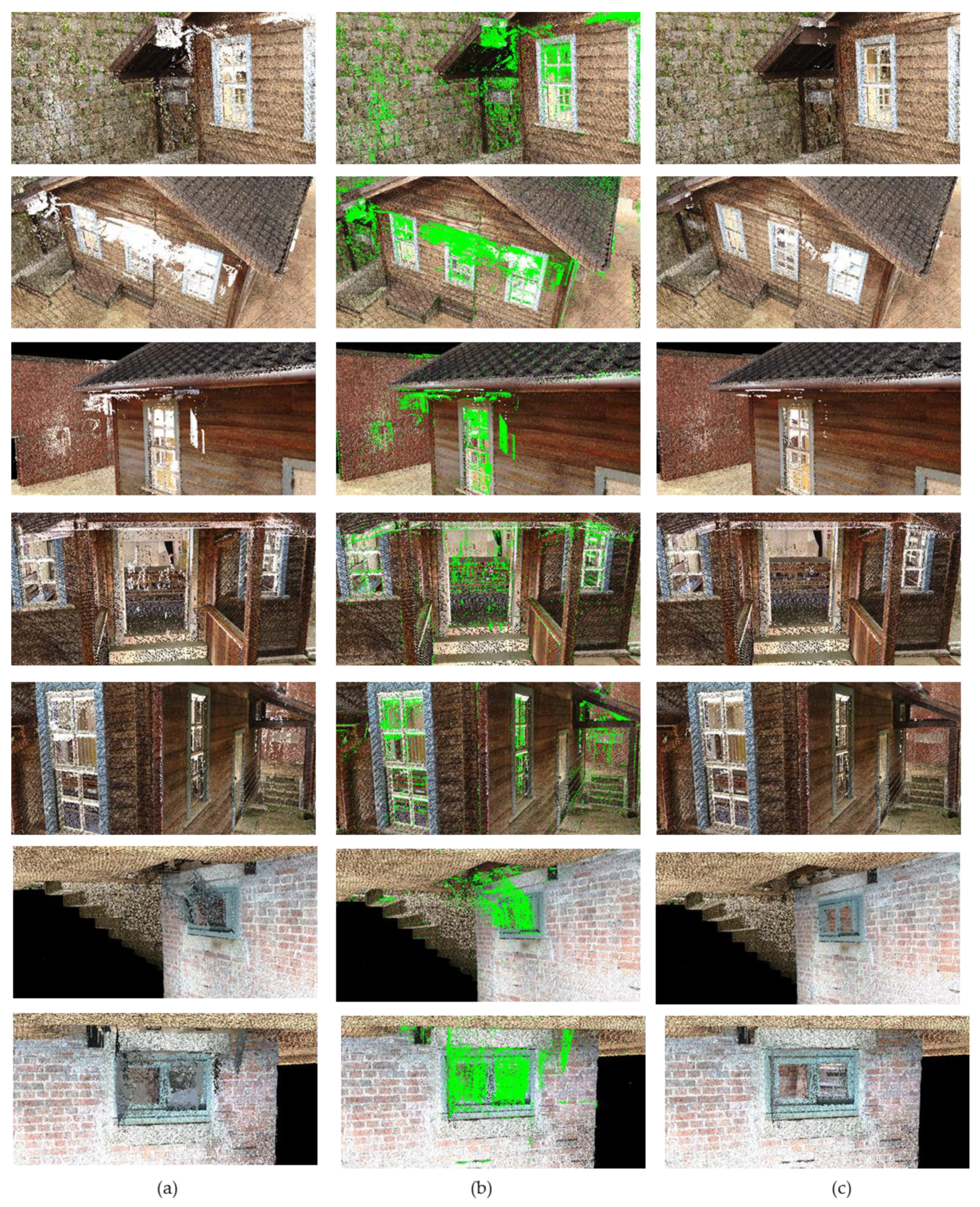
Figure 11 shows results for other datasets from a total of 190 different locations where the point-cloud data were collected. The figure shows the results after merging all data.
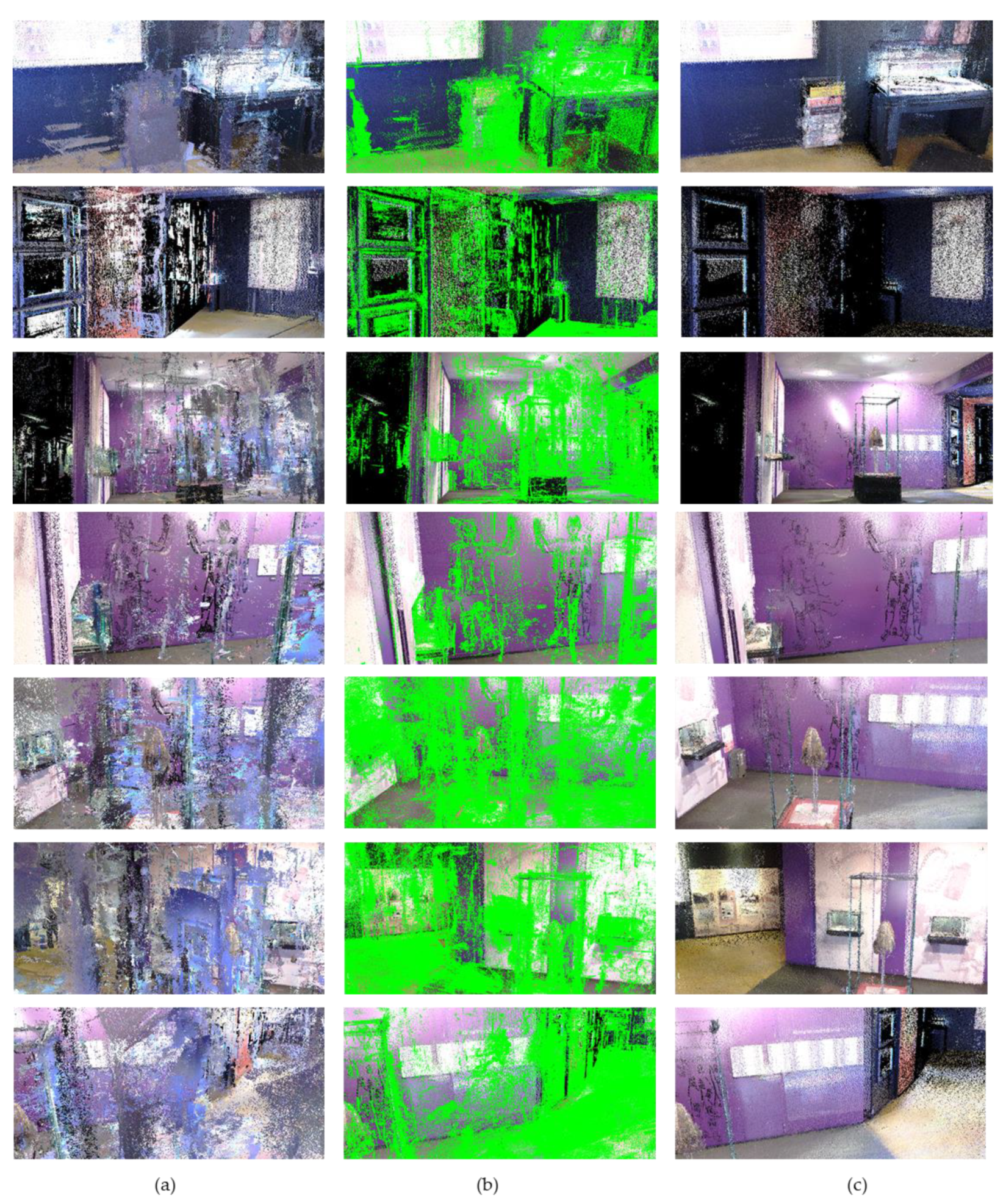
Figure 12 outlines results for additional datasets from a total of 39 different locations where the point-cloud data were collected. The figure shows the results after merging all data.
5. Conclusions
This study proposed a new method for detecting noise with high reflection intensity in 3D point-cloud LiDAR data. The proposed method first converts the 3D point-cloud LiDAR data into a 2D range image, then extracts the reflection value range image as the input for the transformer auto-encoder network. The feature map is output by the encoder and used as the input for the decoder to detect objects with high reflection intensity that generate noise. Experiments show that the proposed method, compared with traditional methods, can effectively detect the noise area generated by reflective materials, or objects with high reflectance, in large-scale scanning scenes containing rich object information. To determine the validity of the proposed method, 3D point-cloud LiDAR data from several different scenes were tested. The transformer auto-encoder was used to process the 2D image data of the large-scale point cloud, and the noise area, generated by reflective materials or objects with high reflection values, in the 2D image data was detected. Specifically, noise point-cloud detection of large-scale 3D point-cloud scenes provides a new perspective on the subject matter.
Since LiDAR is reflected by reflective materials and causes a large amount of noise in the captured point cloud, some studies have analyzed the effect of reflective materials on LiDAR and proposed some solutions. However, these studies have used sparse point-cloud data or focused on detecting the location of reflective materials rather than removing the noise generated by them. In our previous study, we analyzed and summarized the noise region generated by reflective materials. The noise region is chaotic compared to other objects due to the reflection of the laser, hence, the current study used the transformer network to detect the noise region. Experiments show that the method proposed in this study can effectively remove high-density reflective noise caused by reflective materials. Unlike other studies that target individual object surfaces for noise removal methods, this study uses the characteristics of the reflection intensity of LiDAR for noise determination and achieves good results in different scenes. This study showed that the method has wide applicability and can effectively eliminate the influence of reflective materials on point clouds. To the best of our knowledge, this paper is the first study to use a deep learning method to perform reflection noise cancellation on a large-scale point cloud containing only single-echo reflection values. Moreover, compared with previous work, this paper substantially improved the processing speed and improved performance.
It is essential to continue to explore the task of noise detection noise in the transformer auto-encoder network to improve the accuracy of detection; this will be considered in future studies. Additionally, in future studies, the dataset should not be limited to large indoor scenes, but also include large outdoor scenes (such as cities or streets). In addition to detecting the noise area generated by reflective materials or objects with high reflection intensity, the types of objects detected should be expanded, thereby enhancing the versatility of the proposed method, providing further scope for future research.
Author Contributions
Conceptualization, R.G.; data curation, M.L.; funding acquisition, K.C.; methodology, R.G. and M.L.; project administration, K.C.; supervision, K.C.; writing—original draft, R.G. and M.L.; writing—review and editing, S.-J.Y. and K.C. All authors have read and agreed to the published version of the manuscript.
Funding
This work was supported by Electronics and Telecommunications Research Institute (ETRI) grant funded by the Korean government. [21ZH1200, The research of the fundamental media·contents technologies for hyper-realistic media space].
Institutional Review Board Statement
Not applicable.
Informed Consent Statement
Not applicable.
Data Availability Statement
The data presented in this study are available on request from the corresponding author. The data are not publicly available due to that the information of cultural relics and the research facilities is involved, that cannot be opened without authorization.
Conflicts of Interest
The authors declare no conflict of interest.
References
- Guo, Y.; Sohel, F.; Bennamoun, M.; Lu, M.; Wan, J. Rotational Projection Statistics for 3D Local Surface Description and Object Recognition. Int. J. Comput. Vis. 2013, 105, 63–86. [Google Scholar] [CrossRef] [Green Version]
- Guo, Y.; Bennamoun, M.; Sohel, F.; Lu, M.; Wan, J. 3D Object Recognition in Cluttered Scenes with Local Surface Features: A Survey. IEEE Trans. Pattern Anal. Mach. Intell. 2014, 36, 2270–2287. [Google Scholar] [CrossRef] [PubMed]
- Han, X.-F.; Jin, J.S.; Wang, M.-J.; Jiang, W.; Gao, L.; Xiao, L. A review of algorithms for filtering the 3D point cloud. Signal Process. Image Commun. 2017, 57, 103–112. [Google Scholar] [CrossRef]
- Yun, J.-S.; Sim, J.-Y. Virtual Point Removal for Large-Scale 3D Point Clouds with Multiple Glass Planes. IEEE Trans. Pattern Anal. Mach. Intell. 2019, 43, 729–744. [Google Scholar] [CrossRef] [PubMed]
- Xie, E.; Wang, W.; Wang, W.; Sun, P.; Xu, H.; Liang, D.; Luo, P. Segmenting Transparent Object in the Wild with Transformer. arXiv 2021, arXiv:2101.08461. [Google Scholar]
- Gao, R.; Park, J.; Hu, X.; Yang, S.; Cho, K. Reflective Noise Filtering of Large-Scale Point Cloud Using Multi-Position LiDAR Sensing Data. Remote Sens. 2021, 13, 3058. [Google Scholar] [CrossRef]
- Schall, O.; Belyaev, A.; Seidel, H.-P. Robust filtering of noisy scattered point data. In Proceedings of the Eurographics/IEEE VGTC Symposium Point-Based Graphics, Stony Brook, NY, USA, 21–22 June 2005; pp. 71–144. [Google Scholar]
- Kalogerakis, E.; Nowrouzezahrai, D.; Simari, P.; Singh, K. Extracting lines of curvature from noisy point clouds. Comput. Des. 2009, 41, 282–292. [Google Scholar] [CrossRef]
- Jenke, P.; Wand, M.; Bokeloh, M.; Schilling, A.; Straßer, W. Bayesian Point Cloud Reconstruction. Comput. Graph. Forum 2006, 25, 379–388. [Google Scholar] [CrossRef]
- Schall, O.; Belyaev, A.; Seidel, H.-P. Adaptive feature-preserving non-local denoising of static and time-varying range data. Comput. Des. 2008, 40, 701–707. [Google Scholar] [CrossRef]
- Fleishman, S.; Drori, I.; Cohen-Or, D. Bilateral mesh denoising. In ACM SIGGRAPH 2003 Papers; ACM: San Diego, CA, USA, 2003; pp. 950–953. [Google Scholar]
- Jones, T.R.; Durand, F.; Desbrun, M. Non-iterative, feature-preserving mesh smoothing. In ACM SIGGRAPH 2003 Papers; ACM: San Diego, CA, USA, 2003; pp. 943–949. [Google Scholar]
- Ma, S.; Zhou, C.; Zhang, L.; Hong, W.; Tian, Y. Depth image denoising and key points extraction for manipulation plane detection. In Proceedings of the 11th World Congress on Intelligent Control and Automation, Shenyang, China, 29 June–4 July 2014; pp. 3315–3320. [Google Scholar]
- Schall, O.; Belyaev, A.; Seidel, H.P. Feature-preserving non-local denoising of static and time-varying range data. In Proceedings of the 2007 ACM Symposium on Solid and Physical Modeling, Beijing, China, 4–6 June 2007; pp. 217–222. [Google Scholar]
- Lipman, Y.; Cohen-Or, D.; Levin, D.; Tal-Ezer, H. Parameterization-free projection for geometry reconstruction. ACM Trans. Graph. 2007, 26, 22-es. [Google Scholar] [CrossRef]
- Liao, B.; Xiao, C.; Jin, L.; Fu, H. Efficient feature-preserving local projection operator for geometry reconstruction. Comput. Des. 2013, 45, 861–874. [Google Scholar] [CrossRef] [Green Version]
- Preiner, R.; Mattausch, O.; Arikan, M.; Pajarola, R.; Wimmer, M. Continuous projection for fast L 1 reconstruction. ACM Trans. Graph. 2014, 33, 47–51. [Google Scholar] [CrossRef] [Green Version]
- Wang, J.; Yu, Z.; Zhu, W.; Cao, J. Feature-preserving surface reconstruction from unoriented, noisy point data. In Computer Graphics Forum; Blackwell Publishing Ltd.: Oxford, UK, 2013; Volume 32, pp. 164–176. [Google Scholar] [CrossRef]
- Pauly, M.; Kobbelt, L.; Gross, M.H. Multiresolution Modeling of Point-Sampled Geometry; CS Technical Report; Swiss Federal Institute of Technology Swiss Confederation: Zurich, Switzerland, 2002; Volume 378. [Google Scholar]
- Pauly, M.; Gross, M. Spectral processing of point-sampled geometry. In Proceedings of the 28th Annual Conference on Computer Graphics and Interactive Techniques—SIGGRAPH ’01, Los Angeles, CA, USA, 12–17 August 2001; pp. 379–386. [Google Scholar]
- Levoy, M.; Whitted, T. The Use of Points as a Display Primitive; University of North Carolina, Department of Computer Science: Chapel Hill, NC, USA, 1985. [Google Scholar]
- Qi, C.R.; Su, H.; Mo, K. Pointnet: Deep learning on point sets for 3d classification and segmentation. In Proceedings of the IEEE Conference on Computer Vision and Pattern Recognition, Honolulu, HI, USA, 21–26 July 2017; pp. 652–660. [Google Scholar]
- Roveri, R.; Öztireli, A.C.; Pandele, I.; Gross, M. Pointpronets: Consolidation of point clouds with convolutional neural networks. Comput. Graph. Forum 2018, 37, 87–99. [Google Scholar] [CrossRef]
- Rakotosaona, M.; La Barbera, V.; Guerrero, P.; Mitra, N.J.; Ovsjanikov, M. PointCleanNet: Learning to Denoise and Remove Outliers from Dense Point Clouds. Comput. Graph. Forum 2020, 39, 185–203. [Google Scholar] [CrossRef] [Green Version]
- Guerrero, P.; Kleiman, Y.; Ovsjanikov, M.; Mitra, N.J. PCPNET: Learning Local Shape Properties from Raw Point Clouds. Comput. Graph. Forum 2018, 37, 75–85. [Google Scholar] [CrossRef] [Green Version]
- Yu, L.; Li, X.; Fu, C.-W.; Cohen-Or, D.; Heng, P.-A. EC-Net: An Edge-Aware Point Set Consolidation Network. In Proceedings of the European Conference on Computer Vision (ECCV), Munich, Germany, 8–14 September 2018; pp. 398–414. [Google Scholar]
- Wang, Y.; Wu, S.; Huang, H.; Cohen-Or, D.; Sorkine-Hornung, O. Patch-based Progressive 3D Point Set Upsampling. In Proceedings of the 2019 IEEE/CVF Conference on Computer Vision and Pattern Recognition (CVPR), Long Beach, CA, USA, 15–21 June 2019; pp. 5958–5967. [Google Scholar]
- Wu, W.; Qi, Z.; Li, F. PointConv: Deep Convolutional Networks on 3D Point Clouds. In Proceedings of the IEEE/CVF Conference on Computer Vision and Pattern Recognition, Long Beach, CA, USA, 15–20 June 2019; pp. 9621–9630. [Google Scholar]
- Lei, H.; Akhtar, N.; Mian, A. Octree Guided CNN With Spherical Kernels for 3D Point Clouds. In Proceedings of the IEEE/CVF Conference on Computer Vision and Pattern Recognition, Long Beach, CA, USA, 15–20 June 2019; pp. 9631–9640. [Google Scholar]
- Lan, S.; Yu, R.; Yu, G.; Davis, L.S. Modeling Local Geometric Structure of 3D Point Clouds Using Geo-CNN. In Proceedings of the IEEE/CVF Conference on Computer Vision and Pattern Recognition, Long Beach, CA, USA, 15–20 June 2019; pp. 998–1008. [Google Scholar]
- Mao, J.; Wang, X.; Li, H. Interpolated Convolutional Networks for 3D Point Cloud Understanding. In Proceedings of the IEEE/CVF International Conference on Computer Vision, Seoul, Korea, 13 August 2019; pp. 1578–1587. [Google Scholar]
- Zhang, Z.; Hua, B.-S.; Rosen, D.W.; Yeung, S.-K. Rotation Invariant Convolutions for 3D Point Clouds Deep Learning. In Proceedings of the 2019 International Conference on 3D Vision (3DV), Québec City, QC, Canada, 16–19 September 2019; pp. 204–213. [Google Scholar]
- Liu, X.; Han, Z.; Liu, Y.-S.; Zwicker, M. Point2Sequence: Learning the Shape Representation of 3D Point Clouds with an Attention-Based Sequence to Sequence Network. In Proceedings of the AAAI Conference on Artificial Intelligence, Honolulu, HI, USA, 27 January–1 February 2019; Volume 33, pp. 8778–8785. [Google Scholar] [CrossRef] [Green Version]
- Jiang, M.; Wu, Y.; Zhao, T.; Zhao, Z.; Lu, C. Pointsift: A Sift-like Network Module for 3d Point Cloud Semantic Segmentation. arXiv 2018, arXiv:1807.00652. [Google Scholar]
- Yun, J.S.; Sim J, Y. Reflection removal for large-scale 3d point clouds. In Proceedings of the IEEE Conference on Computer Vision and Pattern Recognition, Salt Lake City, UT, USA, 18–22 June 2018; pp. 4597–4605. [Google Scholar]
- Biasutti, P.; Aujol, J.-F.; Brédif, M.; Bugeau, A. Disocclusion of 3d lidar point clouds using range images. In Proceedings of the City Models, Roads and Traffic workshop (CMRT), La Grande Motte, France, 1–2 October 2015; Volume 4, pp. 75–82. [Google Scholar] [CrossRef] [Green Version]
- Yu, C.; Wang, J.; Peng, C. Bisenet: Bilateral segmentation network for real-time semantic segmentation. In Proceedings of the European Conference on Computer Vision (ECCV), Munich, Germany, 8–14 September 2018; pp. 325–341. [Google Scholar]
- Everingham, M.; Winn, J. The pascal visual object classes challenge 2012 (voc2012) development kit. Pattern Anal. Stat. Model. Comput. Learn. Tech. Rep. 2011, 8, 5. [Google Scholar]
- FARO LASER SCANNER FOCUS3D X 130. Available online: https://www.aniwaa.com/product/3d-scanners/faro-faro-laser-scanner-focus3d-x-130/ (accessed on 25 January 2022).
- FARO SCENE. Available online: https://www.faro.com/en/Products/Software/SCENE-Software (accessed on 25 January 2022).
- Nurunnabi, A.; West, G.; Belton, D. Outlier detection and robust normal-curvature estimation in mobile laser scanning 3D point cloud data. Pattern Recognit. 2015, 48, 1404–1419. [Google Scholar] [CrossRef] [Green Version]
Figure 1.
Reflective noise principal schematic.

Figure 2.
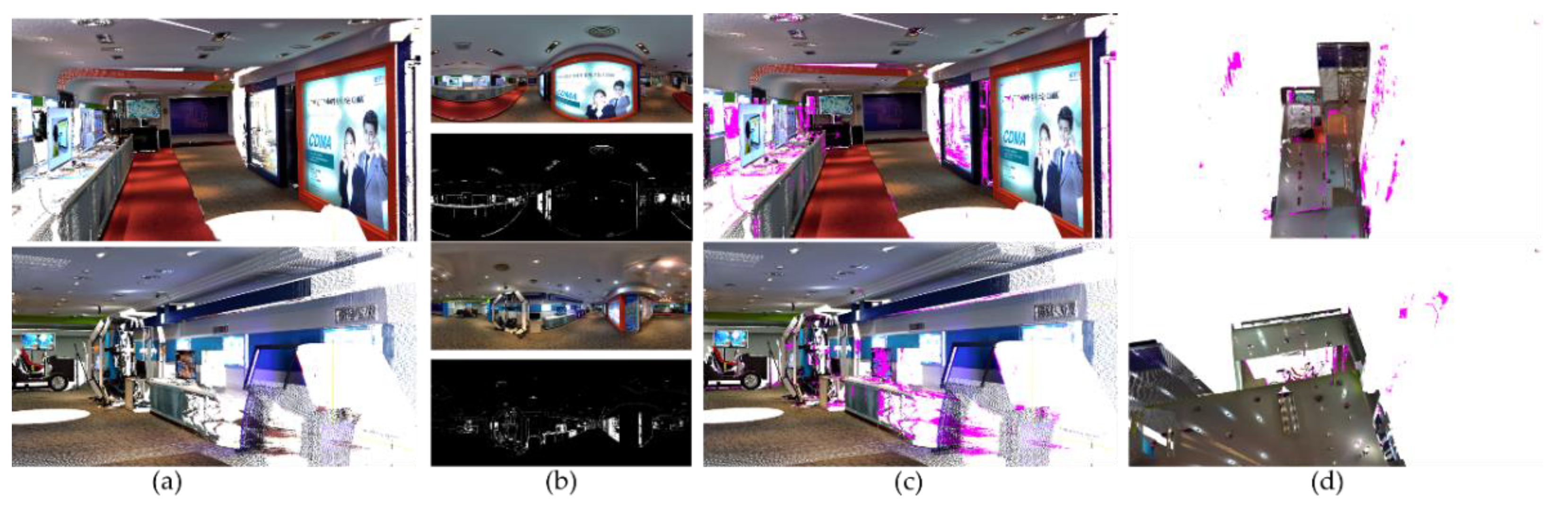
Overview of noise area. Part (a) is original point cloud view. The green part in (b) is the noise region detected by the method proposed in this paper. (c) is the RGB image in the same view. (d) is the point cloud after denoising by the method proposed in this paper.
Figure 2.
Overview of noise area. Part (a) is original point cloud view. The green part in (b) is the noise region detected by the method proposed in this paper. (c) is the RGB image in the same view. (d) is the point cloud after denoising by the method proposed in this paper.

Figure 3.
Overview of the proposed method.

Figure 4.
Reflective intensity value range image extract view.

Figure 5.
Range image-based noise detection module view.

Figure 6.
Transformer encoder view.

Figure 7.
Transformer decoder view.

Figure 8.
Noise detection results on individual sensor data. (a) Original point-cloud view; (b) RGB image from the LiDAR sensor and the 2D result image obtained by our method; (c) detected noise region (the purple part of the figure); (d) noise region from another view.
Figure 8.
Noise detection results on individual sensor data. (a) Original point-cloud view; (b) RGB image from the LiDAR sensor and the 2D result image obtained by our method; (c) detected noise region (the purple part of the figure); (d) noise region from another view.

Figure 9.
Comparison of the noise results. (a) is the original point cloud, (b) is the result after processing with FARO, (c) is the result obtained from the MPMC method, and (d) is the result obtained by our method.
Figure 9.
Comparison of the noise results. (a) is the original point cloud, (b) is the result after processing with FARO, (c) is the result obtained from the MPMC method, and (d) is the result obtained by our method.

Figure 10.
Results of the proposed method. (a) is the original point cloud, (b) shows the noise region detected by our method, highlighted in green, and (c) is the result of denoising using our method.
Figure 10.
Results of the proposed method. (a) is the original point cloud, (b) shows the noise region detected by our method, highlighted in green, and (c) is the result of denoising using our method.

Figure 11.
Results of the proposed method. (a) is the original point-cloud image, (b) the green part of the figure is the reflected noise region detected by our method, and (c) is the result obtained after denoising using our method.
Figure 11.
Results of the proposed method. (a) is the original point-cloud image, (b) the green part of the figure is the reflected noise region detected by our method, and (c) is the result obtained after denoising using our method.

Figure 12.
Results of the proposed method on another dataset. (a) is the original point cloud, (b) the green part of the figure is the noise region detected by our method, and (c) is the result of denoising using our method.
Figure 12.
Results of the proposed method on another dataset. (a) is the original point cloud, (b) the green part of the figure is the noise region detected by our method, and (c) is the result of denoising using our method.


Table 1.
Scanner setting parameters.
| Scanner Setting Name | Parameters |
|---|---|
| Scan Angular Area (Vertical) | |
| Scan Angular Area (Horizontal) | |
| Resolutions | 10,240 point/360 |
| Scanner Distance Range | 130 m |
| Horizontal Motor Speed Factor | 1.02 |
Table 2.
Point number of point clouds.
| Sensor Number | Total Number of Point Clouds | Total Number of Noise Points |
|---|---|---|
| S001 | 44,088,440 | 128,601 |
| S002 | 44,088,440 | 139,343 |
| S003 | 44,122,584 | 80,130 |
| S004 | 44,088,440 | 128,456 |
Table 3.
Point numbers of point clouds.
| Dataset Name | Point Cloud Number of a Single Scene/Object | The Total Number of Point Clouds | Scenes/Objects |
|---|---|---|---|
| PointCleanNet Dataset [24] | 100,000 | 2,800,000 | Objects |
| LS3DPC [35,36] | 857,142 | 6,000,000 | Scenes |
| Ours | 44,088,440 | 2,314,731,520 | Scenes |
Table 4.
Point numbers of point clouds.
| The Number of Point Cloud Data Points | |
|---|---|
| Train | 13 |
| Validation | 2 |
| Test | 4 |
| Total | 19 |
Table 5.
MPMC method and FARO SCENE filter parameters.
| Filter Name | Parameter Name | Parameters |
|---|---|---|
| MPMC [6] Method | Sliding window size | 100 |
| Stride | 50 | |
| 0.2 | ||
| 10,000 | ||
| Threshold of deletes nearest sensor γ | 4 | |
| Matching point threshold δ | 1 | |
| Nearest neighbor number ε | 8 | |
| Radius distance ζ | 0.01 | |
| FARO Dark Scan Point Filter | Reflectance Threshold | 900 |
| FARO Distance Filter | Minimum Distance | 0 |
| Maximum Distance | 200 | |
| FARO Stray Point Filter | Grid Size | 3 px |
| Distance Threshold | 0.02 | |
| Allocation Threshold | 50% |
Table 6.
Comparison of accuracy performance.
| Sensor Number | Accuracy (the Higher, the Better) | ||
|---|---|---|---|
| FARO [40] Result | MPMC [6] Result | Our Result | |
| S001 | 0.95351 | 0.94495 | 0.97139 |
| S002 | 0.93753 | 0.99058 | 0.98322 |
| S003 | 0.94718 | 0.96188 | 0.98905 |
| S004 | 0.95088 | 0.98981 | 0.99058 |
| Average | 0.94146 | 0.97181 | 0.98381 |
Table 7.
Comparison of the quantitative performance.
| Sensor Number | ODR | IDR | FPR | FNR | ||||||||
|---|---|---|---|---|---|---|---|---|---|---|---|---|
| FARO [40] Result | MPMC [6] Result | Our Result | FARO [40] Result | MPMC [6] Result | Our Result | FARO [40] Result | MPMC [6] Result | Our Result | FARO [40] Result | MPMC [6] Result | Our Result | |
| S001 | 0.1097 | 0.5870 | 0.7330 | 0.9710 | 0.9451 | 0.9726 | 0.0289 | 0.0548 | 0.0273 | 0.8902 | 0.4129 | 0.2669 |
| S002 | 0.1474 | 0.7947 | 0.7646 | 0.9835 | 0.9911 | 0.9926 | 0.0164 | 0.0088 | 0.0073 | 0.8525 | 0.2053 | 0.2353 |
| S003 | 0.1699 | 0.8102 | 0.8141 | 0.9558 | 0.9620 | 0.9780 | 0.0441 | 0.0379 | 0.0219 | 0.8300 | 0.1897 | 0.1858 |
| S004 | 0.1897 | 0.8413 | 0.8037 | 0.9399 | 0.9902 | 0.9939 | 0.0600 | 0.0097 | 0.0060 | 0.8102 | 0.1586 | 0.1962 |
| Average | 0.1542 | 0.7583 | 0.7788 | 0.9625 | 0.9721 | 0.9843 | 0.0374 | 0.0278 | 0.0156 | 0.8457 | 0.2416 | 0.2211 |
Table 8.
Computational resources comparison.
| Sensor Number | Memory (GB) | Time (Seconds) | ||||
|---|---|---|---|---|---|---|
| FARO [40] | MPMC [6] | Ours | FARO [40] | MPMC [6] | Ours | |
| S001 | 1.2 | 9.51 | 0.12 | 54.21 | 2362.42 | 743.41 |
| S002 | 2.6 | 13.49 | 1.86 | 113.65 | 4009.31 | 802.81 |
| S003 | 2.3 | 13.60 | 2.89 | 110.85 | 3552.80 | 874.48 |
| S004 | 2.4 | 13.59 | 2.89 | 114.72 | 4114.65 | 808.36 |
| Average | 2.125 | 12.52 | 1.25 | 98.35 | 3459.79 | 743.41 |
Publisher’s Note: MDPI stays neutral with regard to jurisdictional claims in published maps and institutional affiliations. |
© 2022 by the authors. Licensee MDPI, Basel, Switzerland. This article is an open access article distributed under the terms and conditions of the Creative Commons Attribution (CC BY) license (https://creativecommons.org/licenses/by/4.0/).
Share and Cite
MDPI and ACS Style
Gao, R.; Li, M.; Yang, S.-J.; Cho, K. Reflective Noise Filtering of Large-Scale Point Cloud Using Transformer. Remote Sens. 2022, 14, 577. https://0-doi-org.brum.beds.ac.uk/10.3390/rs14030577
AMA Style
Gao R, Li M, Yang S-J, Cho K. Reflective Noise Filtering of Large-Scale Point Cloud Using Transformer. Remote Sensing. 2022; 14(3):577. https://0-doi-org.brum.beds.ac.uk/10.3390/rs14030577
Chicago/Turabian StyleGao, Rui, Mengyu Li, Seung-Jun Yang, and Kyungeun Cho. 2022. "Reflective Noise Filtering of Large-Scale Point Cloud Using Transformer" Remote Sensing 14, no. 3: 577. https://0-doi-org.brum.beds.ac.uk/10.3390/rs14030577
Note that from the first issue of 2016, this journal uses article numbers instead of page numbers. See further details here.