
Experimental Study of Cloud-to-Ground Lightning Nowcasting with Multisource Data Based on a Video Prediction Method


Abstract
:1. Introduction
2. Data
2.1. Lightning Data
2.2. WRF Model Prediction Products
3. Method
3.1. Preprocessing of Lightning Data
3.2. Training Set and Test Set
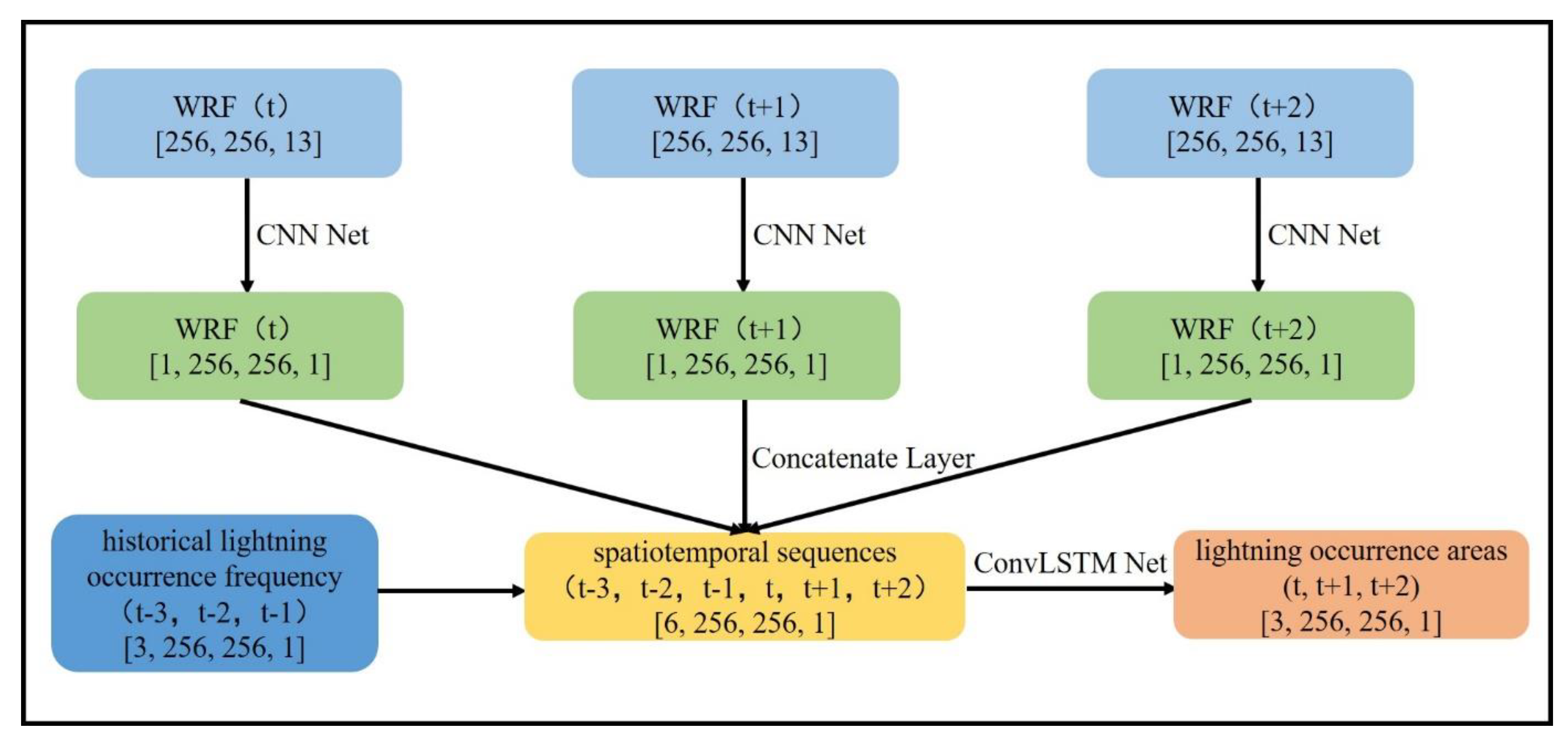
3.3. Neural Network Structure
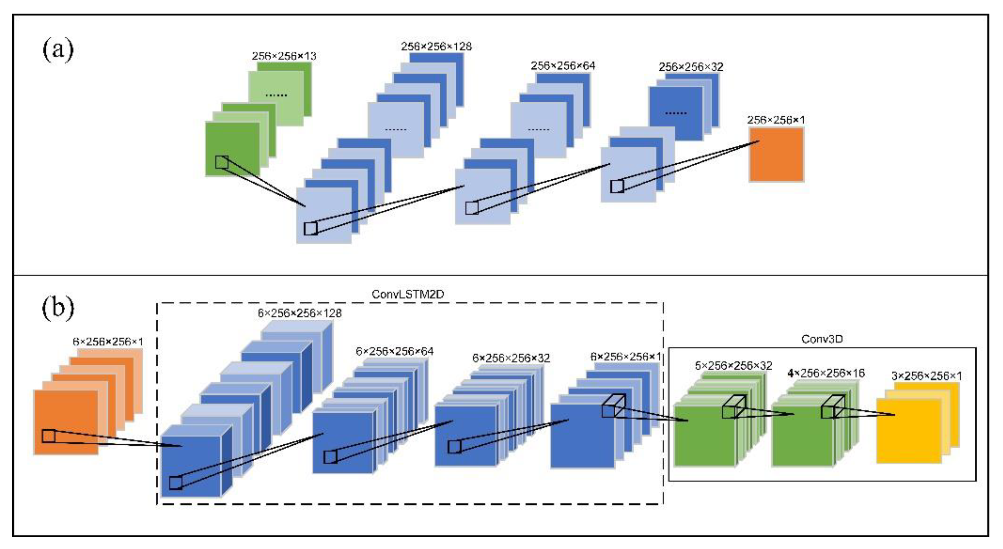
3.3.1. 2D and 3D Convolution Layers
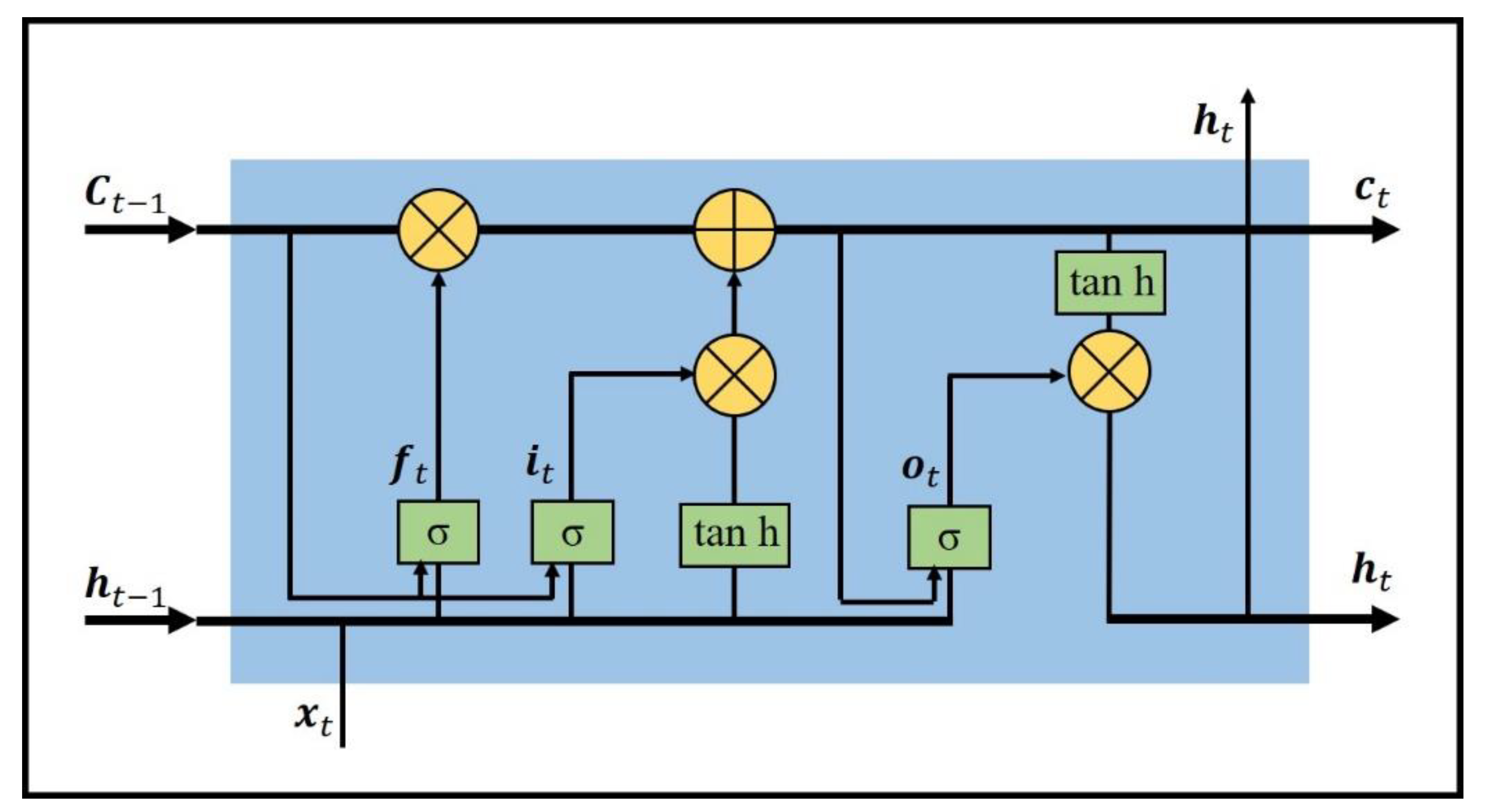
3.3.2. ConvLSTM
3.4. Network Training
3.5. Controlled Experimental Design
4. Forecast Results
4.1. Nowcasting Results and Scoring Test
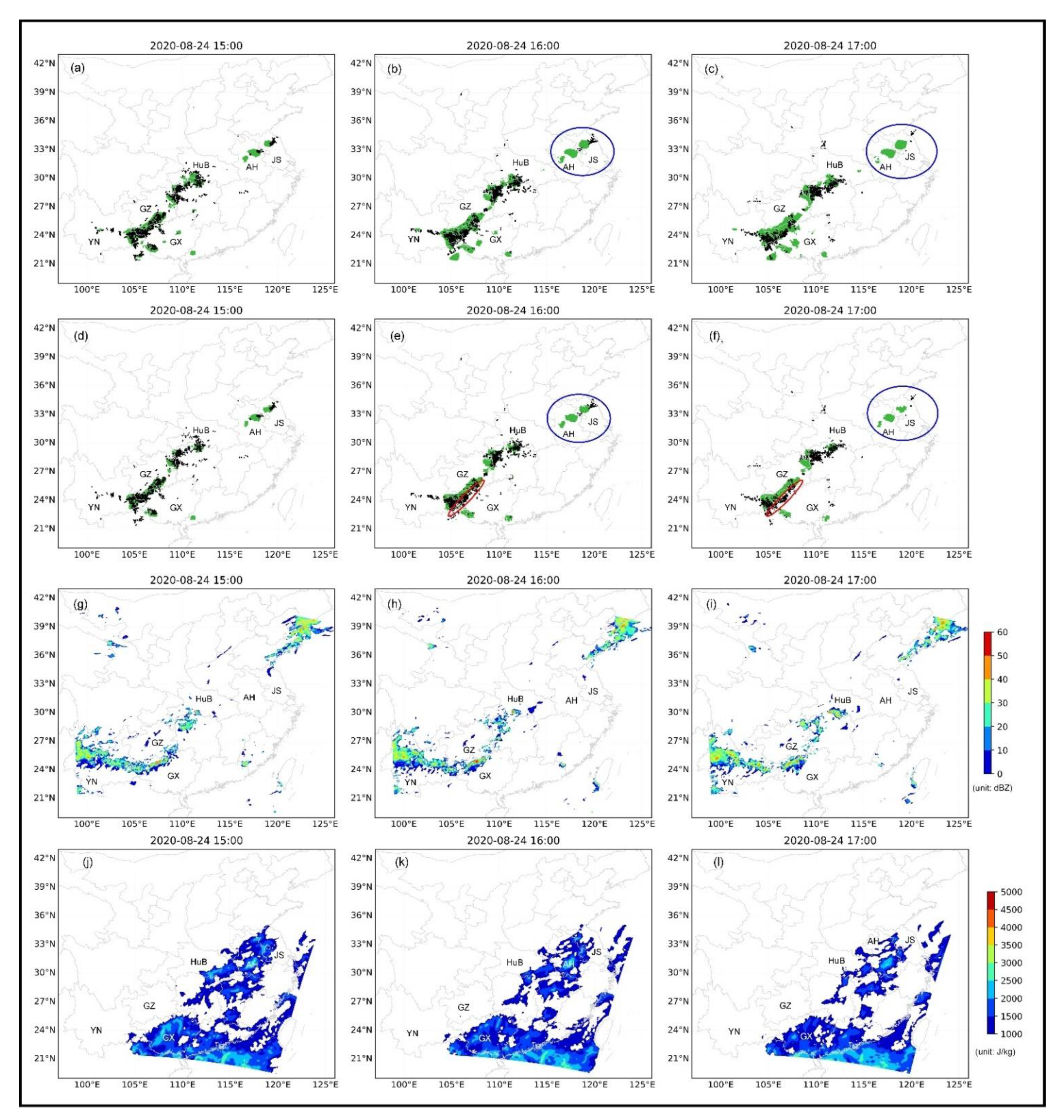
4.2. Case Study
5. Variable Importance Analysis
6. Conclusions
Author Contributions
Funding
Institutional Review Board Statement
Informed Consent Statement
Data Availability Statement
Acknowledgments
Conflicts of Interest
References
- Wilson, J.W.; Feng, Y.; Min, C.; Roberts, R.D. Nowcasting Challenges during the Beijing Olympics: Successes, Failures, and Implications for Future Nowcasting Systems. Weather. Forecast. 2010, 25, 1691–1714. [Google Scholar] [CrossRef]
- Wilson, J.W.; Crook, N.A.; Mueller, C.K.; Sun, J.; Dixon, M. Nowcasting Thunderstorms: A Status Report. Bull. Am. Meteorol. Soc. 1998, 79, 2079–2100. [Google Scholar] [CrossRef]
- Kuk, B.; Kim, H.; Ha, J.; Lee, H.; Lee, G. A Fuzzy Logic Method for Lightning Prediction Using Thermodynamic and Kinematic Parameters from Radio Sounding Observations in South Korea. Weather. Forecast. 2012, 27, 205–217. [Google Scholar] [CrossRef]
- Mazany, R.A.; Businger, S.; Gutman, S.I.; Roeder, W. A Lightning Prediction Index That Utilizes GPS Integrated Precipitable Water Vapor. Weather. Forecast. 2002, 17, 1034–1047. [Google Scholar] [CrossRef]
- Solomon, R.; Baker, M. Electrification of New Mexico Thunderstorms. Mon. Weather. Rev. 1994, 122, 1878–1886. [Google Scholar] [CrossRef] [Green Version]
- Brooks, H.E. Severe Thunderstorms and Climate Change. Atmos. Res. 2013, 123, 129–138. [Google Scholar] [CrossRef]
- Klazura, G.E.; Imy, D.A. A Description of the Initial Set of Analysis Products Available from the NEXRAD WSR-88D System. Bull. Am. Meteorol. Soc. 1993, 74, 1293–1312. [Google Scholar] [CrossRef] [Green Version]
- Dixon, M.; Wiener, G. TITAN: Thunderstorm Identification, Tracking, Analysis, and Nowcasting—A Radar-Based Methodology. J. Atmos. Ocean. Technol. 1993, 10, 785–797. [Google Scholar] [CrossRef]
- Vincent, B.R.; Carey, L.D.; Schneider, D.; Keeter, K.; Gonski, R. Using WSR-88D Reflectivity Data for the Prediction of Cloud-to-Ground Lightning: A Central North Carolina Study. Natl. Wea. Dig. 2004, 27, 35–44. [Google Scholar]
- Lang, T.J.; Rutledge, S.A. Relationships between Convective Storm Kinematics, Precipitation, and Lightning. Mon. Weather. Rev. 2002, 130, 2492–2506. [Google Scholar] [CrossRef]
- Martinez, M. The Relationship between Radar Reflectivity and Lightning Activity at Initial Stages of Convective Storms. In Proceedings of the American Meteorological Society, 82nd Annual Meeting, First Annual Student Conference, Orlando, FL, USA, 12–13 January 2002. [Google Scholar]
- Mosier, R.M.; Schumacher, C.; Orville, R.E.; Carey, L.D. Radar Nowcasting of Cloud-to-Ground Lightning over Houston, Texas. Weather. Forecast. 2011, 26, 199–212. [Google Scholar] [CrossRef]
- Hayashi, S.; Umehara, A.; Nagumo, N.; Ushio, T. The Relationship between Lightning Flash Rate and Ice-Related Volume Derived from Dual-Polarization Radar. Atmos. Res. 2021, 248, 105166. [Google Scholar] [CrossRef]
- Steiger, S.M.; Orville, R.E.; Carey, L.D. Total Lightning Signatures of Thunderstorm Intensity over North Texas. Part I: Supercells. Mon. Weather. Rev. 2007, 135, 3281–3302. [Google Scholar] [CrossRef]
- Price, C.; Rind, D. A Simple Lightning Parameterization for Calculating Global Lightning Distributions. J. Geophys. Res. Atmos. 1992, 97, 9919–9933. [Google Scholar] [CrossRef]
- Lynn, B.H.; Yair, Y.; Price, C.; Kelman, G.; Clark, A.J. Predicting Cloud-to-Ground and Intracloud Lightning in Weather Forecast Models. Weather. Forecast. 2012, 27, 1470–1488. [Google Scholar] [CrossRef]
- Wang, F.; Zhang, Y.; Dong, W. A Lightning Activity Forecast Scheme Developed for Summer Thunderstorms in South China. J. Meteorol. Res. 2010, 24, 631–640. [Google Scholar]
- Jayaratne, E.; Saunders, C.; Hallett, J. Laboratory Studies of the Charging of Soft-Hail during Ice Crystal Interactions. Q. J. R. Meteorol. Soc. 1983, 109, 609–630. [Google Scholar] [CrossRef]
- Saunders, C.; Keith, W.; Mitzeva, R. The Effect of Liquid Water on Thunderstorm Charging. J. Geophys. Res. Atmos. 1991, 96, 11007–11017. [Google Scholar] [CrossRef]
- Fierro, A.O.; Mansell, E.R.; MacGorman, D.R.; Ziegler, C.L. The Implementation of an Explicit Charging and Discharge Lightning Scheme within the WRF-ARW Model: Benchmark Simulations of a Continental Squall Line, a Tropical Cyclone, and a Winter Storm. Mon. Weather. Rev. 2013, 141, 2390–2415. [Google Scholar] [CrossRef]
- Xu, L.; Zhang, Y.; Wang, F.; Zheng, D. Coupling of Electrification and Discharge Processes with WRF Model and Its Preliminary Verification. Chin. J. Atmos. Sci. 2012, 36, 1041–1052. [Google Scholar]
- Sun, J.; Xue, M.; Wilson, J.W.; Zawadzki, I.; Ballard, S.P.; Onvlee-Hooimeyer, J.; Joe, P.; Barker, D.M.; Li, P.-W.; Golding, B.; et al. Use of NWP for Nowcasting Convective Precipitation: Recent Progress and Challenges. Bull. Am. Meteorol. Soc. 2014, 95, 409–426. [Google Scholar] [CrossRef] [Green Version]
- Badrinarayanan, V.; Kendall, A.; Cipolla, R. SegNet: A Deep Convolutional Encoder-Decoder Architecture for Image Segmentation. IEEE Trans. Pattern Anal. Mach. Intell. 2017, 39, 2481–2495. [Google Scholar] [CrossRef] [PubMed]
- Yuan, Z.; Zhou, X.; Yang, T. Hetero-Convlstm: A Deep Learning Approach to Traffic Accident Prediction on Heterogeneous Spatio-Temporal Data. In Proceedings of the 24th ACM SIGKDD International Conference on Knowledge Discovery & Data Mining, London, UK, 19–23 August 2018; pp. 984–992. [Google Scholar]
- Geng, Y.; Li, Q.; Lin, T.; Zhang, J.; Xu, L.; Yao, W.; Zheng, D.; Lyu, W.; Huang, H. A Heterogeneous Spatiotemporal Network for Lightning Prediction. In Proceedings of the 2020 IEEE International Conference on Data Mining (ICDM), Sorrento, Italy, 17–20 November 2020; pp. 1034–1039. [Google Scholar]
- Lin, T.; Li, Q.; Geng, Y.-A.; Jiang, L.; Xu, L.; Zheng, D.; Yao, W.; Lyu, W.; Zhang, Y. Attention-Based Dual-Source Spatiotemporal Neural Network for Lightning Forecast. IEEE Access 2019, 7, 158296–158307. [Google Scholar] [CrossRef]
- Zhou, K.; Zheng, Y.; Li, B.; Dong, W.; Zhang, X. Forecasting Different Types of Convective Weather: A Deep Learning Approach. J. Meteorol. Res. 2019, 33, 797–809. [Google Scholar] [CrossRef]
- Zhou, K.; Zheng, Y.; Dong, W.; Wang, T. A Deep Learning Network for Cloud-to-Ground Lightning Nowcasting with Multisource Data. J. Atmos. Ocean. Technol. 2020, 37, 927–942. [Google Scholar] [CrossRef]
- Oprea, S.; Martinez-Gonzalez, P.; Garcia-Garcia, A.; Castro-Vargas, J.A.; Orts-Escolano, S.; Garcia-Rodriguez, J.; Argyros, A. A Review on Deep Learning Techniques for Video Prediction. IEEE Trans. Pattern Anal. Mach. Intell. 2020. [Google Scholar] [CrossRef]
- Hu, A.; Cotter, F.; Mohan, N.; Gurau, C.; Kendall, A. Probabilistic Future Prediction for Video Scene Understanding. In Proceedings of the European Conference on Computer Vision, Glasgow, UK, 23–28 August 2020; pp. 767–785. [Google Scholar]
- Shi, X.; Chen, Z.; Wang, H.; Yeung, D.-Y.; Wong, W.-K.; Woo, W. Convolutional LSTM Network: A Machine Learning Approach for Precipitation Nowcasting. In Proceedings of the Advances in Neural Information Processing Systems, Montreal, QC, Canada, 7–12 December 2015; pp. 802–810. [Google Scholar]
- Shi, X.; Gao, Z.; Lausen, L.; Wang, H.; Yeung, D.-Y.; Wong, W.; WOO, W. Deep Learning for Precipitation Nowcasting: A Benchmark and A New Model. Adv. Neural Inf. Processing Syst. 2017, 30, 5617–5627. [Google Scholar]
- Yang, X.; Sun, J.; Li, W. An Analysis of Cloud-to-Ground Lightning in China during 2010–13. Weather. Forecast. 2015, 30, 1537–1550. [Google Scholar] [CrossRef]
- Xia, R.; Zhang, D.-L.; Wang, B. A 6-Yr Cloud-to-Ground Lightning Climatology and Its Relationship to Rainfall over Central and Eastern China. J. Appl. Meteorol. Climatol. 2015, 54, 2443–2460. [Google Scholar] [CrossRef]
- McCaul, W.E.; LaCasse, K.; Goodman, S. Use of High-Resolution WRF Simulations to Forecast Lightning Threat. In Proceedings of the 23rd Severe Storms Conference, St. Louis, MO, USA, 6–10 November 2006. [Google Scholar]
- Guerova, G.; Dimitrova, T.; Georgiev, S. Thunderstorm Classification Functions Based on Instability Indices and GNSS IWV for the Sofia Plain. Remote Sens. 2019, 11, 2988. [Google Scholar] [CrossRef] [Green Version]
- Yair, Y.; Lynn, B.; Price, C.; Kotroni, V.; Lagouvardos, K.; Morin, E.; Mugnai, A.; de Llasat, M.C. Predicting the Potential for Lightning Activity in Mediterranean Storms Based on the Weather Research and Forecasting (WRF) Model Dynamic and Microphysical Fields. J. Geophys. Res. Atmos. 2010, 115. [Google Scholar] [CrossRef] [Green Version]
- Chen, S.; Du, Y.; Fan, L.; He, H.; Zhong, D. A Lightning Location System in China: Its Performances and Applications. IEEE Trans. Electromagn. Compat. 2002, 44, 555–560. [Google Scholar] [CrossRef]
- Hu, M. Assimilation of Lightning Data Using Cloud Analysis within the Rapid Refresh. In Proceedings of the 4th Conference on the Meteorological Applications of Lightning Data, Phoenix, AZ, USA, 13 January 2009; American Meteorology Society: Boston, MA, USA, 2009; p. 29. [Google Scholar]
- Reap, R.M.; MacGorman, D.R. Cloud-to-Ground Lightning: Climatological Characteristics and Relationships to Model Fields, Radar Observations, and Severe Local Storms. Mon. Weather. Rev. 1989, 117, 518–535. [Google Scholar] [CrossRef]
- Dewan, A.; Ongee, E.T.; Rafiuddin, M.; Rahman, M.M.; Mahmood, R. Lightning Activity Associated with Precipitation and CAPE over Bangladesh. Int. J. Climatol. 2018, 38, 1649–1660. [Google Scholar] [CrossRef]
- Zheng, Y.; Chen, J.; Zhu, P. Climatological Distribution and Diurnal Variation of Mesoscale Convective Systems over China and Its Vicinity during Summer. Chin. Sci. Bull. 2008, 53, 1574–1586. [Google Scholar] [CrossRef] [Green Version]
- Howard, A.G. Some Improvements on Deep Convolutional Neural Network Based Image Classification. arXiv 2013, arXiv:1312.5402. [Google Scholar]
- Ratner, A.J.; Ehrenberg, H.R.; Hussain, Z.; Dunnmon, J.; Ré, C. Learning to Compose Domain-Specific Transformations for Data Augmentation. Adv. Neural Inf. Processing Syst. 2017, 30, 3239. [Google Scholar]
- Cubuk, E.D.; Zoph, B.; Mane, D.; Vasudevan, V.; Le, Q.V. AutoAugment: Learning Augmentation Policies from Data. arXiv 2019, arXiv:1805.09501. [Google Scholar]
- Nair, V.; Hinton, G. Rectified Linear Units Improve Restricted Boltzmann Machines Vinod Nair. In Proceedings of the ICML, Haifa, Israel, 21–24 June 2010; Volume 27, pp. 807–814. [Google Scholar]
- LeCun, Y.; Bottou, L.; Bengio, Y.; Haffner, P. Gradient-Based Learning Applied to Document Recognition. Proc. IEEE 1998, 86, 2278–2324. [Google Scholar] [CrossRef] [Green Version]
- Tivive, F.H.C.; Bouzerdown, A. An Eye Feature Detector Based on Convolutional Neural Network. In Proceedings of the Eighth International Symposium on Signal Processing and Its Applications, Sydney, Australia, 28–31 August 2005; Volume 1, pp. 90–93. [Google Scholar]
- Szarvas, M.; Yoshizawa, A.; Yamamoto, M.; Ogata, J. Pedestrian Detection with Convolutional Neural Networks. In Proceedings of the IEEE Intelligent Vehicles Symposium, Las Vegas, NE, USA, 6–8 June 2005; pp. 224–229. [Google Scholar]
- Muller, U.; Ben, J.; Cosatto, E.; Flepp, B.; Cun, Y.L. Off-Road Obstacle Avoidance through End-to-End Learning. In Proceedings of the Advances in Neural Information Processing Systems, Vancouver, BC, Canada, 4–5 December 2006; pp. 739–746. [Google Scholar]
- Lauer, F.; Suen, C.Y.; Bloch, G. A Trainable Feature Extractor for Handwritten Digit Recognition. Pattern Recognit. 2007, 40, 1816–1824. [Google Scholar] [CrossRef] [Green Version]
- Kingma, D.P.; Ba, J. Adam: A Method for Stochastic Optimization. arXiv 2017, arXiv:1412.6980. [Google Scholar]
- Buechler, D.E.; Goodman, S.J. Echo Size and Asymmetry: Impact on NEXRAD Storm Identification. J. Appl. Meteorol. Climatol. 1990, 29, 962–969. [Google Scholar] [CrossRef] [Green Version]
- Schaefer, J.T. The Critical Success Index as an Indicator of Warning Skill. Weather. Forecast. 1990, 5, 570–575. [Google Scholar] [CrossRef] [Green Version]
- Brownlee, K.A. Statistical Theory and Methodology in Science and Engineering; Wiley: Hoboken, NJ, USA, 1965. [Google Scholar]
- Roebber, P.J. Visualizing Multiple Measures of Forecast Quality. Weather. Forecast. 2009, 24, 601–608. [Google Scholar] [CrossRef] [Green Version]
- Breiman, L. Random Forests. Mach. Learn. 2001, 45, 5–32. [Google Scholar] [CrossRef] [Green Version]
- Zhou, K.; Zheng, Y.; Wang, T. Very Short-Range Lightning Forecasting with NWP and Observation Data: A Deep Learning Approach. Acta Meteorol. Sin. 2021, 79, 1–14. [Google Scholar] [CrossRef]
- Moncrieff, M.W.; Miller, M.J. The Dynamics and Simulation of Tropical Cumulonimbus and Squall Lines. Q. J. R. Meteorol. Soc. 1976, 102, 373–394. [Google Scholar] [CrossRef]
- Williams, E.R.; Geotis, S.; Renno, N.; Rutledge, S.; Rasmussen, E.; Rickenbach, T. A Radar and Electrical Study of Tropical “Hot Towers”. J. Atmos. Sci. 1992, 49, 1386–1395. [Google Scholar] [CrossRef] [Green Version]
- Wissmeier, U.; Goler, R. A Comparison of Tropical and Midlatitude Thunderstorm Evolution in Response to Wind Shear. J. Atmos. Sci. 2009, 66, 2385–2401. [Google Scholar] [CrossRef]
- Carey, L.D.; Rutledge, S.A. The Relationship between Precipitation and Lightning in Tropical Island Convection: A C-Band Polarimetric Radar Study. Mon. Weather. Rev. 2000, 128, 2687–2710. [Google Scholar] [CrossRef] [Green Version]
- Gauthier, M.L.; Petersen, W.A.; Carey, L.D.; Christian, H.J., Jr. Relationship between Cloud-to-Ground Lightning and Precipitation Ice Mass: A Radar Study over Houston. Geophys. Res. Lett. 2006, 33. [Google Scholar] [CrossRef]
- Sherwood, S.C.; Phillips, V.T.; Wettlaufer, J. Small Ice Crystals and the Climatology of Lightning. Geophys. Res. Lett. 2006, 33. [Google Scholar] [CrossRef] [Green Version]


| Variables | Description | Units |
|---|---|---|
| Wmax | maximum vertical velocity component of wind | m/s |
| helicity | storm relative helicity | m2/s2 |
| RAINNC | accumulated total grid scale precipitation | mm |
| QVAPOR | water vapor mixing ratio | g/kg |
| QCLOUD | cloud water mixing ratio | g/kg |
| QRAIN | rain water mixing ratio | g/kg |
| QICE | ice mixing ratio | g/kg |
| QSNOW | snow mixing ratio | g/kg |
| QGRAUP | graupel mixing ratio | g/kg |
| CAPE | convective available potential energy | J/kg |
| Rmax | maximum radar reflectivity | dBZ |
| R6 | radar reflectivity at 6 km above ground level | dBZ |
| R9 | radar reflectivity at 9 km above ground level | dBZ |
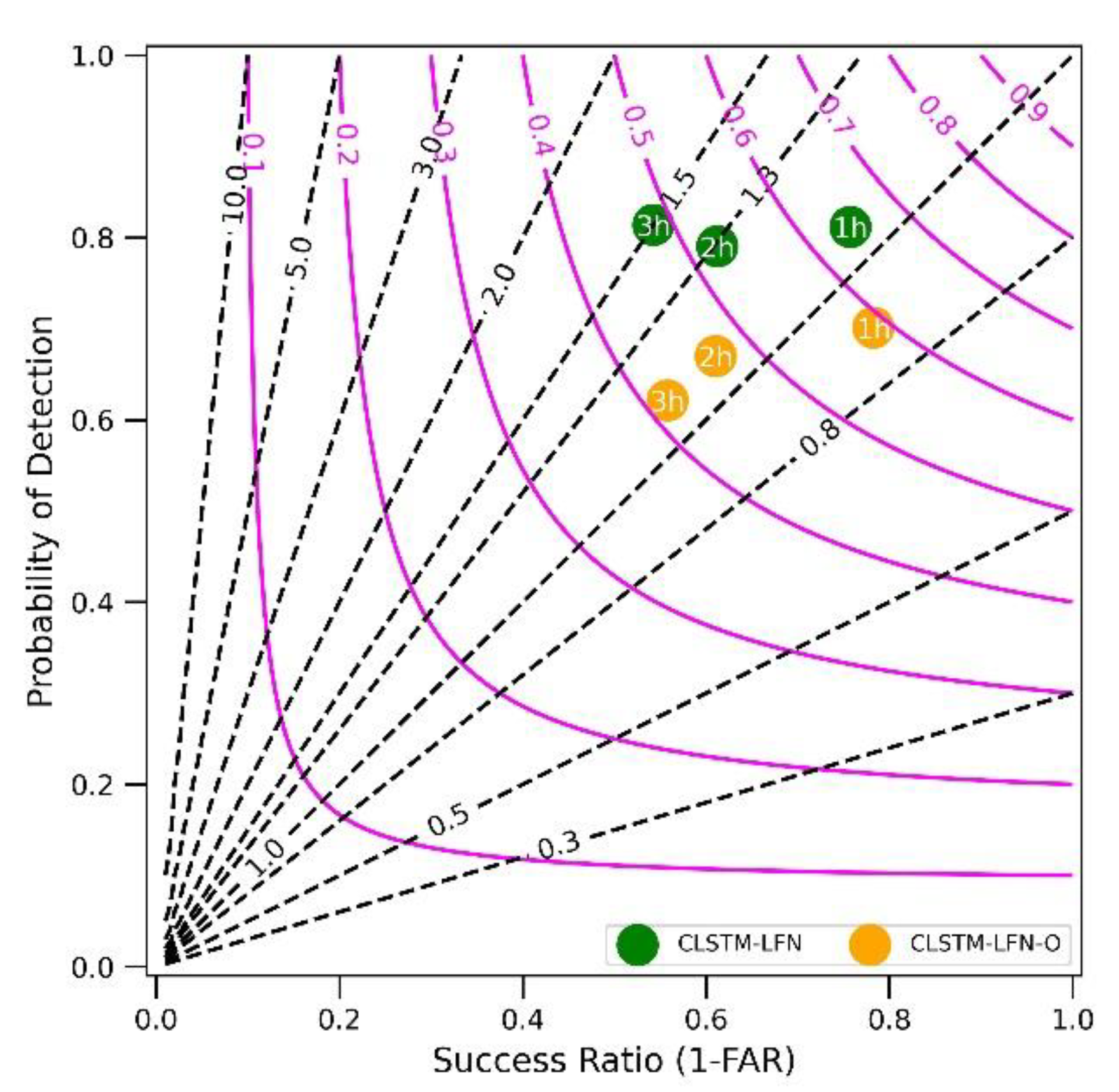
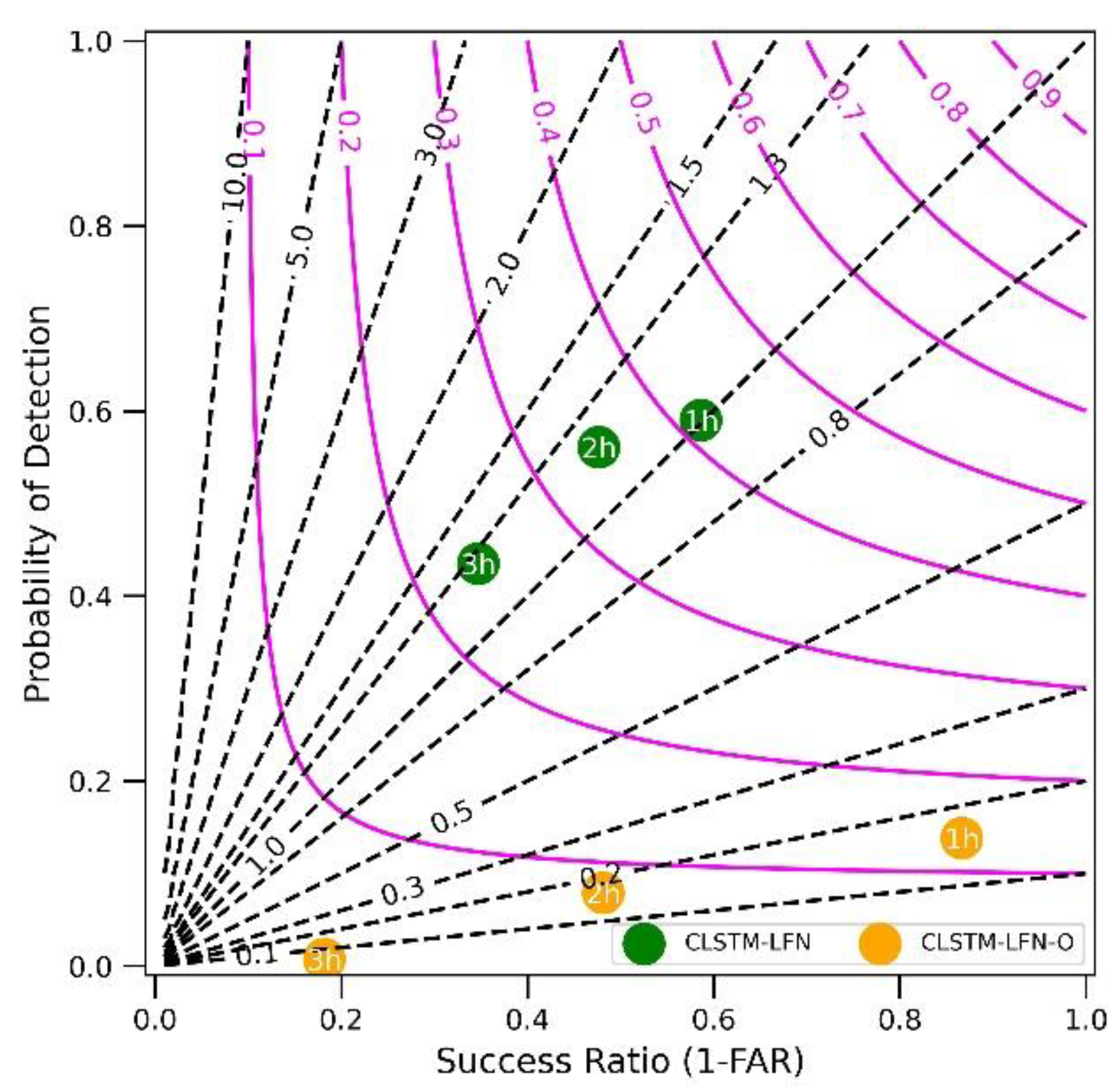
| Experiments | Forecast Time | TS | FAR | POD | Threshold (N) |
|---|---|---|---|---|---|
| CLSTM-LFN | 1 h | 0.518 | 0.367 | 0.741 | 5.0 |
| 2 h | 0.342 | 0.569 | 0.625 | ||
| 3 h | 0.240 | 0.693 | 0.523 | ||
| CLSTM-LFN-O | 1 h | 0.472 | 0.337 | 0.621 | 5.0 |
| 2 h | 0.325 | 0.552 | 0.544 | ||
| 3 h | 0.218 | 0.666 | 0.387 | ||
| CLSTM-LFN-W | 1 h | 0.114 | 0.869 | 0.467 | 2.0 |
| 2 h | 0.112 | 0.87 | 0.455 | ||
| 3 h | 0.105 | 0.873 | 0.382 | ||
| PR92 | 0–3 h | 0.053 | 0.94 | 0.304 | 0.0 |
| dBZ_from_WRF | 0–3 h | 0.007 | 0.869 | 0.007 | 0.0 |
Publisher’s Note: MDPI stays neutral with regard to jurisdictional claims in published maps and institutional affiliations. |
© 2022 by the authors. Licensee MDPI, Basel, Switzerland. This article is an open access article distributed under the terms and conditions of the Creative Commons Attribution (CC BY) license (https://creativecommons.org/licenses/by/4.0/).
Share and Cite
Guo, S.; Wang, J.; Gan, R.; Yang, Z.; Yang, Y. Experimental Study of Cloud-to-Ground Lightning Nowcasting with Multisource Data Based on a Video Prediction Method. Remote Sens. 2022, 14, 604. https://0-doi-org.brum.beds.ac.uk/10.3390/rs14030604
Guo S, Wang J, Gan R, Yang Z, Yang Y. Experimental Study of Cloud-to-Ground Lightning Nowcasting with Multisource Data Based on a Video Prediction Method. Remote Sensing. 2022; 14(3):604. https://0-doi-org.brum.beds.ac.uk/10.3390/rs14030604
Chicago/Turabian StyleGuo, Shuchang, Jinyan Wang, Ruhui Gan, Zhida Yang, and Yi Yang. 2022. "Experimental Study of Cloud-to-Ground Lightning Nowcasting with Multisource Data Based on a Video Prediction Method" Remote Sensing 14, no. 3: 604. https://0-doi-org.brum.beds.ac.uk/10.3390/rs14030604