
Multi-Exposure Image Fusion Techniques: A Comprehensive Review

Changchun Institute of Optics, Fine Mechanics and Physics, Chinese Academy of Sciences, Changchun 130033, China
*
Author to whom correspondence should be addressed.
Remote Sens. 2022, 14(3), 771; https://0-doi-org.brum.beds.ac.uk/10.3390/rs14030771
Submission received: 11 January 2022
/
Revised: 1 February 2022
/
Accepted: 1 February 2022
/
Published: 7 February 2022
(This article belongs to the Special Issue Multi-Task Deep Learning for Image Fusion and Segmentation)
Abstract
:Multi-exposure image fusion (MEF) is emerging as a research hotspot in the fields of image processing and computer vision, which can integrate images with multiple exposure levels into a full exposure image of high quality. It is an economical and effective way to improve the dynamic range of the imaging system and has broad application prospects. In recent years, with the further development of image representation theories such as multi-scale analysis and deep learning, significant progress has been achieved in this field. This paper comprehensively investigates the current research status of MEF methods. The relevant theories and key technologies for constructing MEF models are analyzed and categorized. The representative MEF methods in each category are introduced and summarized. Then, based on the multi-exposure image sequences in static and dynamic scenes, we present a comparative study for 18 representative MEF approaches using nine commonly used objective fusion metrics. Finally, the key issues of current MEF research are discussed, and a development trend for future research is put forward.
1. Introduction
Brightness in a natural scene usually varies greatly. For example, sunlight is about 105 cd/m2, room light is about 102 cd/m2, and starlight is about 10−3 cd/m2 [1]. Owing to the limitations of imaging devices, the dynamic range of a single image is much lower than that of a natural scene [2]. The shooting scene may be affected by light, weather, solar altitude, and other factors. Overexposure and underexposure often occur. A single image cannot fully reflect the light and dark levels of the scene, and some information may be lost, resulting in unsatisfactory imaging. Solving the problem of incomplete dynamic range matching in existing imaging equipment, display monitors, and the human eye’s dynamic response to real natural scenes is still challenging.
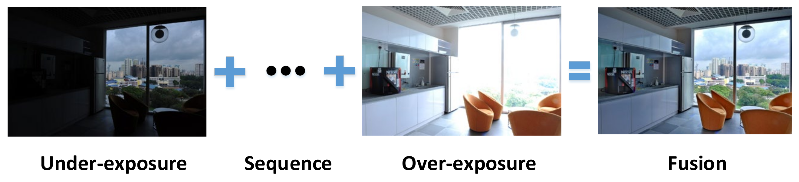
There are generally two ways to broaden the dynamic range of imaging detectors: hardware design and software technology. For the former, the CCD or CMOS detector needs to be redesigned, and a new optical modulation device may need to be introduced. Aggarwal [3] realized a camera design by dividing the aperture into multiple parts and using a set of mirrors to direct the light emitted by each piece to different directions. Tumblin [4] described a camera to measure the static gradient rather than static intensity and appropriately quantify the difference to capture HDR images. This kind of method can directly improve the efficiency of exposure quantity and imaging quality, but they are expensive and their practicability is limited. Through software technology, some researchers reconstruct the high dynamic range (HDR) image using the camera response function (CRF). Then, the HDR image can be displayed on the ordinary display device through tone mapping (TM). Others adopt MEF technology directly, fusing the input images with different exposure levels into an image with rich information and vivid colors, which do not need to consider camera curve calibration, HDR reconstruction, and tone mapping, as shown in Figure 1. Compared with the first way, MEF technology provides a simple, economical, and efficient manner to overcome the contradiction between HDR imaging and a low dynamic range (LDR) display. It avoids the complexity of imaging hardware circuit design and reduces the weight and power consumption of the whole device. It improves image quality and has essential application significance.
MEF is a branch of image fusion, similar to other image fusion tasks [5]; for example, multi-focus image fusion, visible and infrared image fusion, PET and MRI medical image fusion, multispectral and panchromatic remote sensing image fusion, hyperspectral and multispectral remote sensing image fusion, and optical and SAR remote sensing image fusion. They combine multidimensional content from multiple-source images to generate high-quality images containing more important information. The main difference between these image fusion tasks is that the source images are different, and the source images of MEF are a series of images with different exposure levels. In addition, it can also be used for image enhancement under low illumination [6,7], defogging [8], and saliency detection [9] by fusing or generating pseudo exposure sequences.
Research on MEF has been ongoing for more than 30 years, during which hundreds of relevant scientific articles have been published. In particular, with the continuous increase in the number and quality of newly proposed methods in recent years, significant progress has been achieved in this field [10]. A suitable MEF method should work stably in both static and dynamic scenes, appropriate exposure, good visual quality, and low consumption of computing cost, especially when processing high-resolution images. Therefore, the design of the MEF algorithm is a very challenging research task. This paper analyzes and discusses the research status and development trends of MEF technology. The main contributions of this review are summarized as follows.
1. The existing MEF methods are comprehensively reviewed. Following the latest developments in this field, the current MEF methods are divided into three categories: spatial domain methods, transform domain methods, and deep learning methods. The deghosting MEF methods in a dynamic scene are also discussed as a supplement and further analyzed.
2. A detailed performance evaluation is conducted. We compare the 18 representative MEF methods on multiple groups of typical source images using nine commonly used objective fusion metrics. The performance of MEF methods in static and dynamic scenes is analyzed. Relevant resources, including source images, fusion results, and related curves, have provided corresponding download links at “https://github.com/xfupup/MEF_data” (accessed on 9 January 2022). This is convenient for the comparison and analysis of the current MEF algorithms.
3. The challenges in the current study of MEF are discussed, and future research prospects are put forward.
2. A Review on MEF
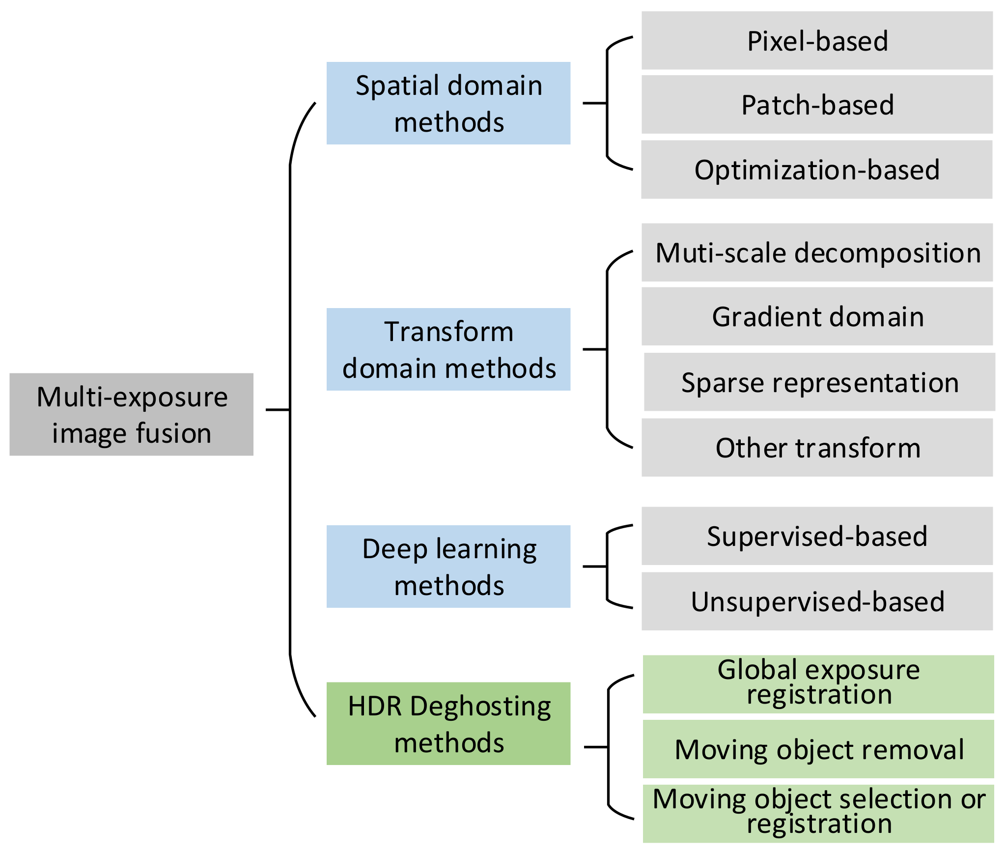
MEF has attracted extensive attention because it can effectively generate high-quality images with a high dynamic range by combining different information from the image sequence with different exposure levels. In the past 30 years, many scholars have proposed a variety of MEF algorithms. According to the existing research data, Burt et al. [11] were one of the earliest research teams to study MEF. In their work, a pyramid-based method was proposed to perform multiple image fusion tasks, including visible and infrared image fusion, multi-focus image fusion, and multi-exposure image fusion. After that, a large number of traditional MEF algorithms were proposed. In recent years, research based on deep learning has become a very active direction in MEF. The MEF algorithms can be classified in different ways. Zhang [10] divided MEF into three categories based on the number of input source images, whether the imaging scene is static or dynamic, and whether deep learning is used. Our research found that some methods can only process two images [10,12,13,14]. In [10], they compared the fusion results from the two images and gave a benchmark. However, most of the current MEF methods support multiple input images. Some MEF methods that can deal with the images in a static scene may also perform in a dynamic scene. Therefore, this paper presents a taxonomy of MEF methods that proposes to divide the existing MEF approaches into three categories: spatial domain methods, transform domain methods, and deep learning methods. In addition, MEF from a dynamic scene when camera jitters or moving objects are present has always been a challenge in this field. Ghost detection and elimination technology in a dynamic scene has already attracted much interest. This paper also further studies the MEF in a dynamic scene. The taxonomy is shown in Figure 2. It should be noted that although the presented taxonomy is valid in most cases, some hybrid algorithms are not easy to be classified into a single class. Such methods are classified according to their most dominant ideas.
The MEF methods based on the spatial domain use certain spatial features to fuse the input source images directly in the spatial domain according to specific rules. The general processing flow of this class of method is to generate a weight-mapping map for each input image and calculate the fused image as a weighted average of all input images. According to the level of information extraction, the MEF methods based on the spatial domain can be roughly divided into three types: pixel-based methods, patch-based methods, and optimization-based methods.
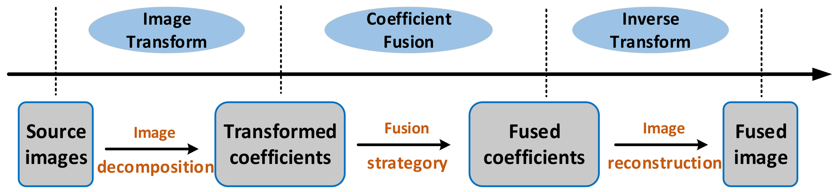
The MEF methods based on the transform domain generally consist of three stages: image transformation, coefficient fusion, and inverse transformation [15], as shown in Figure 3. First, the input images are transformed into another domain by applying image decomposition or image representation. Then, the transformed coefficients are fused through some pre-designed fusion rules. Finally, the fused image is reconstructed by the corresponding inverse transformation on the fused coefficients. Compared with the MEF methods based on spatial domain, the most prominent feature includes the inverse transformation stage of reconstructing the fused image. According to the transformation used, the MEF methods based on the transformation domain can be further divided into the multi-scale decomposition-based approaches, gradient-domain-based methods, sparse representation-based methods, and other transform-based methods.
In recent years, deep learning has become a very active direction in the field of MEF. Neural networks with a deep structure have been widely proved to have strong feature representation ability and are very useful for various image and vision tasks, including image fusion. Currently, deep learning models, including convolutional neural networks (CNNs) [16] and generative adversarial networks (GANs) [17], have been successfully applied to MEF. Depending on the model employed, deep learning-based methods can be further classified into supervised-based and unsupervised-based methods.
Due to the time difference in the image acquisition, camera jitter, and inconsistent object motion, it is challenging to avoid ghosts in fusion results [18,19]. The introduction of movement correction and relevant measures in the dynamic scene can effectively eliminate ghosts and improve the visual quality of the fused image. The deghosting algorithms in MEF can be broadly classified into three categories: global exposure registration, moving object removal, and moving object selection or registration.
Each category of the MEF methods is reviewed in detail as follows.
2.1. Spatial Domain Methods
2.1.1. Pixel-Based Methods
This kind of method directly fuses the pixel-based features of the source images according to certain fusion rules. Due to its advantages in obtaining accurate pixel weight maps for fusing, it has become a popular direction for MEF. These methods directly act on pixels. Most pixel-based methods are designed in the framework of a linear weighted sum, that is, the fused image is calculated as a weighted sum of all input images. The core problem is to obtain the weight map for each input image, and various pixel-based MEF methods have been proposed on different strategies to compute the weight maps. Bruce [20] normalized each pixel from the input image sequence and converted it into a logarithmic domain. Taking each pixel as the center and R as the radius, they calculated the entropy in the circle and assigned a weight to each pixel in line with the information entropy. Finally, the input images were merged based on the weight after exiting the logarithmic domain. Although the information entropy of the fused image is high, the color is unnatural in some cases. Lee [21] proposed an MEF method based on adaptive weight. Specifically, they defined two weight functions that reflected the pixel quality related to the overall brightness and global gradient. The final weight was the combination of these two weights. To adjust the brightness of the input images, Kinoshita [22] presented a scene segmentation method based on brightness distribution and tried to obtain the appropriate exposure values to decrease the saturation area of the fused image. Xu [23] designed a multi-scale MEF method based on physical features. In their work, a new Retinex model was used to obtain the illumination maps of the original input images, and weight maps were built, combined with the extracted features. Ulucan [24] introduced an MEF method based on linear embedding and watershed masking using a static scene. Linear embedding weights were extracted from differently exposed images. The corresponding watershed templates were used to adjust these mappings according to the information of the input images for the final fusion. However, the visual quality and statistical score will be reduced when the input image sequence contains extremely overexposed or underexposed images. There are many other pixel-level image fusion algorithms that use filtering methods to process the weighted maps. Raman and Chaudhuri [25] designed a bilateral filter-based MEF method that preserved the texture details of the input images at different exposure levels. Later, Li [26] used a median filter and recursive filter to reduce the noise of weight maps. However, only the gradient information of individual pixels was considered, regardless of the local regions.
The main drawback of pixel-based MEF methods is that they are sensitive to noise, ignore neighborhood information, and are prone to various artifacts in the final fused image. Therefore, most methods require some pre-processing, such as histogram equalization, or post-processing of the weight map, such as edge-preserving filtering, to produce a higher-quality fusion result. Even though the boundary filtering algorithms were added in some methods [25,26,27] and the halo artifacts can be reduced to some extent, the problem has not been solved at the root. Meanwhile, improvement strategies may bring new issues, such as breaking illumination relationships, over-relying on the bootstrap image, or significantly increasing computational complexity.
2.1.2. Patch-Based Methods
Unlike the pixel-based MEF method, the patch-based method divides the source images into multiple patch regions at a certain step size. Then, the patches at the same position corresponding to each image in the sequence are compared, and the patch containing the significant information is selected to form the final fused image. In [28], a patch-based method was first introduced to solve the MEF problem in the static scenes. The image was divided into uniform patches and the information entropy of each patch was used to measure the richness of the patch. They selected the most information patches and integrated them together using a patch-centered monotonically decreasing blending function to obtain the fused image. The disadvantage of this method is that it is easy to cause a halo at the boundary of different objects within the fused image. After that, many patch-based MEF methods were presented [29]. Ma [30] conducted a commonly used MEF method, which first extracted image patches from the input images, and decomposed them into three conceptually independent components: signal strength, signal structure, and average strength. These components were processed according to the patch intensity and exposure measurement to generate color image patches. These image patches were then put back into the fused image. Following this work, Ma [31] proposed a structural patch decomposition MEF approach (SPD-MEF). Compared with [30], the main improvement is that SPD-MEF can use the orientation of the signal structure components in the image patch to guide the verification of structural consistency for generating vivid images and overcoming ghost effects. This method does not need subsequent processing to improve visual quality or reduce spatial artifacts. However, the image patch size is fixed and has poor adaptability to the scene. The smaller size will cause the fused image to have serious spatial inconsistency, and the larger size will lead to the loss of detail in the fused image. On this basis, Li [32] proposed an improved multi-scale fast SPD-MEF method, which effectively reduced halo artifacts by recursively downsampling the patch size. In addition, the implicit implementation of structural patch decomposition also greatly improved the calculation efficiency. Later, Li [33] continued to add an edge detail retention factor and further designed a flexible bell curve for accurately estimating the weight function of the average intensity component. This function can retain the details in bright and dark regions and improve the fusion quality while maintaining a high computational speed. Wang [34] proposed an adaptive image patch segmentation method that used superpixel segmentation to divide the input images into non-overlapping patches composed of pixels with similar visual properties. Compared with the existing MEF methods that used fixed-size image patches, it avoided the patch effect and preserved the color properties of the source images.
In contrast to the pixel-based MEF methods, the main advantage of the approach based on patch is that the weight map has less noise because it combines the neighborhood information of the pixels and is robust to noise. However, since the patch in the image may span different objects, there are problems in edge detail retention, leading to edge blurring and halo, especially in edges with sharp changes in brightness.
2.1.3. Optimization-Based Methods
Several other MEF approaches are integrated into an optimization framework, and the weight maps are estimated by calculating the energy function. Shen [35] proposed a general random walk framework considering neighborhood information from the probability model and global optimization. The fusion was converted into a probabilistic estimation of the global optimal solution, and the computational complexity was reduced. However, since the method ultimately used a weighted average to fuse the pixels, it may degrade image details. In [2], by estimating the maximum a posteriori probability in the hierarchical multivariate Gaussian conditional random field, the optimal fusion weights can be obtained based on color saturation and local contrast. Li [36] performed MEF using fine detail enhancement for extracting the details from the input images based on quadratic optimization to improve the overall quality of the fused image. Song [37] approximated the ideal luminance image to a maximum contrast image using gradient constraints under the framework of maximum a posteriori probability. This fusion scheme integrated the gradient information of the input images and increased the fused image’s detail information. In [38], an underexposed image enhancement method was proposed, where the optimal weights were obtained by the energy function to retain the details and boost edges. Ma [39] obtained a fusion result by globally optimizing the structural similarity index that directly operated in all input images. They used the gradient rise optimization method to search the image to be optimized, which was the color MEF structural similarity (MEF-SSIMc) index, iteratively moving toward improving the MEF-SSIMc until convergence. The proposed optimization framework was easily extended when MEF models with better objective quality were available. In fused images, using only global optimization may lead to local overexposure or underexposure. Similarly, using only local optimization may degrade the overall performance of the fusion result. Therefore, Qi [40] combined a priori exposure quality and a structural consistency test to improve the robustness of MEF. At the same time, through the evaluation of exposure quality and the decomposition of image patch structure, the global and local quality of the fused image were optimized.
The main advantage of the optimization-based methods is that they are general. Specifically, they can flexibly change optimization indicators if a better one is available. However, this is also the major disadvantage of these methods, since a single indicator may not be sufficient to obtain a high-quality fused image. Therefore, the performance of these methods is highly indicator dependent. Unfortunately, there is no indicator that can completely express the fused image quality. All these methods suffer from severe artifacts such as ringing effects, loss of detail, and color distortion, which lead to poor fusion results. In addition, these methods are computationally intensive and cannot meet real-time requirements.
2.2. Transform Domain Methods
Transform domain-based MEF methods can be mainly classified into multi-scale decomposition-based methods, gradient domain-based methods, sparse representation based-methods, and other transform-based methods.
2.2.1. Multi-Scale Decomposition-Based Methods
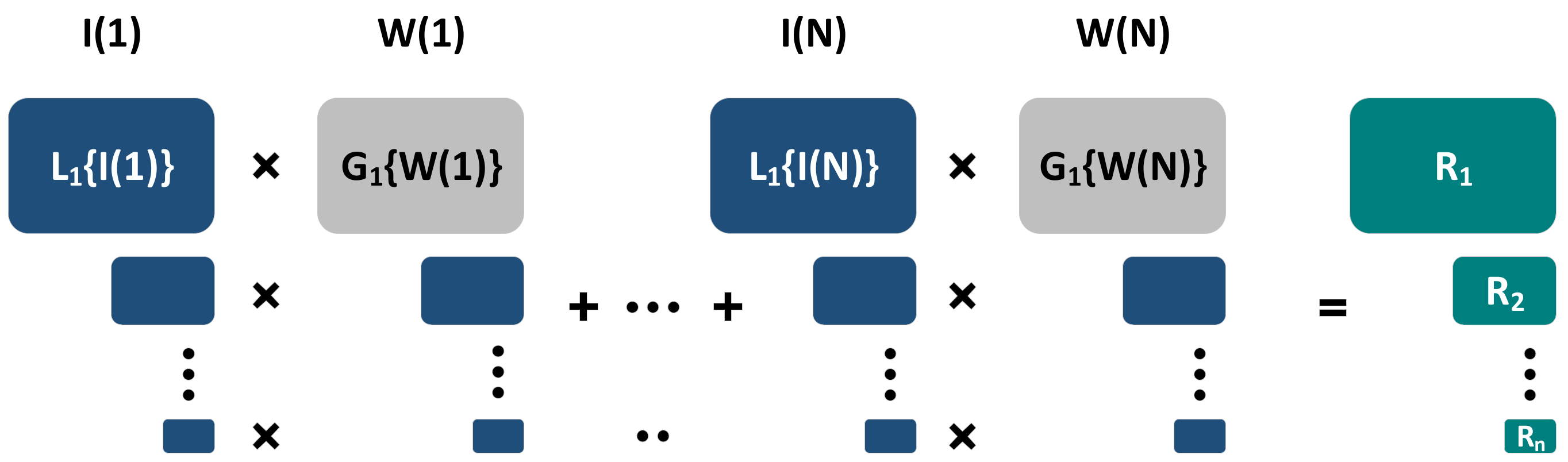
Burt [11] was one of the first to research the MEF algorithm, and proposed a gradient pyramid model based on directional filtering. Mertens [41] proposed a multi-scale fusion framework, as shown in Figure 4, which decomposed all the input images using the Laplace pyramid. The framework took the contrast, color saturation, and exposure to calculate and normalize the weight maps, which were smoothed by the Gaussian pyramid. Then, the Gaussian pyramid of the weight maps was multiplied by the Laplace pyramid of the multi exposure images to obtain the fusion result, which can better recover the image’s brightness, but cannot restore the details of the severely overexposed region. Based on this framework, many studies have been proposed to further improve fusion performance.
Li [42] presented a two-scale MEF method, which first decomposed the input images into base and detail layers and then calculated the weight maps by utilizing the significance measure. They fined weight maps using the guidance filter. The texture information of the input images could be retained, but halo artifacts still existed. An MEF method based on mixed weight and an improved Laplace pyramid was introduced to enhance the detail and color of the fused image in [43]. Based on the multi-scale guided filter, Singh [44] proposed an image fusion method to obtain detail-enhanced fusion images. This method had the advantages of both the multi-scale and guided filter methods, which can also be expanded in multi-focus image fusion task. Nejati [45] designed a fast MEF approach in which a guided filter was applied to decompose the input images for obtaining base and detail layers. To obtain the fused image, the brightness components of the input images were used to combine the base layers and the detail layers based on the blending weights of the exposure function. LZG [46] merged LDR images with different exposure levels by using the weighted guide filter to smooth the weight maps’ Gaussian pyramid. They designed a detail-extraction component to manipulate the details in the fusion image according to the users’ preference. Yan [47] proposed a simulated exposure model for white balance and image gradient processing. It integrated the input images under different exposure conditions into a fused image by using the linear fusion framework based on the Laplace pyramid. Wang [48] presented a multi-scale MEF algorithm based on YUV color space instead of RGB color space and designed a new weight smoothing pyramid used in YUV color space. A vector field construction algorithm was introduced to maintain the details of the brightest and the darkest areas in HDR scenes and avoid color distortion in the fused image. In some approaches, they often used edge-preserving smoothing technology to improve multi-scale MEF algorithms. Kou [49] proposed a multi-scale MEF method that introduced an edge-preserving smoothing pyramid to smooth the weight map. Owing to the edge-preserving characteristics of the filter, the details of the brightest/darkest regions in the fused image were well kept. Following [49], Yang [50] introduced a multi-scale MEF algorithm that first generated a virtual image with medium exposure based on the input images. Then, the method presented in [49] was applied to fuse this virtual image and achieve the fused result. Qu [51] proposed an improved Laplace pyramid fusion framework to achieve a fused image with detail enhancement. In addition, it is not easy to determine the appropriate fusion weight. To overcome this difficulty, Lin [52] presented an adaptive search strategy from coarse to fine, which used fuzzy logic and a multivariable normal conditional random field to search the optimal weight for multi-scale fusion.
2.2.2. Gradient-Based Methods
This kind of method is inspired by the physiological characteristics of the human visual system and is very sensitive to illumination. These methods aim to obtain the gradient information of the source images and then compose the fusion image in the gradient domain. Gu [53] presented an MEF method in a gradient field based on Riemannian geometric measurement and the gradient value of each pixel, which was generated by maximizing the structure tensor. The final fused image was obtained by a Poisson solver. The average gradient of the fused image was high, and this method was suitable in the details. However, the color was rarely processed, such that the fused image was dark, and the color was unnatural. Zhang [54] proposed an MEF method to apply in static and dynamic scenes based on gradient information. Under the guidance of the gradient-based quality evaluation, it generated a tone map similar to a high dynamic range image through seamless synthesis. Similarly, research using the gradient-based method to maintain image saliency was presented in [55], where the significance gradient of each color channel was computed. Moreover, the acquisition of the gradient was also a critical issue for calculating the image contrast. In general, the corresponding eigenvector of the matrix decided the gradient amplitude of the fusion. Several improved approaches were appropriated to optimize the weighted sum of the gradient amplitude in [56]. In this method, they used a wavelet filter, decomposing the image luminance, to obtain the corresponding decomposition coefficients. Paul [57] designed an MEF approach based on the gradient domain, which first converted the input images into YCbCr color space and then performed the fusion of the Y channel in the gradient domain. At the same time, the chrominance channels (Cb and Cr) were fused by applying a weighted sum of the chrominance channels. Specifically, the gradient in each orientation was estimated based on the maximum amplitude gradient selection. Using the gradient, the luminance was reconstructed based on the Harr wavelet. In [58], according to local contrast, brightness, and spatial structure, the author first calculated three weights of the input images and combined them using the multi-scale Laplacian pyramid. The dense scale-invariant feature transformation was used to compute the local contrast around each pixel position and measure the weight maps. The luminance was calculated in the gradient domain to obtain more visual information.
2.2.3. Sparse Representation-Based Methods
The approaches based on sparse representation (SR) take the linear combination of elements in the over-complete dictionary to describe the input signal. The error between the reconstructed signal and the input signal is minimized with as few non-zero coefficients as possible, allowing for a more concise representation of the signal and easier access to signal details [59]. In the past decade, SR-based MEF methods have rapidly become an essential branch in the area of image fusion. A dictionary obtained by K-SVD was used to represent the overlapping patches of the image brightness by the “sliding window” technique in [60]. The fusion image was reconstructed based on the sparse coefficients and the dictionary. Shao [61] proposed a local gradient sparse descriptor to generate the local details of the input image. It extracted the image features to remove the halo artifacts when the brightness of the source images changed sharply. Yang [62] designed a sparse exposure dictionary for exposure estimation based on sparse decomposition, which was used to construct the exposure estimation maps according to the atomic number of the image patches obtained by sparse decomposition.
2.2.4. Other Transform-Based Methods
In addition to the above methods, discrete cosine transform (DCT) and wavelet transform have also been successfully applied to MEF. Lee [63] proposed an HDR enhancement method based on DCT that fused two overexposure and underexposure images. This algorithm used the quantization process in JPEG coding as a metric for improving image quality so that the fusion process can be included in the DCT-based compression baseline. They proposed a Gaussian error function based on camera characteristics to improve the global image brightness. Martorell [64] constructed an MEF method based on the sliding window DCT transform, which used YCbCr transform to calculate the luminance and chrominance components of the image, respectively. Specifically, this technique decomposed the input images into multiple patches and computed the DCT of these patches. The patch coefficients from the same position of the input images with different exposure levels were combined according to their sizes. The chromaticity values were fused separately as a weighted average at the pixel level. In [65], the input images were converted into YUV space, and the color difference components U and V were fused in line with the saturation weight. The luminance component Y was converted into the wavelet domain, and the corresponding approximate sub-band and detail sub-band were fused by the well-exposedness weight and adjustable contrast weight, respectively. The final fused result was obtained by transforming the fusion image into RGB space.
2.3. Deep Learning Methods
In recent years, significant success has been achieved based on deep learning in computer vision and image processing applications [66,67]. More and more MEF methods based on deep learning have been proposed to improve fusion performance [68,69,70,71]. To provide some useful references for researchers, the achievements in recent years based on deep learning are reviewed, including supervised and unsupervised MEF methods.
2.3.1. Supervised Methods
In supervised MEF algorithms, a large number of multi-exposure images with ground truth are required for training. However, this requirement is difficult to meet because there is generally no ground truth available in the MEF. Researchers have to find effective ways to create ground truth to develop this kind of method. CNN is known to be effective to learn local patterns and capture promising semantic information. Furthermore, it is also known to be efficient compared with other networks [72,73]. In 2017, Kalantari [74] first introduced a supervised CNN framework for MEF research. The ground truth image dataset was generated by combining three static images with different exposure levels in their work. The three images were converted into an approximate static scene by optical flow. Then, a convolutional neural network (CNN) was used to obtain fusion weights and fuse the aligned images. The contributions of this paper were: (1) presenting the first study on deep learning MEF; (2) the fusion effects of the three CNN architectures were discussed and compared; and (3) a dataset suitable for MEF was created. Since then, many MEF algorithms based on deep learning have been proposed. In 2018, Wang [75] proposed a supervised CNN-based framework for MEF. The main innovation of the approach was that it used the CNN model to gain multiple sub-images of the input images to use more neighborhood information for convolution operation. This work changed the pixel intensity of the ILSVRC 2012 verification dataset [76] to generate the ground truth images. However, it may not be real for the ground truth images generated in this way.
The second way to solve the lack of the ground truth is to use the pre-trained model generated by different methods. Li [77] extracted the features of the input images by utilizing a pre-trained model in other networks and calculated the local consistency using these features to determine the weights. In addition, due to motion detection implementation, this method can be used in both static and dynamic scenes. Similar work was also presented in [78].
The third way to solve this problem is to select fusion results from some methods as the ground truth. Cai [79] used 13 representative MEF techniques to generate 13 corresponding fused images from each sequence and then selected the image with the best visual quality as the ground truth by conducting subjective experiments. They provided a dataset containing 589 groups of multi-exposure image sequences, with 4413 images. The whole process required much manual intervention, so the number of image sequences trained was very limited, which may hinder the generalization ability of the fusion network. Liu [80] proposed a network for decolorization and MEF based on CNN. To obtain satisfactory qualitative and quantitative fusion results, the local gradient information from the input images with different exposure levels was calculated as the network’s input. It worked on a source image sequence consisting of three exposure levels and each exposure level can be viewed as a signal channel. In [81], a dual-network cascade model was constructed consisting of an exposure prediction network and an exposure fusion network. The former was used to recover the lost details in underexposed or overexposed regions, and the latter could perform fusion enhancement. This cascade model used a three-stage training strategy to reduce the training complexity. However, the down-sampling operation in this model may cause checkerboard defects in the fused image, and the author alleviated this problem by applying a loss function constructed with the structural anisotropy index.
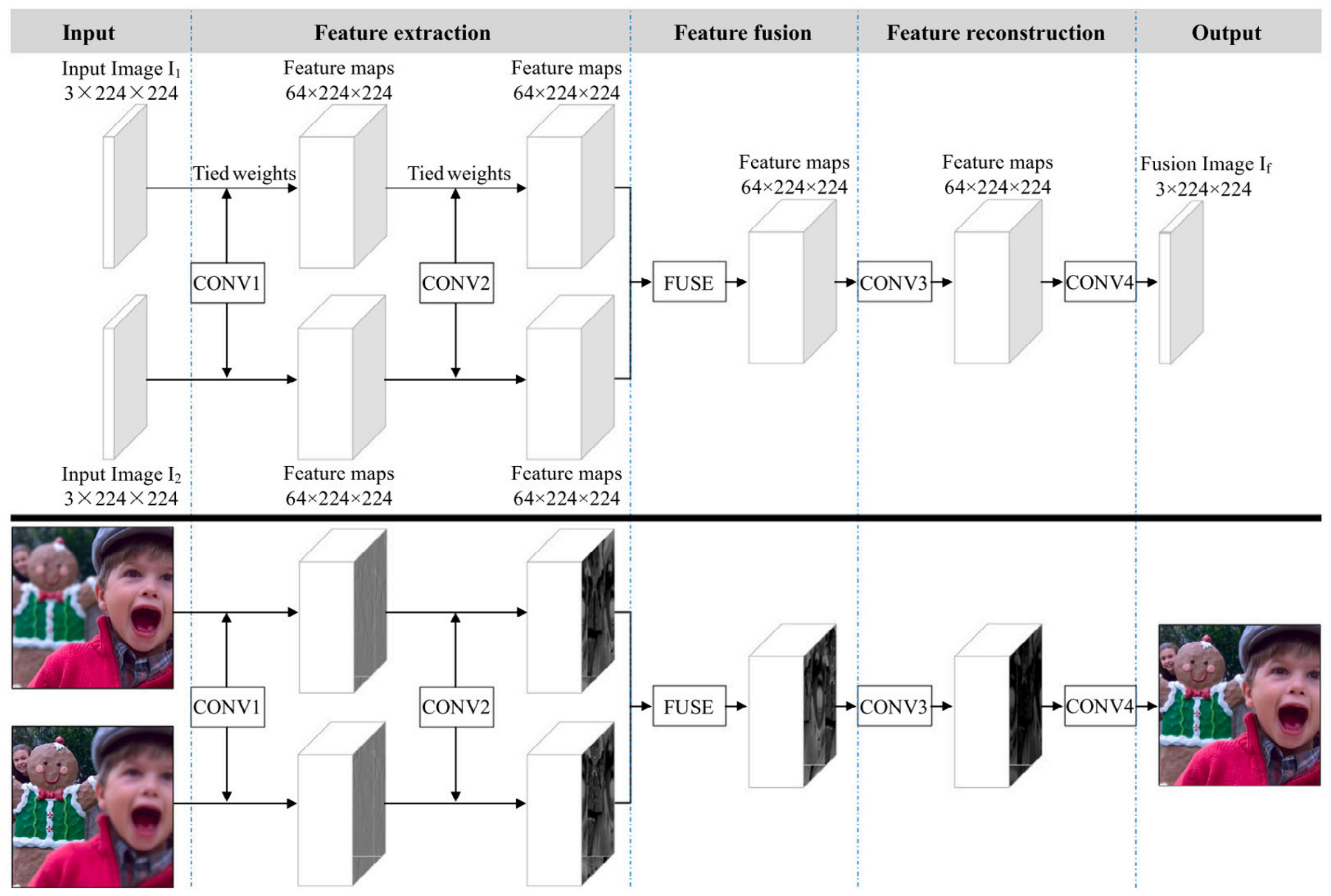
The above supervised methods are explicitly designed for the MEF issue. There are also several methods based on supervised deep learning that are constructed for some image fusion tasks, including MEF. Zhang [82] proposed an end-to-end fully convolutional approach (IFCNN) that used Siam architecture, as shown in Figure 5. Two branches extracted the convolutional features from the input images and fused them using element average fusion rules (note that different fusion tasks used different rules). In IFCNN, the model was optimized utilizing perceptual loss, plus a fundamental loss that calculated the intensity difference between the input images and the ground truth. IFCNN can be suitable for fusing images at arbitrary resolution. However, its performance in the MEF task may be limited because it was trained only with a multi-focus image dataset. In [83], a general cross-modal image fusion network was presented, exploring the commonalities and characteristics of different fusion tasks. Different network structures were analyzed in terms of their impact on the quality and efficiency of image fusion. The dataset constructed by Cai [79] was used for the MEF task. However, these models were not explicitly designed for MEF issues and were not fine-tuned on multi-exposure images, so their performance may not be satisfactory in some cases.
The methods above either create the ground truth images by adjusting the brightness value of the normal images, use other pre-trained models in other works to obtain the ground truth images, or use the images with subjective effects in the existing fusion results as the ground truth images. However, these methods may not deal well with the lack of real ground truth images. In particular, the ground truth images in some MEF algorithms are selected from the fusion results of other methods and not taken by optical cameras. They may not be accurate or appropriate. In order to solve these problems, some studies try to construct unsupervised MEF architectures.
2.3.2. Unsupervised Methods
Since there are generally no real ground truth images available, some studies have turned to developing the MEF methods based on unsupervised deep learning to avoid the need for ground truth in training. This section describes the relevant unsupervised MEF methods.
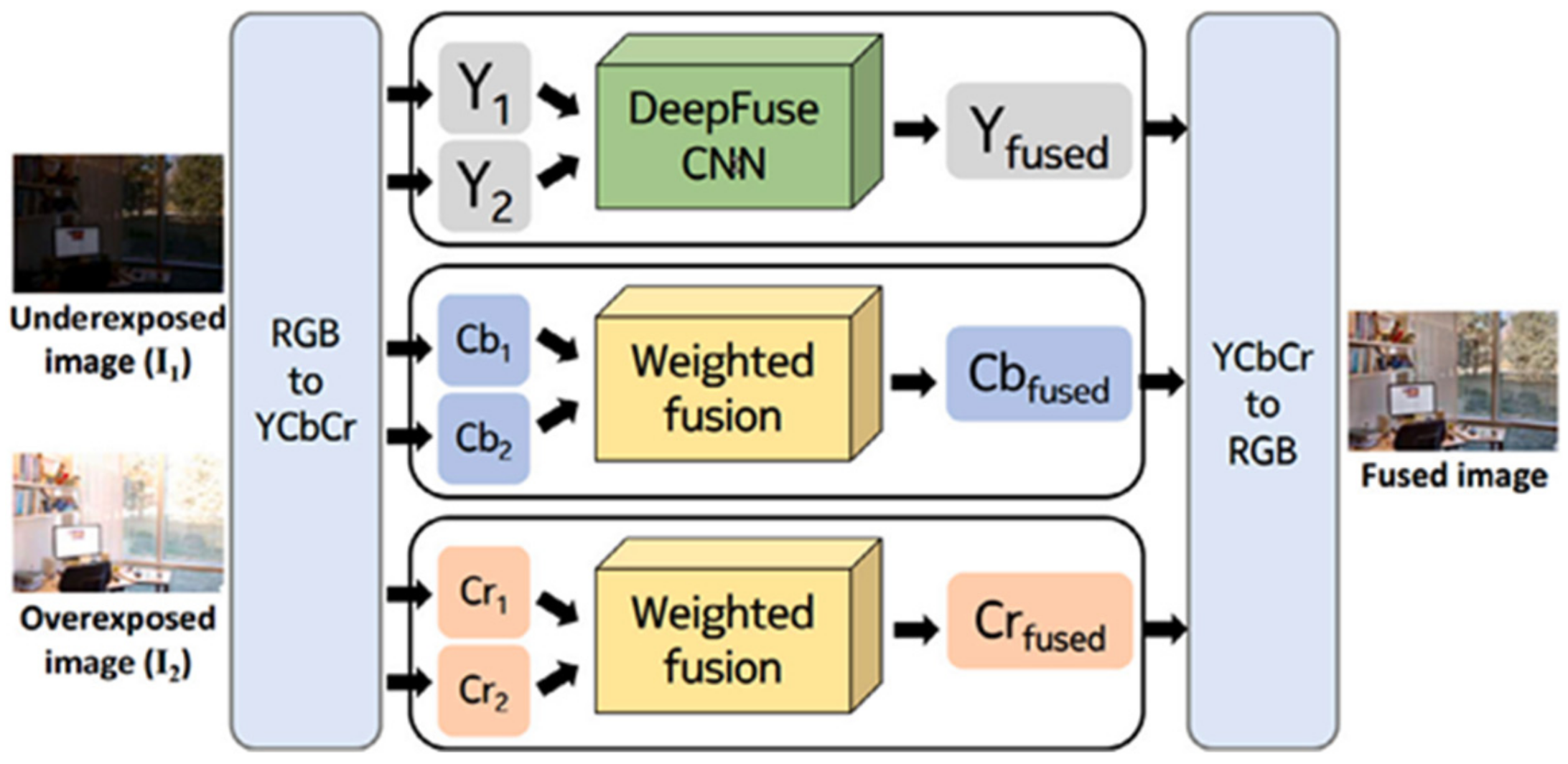
In 2017, Prabhakar [84] built the first unsupervised MEF architecture for fusing image pairs, named DeepFuse, as shown in Figure 6. This method first converted the input images into YCbCr color space. Then, a CNN composed of the feature layers, a fusion layer, and the reconstruction layers was used for feature extraction of the Y channel, while the fusion of Chrominance channels (Cb and Cr) was still executed manually. Thirdly, the image data in YCbCr space were converted back into RGB space to obtain the final fusion image. This unsupervised method used a fusion quality metric MEF-SSIM [85] as the loss function to realize unsupervised learning. DeepFuse can extract effective features and be more robust to different inputs because it uses CNN to fuse the brightness, which is its main advantage. Furthermore, as an unsupervised method, it does not need ground truth to train. However, a different color space conversion is required, which is not easy compared with fusing RGB images directly. In addition, simply using MEF-SSIM as the loss function is not enough to learn other critical information not covered by MEF-SSIM.
Ma [86] presented a flexible and fast MEFNet for the MEF task, and it also worked in the YCbCr color space. First, the input images were downsampled and sent to a context aggregation network for generating the learned weight maps, which were jointly upsampled to high resolution using a guided filter. Then, the upsampling weight maps were used for the weighted summation of the input images. Specifically, the context aggregation network was trained for fusing the Y channel, while the fusion of Cb and Cr was executed with a simple weighted summation. The final fused image in RGB space was obtained by converting color space. The flexibility and speed were the significant advantages of MEFNet, i.e., the input images with arbitrary spatial resolution can be fused using this fully convolutional network, and the fusion process was efficient since the main calculation was carried out with a fixed low resolution. However, because only MEF-SSIM was used as the loss function, there was the same problem in MEFNet as in DeepFuse.
Qi [87] presented the UMEF network for MEF in static scenes. They used CNN to extract features and fused them to create the final fusion image. Compared with DeepFuse, there were three main differences between them, as follows. First, UMEF can fuse multiple input images. By contrast, DeepFuse was designed to fuse two input images. Second, the loss function was made up of two parts: MEF-SSIMc and an unreferenced gradient loss, while the loss function of DeepFuse was only MEF-SSIM. As a result, more details of the fused images were reserved in UMEF. Third, the color images can be directly fused with MEF-SSIMc in UMEF, and the color space conversion is avoided. In [88], an end-to-end unsupervised fusion network was designed to generate a fusion image, named U2Fusion. It was applied to solve different fusion tasks, such as multi-modal, multi-exposure, and multi-focus issues. U2Fusion extracted the features with pre-trained VGGNet-16 and fused the input images with the DenseNet network. The importance of the input images can be automatically estimated through feature extraction and information measurement, and an adaptive information preservation degree was put forward. However, this method was required for the quality of the input images. When acquiring the image, these problems will be amplified if there is noise or distortion. Gao [89] made some improvements based on U2Fusion and applied the MEF model to the transportation field. The quality of the fused images from the fusion model was improved using adaptive optimization.
Besides the unsupervised method based on CNN, some unsupervised MEF methods based on Generative Adversarial Networks (GAN) were also proposed. Chen [90] presented an MEF network and fused two input images. This network integrated homography estimation, attention mechanism, and adversarial learning, which were, respectively, applied to camera motion compensation, the correction of the remaining moving pixels, and artifact reduction. Xu [17] designed an end-to-end architecture for MEF based on GAN, named MEF-GAN, and used the dataset from Cai [79]. Following [17] and [90], a GAN-based MEF network, named GANFuse, was proposed in [91]. There were two main differences between GANFuse and the GAN-based MEF approaches above. First, as an unsupervised network, GANFuse used an unsupervised loss function, which was applied to measure the similarity between the fusion image and the input images, rather than the similarity with the ground truth. Second, GANFuse was composed of one generator and two discriminators. Each discriminator was used to distinguish the difference between the fusion image and the input images.
It should be noted that all the above unsupervised MEF networks, except UMEF, required color space conversion. The input images needed to be converted into YCbCr color space, and the Y channel was fused with the deep learning model, while the Cb and Cr channels were fused by weighted summation.
2.4. HDR Deghosting Methods
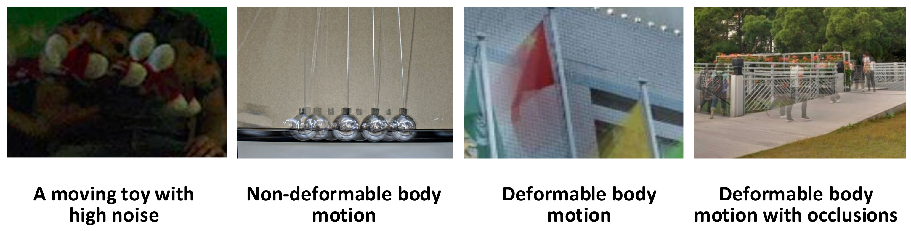
Most MEF approaches assume that the source images are perfectly aligned, which is usually violated in practice because of the time differences in image acquisition. Once there are moving objects in the scene, ghosts or blur artifacts often occur that degrade the quality of the fusion image [92,93,94], as shown in Figure 7.
MEF in dynamic scenes has always been a challenge. To obtain HDR images without artifacts, a large number of deghosting MEF methods have been proposed from different angles, which are mainly in two aspects: how to detect the ghost area and how to eliminate ghosts. Based on the above parts, this part analyzes the MEF deghosting methods in-depth. The current MEF methods in dynamic scenes are investigated, classified, and compared. The MEF processing in a dynamic scene is divided into the following categories: global exposure registration, moving object removal, and moving object selection or registration.
2.4.1. Global Exposure Registration
The main aim of the methods in this class is to compensate for and eliminate the impacts of the camera motion based on parameter estimation of the transformations that are applied to each input image. These methods do not pay attention to the existence of moving objects.
Cerman [95] presented an MEF approach to register the source images and eliminate the camera motion in handheld image acquisition equipment. The correlation in the Fourier domain was used to evaluate the image offset from the translational camera motion in initial estimation. Both the translational and rotational movement of the subpixels between input images were locally optimized. They used the registration on continuous image pairs without selecting a reference image. Gevrekci [96] proposed a new contrast-invariant feature transform method. This method assumed that the Fourier components were in phase at the corner position, used a local contrast stretching step on each pixel of the source images, and applied the phase congruency for detecting the corners. Then, they registered the source images by matching features using RANSAC. Another approach using the phase congruency images was provided in [97], which used cross-correlation technology to register the phase congruency images in the frequency domain instead of using them to discriminate the key points in the spatial domain. Besides translation registration, rotation registration was also performed with log polar coordinates, where the rotation motion was represented by the translation transformation in the coordinates. Evolutionary programming was applied to detect subpixel shifts to search the optimal transformation values. In [98] used a target frame localization method to register the input images and compensated for the undesired camera motion in the registration process.
Furthermore, using a camera with a fixed position could reduce this problem. In addition to camera motion, the more challenging problem is that moving objects may appear as ghost artifacts in the fused image. Therefore, in recent years more research has focused on removing the ghosts of moving objects in fusion images.
2.4.2. Moving Object Removal
This kind of method removes all moving targets in the scene by static background estimation. Most of the image scenes are static in practical applications, and only a small part of the image contains moving objects. Without selecting a reference image, most of these algorithms perform a consistency check for each pixel of the input images. The moving object is modeled as the outlier and eliminated to obtain an HDR image without artifacts.
Khan [99] proposed an HDR deghosting approach for adjusting the weight by estimating the probability that each pixel belongs to the background iteratively. Pedone [100] designed a similar iterative process, which increased the chances of the pixels belonging to the static set through the energy minimization technology. The final probabilities were applied as the weights of MEF. Zhang [101] utilized the gradient direction consistency to determine whether there was a moving object in the input images. This method calculated the pixel weights using quality measures in the gradient domain rather than absolute pixel intensities. The weight of each image was computed as a product of consistency and visibility scores. If the pixel gradient direction was consistent with the collocated pixels from other input images, the pixel was assigned a larger weight by the consistency score. On the other hand, the pixel with a larger gradient was assigned a larger weight by the visibility score. However, this method may not be robust in frequently changing image scenes. Wang [102] introduced visual saliency to measure the difference between the input images. They applied bilateral motion detection to improve the accuracy of the marked moving area and avoid the artifacts in a fused image through fusion masks. The ghosts of moving objects and handheld camera motion can be removed. However, they need more than three input images for effective fusing. Li [103] applied a light intensity mapping function and bidirectional algorithm to correct non-conforming pixels without reference images. This method used two rounds of hybrid correction steps to remove ghosts in the fused image. In [51], the weight maps were calculated based on luminance and chromaticity information in the YIQ color space. For dynamic scenes, this method used image difference and superpixel segmentation to refine the weight maps, and the weights of moving objects were decreased to eliminate the undesirable artifacts. Finally, a fusion framework based on the improved Laplacian pyramid was proposed to fuse the input images and enhance the details. However, the algorithm was time-consuming and did not work well when the camera jittered.
These methods assume a main pattern in the input image sequence, referred to as the “majority hypothesis”, which means that moving objects only occupy a small part of the image. A common problem in these methods is that the performance may not be satisfied when the image scene contains moving objects with large motion amplitude or when some parts of the images in the sequence change frequently.
2.4.3. Moving Object Selection or Registration
The main difference between the algorithms in this class and the moving object removal methods is that the fusion result of the former includes the moving objects appearing in the selected reference image. The moving object selection or registration methods focus on reconstructing the pixels affected by the movement through finding the local correspondence between the regions affected by object motion.
Some methods selected one or more source images for each dynamic portion as guidance to eliminate the ghost. Jacobs [104] developed an object motion detector based on an entropy map, which did not need camera curve knowledge to detect the ghost in the region with low contrast. However, this method mostly failed when there was a large image region with moving objects or fewer texture features. Pece [105] introduced an MEF method to remove ghosting artifacts based on the bitmap motion detection technique. First, they extracted each input image’s exposure, contrast, and saturation and then applied the median bitmap to detect the moving objects. However, neglecting image structure information may have some adverse effects on the fusion image. Silk [106] employed different methods for deghosting according to the type of movement. The method started with implementing the change detection and did not consider the object boundaries. Then, to refine the object boundaries, using simple linear iterative clustering (SLIC) super-pixels, the images were over-segmented. These super-pixels were divided into motion and non-motion areas in line with the number of inconsistent pixels signed with the change detection above. In the fusion stage, the super-pixels with the movement were allocated smaller weights. Some super-pixels containing the moving object in each of the source images were allocated larger weights when there were moving objects. Based on previous work in [101], Zhang [107] improved upon and proposed a reference-guided deghosting method. They assumed that most pixels in the source images were static compared with the pixels in the motion regions. They introduced a consistency check for the pixels in the reference image to deal with frequently changing scenes. Granados [108] proposed a Markov random field for ghost-free fused images in a dynamic scene, and selected a reference image to reconstruct the dynamic content. Because the moving object was obtained from a single reference image, the dynamic range of the moving object cannot be recovered fully. In addition, object overlap or half-included objects may appear without any semantic constraint in the reconstruction. In [26], the local contrast and brightness of static images and the color dissimilarity weight of dynamic images were extracted using fusion in static and dynamic scenes. The weight maps were smoothed by the recursive filter. To overcome the ghosts, they applied a new histogram equalization method and median filter to detect the motion regions from the dynamic scenes. Lee [109] proposed a rank minimization method to detect the ghost region. The constraints on moving objects were incorporated into the framework, which consisted of sparsity, connectivity, and the a priori information from underexposed and overexposed areas. The study in [110] presented a ghost-free MEF method based on an improved difference approach. Before becoming ghost-free, each input image was normalized to the brightness consistent with the reference image’s exposure level. When the pixel was underexposed or overexposed, a special operation was performed by matching other available exposures. Two reference images were selected in this method.
Some methods use optical flow estimation and the feature matching strategy to remove ghosts in dynamic scenes. Zimmer [111] performed an alignment step based on the optical flow method, which exploited the multiple exposures and created a super-resolution image. This method can generate dense displacement fields with sub-pixel accuracy and solve the problems caused by moving objects and severe camera jitter. This method relied on the warping strategy, from coarse to fine, to deal with large-scale displacement. Because small objects may disappear on the rough horizontal plane, it was impossible to estimate the large-scale displacement of small objects. Jinno [112] designed a weighting function for fusing the input images, which assumed that the input images had been globally registered. The maximum a posteriori probability estimation was used to estimate the displacement, occlusion, and saturation regions simultaneously. Ferradans [113] proposed an MEF method in the dynamic scene based on gradient fusion, which first selected a reference image and then improved the details of its radiation map by increasing information interpolated from the input image sequence. Liu [114] introduced an approach based on dense scale-invariant feature transform (SIFT) for MEF in static and dynamic scenes. They first applied the dense SIFT descriptor as the activity level measure to extract the local details from the input images and then used the descriptor to eliminate the ghost artifacts in the dynamic scenes. Following this study, Hayat [115] proposed an MEF algorithm based on a dense SIFT descriptor and guided filter. There were two main differences compared with the method in [114]. First, they used the histogram equalization and median filter to compute the color dissimilarity feature instead of the spatial consistency module in [114]. Second, they used the guided filter to remove the noise and discontinuity from the initial weights. Zhang [116] introduced two types of consistency for matching the reference image with the input images before ghost detection, consisting of mutual consistency based on histogram matching and intra consistency based on super-pixel segmentation. This method assumed that the input image was aligned and performed the motion detection at a super-pixel level to maintain the weights of the outliers.
Other algorithms based on a patch-matching strategy reconstruct the moving object region by transferring the information of a subset of the source images. Sen [117] developed an image patch-matching approach for HDR deghosting based on energy minimization. This method can jointly solve the problems of image alignment and reconstruction. Hu [118] established a dense correspondence between the reference image and other images in the sequence. The information of the images in the sequence was modified to match the information of the reference image, and the wrong correspondences were corrected using local homography. In their later work [119], Hu et al. proposed a PatchMatch-based method for removing the ghosts in saturated regions of the source images. This method selected an image with good exposure as the reference image, and the latent image of the fused image was similar to the reference image. The PatchMatch algorithm was used to find the matching patch in other input images in the underexposed or overexposed regions. Compared with the method in [117], this method did not require the conditional random fields of the input images to be linear [120]. Ma [31] detected the structural consistency of the image patches and generated a pixel consistency mapping relationship to realize image registration in the dynamic scene and eliminate the ghosts in the fused image. This method introduced ρk, representing the consistency between the input image and the reference image, as follows:
where indicates the l2 norm of a vector. xk is a set of color image patches that are extracted at the same spatial location of the input image sequence containing K multi-exposure images, and k lies in [1,K]. lk denotes the mean intensity component of xk. xr is the image patch at the corresponding location of the reference image and lr represents the mean intensity component of xr. sr is the reference signal structure, and sk is the signal structure of another exposure. ρk lies in [−1,1]. The larger ρk is, the higher the consistency between sk and sr. Since sk is obtained by mean removal and intensity normalization, it is robust to exposure and contrast variations. The introduction of the constant ε can ensure the robustness of the structural consistency to the sensor noise.
Some methods have been proposed based on this theory [32,33,40]. Such methods have good ghost removal performance. However, the computing cost is also high due to intensive search and repair operations. Li [32,33] improved upon this method and reduced the computational complexity.
In addition, some ghost removal methods are also applied in video [121,122]. Summarize the above HDR deghosting methods, some approaches remove moving objects and generate HDR images with only static areas. Other algorithms select the image with optimal exposure for restructuring dynamic regions or register moving objects from different input images to maximize the dynamic range. However, when eliminating the ghosts, these algorithms may also introduce different artifacts, such as noise, broken objects, dark regions, or partial residual ghosting, etc. Therefore, it is expected that more effective deghosting algorithms will be proposed to adapt to camera jitter or object motion.
3. Experiments
3.1. Image Dataset
To verify the universality of the algorithm, it is necessary to test and analyze under a variety of representative scenes, including indoor, outdoor, different times, and different weather. Some research teams have disclosed their datasets, summarized in Table 1 as follows. “Dynamic” and “Static” indicate whether the dataset can be used for dynamic or static scenes.
Some image sequences in the above dataset are crossed, and the input image sequences range from two exposure levels to multiple exposure levels. Corresponding multi-exposure datasets are required for different scenes and tasks. Research teams are welcome to open their datasets under different scenes for free to effectively evaluate existing and future MEF methods.
3.2. Performance Comparison
Generally, there are two ways to evaluate the performance of MEF methods: subjective qualitative evaluation and objective quantitative comparison.
3.2.1. Subjective Qualitative Evaluation
The observer performs the quality evaluation of the fused image. High-quality fusion images should not only retain as much important information from the input images as possible, but also should be as naturalistic and comparable as the scene. Most of the current literature gives the subjective evaluation results of the algorithm and even gives the enlarged local map in the details. However, it is time consuming and laborious to observe each fused image in practical applications. Moreover, each observer has different standards when observing the fused image, from which it is easy to produce deviation estimations, so objective quantitative evaluation is necessary.
3.2.2. Objective Quantitative Comparison
Quantitatively evaluating the quality of the fusion image is a challenging task, because the ground truth image does not exist. Liu [125] divided 12 popular image fusion metrics into four categories: metrics based on information theory, metrics based on image feature, metrics based on image structure similarity, and metrics based on human perception. The corresponding Matlab code is available at “https://github.com/zhengliu6699/imageFusionMetrics” (9 January 2022).
Since the performance of the MEF method may vary on the different metrics, it is necessary to use a set of objective metrics to evaluate the MEF algorithm simultaneously. Table 2 summarizes the objective metrics used for MEF methods in a static scene. To ensure an unbiased assessment of fusion performance, this paper applies eight commonly used metrics to evaluate the fused results of different MEF methods in the static scenes, as follows.
1. Structural similarity index measure (MEF-SSIM) [85]. This metric is based on the patch consistency measure and is widely used for MEF performance evaluation. 2. QAB/F [126]. This is also a commonly used metric in the fused result evaluation. Its primary application is to analyze the edge information of the fused image. 3. Mutual information (MI) [127]. This reflects the amount of information in the fusion image obtained from the input image sequence. 4. Peak signal-to-noise ratio (PSNR) [128]. This is used to measure the ratio between effective information and noise in images and reflect whether the image is distorted. 5. Natural image quality evaluator (NIQE) [115]. This is based on perceived quality. 6. Standard deviation (SD) [89]. This reflects the dispersion of an image. 7. Entropy (EN) [129]. This indicates the richness of information contained in an image. 8. Average gradient (AG) [130]. This expresses the ability of an image to retain small details. MEF-SSIM, QAB/F, MI, and PSNR are objective metrics with the reference images. NIQE, SD, EN, and AG are metrics without reference images. For the above metrics, except for NIQE, a larger value indicates a better quality of the fusion image.
Since the processing methods in the dynamic scene are different from those in the static scene, the evaluation metrics used are also different. There are few quantitative metrics in the dynamic scene, and most algorithms are only subjectively evaluated [51,103,104,107,109,116,131]. Some other fusion studies only quantify the fusion results in a static scene, while the results in the dynamic scene are not quantified [64,115]. This paper produces some statistics on the quantitative metrics from the literature in the dynamic scene. In a previous work [132], the HDR-VDP-2 metric was used to intuitively judge the distortion between the fused image and the reference image; the larger the value, the higher the quality of the fused image. Fang [133] developed an MEF perception evaluation metric MEF-SSIMd for a dynamic scene. This paper investigates the evaluation metrics used in MEF research, listed in Table 2 and Table 3.

Table 2.
Evaluation metrics of MEF methods in the static scenes.
| NO. | Metric | References | Remarks |
|---|---|---|---|
| 1 | Structural similarity index measure (MEF-SSIM) | Huang [1]; Yang [13]; MEF-GAN [17]; Liu [58]; Yang [62]; Martorell [64]; Li [77]; Liu [80]; Chen [81]; Deepfuse [84]; MEFNet [86]; U2fusion [88]; Gao [89]; LXN [123]; Shao [134]; Wu [135]; Merianos [136] | The larger, the better |
| 2 | QAB/F | Nie [6]; Liu [38]; LST [42]; Hayat [115]; Shao [134] | The larger, the better |
| 3 | MEF-SSIMc | Martorell [64]; UMEF [87]; Shao [134] | The larger, the better |
| 4 | Mutual information (MI) | Nie [6]; Wang [34]; Gao [89]; Choi [137] | The larger, the better |
| 5 | Peak signal-to-noise ratio (PSNR) | Kim [7]; MEF-GAN [17]; Chen [81]; U2fusion [88]; Gao [89]; Shao [134] | The larger, the better |
| 6 | Natural image quality evaluator (NIQE) | Huang [1]; Hayat [115]; Wu [135]; Xu [138] | The smaller, the better |
| 7 | Standard deviation (SD) | MEF-GAN [17]; Gao [89]; Wu [135] | The larger, the better |
| 8 | Entropy (EN) | Gao [89]; Wu [135] | The larger, the better |
| 9 | Average gradient (AG) | Nie [6]; Wu [135] | The larger, the better |
| 10 | Visual information fidelity (VIF) | Liu [58]; LST [42]; Yang [62] | The larger, the better |
| 11 | Correlation coefficient (CC) | MEF-GAN [17]; U2fusion [88] | The larger, the better |
| 12 | Spatial frequency (SF) | Gao [89]; | The larger, the better |
| 13 | Q0 | Liu [38]; LST [42] | The larger, the better |
| 14 | Edge content (EC) | Hara [56] | The larger, the better |
| 15 | Lightness order error (LOE) | Liu [38] | The smaller, the better |
| 16 | DIIVINE | Shao [61] | The larger, the better |
In addition to the above evaluation metrics, the computational efficiency of the algorithm is also a critical evaluation criterion with the improvement of image resolution and the requirements of video frame rate, which bring significant challenges to MEF task. Many authors have given this metric in their research, but it largely depends on the computing power of the equipment, so it may not be comparable in different works. Regardless, it can be used as an evaluation reference.
3.3. Comparisons of Different MEF Methods
In our comparative study, the MEF methods are selected according to the following three principles: the methods have been proposed in recent years, or they have great influence in this field (according to the number of paper indexes); the source codes of these methods are publicly available online; and the selected methods should cover the sub-categories mentioned in Section 2 as much as possible. We selected 18 representative MEF methods, including seven spatial domain methods, nine transform domain methods, and two deep learning methods (one supervised method and one unsupervised method).
Table 4 lists the details of the selected MEF methods, including the category, the sources of the methods, the download link of the code, and whether it can be applied in a dynamic scene or not. “Dynamic” indicates that the algorithm can be used not only in a static scene, but also in a dynamic scene. “Static” indicates that the algorithm can only be used in a static scene. “Supervised” and “Unsupervised” mean supervised and unsupervised methods, respectively. For all selected methods, the default parameter settings are the same as those in the original literature.
3.3.1. Testing for Static Scene
To impartially compare the performance of 18 MEF methods in a static scene, we randomly selected 20 image sequences for testing, including indoor and outdoor, day and night, and sunny and cloudy days. Readers can find the fusion results of 18 MEF methods at the following website “https://github.com/xfupup/MEF_data” (9 January 2022). Two groups of the fusion results were selected for detailed discussion and analysis.
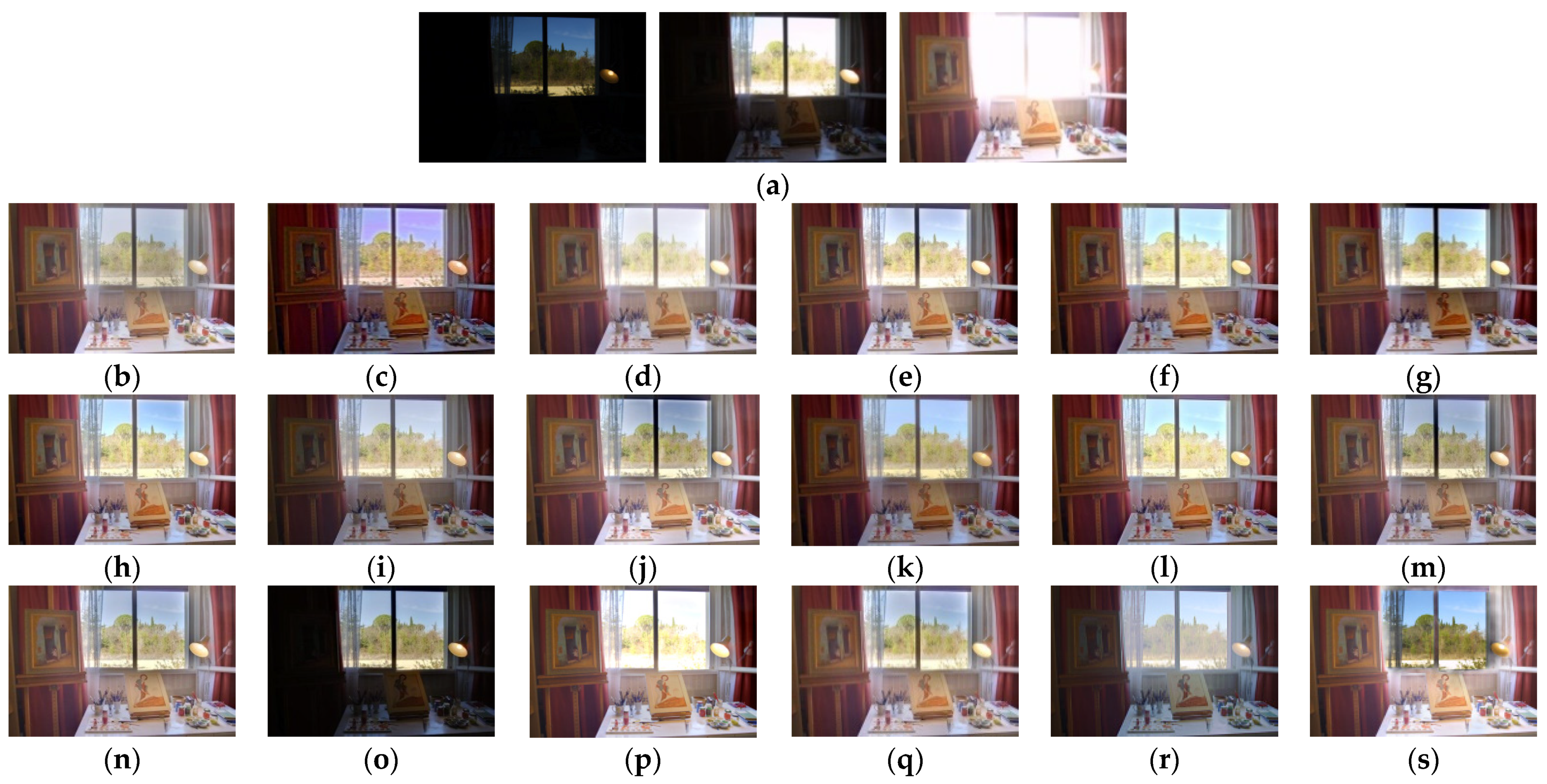
Figure 8 illustrates the fusion results of the “Studio” image sequence from 18 MEF methods. It can be seen that there is a large difference in brightness between the inside and outside of the window. The fused result from the inside of the window given by Yang [50] is still underexposed, and there is a similar problem in Mertens [41], while the overexposed region in the outside of the window from LXN [123] is relatively poorly recovered. Other methods can achieve simultaneous exposure for inside and outside the window. The fusion results of Ma [31], Hayat [115], and IFCNN [82] have color distortion. The results of Liu [114] and Lee [21] are a little blurred. There are halos at the intersections of the sky and the window from the fused results of Wang [48] and LST [42]. LH20 [32] is better than LH21 [33] in color contrast, but the former is worse in detail preservation in the underexposed regions. The fused results of the overexposed and underexposed regions are recovered relatively well from MEFNet [86], while the artifacts and dark region are introduced at the intersection position of these two regions. On the whole, LH20 [32], LH21 [33], Nejati [45], Qi [40], Paul [57], and LZG [46] provide relatively better fusion images in the “Studio” image sequence.
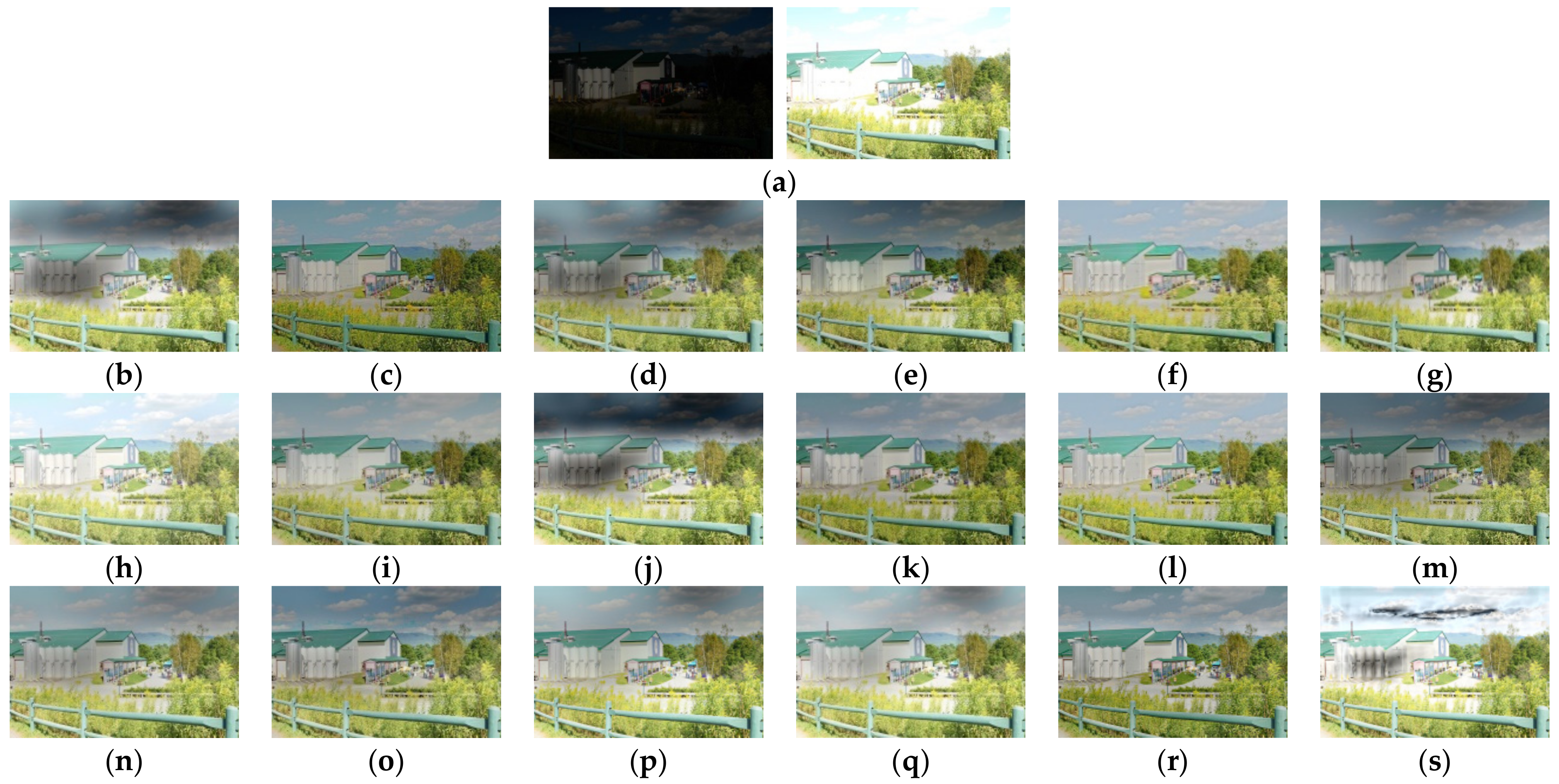
Figure 9 shows the fusion results from the “SICE348” image sequence with a large exposure ratio, and the fused images should preserve the structure and texture details of the sky and architecture. The fusion result from Hayat [115] is a little blurred. The fused image from Qi [40] contains a lot of noise. Yang [50] introduces color distortion. LH21 [33] recovers well in the underexposed region, but the overall color contrast is low. The fused results of Kou [49], Lee [21], Liu [114], LST [42], LXN [123], LZG [46], MEFNet [86], and Wang [48] contain dark regions and the intensity of the fused images distributes non uniformly. IFCNN [81], LH20 [32], Ma [31], Paul [57], Mertens [41], and Nejati [45] perform relatively better on this sequence.
Table 5 lists the average scores of eight metrics from 18 MEF methods on 20 groups of image sequences. The top five performances are displayed in bold for each metric. It can be seen that the spatial domain methods have some advantages in the metrics MI, NIQE, SD, and EN. Ma [31], Qi [40], and LH20 [32] achieve the highest score and also have better subjective performance in most scenes. The transform domain methods have advantages in MEF-SSIM and QAB/F. LST [42] and Nejati [45] achieve the highest score in these two metrics. The two MEF methods based on deep learning may have some problems on the subjective qualitative evaluation in some cases, but they show advantages in multiple metrics. Specifically, IFCNN [81] has some problems in color distortion, but it achieves high scores in MI, PSNR, SD, and AG. In multiple scenes, MEFNet [86] has poor transitions between the edges of the overexposed region and the underexposed region, which result in halo and shadow problems in the fusion images. However, its scores on QAB/F and SD are still high. It can be found that no method can rank in the top five on all eight metrics in test image sequences, which indicates that there is still room for further improvement in studies of the MEF method.
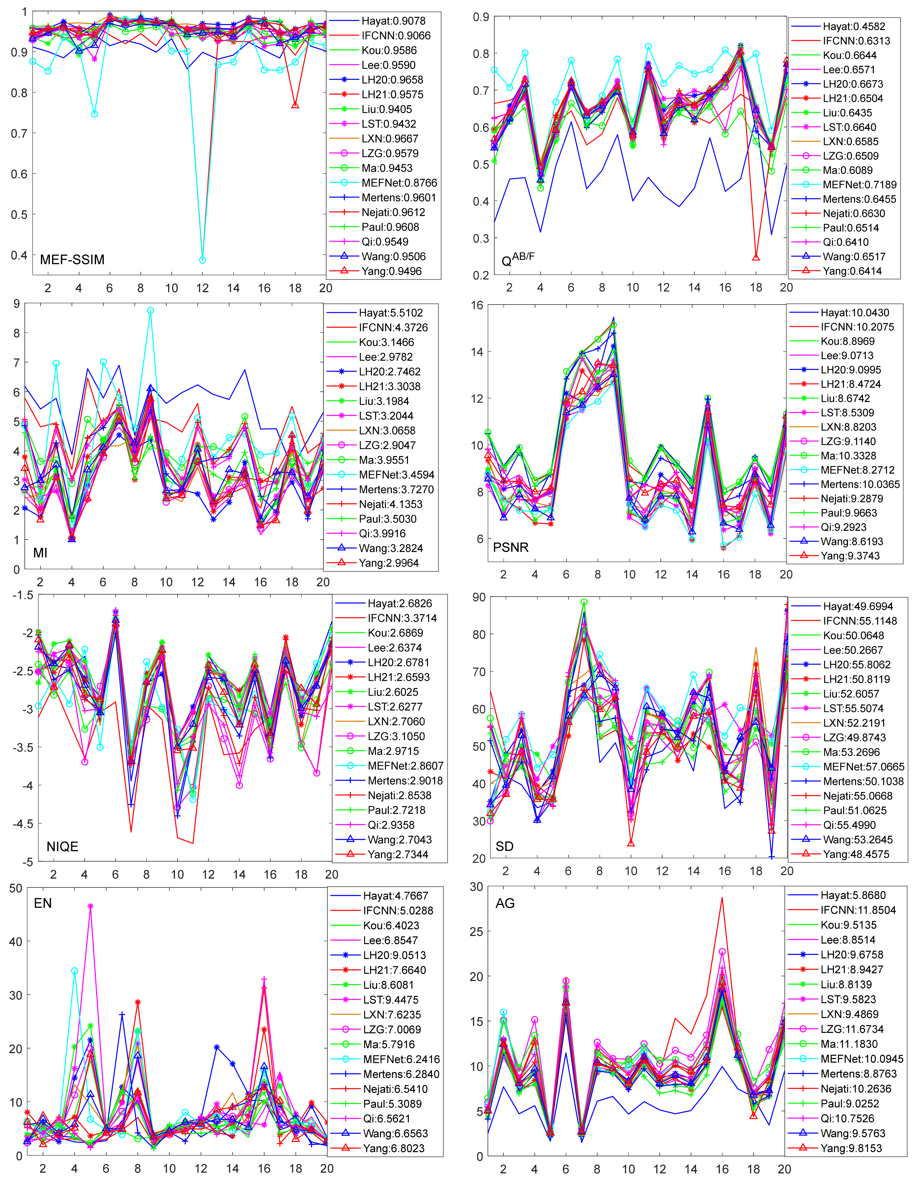
Figure 10 provides more insights on the objective comparison of different MEF methods. Each metric curve can be generated by connecting the scores obtained by a method on 20 image sequences, and the legend gives the average scores. Because there are a total of 18 MEF methods involved, each sub-figure looks a little crowded. Readers can find the eight sub-figures at the following website https://github.com/xfupup/MEF_data (9 January 2022). The curves can be selected in order to zoom in and observe them more clearly. Considering that the lower the NIQE value, the better the performance, we take its negative value (i.e., -NIQE) to illustrate. As can be seen from Figure 10, there is an approximately consistent change trend in the given metrics for the different MEF algorithms. However, different MEF methods may have several changes in each metric. For example, Hayat [115] has a higher score on the MI, but it obtains lower values on other metrics. Additionally, MEFNet [86] has a high score on MEF-SSIM metric, but its score is low on QAB/F.
3.3.2. Testing for Dynamic Scene
This part of the experiment establishes a dataset for the test in a dynamic scene combined with the DeghostingIQASet dataset, including 162 fusion results from six MEF methods on 27 groups of image sequences. The results can be downloaded online at https://github.com/xfupup/MEF_data (9 January 2022). The HDR-VDP-2 scores of 162 fusion results from six methods are listed in Table 6. Figure 11 and Figure 12 illustrate two sets of fusion results from six MEF methods.
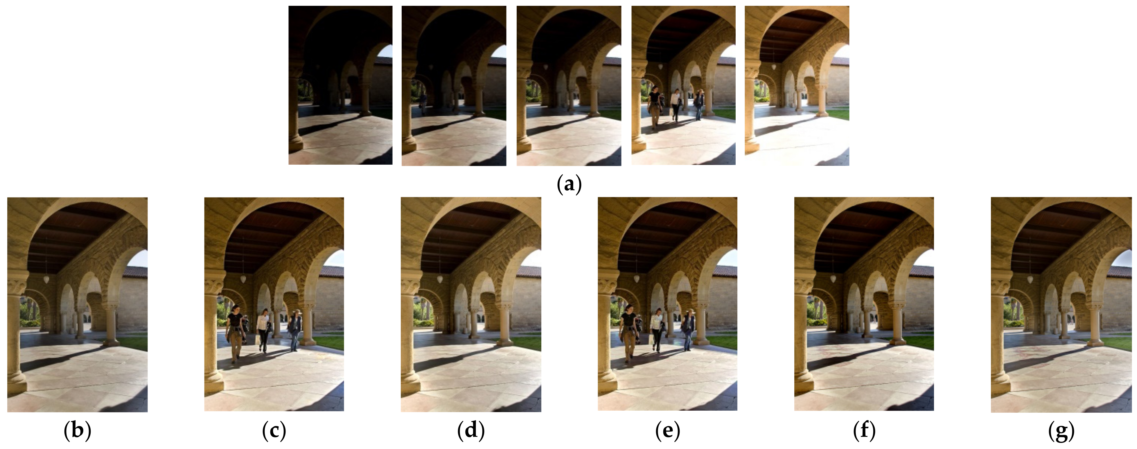
As can be seen in Figure 11, the fusion results will change when different reference images are selected, and all of the methods can remove ghosts in the “Arch” image sequence. Liu [114], Ma [31], Qi [40], and LH21 [33] retain more details in overexposed and underexposed regions, such as sky and ground shadows, while the fused results of Hayat [115] and LH20 [32] are relatively poor. On the roof of buildings, Hayat [115] and LH21 [33] have a good performance in brightness recovery and detail retention. The brightness values of the fusion results from the other four algorithms are low. Overall, the fusion performance of LH21 [33] is the best in vision impression.
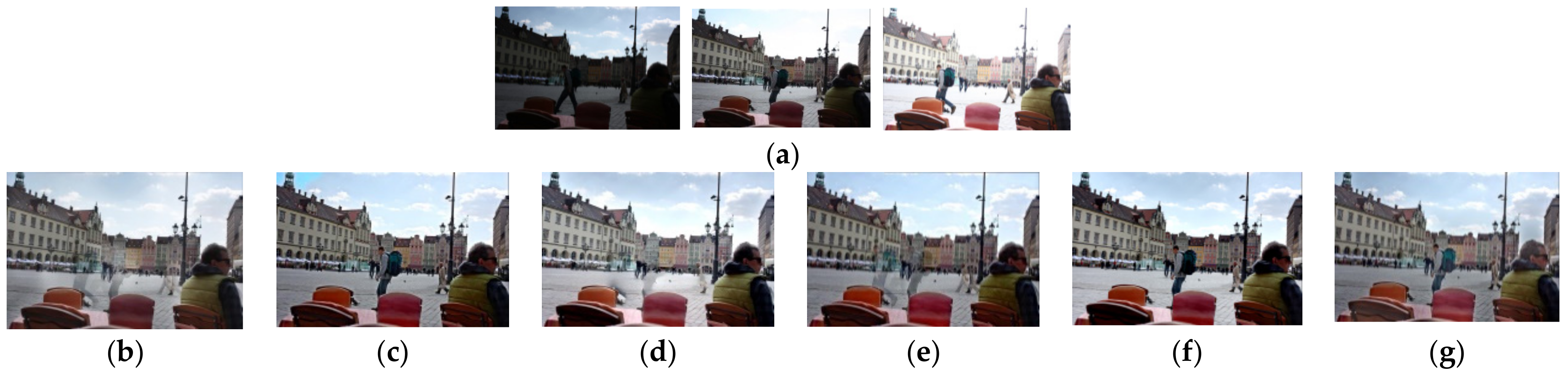
Figure 12 illustrates the fused results on the “Wroclav” image sequence. As can be seen, the fused images obtained by Ma [31], LH20 [32], and LH21 [33] have no ghost artifact. While Liu [114] and Hayat [115] eliminate ghosts, they also produce residual ghosts and broken objects. The ghosts are not entirely removed in Qi [40] and the artifacts still exist. Although Ma [31] and LH20 [32] remove the ghosts, the brightness is relatively dark in the underexposed region. In addition, the brightness of the ground in LH20 [32] is still high, and the color of the sky in Ma [31] is distorted. The fusion performance of LH21 [33] is also the best in this image sequence. The details of the regions that are too bright and too dark in the source images are well preserved in LH21 [33], for example, the hair of the man sitting on the bench.
Table 6 lists the HDR-VDP-2 scores of the different deghosting methods. Black bold font represents the highest score in this image sequence. The underlined font indicates that the subjective evaluation of the fusion result is relatively good, but the HDR-VDP-2 score is excessively low. The underlined bold font means that the subjective assessment is rather bad, but the HDR-VDP-2 score is excessively high. It was found that the selection of reference images has an impact on the score of HDR-VDP-2. When selecting an input image including a moving object consistent with that in the fusion image as the reference image, or selecting an image corresponding to the brightness of the fusion image but inconsistent with the moving object as the reference image, the HDR-VDP-2 scores are quite different. Although Ma [31] scores the highest in multiple image sequences, the details of the underexposed regions of these image sequences were not recovered well. To sum up, the performance of the fusion results from LH21 [33] is best in both subjective evaluation and objective quantitative scores.
3.3.3. Computational Efficiency
This part gives the calculation time of the MEF methods involved in comparison, except the two deep learning-based MEF approaches (these approaches are performed in a parallel calculating way through GPU acceleration and the computational efficiency is very high). All the other 16 methods are implemented in MATLAB 2018a with a 2.50 GHz CPU (Intel(R) Core(TM) i5-7200U) and 16 GB RAM. When fusing two color images with 1000 × 664 pixels in a static scene, Table 7 lists the average running time of these methods.
4. Future Prospects
Although remarkable progress has been made in MEF, there are some issues for future work. This section gives a detailed discussion on development trends based on the review of the existing methods.
- (1)
- Deep learning-based MEF
Although the performance of multi-exposure fusion based on deep learning has been greatly improved, there are still many aspects worthy of further research. i) Establishing a large-scale multi-exposure image dataset is crucial for supervised MEF methods. Some expert photographers may be hired to capture “ground truth”, but it is not an easy task due to the general camera’s limited capture range. In addition, a method similar to Cai [79] may also be adopted. However, the representative methods should be selected from the latest state-of-the-art algorithms. In addition, data augmentation techniques will provide a way to generate a large amount of data without high cost and time requirements [89]. ii) Constructing a practical loss function consisting of several types of metrics and associated with the specific fusion task. Subsequent research should pay more attention to the characteristics of the fusion task itself rather than blindly increasing the scale of the neural networks. The existing methods based on deep learning rarely consider the correlation between MEF and subsequent tasks when constructing the loss function, which often makes the fusion results subjective. Future research may introduce the accuracy of following tasks to guide the fusion process. iii) At present, most of the existing MEF methods based on deep learning are only suitable for static scenes. In addition, there are also few multi-exposure images in dynamic scenes, so it is necessary to capture and collect multi-exposure images in dynamic scenes.
- (2)
- MEF in dynamic scene
Most off-the-shelf MEF methods focus on solving the fusion of the images with different exposure levels in a static scene. However, the source images are often misaligned due to camera jitter and moving objects in the application. The fusion images will suffer from ghosts, image blurring, halo artifacts, and other problems. Although some deghosting MEF methods have been proposed in recent years, they cannot solve these issues robustly. A way to address camera jitter is to use registration, but the preprocessing dependent on the registration algorithm may lead to some limitations, such as low efficiency and dependence on the registration accuracy. Therefore, it is necessary to develop a non-registered method to implicitly realize MEF. Regarding moving objects, selecting the appropriate reference image is also worthy of attention.
- (3)
- The higher-quality MEF evaluation metrics
From the discussions from Section 3, it can be found that there may be inconsistency between qualitative and quantitative evaluations of the fused results. Some methods that show good qualitative performance may not perform well in quantitative comparison and vice versa. For example, one of the most commonly used evaluation metrics, MEF-SSIM, still cannot precisely describe the fused images’ subjective quality. Several methods also show different performances on different types of metrics. This brings difficulties to the comprehensive evaluation of the MEF methods. Therefore, it is necessary to explore more accurate evaluation metrics from the perspective of the human visual system in future research. In addition, there are few studies on developing appropriate evaluation metrics for MEF in dynamic scenes. These are issues that need attention in the future.
- (4)
- Task-oriented MEF
There are few MEF works developed for specific tasks in industry, remote sensing, and other fields. Most research aims at natural images to verify the effectiveness of the proposed methods, and no algorithms can be universal to all scenes. Therefore, it is important to develop and fine-tune suitable MEF algorithms for more specific tasks.
- (5)
- Real-time MEF
From the perspective of application requirements, the MEF technique is the preprocessing of many visual tasks, such as video surveillance, target recognition, target tracking, and other applications. The performance of the MEF methods directly affects the accuracy of the whole research. Some applications have high requirements for the computational efficiency of the algorithm. However, the operating efficiency of the current MEF methods is low owing to the complex transformation, function decomposition, and iterative optimization, which limits the applications of the MEF algorithms in some real-time tasks. Therefore, the development of real-time MEF algorithms is essential, which will cause MEF to have more expensive application areas.
Therefore, based on the above review and prospects, we have not reached the upper limit of MEF, and it remains a long-term task to study higher-quality MEF algorithms and evaluation metrics.
5. Conclusions
MEF is an essential technique for integrating image information with different exposure levels, which can more comprehensively understand the scene. To follow the latest development in this field, this paper summarizes the existing MEF methods and presents a literature review. These MEF methods can generally be divided into spatial domain, transform domain, and deep learning. In addition, ghost removal MEF methods are also discussed as a supplement. According to the core idea, each class is investigated and further divided into several sub-categories. We analyze the representative methods in each sub-category and provide some systematic summaries. A detailed comparative study for the current MEF algorithms in static and dynamic scenes is carried out. The experiment performs subjective and objective evaluations of the 18 MEF approaches using nine commonly used objective fusion metrics. We have released the relevant resources online for comparison, including input image sequences, fusion results, and curves. There are still many challenges in MEF techniques and objective fusion performance evaluation due to the limitations of sensor noise, camera jitter, moving objects, and computational complexity. Finally, some prospects and potential research directions are proposed based on our observations. We expect that the organized overview of MEF methods can help relevant researchers to better understand the current development of MEF methods.
Author Contributions
F.X. provided the idea. F.X. and J.L. designed the experiments. Y.S. and X.W. analyzed the experiments. F.X. and H.S. wrote the paper. All authors have read and agreed to the published version of the manuscript.
Funding
This research was funded by the National Natural Science Foundation of China grant number No.62175233.
Institutional Review Board Statement
Not applicable.
Informed Consent Statement
Not applicable.
Data Availability Statement
The data presented in this study are available in the article.
Acknowledgments
The authors wish to thank the associate editor and reviewers for their valuable suggestions.
Conflicts of Interest
The authors declare no conflict of interest.
References
- Huang, L.; Li, Z.; Xu, C.; Feng, B. Multi-exposure image fusion based on feature evaluation with adaptive factor. IET Image Process. 2021, 15, 3211–3220. [Google Scholar] [CrossRef]
- Shen, R.; Cheng, I.; Basu, A. QoE-based multi-exposure fusion in hierarchical multivariate gaussian CRF. IEEE Trans. Image Process. 2013, 22, 2469–2478. [Google Scholar] [CrossRef]
- Aggarwal, M.; Ahuja, N. Split aperture imaging for high dynamic range. In Proceedings of the 8th IEEE International Conference on Computer Vision(ICCV), Vancouver, BC, Canada, 7–14 July 2001; pp. 10–16. [Google Scholar]
- Tumblin, J.; Agrawal, A.; Raskar, R. Why I want a gradient camera. In Proceedings of the IEEE Computer Society Conference on Computer Vision and Pattern Recognition(CVPR), San Diego, CA, USA, 20–25 June 2005; pp. 103–110. [Google Scholar]
- Li, S.; Kang, X.; Fang, L.; Hu, J.; Yin, H. Pixel-level image fusion: A survey of the state of the art. Inf. Fusion 2017, 33, 100–112. [Google Scholar] [CrossRef]
- Nie, T.; Huang, L.; Liu, H.; Xiansheng Li, X. Multi-exposure fusion of gray images under low illumination based on low-rank decomposition. Remote Sens. 2021, 13, 204. [Google Scholar] [CrossRef]
- Kim, J.; Ryu, J.; Kim, J. Deep gradual flash fusion for low-light enhancement. J. Vis. Commun. Image Represent. 2020, 72, 102903. [Google Scholar] [CrossRef]
- Galdran, A. Image dehazing by artificial multiple-exposure image fusion. Signal Process. 2018, 149, 135–147. [Google Scholar] [CrossRef]
- Wang, X.; Sun, Z.; Zhang, Q.; Fang, Y. Multi-exposure decomposition-fusion model for high dynamic range image saliency detection. IEEE Trans. Circuits Syst. Video Technol. 2020, 30, 4409–4420. [Google Scholar] [CrossRef]
- Zhang, X. Benchmarking and comparing multi-exposure image fusion algorithms. Inf. Fusion 2021, 74, 111–131. [Google Scholar] [CrossRef]
- Burt, P.; Kolczynski, R. Enhanced image capture through fusion. In Proceedings of the International Conference on Computer Vision (ICCV), Berlin, Germany, 11–14 May 1993; pp. 173–182. [Google Scholar]
- Bertalmío, M.; Levine, S. Variational approach for the fusion of exposure bracketed pairs. IEEE Trans. Image Process. 2013, 22, 712–723. [Google Scholar] [CrossRef]
- Yang, Y.; Wu, S.; Wang, X.; Li, Z. Exposure interpolation for two large-exposure-ratio images. IEEE Access 2020, 8, 227141–227151. [Google Scholar] [CrossRef]
- Prabhakar, K.R.; Agrawal, S.; Babu, R.V. Self-gated memory recurrent network for efficient scalable HDR deghosting. IEEE Trans. Comput. Imaging 2021, 7, 1228–1239. [Google Scholar]
- Liu, Y.; Wang, L.; Cheng, J.; Chang, L.; Xun, C. Multi-focus image fusion: A Survey of the state of the art. Inf. Fusion 2020, 64, 71–91. [Google Scholar] [CrossRef]
- Chen, Y.; Jiang, G.; Yu, M.; Yang, Y.; Ho, Y.S. Learning stereo high dynamic range imaging from a pair of cameras with different exposure parameters. IEEE Trans. Comput. Imaging 2020, 6, 1044–1058. [Google Scholar] [CrossRef]
- Xu, H.; Ma, J.; Zhang, X. MEF-GAN: Multi-exposure image fusion via generative adversarial networks. IEEE Trans. Image Process. 2020, 29, 7203–7216. [Google Scholar] [CrossRef]
- Chang, M.; Feng, H.; Xu, Z.; Li, Q. Robust ghost-free multiexposure fusion for dynamic scenes. J. Electron. Imaging 2018, 27, 033023. [Google Scholar] [CrossRef]
- Karaduzovic-Hadziabdic, K.; Telalovic, J.H.; Mantiuk, R.K. Assessment of multi-exposure HDR image deghosting methods. Comput. Graph. 2017, 63, 1–17. [Google Scholar] [CrossRef] [Green Version]
- Bruce, N.D.B. Expoblend: Information preserving exposure blending based on normalized log-domain entropy. Comput. Graph. 2014, 39, 12–23. [Google Scholar] [CrossRef]
- Lee, L.-H.; Park, J.S.; Cho, N.I. A multi-exposure image fusion based on the adaptive weights reflecting the relative pixel intensity and global gradient. In Proceedings of the 25th IEEE International Conference on Image Processing (ICIP), Athens, Greece, 7–10 October 2018; pp. 1737–1741. [Google Scholar]
- Kinoshita, Y.; Kiya, H. Scene segmentation-based luminance adjustment for multi-exposure image fusion. IEEE Trans. Image Process. 2019, 28, 4101–4115. [Google Scholar] [CrossRef] [Green Version]
- Xu, Y.; Sun, B. Color-compensated multi-scale exposure fusion based on physical features. Optik 2020, 223, 165494. [Google Scholar] [CrossRef]
- Ulucan, O.; Karakaya, D.; Turkan, M. Multi-exposure image fusion based on linear embeddings and watershed masking. Signal Process. 2021, 178, 107791. [Google Scholar] [CrossRef]
- Raman, S.; Chaudhuri, S. Bilateral Filter Based Compositing for Variable Exposure Photography. The Eurographics Association: Geneve, Switzerland, 2009; pp. 1–4. [Google Scholar]
- Li, S.; Kang, X. Fast multi-exposure image fusion with median filter and recursive filter. IEEE Trans. Consum. Electron. 2012, 58, 626–632. [Google Scholar] [CrossRef] [Green Version]
- Wang, C.; He, C.; Xu, M. Fast exposure fusion of detail enhancement for brightest and darkest regions. Vis. Comput. 2021, 37, 1233–1243. [Google Scholar] [CrossRef]
- Goshtasby, A.A. Fusion of multi-exposure images. Image Vis. Comput. 2005, 23, 611–618. [Google Scholar] [CrossRef]
- Huang, F.; Zhou, D.; Nie, R. A Color Multi-exposure image fusion approach using structural patch decomposition. IEEE Access 2018, 6, 42877–42885. [Google Scholar] [CrossRef]
- Ma, K.; Wang, Z. Multi-exposure image fusion: A patch-wise approach. In Proceedings of the 2015 IEEE International Conference on Image Processing, Quebec City, QC, Canada, 27–30 September 2015; pp. 1717–1721. [Google Scholar]
- Ma, K.; Li, H.; Yong, H.; Wang, Z.; Meng, D.; Zhang, L. Robust multi-exposure image fusion: A structural patch decomposition approach. IEEE Trans. Image Process. 2017, 26, 2519–2532. [Google Scholar] [CrossRef]
- Li, H.; Ma, K.; Yong, H.; Zhang, L. Fast multi-scale structural patch decomposition for multi-exposure image fusion. IEEE Trans. Image Process. 2020, 29, 5805–5816. [Google Scholar] [CrossRef]
- Li, H.; Chan, T.N.; Qi, X.; Xie, W. Detail-preserving multi-exposure fusion with edge-preserving structural patch decomposition. IEEE Trans. Circuits Syst. Video Technol. 2021, 31, 1–12. [Google Scholar] [CrossRef]
- Wang, S.; Zhao, Y. A novel patch-based multi-exposure image fusion using super-pixel segmentation. IEEE Access 2020, 8, 39034–39045. [Google Scholar] [CrossRef]
- Shen, R.; Cheng, I.; Shi, J.; Basu, A. Generalized random walks for fusion of multi-exposure images. IEEE Trans. Image Process. 2011, 20, 3634–3646. [Google Scholar] [CrossRef]
- Li, Z.; Zheng, J.; Rahardja, S. Detail-enhanced exposure fusion. IEEE Trans. Image Process. 2012, 21, 4672–4676. [Google Scholar]
- Song, M.; Tao, D.; Chen, C. Probabilistic exposure fusion. IEEE Trans. Image Process. 2012, 21, 341–357. [Google Scholar] [CrossRef] [PubMed]
- Liu, S.; Zhang, Y. Detail-preserving underexposed image enhancement via optimal weighted multi-exposure fusion. IEEE Trans. Consum. Electron. 2019, 65, 303–311. [Google Scholar] [CrossRef]
- Ma, K.; Duanmu, Z.; Yeganeh, H.; Wang, Z. Multi-exposure image fusion by optimizing a structural similarity index. IEEE Trans. Comput. Imaging 2018, 4, 60–72. [Google Scholar] [CrossRef]
- Qi, G.; Chang, L.; Luo, Y.; Chen, Y. A precise multi-exposure image fusion method based on low-level features. Sensors 2020, 20, 1597. [Google Scholar] [CrossRef] [Green Version]
- Mertens, T.; Kautz, J.; Reeth, F.V. Exposure fusion. In Proceedings of the 15th Pacific Conference on Computer Graphics and Applications, Maui, HI, USA, 4 December 2007; pp. 382–390. [Google Scholar]
- Li, S.; Kang, X.; Hu, J. Image fusion with guided filtering. IEEE Trans. Image Process. 2013, 22, 2864–2875. [Google Scholar] [PubMed]
- Shen, J.; Zhao, Y.; Yan, S.; Li, X. Exposure fusion using boosting laplacian pyramid. IEEE Trans. Cybern. 2014, 44, 1579–1590. [Google Scholar] [CrossRef]
- Singh, H.; Kumar, V.; Bhooshan, S. A novel approach for detail-enhanced exposure fusion using guided filter. Sci. World J. 2014, 2014, 659217. [Google Scholar] [CrossRef]
- Nejati, M.; Karimi, M.; Soroushmehr, S.M.R.; Karimi, N.; Samavi, S.; Najarian, K. Fast exposure fusion using exposuredness function. In Proceedings of the IEEE International Conference on Image Processing (ICIP), Beijing, China, 17–20 September 2017; pp. 2234–2238. [Google Scholar]
- Li, Z.; Wen, C.; Zheng, J. Detail-enhanced multi-scale exposure fusion. IEEE Trans. Image Process. 2017, 26, 1243–1252. [Google Scholar] [CrossRef]
- Yan, Q.; Zhu, Y.; Zhou, Y.; Sun, J.; Zhang, L.; Zhang, Y. Enhancing image visuality by multi-exposure fusion. Pattern Recognit. Lett. 2019, 127, 66–75. [Google Scholar] [CrossRef]
- Wang, Q.; Chen, W.; Wu, X.; Li, Z. Detail-enhanced multi-scale exposure fusion in YUV color space. IEEE Trans. Circuits Syst. Video Technol. 2019, 26, 1243–1252. [Google Scholar] [CrossRef]
- Kou, F.; Li, Z.; Wen, C.; Chen, W. Edge-preserving smoothing pyramid based multi-scale exposure fusion. J. Vis. Commun. Image Represent. 2018, 53, 235–244. [Google Scholar] [CrossRef]
- Yang, Y.; Cao, W.; Wu, S.; Li, Z. Multi-scale fusion of two large-exposure-ratio image. IEEE Signal Process. Lett. 2018, 25, 1885–1889. [Google Scholar] [CrossRef]
- Qu, Z.; Huang, X.; Chen, K. Algorithm of multi-exposure image fusion with detail enhancement and ghosting removal. J. Electron. Imaging 2019, 28, 013022. [Google Scholar] [CrossRef]
- Lin, Y.-H.; Hua, K.-L.; Lu, H.-H.; Sun, W.-L.; Chen, Y.-Y. An adaptive exposure fusion method using fuzzy logic and multivariate normal conditional random fields. Sensors 2019, 19, 1–23. [Google Scholar] [CrossRef] [Green Version]
- Gu, B.; Li, W.; Wong, J.; Zhu, M.; Wang, M. Gradient field multi-exposure images fusion for high dynamic range image visualization. J. Vis. Commun. Image Represent. 2012, 23, 604–610. [Google Scholar] [CrossRef]
- Zhang, W.; Cham, W.-K. Gradient-directed multiexposure composition. IEEE Trans. Image Process. 2012, 21, 2318–2323. [Google Scholar] [CrossRef]
- Wang, C.; Yang, Q.; Tang, X.; Ye, Z. Salience preserving image fusion with dynamic range compression. In Proceedings of the IEEE International Conference on Image Processing, Atlanta, GA, USA, 8–11 October 2006; pp. 989–992. [Google Scholar]
- Hara, K.; Inoue, K.; Urahama, K. A differentiable approximation approach to contrast aware image fusion. IEEE Signal Process. Lett. 2014, 21, 742–745. [Google Scholar] [CrossRef]
- Paul, S.; Sevcenco, J.S.; Agathoklis, P. Multi-exposure and multi-focus image fusion in gradient domain. J. Circuits Syst. Comput. 2016, 25, 1650123. [Google Scholar] [CrossRef] [Green Version]
- Liu, Y.; Zhou, D.; Nie, R.; Hou, R.; Ding, Z. Construction of high dynamic range image based on gradient information transformation. IET Image Process. 2020, 14, 1327–1338. [Google Scholar] [CrossRef]
- Wang, X.; Shen, S.; Ning, C.; Huang, F.; Gao, H. Multiclass remote sensing object recognition based on discriminative sparse representation. Appl. Opt. 2016, 55, 1381–1394. [Google Scholar] [CrossRef]
- Wang, J.; Liu, H.; He, N. Exposure fusion based on sparse representation using approximate K-SVD. Neurocomputing 2014, 135, 145–154. [Google Scholar] [CrossRef]
- Shao, H.; Jiang, G.; Yu, M.; Song, Y.; Jiang, H.; Peng, Z.; Chen, F. Halo-free multi-exposure image fusion based on sparse representation of gradient features. Appl. Sci. 2018, 8, 1543. [Google Scholar] [CrossRef] [Green Version]
- Yang, Y.; Wu, J.; Huang, S.; Lin, P. Multi-exposure estimation and fusion based on a sparsity exposure dictionary. IEEE Trans. Instrum. Meas. 2020, 69, 4753–4767. [Google Scholar] [CrossRef]
- Lee, G.-Y.; Lee, S.-H.; Kwon, H.-J. DCT-based HDR exposure fusion using multiexposed image sensors. J. Sensors 2017, 2017, 1–14. [Google Scholar] [CrossRef]
- Martorell, O.; Sbert, C.; Buades, A. Ghosting-free DCT based multi-exposure image fusion. Signal Process. Image Commun. 2019, 78, 409–425. [Google Scholar] [CrossRef]
- Zhang, W.; Liu, X.; Wang, W.; Zeng, Y. Multi-exposure image fusion based on wavelet transform. Int. J. Adv. Robot. Syst. 2018, 15, 1–19. [Google Scholar] [CrossRef] [Green Version]
- Zhang, Y.; Liu, T.; Singh, M.; Cetintas, E.; Luo, Y.; Rivenson, Y.; Larin, K.V.; Ozcan, A. Neural network-based image reconstruction in swept-source optical coherence tomography using undersampled spectral data. Light. Sci. Appl. 2021, 10, 390–400. [Google Scholar] [CrossRef]
- Li, X.; Zhang, G.; Qiao, H.; Bao, F.; Deng, Y.; Wu, J.; He, Y.; Yun, J.; Lin, X.; Xie, H.; et al. Unsupervised content-preserving transformation for optical microscopy. Light. Sci. Appl. 2021, 10, 1658–1671. [Google Scholar] [CrossRef]
- Wu, S.; Xu, J.; Tai, Y.W. Deep high dynamic range imaging with large foreground motions. In Proceedings of the European Conference on Computer Vision, Munich, Germany, 9 October 2018; pp. 120–135. [Google Scholar]
- Yan, Q.; Gong, D.; Zhang, P. Multi-scale dense networks for deep high dynamic range imaging. In Proceedings of the 2019 IEEE Winter Conference on Applications of Computer Vision (WACV), Waikoloa, HI, USA, 7–11 January 2019; pp. 41–50. [Google Scholar]
- Yan, Q.; Gong, D.; Shi, Q. Attention guided network for ghost-free high dynamic range imaging. In Proceedings of the 2019 IEEE/CVF Conference on Computer Vision and Pattern Recognition (CVPR), Long Beach, CA, USA, 15–20 June 2019; pp. 1751–1760. [Google Scholar]
- Wang, J.; Li, X.; Liu, H. Exposure fusion using a relative generative adversarial network. IEICE Trans. Inf. Syst. 2021, E104D, 1017–1027. [Google Scholar] [CrossRef]
- Vu, T.; Nguyen, C.V.; Pham, T.X.; Luu, T.M.; Yoo, C.D. Fast and efficient image quality enhancement via desubpixel convolutional neural networks. In Proceedings of the European Conference on Computer Vision, Munich, Germany, 23 January 2019; pp. 243–259. [Google Scholar]
- Jeon, M.; Jeong, Y.S. Compact and accurate scene text detector. Appl. Sci. 2020, 10, 2096. [Google Scholar] [CrossRef] [Green Version]
- Kalantari, N.K.; Ramamoorthi, R. Deep high dynamic range imaging of dynamic scenes. ACM Trans. Graph. 2017, 36, 144. [Google Scholar] [CrossRef]
- Wang, J.; Wang, W.; Xu, G.; Liu, H. End-to-end exposure fusion using convolutional neural network. IEICE Trans. Inf. Syst. 2018, 101, 560–563. [Google Scholar] [CrossRef] [Green Version]
- Deng, J.; Dong, W.; Socher, R.; Li, L.J.; Li, K.; Li, F.F. Imagenet: A large-scale hierarchical image database. In Proceedings of the IEEE Conference on Computer Vision and Pattern Recognition(CVPR), Miami, FL, USA, 20–25 June 2009; pp. 248–255. [Google Scholar]
- Li, H.; Zhang, L. Multi-exposure fusion with CNN features. In Proceedings of the 25th IEEE International Conference on Image Processing (ICIP), Athens, Greece, 7–10 October 2018; pp. 1723–1727. [Google Scholar]
- Lahoud, F.; Süsstrunk, S. Fast and efficient zero-learning image fusion. arXiv 2019, arXiv:1902.00730. [Google Scholar]
- Cai, J.; Gu, S.; Zhang, L. Learning a deep single image contrast enhancer from multi-exposure images. IEEE Trans. Image Process. 2018, 27, 2049–2062. [Google Scholar] [CrossRef]
- Liu, Q.; Leung, H. Variable augmented neural network for decolorization and multi-exposure fusion. Inf. Fusion 2019, 46, 114–127. [Google Scholar] [CrossRef]
- Chen, Y.; Yu, M.; Jiang, G.; Peng, Z.; Chen, F. End-to-end single image enhancement based on a dual network cascade model. J. Vis. Commun. Image Represent. 2019, 61, 284–295. [Google Scholar] [CrossRef]
- Zhang, Y.; Liu, Y.; Sun, P.; Yan, H.; Zhao, X.; Zhang, L. IFCNN: A general image fusion framework based on convolutional neural network. Inf. Fusion 2020, 54, 99–118. [Google Scholar] [CrossRef]
- Fang, A.; Zhao, X.; Yang, J.; Qin, B.; Zhang, Y. A light-weight, efficient, and general cross-modal image fusion network. Neurocomputing 2021, 463, 198–211. [Google Scholar] [CrossRef]
- Prabhakar, K.P.; Srikar, V.S.; Babu, R.V. Deepfuse: A deep unsupervised approach for exposure fusion with extreme exposure image pairs. In Proceedings of the IEEE International Conference on Computer Vision (ICCV), Venice, Italy, 22–29 October 2017; pp. 4724–4732. [Google Scholar]
- Ma, K.; Zeng, K.; Wang, Z. Perceptual quality assessment for multi-exposure image fusion. IEEE Trans. Image Process. 2015, 24, 3345–3356. [Google Scholar] [CrossRef]
- Ma, K.; Duanmu, Z.; Zhu, H.; Fang, Y.; Wang, Z. Deep guided learning for fast multi-exposure image fusion. IEEE Trans. Image Process. 2020, 29, 2808–2819. [Google Scholar] [CrossRef]
- Qi, Y.; Zhou, S.; Zhang, Z.; Luo, S.; Lin, X.; Wang, L.; Qiang, B. Deep unsupervised learning based on color un-referenced loss functions for multi-exposure image fusion. Inf. Fusion 2021, 66, 18–39. [Google Scholar] [CrossRef]
- Xu, H.; Ma, J.; Jiang, J.; Guo, X.; Ling, H. U2Fusion: A unified unsupervised image fusion network. IEEE Trans. Pattern Anal. Mach. Intell. 2020, 44, 502–518. [Google Scholar] [CrossRef] [PubMed]
- Gao, M.; Wang, J.; Chen, Y.; Du, C. An improved multi-exposure image fusion method for intelligent transportation system. Electronics 2021, 10, 383. [Google Scholar] [CrossRef]
- Chen, S.Y.; Chuang, Y.Y. Deep exposure fusion with deghosting via homography estimation and attention learning. In Proceedings of the IEEE International Conference on Acoustics, Speech and Signal Processing (ICASSP), Barcelona, Spain, 4–8 May 2020; pp. 1464–1468. [Google Scholar]
- Yang, Z.; Chen, Y.; Le, Z.; Ma, Y. GANFuse: A novel multi-exposure image fusion method based on generative adversarial networks. Neural Comput. Appl. 2021, 33, 6133–6145. [Google Scholar] [CrossRef]
- Tursun, O.T.; Akyüz, A.O.; Erdem, A.; Erdem, E. The state of the art in HDR deghosting: A survey and evaluation. Comput. Graphics 2015, 34, 683–707. [Google Scholar] [CrossRef]
- Yan, Q.; Gong, D.; Shi, J.Q.; Hengel, A.; Sun, J.; Zhu, Y.; Zhang, Y. High dynamic range imaging via gradient-aware context aggregation network. Pattern Recogn. 2022, 122, 108342. [Google Scholar] [CrossRef]
- Woo, S.M.; Ryu, J.H.; Kim, J.O. Ghost-free deep high-dynamic-range imaging using focus pixels for complex motion scenes. IEEE Trans. Image Process. 2021, 30, 5001–5016. [Google Scholar] [CrossRef] [PubMed]
- Cerman, L.; Hlaváč, V. Exposure time estimation for high dynamic range imaging with hand held camera. In Proceedings of the Computer Vision Winter Workshop, Telc, Czech Republic, 6–8 February 2006; pp. 1–6. [Google Scholar]
- Gevrekci, M.; Gunturk, K.B. On geometric and photometric registration of images. In Proceedings of the 2007 IEEE International Conference on Acoustics, Speech and Signal Processing, Honolulu, HI, USA, 15–20 April 2007; pp. 1261–1264. [Google Scholar]
- Yao, S. Robust image registration for multiple exposure high dynamic range image synthesis. In Proceedings of the SPIE, Conference on Image Processing: Algorithms and Systems IX, San Francisco, CA, USA, 24–25 January 2011. [Google Scholar]
- Im, J.; Lee, S.; Paik, J. Improved elastic registration for ghost artifact free high dynamic range imaging. IEEE Trans. Consum. Electron. 2011, 57, 932–935. [Google Scholar] [CrossRef]
- Khan, E.A.; Akyuz, A.O.; Reinhard, E. Ghost removal in high dynamic range images. In Proceedings of the IEEE International Conference on Image Processing, Atlanta, GA, USA, 8–11 October 2006; pp. 2005–2008. [Google Scholar]
- Pedone, M.; Heikkil, J. Constrain propagation for ghost removal in high dynamic range images. VISAPP 2008. In Proceedings of the 3rd International Conference on Computer Vision Theory and Applications, Funchal, Madeira, Portugal, 22–25 January 2008; pp. 36–41. [Google Scholar]
- Zhang, W.; Cham, W.K. Gradient-directed composition of multi-exposure images. In Proceedings of the IEEE Conference on Computer Vision and Pattern Recognition (CVPR), San Francisco, CA, USA, 13–18 June 2010; pp. 530–536. [Google Scholar]
- Wang, Z.; Liu, Q.; Ikenaga, T. Robust ghost-free high-dynamic-range imaging by visual salience based bilateral motion detection and stack extension based exposure fusion. IEICE Trans. Fundam. Electron. Commun. Computer Sci. 2017, E100, 2266–2274. [Google Scholar] [CrossRef]
- Li, Z.; Zheng, J.; Zhu, Z.; Wu, S. Selectively detail-enhanced fusion of differently exposed images with moving objects. IEEE Trans. Image Process. 2014, 23, 4372–4382. [Google Scholar] [CrossRef]
- Jacobs, K.; Loscos, C.; Ward, G. Automatic high-dynamic range image generation for dynamic scenes. IEEE Comput. Graph. Appl. 2008, 28, 84–93. [Google Scholar] [CrossRef] [PubMed]
- Pece, F.; Kautz, J. Bitmap movement detection: HDR for dynamic scenes. In Proceedings of the IEEE Conference on Visual Media Production, London, UK, 17–18 November 2010; pp. 1–8. [Google Scholar]
- Silk, S.; Lang, J. Fast high dynamic range image deghosting for arbitrary scene motion. In Proceedings of the Graphics Interface, Toronto, ON, Canada, 28–30 May 2012; pp. 85–92. [Google Scholar]
- Zhang, W.; Cham, W.K. Reference-guided exposure fusion in dynamic scenes. J. Vis. Commun. Image Represent. 2012, 23, 467–475. [Google Scholar] [CrossRef]
- Granados, M.; Tompkin, J.; Kim, K.I.; Theobalt, C. Automatic noise modeling for ghost-free HDR reconstruction. ACM Trans. Graph. 2013, 32, 201. [Google Scholar] [CrossRef]
- Lee, C.; Li, Y.; Monga, V. Ghost-free high dynamic range imaging via rank minimization. IEEE Signal Process. Lett. 2014, 21, 1045–1049. [Google Scholar]
- Wang, C.; He, C. A novel deghosting method for exposure fusion. Multimed. Tools Appl. 2018, 77, 31911–31928. [Google Scholar] [CrossRef]
- Zimmer, H.; Bruhn, A.; Weickert, J. Freehand HDR Imaging of Moving Scenes with Simultaneous Resolution Enhancement. Comput. Graph. 2011, 30, 405–414. [Google Scholar] [CrossRef]
- Jinno, T.; Okuda, M. Multiple exposure fusion for high dynamic range image acquisition. IEEE Trans. Image Process. 2012, 21, 358–365. [Google Scholar] [CrossRef]
- Ferradans, S.; Bertalmío, M.; Provenzi, E.; Caselles, V. Generation of HDR images in non-static conditions based on gradient fusion. In Proceedings of the 3rd International Conference on Computer Vision Theory and Applications, Barcelona, Spain, 11 September 2012; pp. 31–37. [Google Scholar]
- Liu, Y.; Wang, Z. Dense SIFT for ghost-free multi-exposure fusion. J. Vis. Commun. Image Represent. 2015, 31, 208–224. [Google Scholar] [CrossRef]
- Hayat, N.; Imran, M. Ghost-free multi exposure image fusion technique using dense sift descriptor and guided filter. J. Vis. Commun. Image Represent. 2019, 62, 295–308. [Google Scholar] [CrossRef]
- Zhang, W.; Hu, S.; Liu, K.; Yao, J. Motion-free exposure fusion based on inter-consistency and intra-consistency. Inf. Sci. 2017, 376, 190–201. [Google Scholar] [CrossRef]
- Sen, P.; Kalantari, N.K.; Yaesoubi, M.; Darabi, S. Robust patch-based HDR reconstruction of dynamic scenes. ACM Trans. Graph. 2012, 31, 203. [Google Scholar] [CrossRef]
- Hu, J.; Gallo, Q.; Pulli, K. Exposure stacks of live scenes with hand-held cameras. In Proceedings of the European Conference on Computer Vision (ECCV), Firenze, Italy, 7–13 October 2012; pp. 499–512. [Google Scholar]
- Hu, J.; Gallo, O.; Pulli, K.; Sun, X. HDR deghosting: How to deal with saturation? In Proceedings of the 2013 IEEE Conference on Computer Vision and Pattern Recognition, Portland, OR, USA, 23–28 June 2013; pp. 1163–1170. [Google Scholar]
- Tursun, O.T.; Akyüz, A.O.; Erdem, A.; Erdem, E. Evaluating deghosting algorithms for HDR images. In Proceedings of the Signal Processing and Communications Applications Conference (SIU), Trabzon, Turkey, 23–25 April 2014; pp. 1275–1278. [Google Scholar]
- Nosko, S.; Musil, M.; Zemcik, P.; Juranek, R. Color HDR video processing architecture for smart camera. J. Real-Time Image Pr. 2020, 17, 555–566. [Google Scholar] [CrossRef]
- Castro, T.K.; Chapiro, A.; Cicconet, M.; Velho, L. Towards mobile HDR video. In Proceedings of the Eurographics Areas Papers, Llandudno, UK, 11–15 April 2011; pp. 75–76. [Google Scholar]
- Liu, X.; Liu, Y.; Zhu, C. Perceptual multi-exposure image fusion. IEEE Trans. Multimed. 2022. submitted for publication. [Google Scholar]
- Tursun, O.; Akyüz, A.; Erdem, A.; Erdem, E. An objective deghosting quality metric for HDR images. Euro Graph. 2016, 35, 1–14. [Google Scholar] [CrossRef]
- Liu, Z.; Blasch, E.; Xue, Z. Objective assessment of multiresolution image fusion algorithms for context enhancement in night vision: A comparative study. IEEE Trans. Pattern Anal. Mach. Intell. 2012, 34, 94–109. [Google Scholar] [CrossRef] [PubMed]
- Xydeas, C.; Petrovic, V. Objective image fusion performance measure. Electron. Lett. 2000, 36, 308–309. [Google Scholar] [CrossRef] [Green Version]
- Haghighat, M.; Aghagolzadeh, A.; Seyedarabi, H. A non-reference image fusion metric based on mutual information of image features. Comput. Electr. Eng. 2011, 37, 744–756. [Google Scholar] [CrossRef]
- Jagalingam, P.; Hegde, A.V. A review of quality metrics for fused image. Aquat. Procedia 2015, 4, 133–142. [Google Scholar] [CrossRef]
- Roberts, J.W.; Aardt, J.; Ahmed, F. Assessment of image fusion procedures using entropy, image quality, and multispectral classification. J. Appl. Remote Sens. 2008, 2, 023522. [Google Scholar]
- Cui, G.; Feng, H.; Xu, Z.; Li, Q.; Chen, Y. Detail preserved fusion of visible and infrared images using regional saliency extraction and multi-scale image decomposition. Opt. Commun. 2015, 341, 199–209. [Google Scholar] [CrossRef]
- Zhang, W.; Hu, S.; Liu, K. Patch-based correlation for deghosting in exposure fusion. Inf. Sci. 2017, 415, 19–27. [Google Scholar] [CrossRef]
- Mantiuk, R.; Kim, K.J.; Rempel, A.G.; Heidrich, W. HDR-VDP-2: A calibrated visual metric for visibility and quality predictions in all luminance conditions. ACM Trans. Graph. 2011, 30, 1–14. [Google Scholar] [CrossRef]
- Fang, Y.; Zhu, H.; Ma, K.; Wang, Z.; Li, S. Perceptual evaluation for multi-exposure image fusion of dynamic scenes. IEEE Trans. Image Process. 2020, 29, 1127–1138. [Google Scholar] [CrossRef] [PubMed]
- Shao, H.; Yu, M.; Jiang, G.; Pan, Z.; Peng, Z.; Chen, F. Strong ghost removal in multi-exposure image fusion using hole-filling with exposure congruency. J. Vis. Commun. Image Represent. 2021, 75, 103017. [Google Scholar] [CrossRef]
- Wu, L.; Hu, J.; Yuan, C.; Shao, Z. Details-preserving multi-exposure image fusion based on dual-pyramid using improved exposure evaluation. Results Opt. 2021, 2, 100046. [Google Scholar] [CrossRef]
- Merianos, I.; Mitianoudis, N. Multiple-exposure image fusion for HDR image synthesis using learned analysis transformations. J. Imaging 2019, 5, 32. [Google Scholar] [CrossRef] [Green Version]
- Xu, Y.; Yang, C.; Sun, B.; Yan, X.; Chen, M. A novel multi-scale fusion framework for detail-preserving low-light image enhancement. Inf. Sci. 2021, 548, 378–397. [Google Scholar] [CrossRef]
- Choi, S.; Kwon, O.J.; Lee, J. A method for fast multi-exposure image fusion. IEEE Access 2017, 5, 7371–7380. [Google Scholar] [CrossRef]
- Yan, Q.; Wang, B.; Li, P.; Li, X.; Zhang, A.; Shi, Q.; You, Z.; Zhu, Y.; Sun, J.; Zhang, Y. Ghost removal via channel attention in exposure fusion. Comput. Vis. Image Und. 2020, 201, 103079. [Google Scholar] [CrossRef]
Figure 1.
The illustration of the multi-exposure image fusion.

Figure 2.
Taxonomy of MEF methods.

Figure 3.
The general flow chart of transform domain methods.

Figure 4.
The general schematic of the pyramid fusion framework. I(1)–I(N) denote N input images; W(1)–W(N) are N weight maps; L{▪} and G{▪} indicate Laplace pyramid and Gaussian pyramid, respectively. R1-Rn are layers of the Laplace pyramid of the fusion result.
Figure 4.
The general schematic of the pyramid fusion framework. I(1)–I(N) denote N input images; W(1)–W(N) are N weight maps; L{▪} and G{▪} indicate Laplace pyramid and Gaussian pyramid, respectively. R1-Rn are layers of the Laplace pyramid of the fusion result.

Figure 5.
The network architecture of IFCNN.

Figure 6.
The network architecture of DeepFuse.

Figure 7.
Different types of the fusion images with ghost artifacts.

Figure 8.
The qualitative evaluation on the “Studio” image sequence. (a) The source image sequence, (b) Liu [114], (c) Ma [31], (d) Lee [21], (e) Hayat [115], (f) Qi [40], (g) LH20 [32], (h) LH21 [33], (i) Mertens [41], (j) LST [42], (k) Paul [57], (l) Nejati [45], (m) LZG [46], (n) Kou [49], (o) Yang [50], (p) LXN [123], (q) Wang [48], (r) IFCNN [82], (s) MEFNet [86].

Figure 9.
The qualitative evaluation on the “SICE348” image sequence. (a) The source image sequence, (b) Liu [114], (c) Ma [31], (d) Lee [21], (e) Hayat [115], (f) Qi [40], (g) LH20 [32], (h) LH21 [33], (i) Mertens [41], (j) LST [42], (k) Paul [57], (l) Nejati [45], (m) LZG [46], (n) Kou [49], (o) Yang [50], (p) LXN [123], (q) Wang [48], (r) IFCNN [81], (s) MEFNet [86].

Figure 10.
Quantitative comparisons of different MEF methods on 20 image sequences.

Figure 11.
The qualitative comparison on the “Arch” image sequence. (a) The source image sequence, (b) Liu [114], (c) Ma [31], (d) Hayat [115], (e) Qi [40], (f) LH20 [32], (g) LH21 [33].

Figure 12.
The qualitative comparison on the “Wroclav” image sequence. (a) The source image sequence, (b) Liu [114], (c) Ma [31], (d) Hayat [115], (e) Qi [40], (f) LH20 [32], (g) LH21 [33].

Table 1.
Image dataset used in MEF.
| Dataset | Year | Image Sequences | Total Number | Number of Inputs | Link of Source Code | Remarks |
|---|---|---|---|---|---|---|
| MEFB [10] | 2020 | 100 | 200 | =2 | https://github.com/xingchenzhang/MEFB (9 January 2022) | Static |
| SICE [79] | 2018 | 589 | 4413 | >2 | https://github.com/csjcai/SICE (9 January 2022) | Static |
| TrafficSign [89] | 2020 | 2000 | 6000 | =2 | https://github.com/chenyi-real/TrafficSign (9 January 2022) | Static |
| HRP [123] | 2019 | 169 | 986 | ≥2 | https://github.com/hangxiaotian/Perceptual-Multi-exposure-Image-Fusion (9 January 2022) | Static |
| DeghostingI-QASet [31] | 2020 | 20 | 84 | >2 | https://github.com/h4nwei/MEF-SSIMd (9 January 2022) | Dynamic |
| Dataset [124] | 2016 | 17 | 153 | >2 | https://user.ceng.metu.edu.tr/~akyuz/files/eg2201/index.html (9 January 2022) | Dynamic |
Table 3.
Evaluation metrics of MEF methods in dynamic scenes.
| NO. | Metric | References | Remarks |
|---|---|---|---|
| 1 | HDR-VDP-2 | Kim [7]; Karađuzović-Hadžiabdić [19]; Tursun [120]; Yan [139] | The larger, the better |
| 2 | MEF-SSIMd | Shao [134] | The larger, the better |
Table 4.
Detailed information of the selected 18 MEF methods.
Table 5.
The average quantitative metrics of different fusion methods.
| Method | MEF-SSIM | QAB/F | MI | PSNR | NIQE | SD | EN | AG |
|---|---|---|---|---|---|---|---|---|
| Liu [114] | 0.9405 | 0.6435 | 3.1984 | 8.6742 | 2.6025 | 52.6057 | 8.6081 | 8.8139 |
| Ma [31] | 0.9453 | 0.6089 | 3.9551 | 10.3328 | 2.9715 | 53.2696 | 5.7916 | 11.1830 |
| Lee [21] | 0.9590 | 0.6571 | 2.9782 | 9.0713 | 2.6374 | 50.2667 | 6.8547 | 8.8514 |
| Hayat [115] | 0.9078 | 0.4582 | 5.5102 | 10.0430 | 2.6826 | 49.6994 | 4.7667 | 5.8680 |
| Qi [40] | 0.9549 | 0.6410 | 3.9916 | 9.2923 | 2.9358 | 55.4990 | 6.5621 | 10.7526 |
| LH20 [32] | 0.9658 | 0.6673 | 2.7462 | 9.0995 | 2.6781 | 55.8062 | 9.0513 | 9.6758 |
| LH21 [33] | 0.9575 | 0.6504 | 3.3038 | 8.4724 | 2.6593 | 50.8119 | 7.6640 | 8.9427 |
| Mertens [41] | 0.9601 | 0.6455 | 3.7270 | 10.0365 | 2.9018 | 50.1038 | 6.2840 | 8.8763 |
| LST [42] | 0.9432 | 0.6640 | 3.2044 | 8.5309 | 2.6277 | 55.5074 | 9.4475 | 9.5823 |
| Paul [57] | 0.9608 | 0.6514 | 3.5030 | 9.9663 | 2.7218 | 51.0625 | 5.3089 | 9.0252 |
| Nejati [45] | 0.9612 | 0.6630 | 4.1353 | 9.2879 | 2.8538 | 55.0668 | 6.5410 | 10.2636 |
| LZG [46] | 0.9579 | 0.6509 | 2.9047 | 9.1140 | 3.1050 | 49.8743 | 7.0069 | 11.6734 |
| Kou [49] | 0.9586 | 0.6644 | 3.1466 | 8.8969 | 2.6869 | 50.0648 | 6.4023 | 9.5135 |
| Yang [50] | 0.9496 | 0.6414 | 2.9964 | 9.3743 | 2.7344 | 48.4575 | 6.8023 | 9.8153 |
| LXN [123] | 0.9667 | 0.6585 | 3.0658 | 8.8203 | 2.7060 | 52.2191 | 7.6235 | 9.4869 |
| Wang [48] | 0.9506 | 0.6517 | 3.2824 | 8.6193 | 2.7043 | 53.2645 | 6.6563 | 9.5763 |
| IFCNN [81] | 0.9066 | 0.6313 | 4.3726 | 10.2075 | 3.3714 | 55.1148 | 5.0288 | 11.8504 |
| MEFNet [86] | 0.8766 | 0.7189 | 3.4594 | 8.2712 | 2.8607 | 57.0665 | 6.2416 | 10.0945 |
Table 6.
Quantitative comparisons of different deghosting methods using HDR-VDP-2.
| Sequence | Liu [114] | Ma [31] | Hayat [115] | Qi [40] | LH20 [32] | LH21 [33] |
|---|---|---|---|---|---|---|
| Arch | 42.1539 | 43.8774 | 43.4479 | 39.4118 | 43.8846 | 47.7516 |
| Brunswick | 53.9745 | 68.7604 | 39.1341 | 34.9105 | 64.9440 | 73.2189 |
| Campus | 50.7968 | 68.5215 | 48.8127 | 67.4566 | 49.3895 | 50.5085 |
| Cliff | 46.3294 | 67.1114 | 48.7778 | 51.7876 | 69.2225 | 70.7965 |
| Forest | 66.6202 | 70.5719 | 56.6106 | 59.8429 | 68.8709 | 66.8502 |
| Horse | 52.8578 | 65.9682 | 43.5756 | 61.2289 | 66.3404 | 65.7502 |
| Lady | 49.7846 | 52.8730 | 45.1670 | 51.0440 | 45.4192 | 51.1117 |
| Llandudno | 37.1335 | 65.0071 | 54.5771 | 37.0104 | 56.7933 | 61.1436 |
| Men | 40.3770 | 45.3716 | 32.1539 | 40.6552 | 38.8748 | 55.7015 |
| Office | 33.3883 | 33.2980 | 36.1874 | 38.4133 | 34.6107 | 38.6722 |
| ProfJeonEigth | 39.9871 | 55.7125 | 42.0014 | 38.2431 | 46.6209 | 42.4667 |
| Puppets | 31.7485 | 54.8099 | 38.3072 | 36.8180 | 27.9814 | 56.7586 |
| Readingman | 35.1225 | 60.8870 | 30.9186 | 37.8561 | 42.4045 | 60.4606 |
| Russ1 | 67.5083 | 70.3890 | 50.7266 | 58.2271 | 69.7728 | 72.7040 |
| SculptureGarden | 26.7691 | 39.3931 | 37.4966 | 31.8801 | 45.1903 | 40.0277 |
| Square | 48.4465 | 66.8230 | 39.0180 | 38.6824 | 71.5442 | 65.3453 |
| Tate3 | 51.9602 | 54.9352 | 40.3044 | 42.4331 | 42.5136 | 53.1564 |
| Wroclav | 44.3532 | 52.2975 | 33.4461 | 32.3816 | 48.7993 | 56.5951 |
| YWFusionopolis | 40.9657 | 68.6462 | 46.2158 | 36.7817 | 40.3490 | 43.5701 |
| 137 | 59.2770 | 67.9392 | 52.7393 | 62.8411 | 58.9021 | 70.3419 |
| 138 | 60.8126 | 56.3963 | 43.0310 | 27.6285 | 52.0746 | 50.8200 |
| 269 | 56.7095 | 40.8084 | 54.8627 | 49.5950 | 43.6533 | 47.4784 |
| Street | 33.6765 | 36.0854 | 26.5961 | 30.7094 | 35.9272 | 36.2446 |
| AgiaGalini | 30.1654 | 48.1653 | 40.0907 | 48.8657 | 55.9823 | 74.2082 |
| MarketMires2 | 56.9971 | 51.1316 | 55.4768 | 49.3215 | 66.5522 | 64.8403 |
| Cars | 51.4744 | 50.1511 | 41.4154 | 49.4603 | 46.6479 | 49.3922 |
| Building | 45.0889 | 57.9390 | 35.6322 | 54.6528 | 51.1381 | 55.1796 |
Table 7.
Computational efficiency of different MEF methods.
| Method | Time (s) | Method | Time(s) | Method | Time (s) |
|---|---|---|---|---|---|
| Liu [114] | 3.0940 | LH21 [33] | 0.0523 | Kou [49] | 2.4438 |
| Ma [31] | 4.4762 | Mertens [41] | 1.3583 | Yang [50] | 8.0385 |
| Lee [21] | 1.6389 | LST [42] | 1.4190 | LXN [123] | 2.0184 |
| Hayat [115] | 3.8754 | Paul [57] | 1.8119 | Wang [48] | 1.5095 |
| Qi [40] | 6.9607 | Nejati [45] | 0.3878 | ||
| LH20 [32] | 1.2923 | LZG [46] | 8.2330 |
Publisher’s Note: MDPI stays neutral with regard to jurisdictional claims in published maps and institutional affiliations. |
© 2022 by the authors. Licensee MDPI, Basel, Switzerland. This article is an open access article distributed under the terms and conditions of the Creative Commons Attribution (CC BY) license (https://creativecommons.org/licenses/by/4.0/).
Share and Cite
MDPI and ACS Style
Xu, F.; Liu, J.; Song, Y.; Sun, H.; Wang, X. Multi-Exposure Image Fusion Techniques: A Comprehensive Review. Remote Sens. 2022, 14, 771. https://0-doi-org.brum.beds.ac.uk/10.3390/rs14030771
AMA Style
Xu F, Liu J, Song Y, Sun H, Wang X. Multi-Exposure Image Fusion Techniques: A Comprehensive Review. Remote Sensing. 2022; 14(3):771. https://0-doi-org.brum.beds.ac.uk/10.3390/rs14030771
Chicago/Turabian StyleXu, Fang, Jinghong Liu, Yueming Song, Hui Sun, and Xuan Wang. 2022. "Multi-Exposure Image Fusion Techniques: A Comprehensive Review" Remote Sensing 14, no. 3: 771. https://0-doi-org.brum.beds.ac.uk/10.3390/rs14030771
Note that from the first issue of 2016, this journal uses article numbers instead of page numbers. See further details here.