Mapping Benthic Algae and Cyanobacteria in River Channels from Aerial Photographs and Satellite Images: A Proof-of-Concept Investigation on the Buffalo National River, AR, USA

Abstract

Although rivers are of immense practical, aesthetic, and recreational value, these aquatic habitats are particularly sensitive to environmental changes. Increasingly, changes in streamflow and water quality are resulting in blooms of bottom-attached (benthic) algae, also known as periphyton, which have become widespread in many water bodies of US national parks. Because these blooms degrade visitor experiences and threaten human and ecosystem health, improved methods of characterizing benthic algae are needed. This study evaluated the potential utility of remote sensing techniques for mapping variations in algal density in shallow, clear-flowing rivers. As part of an initial proof-of-concept investigation, field measurements of water depth and percent cover of benthic algae were collected from two reaches of the Buffalo National River along with aerial photographs and multispectral satellite images. Applying a band ratio algorithm to these data yielded reliable depth estimates, although a shallow bias and moderate level of precision were observed. Spectral distinctions among algal percent cover values ranging from 0 to 100% were subtle and became only slightly more pronounced when the data were aggregated to four ordinal levels. A bagged trees machine learning model trained using the original spectral bands and image-derived depth estimates as predictor variables was used to produce classified maps of algal density. The spatial and temporal patterns depicted in these maps were reasonable but overall classification accuracies were modest, up to 64.6%, due to a lack of spectral detail. To further advance remote sensing of benthic algae and other periphyton, future studies could adopt hyperspectral approaches and more quantitative, continuous metrics such as biomass.

1. Introduction

Rivers are iconic features of landscapes and waterways all over the world, including those managed by the United States (US) National Park Service (NPS). These aquatic habitats, however, are particularly sensitive to environmental changes occurring at both local and global scales (e.g., [1,2]). A common manifestation of these impacts is an increasing number of algal blooms. Although benthic algae are an integral part of the ecological base within lotic (running water) environments, forming the basis of many aquatic food webs and providing structural support, excessive blooms can compromise aesthetic quality, limit recreational opportunities, and thus degrade the experience of millions of park visitors each year. In addition, such blooms can have a number of deleterious effects on an ecosystem. For example, dense growths of benthic algae can degrade and restrict access to critical feeding and breeding habitats for many aquatic species, increase dissolved oxygen variability, and increase ecological stress over time. While most previous research has focused on surface blooms (e.g., [3]), the rapid proliferation of bottom-attached (benthic) algae in rivers can have far-reaching, adverse effects on lotic ecosystems [4]. Certain types of benthic algae, namely filamentous and colonial forms of cyanobacteria, can produce toxins that can cause skin rashes, respiratory and gastrointestinal distress, and even death in not only animals but also humans [5]. For example, the threat to public health was highlighted in July 2020 when a dog died on the Virgin River in Zion National Park after ingesting benthic material; this event considerably elevated interest in benthic toxins [6]. A recent survey of park managers documented growing concern regarding the increasing extent, frequency, and/or severity of algal blooms in many rivers administered by the NPS [7]. The ongoing proliferation of such issues makes improved understanding of not only harmful algal blooms (HABs) in reservoirs and lakes but also benthic blooms in rivers a high priority. The latter type of bloom often includes benthic cyanobacteria that can produce anatoxin-a, a particularly toxic neurotoxin implicated in the dog death in Zion National Park [6]. Moreover, because these blooms are spatially and temporally variable, better tools for efficiently detecting, mapping, and monitoring algal blooms are needed. Given this context, we performed a study to evaluate the potential of remote sensing methods to yield insight on the occurrence, spatial extent, and temporal dynamics of benthic algae in clear-flowing rivers and streams.

Harmful algal blooms are often associated with lowland lakes and/or reservoirs, and HABs formed by phytoplankton (algae suspended within the water column or on the water surface) have received considerable attention across a range of scientific disciplines (e.g., [8,9,10,11,12]). However, extensive blooms of algae can also occur in rivers [13,14,15]. Riverbed HABs remain particularly understudied because sampling benthic algae is difficult due to their spatial variability, the thickness of algal mats, and the growth of long, trailing filaments. Consequently, ground-based approaches to characterizing bloom extent and severity are often qualitative or semi-quantitative at best. Because conventional field methods are so labor-intensive, benthic algal biomass and community composition estimates are frequently extrapolated over large areas based on relatively small sample sizes [4,16]. Motivated to overcome these challenges, we sought to establish a remote sensing framework to enable more efficient, quantitative examination of riverine benthic algae.

A number of recent studies demonstrate the potential utility of various kinds of remotely sensed data for characterizing algal blooms. Remote sensing has become a well-established, operational tool for monitoring HABs in inland water bodies, primarily on relatively large lakes and reservoirs and mainly based on satellite images (e.g., [17,18]). For example, Ho et al. [3] used Landsat time series from 71 lakes around the world to document a widespread increase in bloom intensity over the period from 1984 to 2012. However, relatively few studies have applied remote sensing techniques to examine benthic algae in rivers, which are less amenable to this approach because of their narrow, elongate geometry, fine-scale spatial variability, and dynamic behavior. Early work by Visser et al. [19] attempted to distinguish three species of submerged aquatic vegetation (SAV) on the basis of their spectral characteristics but identified water depth as a key complicating factor due to absorption and scattering of solar radiation within the water column. Incorporating shape and texture features via object-based image analysis enabled differentiation of species that were spectrally similar. Subsequently, Visser et al. [20] used a spectrally based algorithm to infer the submergence depth of aquatic vegetation and showed that the effect of vegetation on the reflectance signal from a shallow stream channel was secondary to that of depth. Although these two studies focused on SAV, benthic algae pose a number of unique challenges. For example, because this type of algae is, by definition, attached to the streambed and typically does not extend upward through the water column to the surface, benthic algae might be more difficult to detect. Similarly, variations in canopy height such as those that occur for other types of SAV are less likely to be useful for distinguishing among types of algae or quantifying the density of coverage. Moreover, the number and strength of expression of various pigments also might be less in benthic algae than in SAV. Nevertheless, a recent study by Legleiter et al. [21] used field spectra acquired from above the water surface to identify different substrate types, including five levels of algal density, along a gravel-bed river. Accounting for the influence of the water column to retrieve bottom reflectance, as often performed in coastal studies of coral reef environments [22,23,24], did not improve separability among algal density categories, but Legleiter et al. [21] reported that classification of an airborne hyperspectral image resulted in an overall accuracy of 68.6%, implying that over two thirds of the image pixels were assigned to the correct category as mapped in the field. Slonecker et al. [25] also attempted to map SAV, including the invasive Didymosphenia geminata, from airborne hyperspectral data but encountered a number of challenges, including strong reflectance from the water surface (i.e., sun glint), and reported an overall accuracy of only 45.4% in detecting the presence or absence of SAV within the Delaware River. More recently, research attention has shifted toward the use of uncrewed aircraft systems (UAS) for mapping algal blooms; Kislik et al. [4,26] provide thorough reviews of these developments. For example, Kislik et al. [26] used standard RGB (red, green, blue) images from a UAS to identify six features found along the Klamath River: algae, macrophytes, water, land, shadows, and sun glint; an overall classification accuracy of 82% was reported. In addition, these authors observed a correlation ($R^2$) of 0.23 between image-derived algal percent cover estimates and in situ observations. Whereas previous studies used field spectra, airborne hyperspectral sensors, or UAS-based images to characterize SAV, broadly defined, the feasibility of mapping benthic algae from commercially available image data acquired from aircraft and satellites has not been examined. Provided financial resources are available to obtain such data, this approach could reduce the need for field surveys and thus allow resource managers to benefit from very high resolution image data while saving substantial amounts of time and energy.

To address this knowledge gap, we conducted an initial proof-of-concept investigation of the potential to map benthic algal blooms from aerial photographs and satellite images focused on the Buffalo National River in Arkansas, where growths of potentially toxin-producing cyanobacteria in a reach with heavy recreational use are of concern. Our primary objective was to develop, test, and apply remote sensing methods for monitoring benthic algae in shallow, clear-flowing stream channels. To achieve this goal, we pursued the following specific aims:

• Collect field measurements of water depth and benthic algal cover and acquire various kinds of remotely sensed data from stream reaches along the Buffalo National River.
• Produce spectrally based bathymetric maps from aerial photographs and multispectral satellite images and evaluate the potential of spatially distributed depth information to facilitate mapping of benthic algae.
• Evaluate the feasibility of characterizing benthic algal blooms via remote sensing by applying a machine learning-based classification algorithm to different types of image data, including aerial orthophotos and multispectral satellite images, and assessing the accuracy of the resulting classifications via comparison to field observations of algal density.

2. Materials and Methods

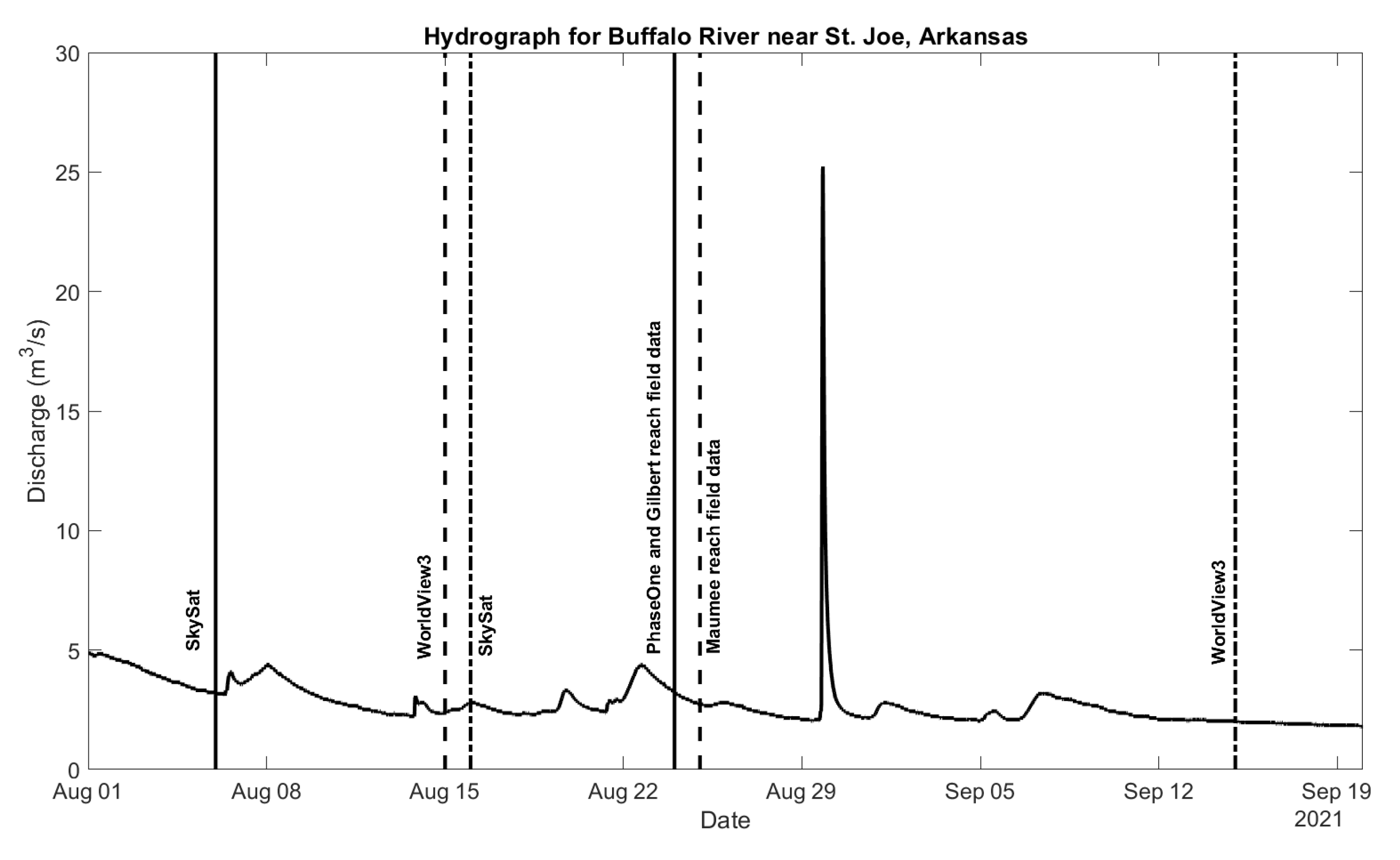
All of the field-based and remotely sensed data used in this study are publicly available through a data release by Legleiter and Hodges [27]. The main landing page for the data release has links to child items from which the individual datasets can be downloaded, along with corresponding metadata.

2.1. Study Area

This study focused on the Buffalo National River, a river-centered park with a history of benthic algal blooms. This river has experienced increases in blooms of filamentous green algae in recent years, with the affected river length expanding from approximately 32 km to 145 km between 2016 and 2018. In addition, the density of these blooms has reached unprecedented levels [28]. The spread of benthic algae is an important issue for the NPS because thick growths (Figure 1) can compromise, if not preclude, recreational activities such as boating, angling, and swimming. Park management has been focused on identifying these nuisance algal blooms by direct field observations and public reporting [7]. The latter has been encouraged by the park and made considerably easier by a web- or mobile device-based application developed for this purpose by the Arkansas Department of Environmental Quality [29].

The adverse effects of algal blooms on the health of the river ecosystem also are an important issue. Excessive growths of benthic algae limit the ability of fish to feed on benthic macroinvertebrates and access spawning substrates, thus placing at risk the 83 fish species found within the park; eight of these species already are listed as species of concern by the state of Arkansas [30]. The Buffalo National River also features two federally listed mussel species for which 113 km have been designated as critical habitat for the rabbitsfoot mussel [31]. However, mussel recovery efforts are undermined by the frequent occurrence of extensive benthic algal blooms that severely compromise habitat quality.

Multiple lines of evidence indicate that benthic algae pose a serious threat to the Buffalo River ecosystem. Moreover, the sizes of the algal blooms are increasing, and cyanotoxins have been detected for the first time. For example, ten of the thirteen sites sampled by NPS staff in 2018 reported saxitoxin, rather than microcystin, which is commonly the first cyanotoxin to be identified [5]. Although the levels observed were below consumption limits, recreational advisories have been issued intermittently. The potential for the blooms to become more severe has created a need to develop a capability to detect benthic algae rapidly and over a large area.

In terms of hydrology, the Buffalo River drains a densely forested watershed in northern Arkansas (Figure 2), a region of humid temperate climate [32]. The U.S. Geological Survey (USGS) operates a streamgage at St. Joe, where the contributing area is 2147 km² [33]. Portions of the channel are highly sinuous, with a series of tight, compound meander bends interspersed with relatively straight reaches. The river is bounded by limestone bluffs that rise up to 100 m above the narrow, confined valley floor. This type of bedrock is also exposed on the channel bottom in many locations [32].

This study focused on two sites, referred to as the Gilbert and Maumee reaches, located 6.7 km and 24.5 km downstream (east) from the gauge at St. Joe, respectively. The 510 m long Gilbert reach is shown in Figure 2f–h and has a straight planform with alternate bars and extensive bedrock control, including a constriction at the upstream end of our study site. The mean wetted channel width averaged over 11 transects was 40.7 m and the mean depth was 0.42 m at the time of field data collection. The Maumee reach is 276 m in length and arcs around a large gravel bar on the left bank of the river (viewed facing downstream). Eight transects were measured at this site, with a mean depth of 0.51 m and a mean wetted width of 33.5 m, but widths ranged from 23 m where the flow is constricted near the apex of the bend to 80 m above the bar (Figure 2a–c).

The water in the Buffalo River is generally clear throughout the summer months, with turbidity values typically less than 1 NTU during baseflow conditions [32]. Exceptions occur after rainstorms associated with frontal systems and dissipating tropical cyclones moving north from the Gulf of Mexico. These episodic events can increase turbidity and, if the flows reach a sufficient magnitude, can scour benthic algae from the streambed. Flow conditions in August and September of 2021 were typical to slightly above average for this time of year. The mean of the median daily streamflows observed between 6 August and 15 September at the St. Joe gauge over the 82-year period of record was 1.92 m³/s; the mean streamflow during our study was 2.74 m³/s [33]. A relatively small storm caused a slight rise in streamflow in the days prior to our field campaign, but the water had cleared by the time the airborne remote sensing flight occurred on August 24 (Figure 3). A larger event on August 29 led to an abrupt peak of 25.1 m³/s but the streamflow quickly returned to baseflow by the time the final satellite image was obtained on 15 September.

2.2. Field Data Collection

NPS personnel collected field data from the Gilbert and Maumee reaches on 24 and 25 August, respectively. At each site, regularly spaced transects (11 at Gilbert, 8 at Maumee) separated by approximately 50 m were established and measurements made at 18–20 points along each cross-section, accessed by wading the channel. The two key attributes observed at each point were the water depth and the percent cover of benthic algae on the streambed within a 0.3 m by 0.3 m area (quadrat) centered on the point. Depths were measured with a stadia rod and cover was estimated visually in 10% increments ranging from 0, where no algae was present, to 1, when the entire area was coated with algae. In addition, the UTM Zone 15N WGS84 coordinates of each point were established using a Leica Zeno GG04 Plus Global Navigation Satellite System (GNSS) receiver (Leica Geosystems, Heerbrugg, Switzerland; [34]). Horizontal positional accuracy for the 376 points recorded in the two reaches ranged from 0.03 m to 0.28 m, with a mean of 0.056 m.

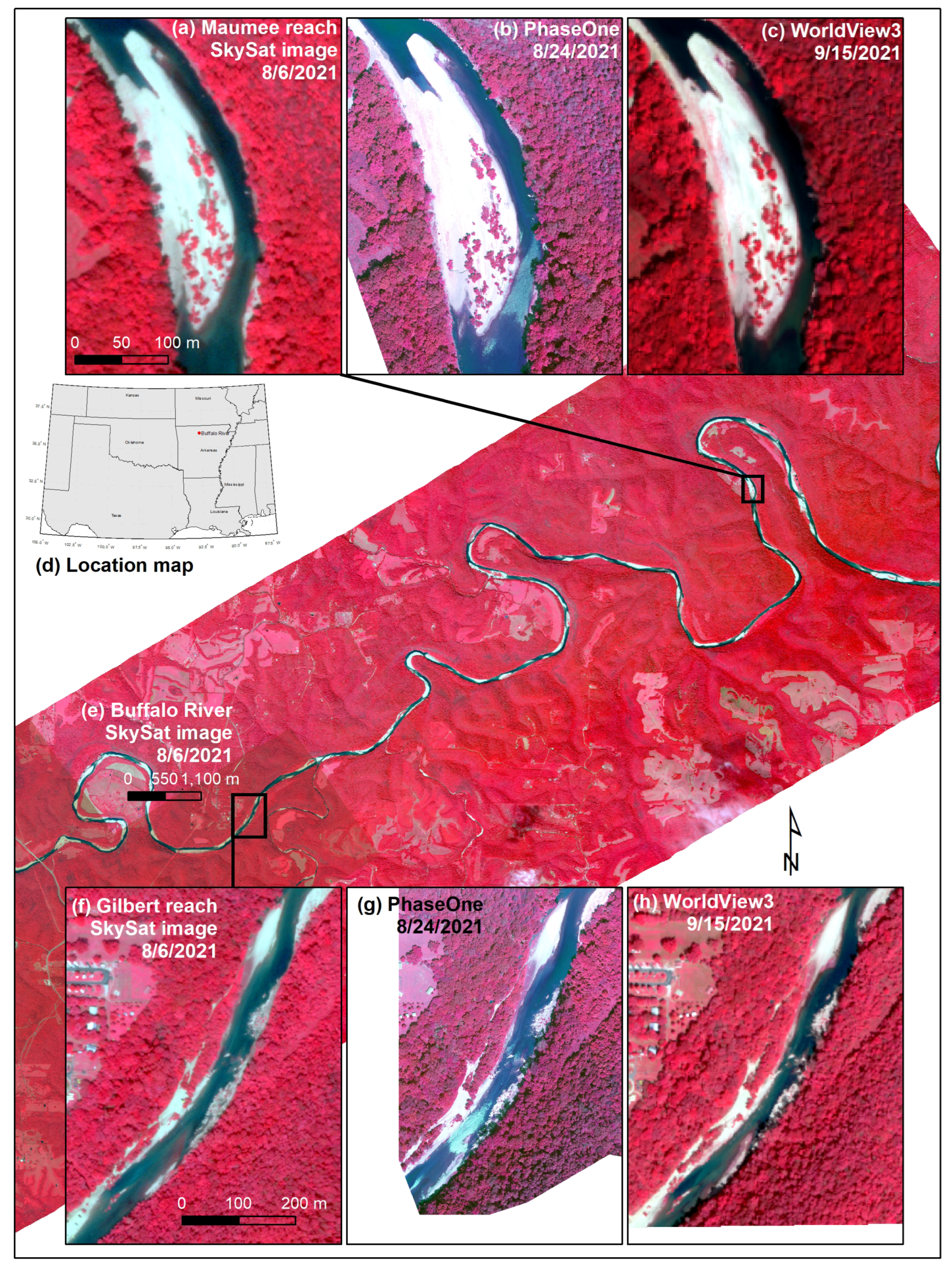
2.3. Remotely Sensed Data

To assess the potential utility of two readily available types of remotely sensed data for mapping benthic algae, we examined aerial photographs and satellite images spanning a range of spatial and spectral resolutions [27]. Characteristics of the three sensors used in this study are listed in

Table 1. Characteristics of sensors used in this study.

Sensor	Operator	Platform	Pixel Size (m)	Spectral Bands and Center Wavelengths (nm)
SkySat	Planet Labs	Satellite	0.5	4: B (482.5), G (555), R (650), NIR 1 (820)
WorldView3	DigitalGlobe	Satellite	1.81, 2 2	8: Coastal blue (426), B (481), G (547), Yellow (605), R (661), Red edge (724), NIR1 (832), NIR2 (948)
PhaseOne	USFWS 3	Aircraft	0.088	4: B (450), G (550), R (650), NIR (750)

¹ B = blue, G = green, R = red, NIR = near-infrared. ² The WorldView3 image acquired on 15 September 2021 had 1.81 m pixels, while that acquired on 15 August 2021 had 2 m pixels. ³ USFWS = United States Fish and Wildlife Service.

and example images from each instrument for the Gilbert and Maumee reaches are shown in Figure 2a–c,f–h, respectively. Note that the SkySat images from Planet Labs are commercially available to the public and were purchased for this study [35]. We obtained WorldView3 images at no cost through a contract between the federal government and DigitalGlobe, but other end users can also purchase this type of data directly from the vendor [36]. The aerial photographs were purchased through an interagency agreement between the USGS and the US Fish and Wildlife Service established for this study, but similar data could be acquired from private contractors.

Cloud-free, four-band, 0.5 m pixel images from SkySat were obtained on 6 and 16 August 2021, but the latter image did not encompass the Maumee reach. Eight-band images with 2 m and 1.81 m pixels were acquired by the WorldView3 satellite on 15 August and 15 September, respectively, and provided full coverage of both reaches. The WorldView3 sensor thus provided more spectral detail than SkySat but at the expense of a coarser spatial resolution. Images from both of these platforms were delivered with basic radiometric and geometric corrections applied. We did not attempt to account for atmospheric effects because each scene was analyzed individually (i.e., we did not apply depth retrieval relations or algal cover classifiers developed for one image to another image), implying that such standardization was not necessary. In addition, atmospheric correction over water bodies involves a number of unique challenges relative to more common terrestrial applications and can introduce uncertainties to image processing workflows even when using specialized algorithms developed for aquatic environments [37,38]. We therefore chose not to perform any kind of atmospheric correction due to the risk of introducing greater error to the remotely sensed data. The SkySat images were georeferenced and aligned closely with the field data from both reaches. For the WorldView3 datasets, however, the channel depicted in the images, as delivered, did not coincide with the points sampled in the field. We addressed this issue by using the SkySat images as a base and selecting tie points to transform the WorldView3 images to improve their coregistration with the field data. In addition, because the satellite images covered a much larger area than we required, the original scenes were cropped to produce subsets for the Gilbert and Maumee reaches.

In terms of the ability to resolve small-scale channel features, the most detailed remotely sensed data were acquired from a Quest Kodiak K100 aircraft operated by the US Fish and Wildlife Service (USFWS) on 24 August 2021, coincident with field data collection for the Gilbert reach. The plane was equipped with a PhaseOne iXURS-1000 four-band, 100 mega-pixel medium format digital camera attached to a SOMAG gyro-stabilized/vibration isolation sensor mount. A POS AV510 GNSS/IMU (inertial motion unit) navigational system recorded the position and orientation of the camera during the flight and enabled direct georeferencing (i.e., without image-to-image tie points). The original PhaseOne images were processed to generate orthophotos for the entire project area and delivered as individual tiles. The tiles covering the two study reaches were identified and combined into a separate mosaic for each reach. The resulting images had a pixel size of 0.088 m, an order of magnitude smaller than the satellite data.

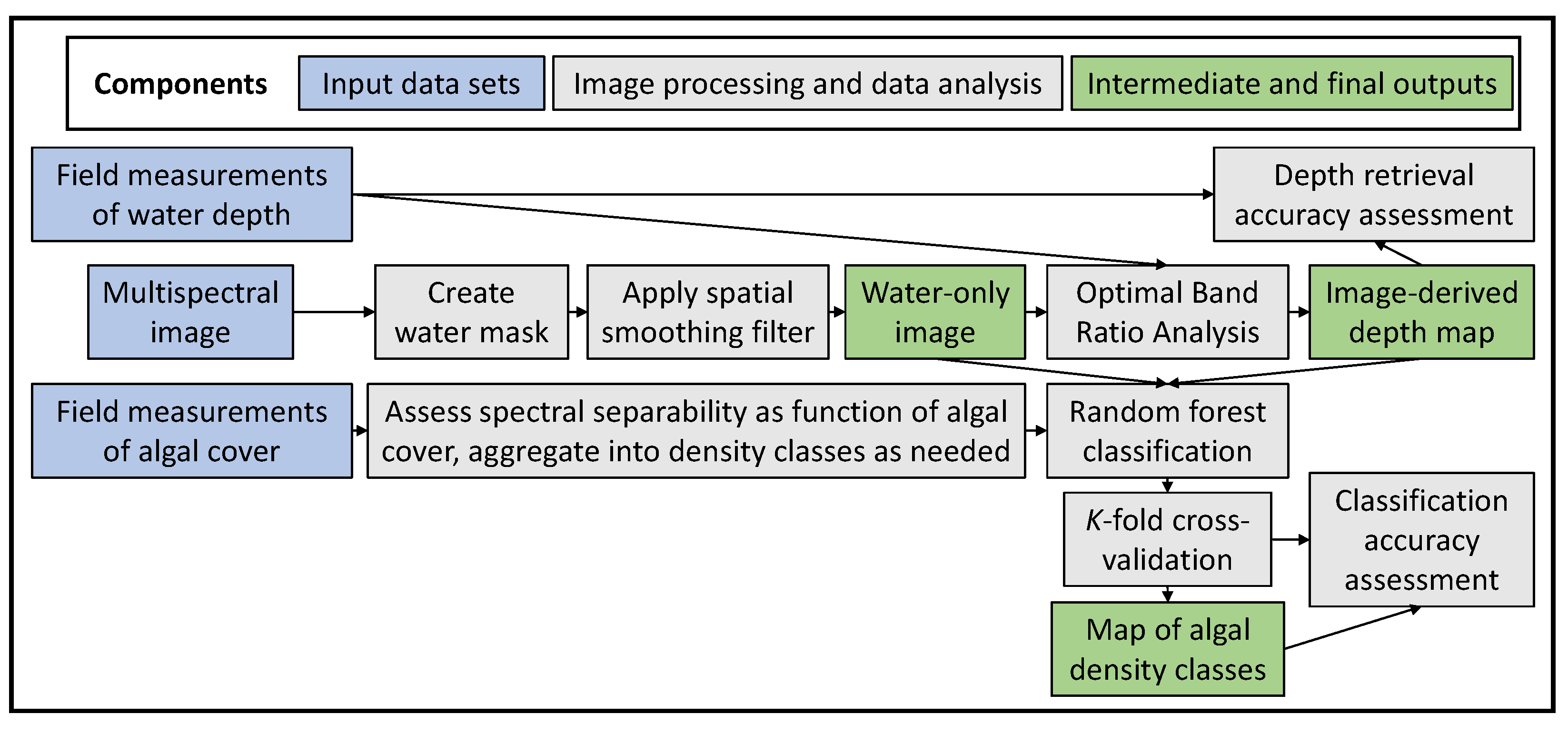
2.4. Workflow for Mapping Benthic Algal Blooms from Remotely Sensed Data

To achieve our goal of establishing a more efficient remote sensing approach to characterizing benthic algae in rivers, we developed the integrated image processing workflow summarized graphically in Figure 4. This framework consists of an initial preprocessing stage and then two primary components described in the subsections below: (1) estimating water depth via a spectrally based algorithm; (2) using a machine learning technique to classify algal density based on spectral information and image-derived depth estimates.

Preparing the orthophotos and satellite images for depth retrieval and algal classification involved isolating the wetted channel and spatially smoothing the data. For the SkySat and WorldView3 data, we used interactive contrast enhancement and image segmentation tools to identify a suitable near-infrared (NIR) band threshold to exclude terrestrial areas with higher reflectance and produce a mask that highlighted the relatively dark water, which absorbed strongly in this range of wavelengths. Although the PhaseOne camera also included an NIR band, this approach proved problematic when applied to the higher-resolution orthophotos due to extensive sun glint and shadows that had pixel values similar to water. We thus created masks for the PhaseOne images by manually digitizing wetted channel polygons to exclude areas of strong sun glint that would have prevented depth retrieval and algal classification. We applied the masks to produce water-only images that were, in turn, spatially smoothed using a $3\times 3$ pixel median filter that reduced noise and improved image texture. The masked, filtered water-only images then served as input to the depth retrieval and algal classification algorithms.

2.4.1. Spectrally Based Depth Retrieval

Estimating water depth from passive optical image data has a long history of application in marine (e.g., [39]), coastal (e.g., [23]), and, more recently, fluvial settings (e.g., [40]). Although some more sophisticated, lookup-table-based approaches involving radiative transfer modeling and carefully calibrated hyperspectral images have shown promise (e.g., [24]), empirical methods are practical and thus remain widely used, especially in rivers [41]. In this study, we applied one such technique, the optimal band ratio analysis (OBRA) algorithm introduced by Legleiter et al. [42] and refined by Legleiter and Harrison [43], to produce bathymetric maps of the Gilbert and Maumee reaches from each of the remotely sensed datasets described above. The OBRA framework has been applied successfully across a range of river environments [43] and is implemented within freely available software [44]. Legleiter et al. [42] and Legleiter and Harrison [43] contain additional detail; only a brief summary of OBRA is provided here.

In addition to a multi-band image, OBRA requires field measurements of water depth to calibrate a relationship between the image-derived quantity X and water depth d, where X is given by

$$X=ln{\displaystyle [}\frac{R\left({\lambda }_1\right)}{R\left({\lambda }_2\right)}{\displaystyle ]}$$

(1)

and $R\left({\lambda }_1\right)$ and $R\left({\lambda }_2\right)$ are reflectances, radiances, or raw digital numbers recorded in the numerator and denominator bands ${\lambda }_1$ and ${\lambda }_2$, respectively. Legleiter et al. [42] showed that under certain conditions, primarily shallow, clear water, and for an appropriate combination of wavelengths, defining X as a log-transformed band ratio can provide a linear relation between X and d. The OBRA algorithm proceeds by calculating values of X for all possible band combinations and then performing an X versus d regression for each pair of wavelengths. The optimal band ratio is that which yields the highest coefficient of determination, $R^2$. Because all of these regressions involve a single predictor variable, overfitting the model is not an issue.

In addition to identifying the best bands for retrieving water depth, OBRA also yields an empirical relation between X and d that can be applied throughout an image to produce a continuous depth map. Following Legleiter and Harrison [43], we used an exponential X versus d relation to avoid negative depth estimates or overpredictions of depth along shallow channel margins. In this study, we performed OBRA and generated depth maps for each type of image (air photos and multispectral images from two different satellites) for all dates available for each study site. Although the field measurements of water depth used for calibration were not collected on the same date as all of the images, we used the record of water level changes from the gauging station to account for these fluctuations and adjust the depth measurements accordingly.

After producing these bathymetric maps, we performed a thorough accuracy assessment of the image-derived depth estimates. This evaluation was based on 50% of the field measurements of water depth, sampled at random from the full dataset, that were excluded from the OBRA calibration process. For consistency with previous studies, we used the same metrics of performance as Legleiter and Harrison [43]: OBRA calibration $R^2$; visual inspection of depth maps; distributions of depth retrieval errors, defined as the field-measured depth minus the image-derived depth; and observed versus predicted (OP) regressions. In addition, we calculated the mean error and root mean square error (RMSE) to provide an indication of accuracy (bias) and precision both in absolute terms, with units of m, and in relative terms, normalizing by the mean of the field-based depth measurements.

2.4.2. Machine Learning-Based Classification of Benthic Algal Cover

To produce maps of benthic algae within each reach on each image date, we extracted spectra from the locations where measurements of algal cover were made in the field. Although these ground-based observations were obtained on only one day for each reach, we assumed that the conditions documented during our field surveys were representative of those captured in all of the images in our time series, despite the fact that some of the remotely sensed data was acquired up to 18 days before or 22 days after the field campaign. During this time, algal cover might have changed due to scouring by high flows, such as that which occurred on 29 August, and/or sloughing towards the end of the summer growth season. Moreover, because the field data were not truly continuous, with only 11 discrete values of percent cover (0 to 1 in increments of 0.1), we did not make numerical estimates of algal cover but rather treated this attribute as a categorical response variable and used a classification-based approach. To supplement the limited spectral information available, particularly for the four-band SkySat and PhaseOne images, we included the image-derived depth estimates obtained via OBRA as a predictor variable, in addition to all of the spectral bands, for assigning pixels to algal density categories. We performed a separate classification for each image of each reach, a total of nine datasets.

These classifications were produced using a supervised machine learning algorithm referred to as bagged trees or random forest [45]. Bagging is shorthand for bootstrap aggregation and refers to the process of compiling an ensemble of individual decision trees, each of which consists of a series of if–then statements (decision rules) to iteratively split the data until certain criteria are met (e.g., number of trees, number of splits, minimum number of observations per node). Every tree in the resulting ensemble, or bag, is grown using an independently drawn bootstrap replica of the input data. Observations not included in a given replica are considered “out of bag” for that particular tree and are used to assess the tree’s ability to classify observations not used for training. The tree bagger algorithm we used fits many simple trees and then combines them for prediction, with assignments based on the modal value of the observations for each terminal node. Advantages of the bagged tree technique include the ability to use different types of predictor variables without requiring data transformations, fit complex nonlinear relations, and automatically incorporate interactions among predictors. For all of these reasons, bagged trees, or random forest, classification have been used in a wide range of studies (e.g., [46]). In this study, we first augmented each of the original multi-band images with an additional “band” containing the depth estimates derived from that image, trained a bagged tree classifier for each dataset via k-fold validation (described below), and then applied the trained classifier to produce a classified map of algal density.

We used a k-fold cross-validation approach to both train the bagged tree classifiers and assess the accuracy of the resulting classifications. This method uses models (i.e., classifiers) trained on in-fold observations to predict the responses for out-of-fold observations. We used five folds for cross-validation, with the algorithm randomly assigning each observation into five equally sized groups. The training fold contains four of the groups (i.e., 80% of the data) and the test fold contains the other group (i.e., 20% of the data). For this study, the training and testing folds for the Gilbert reach thus consisted of 174 and 44 pixels, respectively, while the training and testing folds for the Maumee reach were composed of 126 and 32 pixels, respectively. The cross-validation then proceeds by (1) training the first model using the observations in the last four groups while reserving the observations from the first group for validation; (2) training the second model using the observations in the first and last three groups while reserving the observations in the second group for validation; and (3) processing the third through fifth models in a similar fashion. In short, the algorithm estimates a response for every observation using a model that was trained without that observation. The results of the cross-validation analysis of each classified image were summarized using confusion matrices, which tabulate the number of pixels in each true class assigned to each class by the bagged tree model. The rows of the matrix indicate the true class of each pixel, based on the field observations of algal percent cover, and the columns indicate the class to which the pixel was predicted to belong. The diagonal entries of the matrix thus represent correctly classified pixels while the off-diagonal elements correspond to classification errors. These errors represent confusion among algal density categories on the part of the bagged tree model, hence the term confusion matrix [47].

3. Results

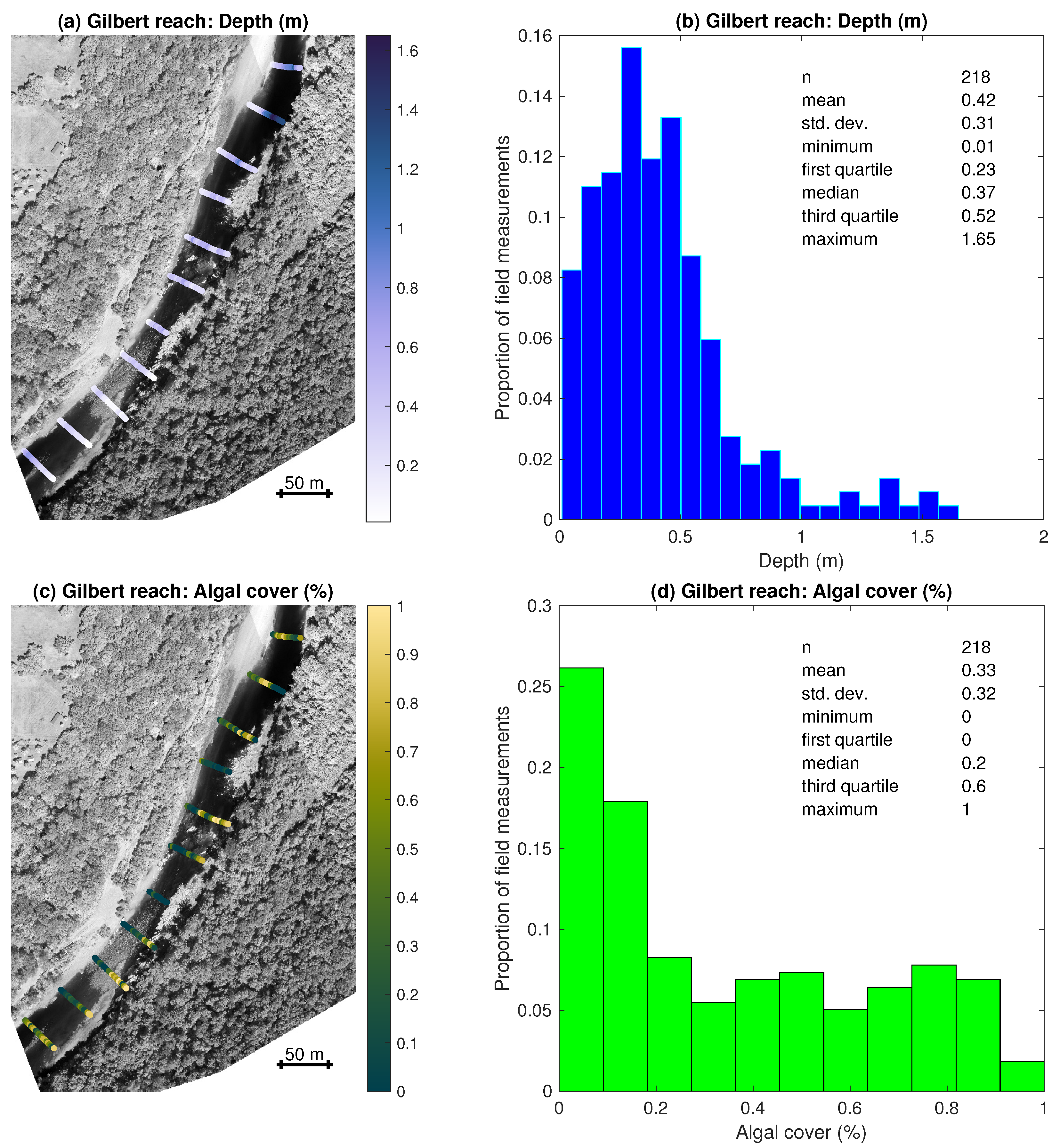
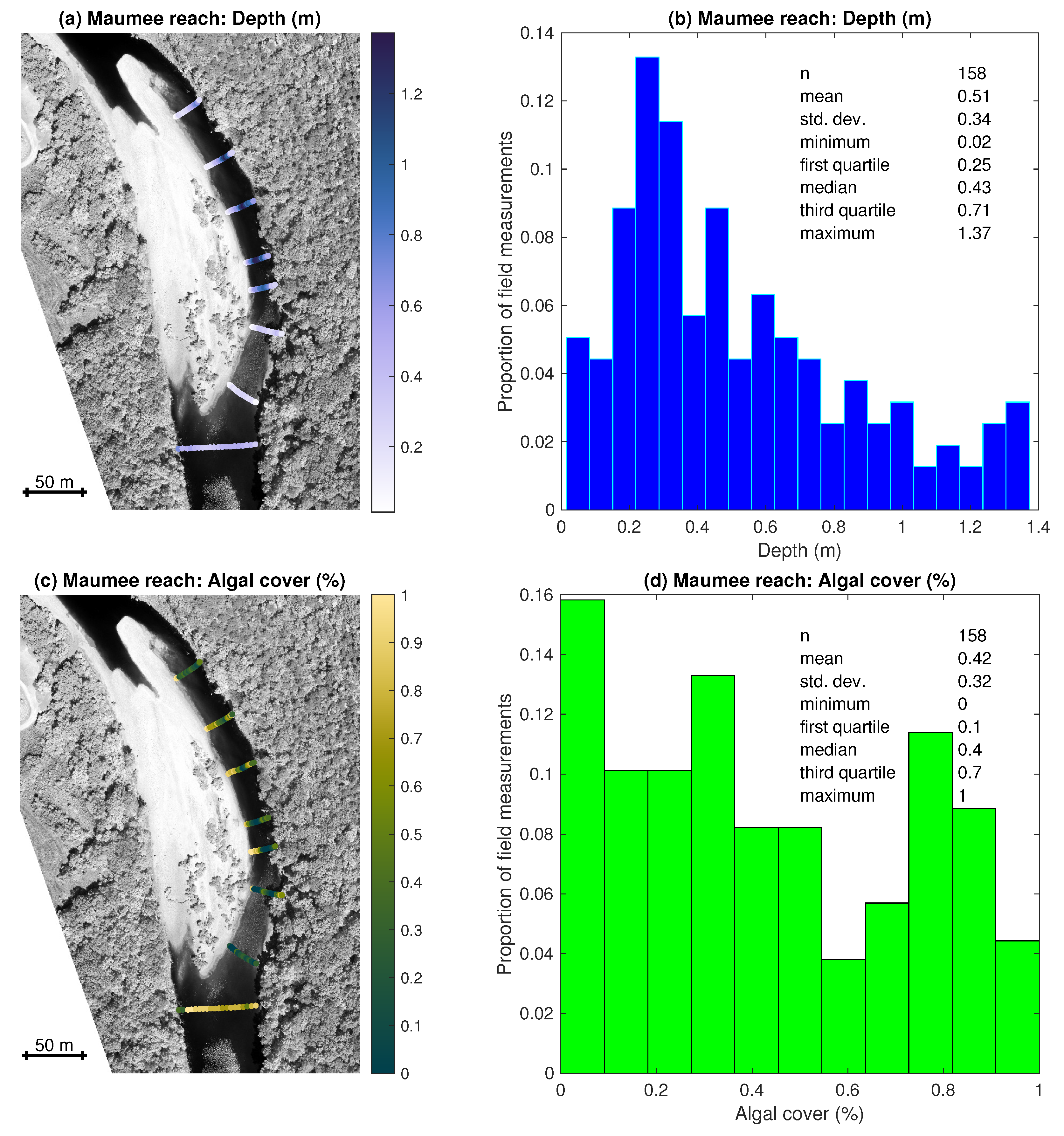
3.1. Field Observations of Depth and Algal Cover

The field observations of depth and algal cover in the Gilbert reach are summarized via the maps and histograms in Figure 5, while data from the Maumee reach are presented in Figure 6. Water depth and algal cover differed between the Gilbert and Maumee reaches. The Gilbert reach encompassed a straight section of the channel and had a mean depth of 0.42 m, shallower than the mean depth of 0.51 m observed in the Maumee reach. Although the maximum depth at Gilbert was greater (1.65 m) than that at Maumee (1.37 m), the relatively uniform, trapezoidal shape of the channel at Gilbert skewed the distribution toward the shallow end and led to a lower mean depth. Depths were more variable and greater on average at Maumee because the bar-pool morphology of the river at this site featured an asymmetric cross-sectional geometry with deeper water along the outer (right, or east) bank.

Our study reaches featured a number of species, including both green algae and toxigenic strains. Filamentous blooms have been observed along the Buffalo and the three main species of algae occurring in the river are Spirogyra, Oedogonium, and Cladophora. All levels of algal cover from 0 to 1 in increments of 0.1 were observed in both reaches, but the mean percent cover was lower in the Gilbert reach (0.33) than in the Maumee reach (0.42) (Figure 5 and Figure 6). Whereas over 25% of the locations sampled at Gilbert had no algae on the streambed and more than half had less than 30% coverage, the Maumee site had a more even distribution of algal cover and fewer points with no, or very little, benthic algae. Algae were most prevalent in shallow areas and less extensive in deeper portions of the channel in both reaches (Figure 5 and Figure 6).

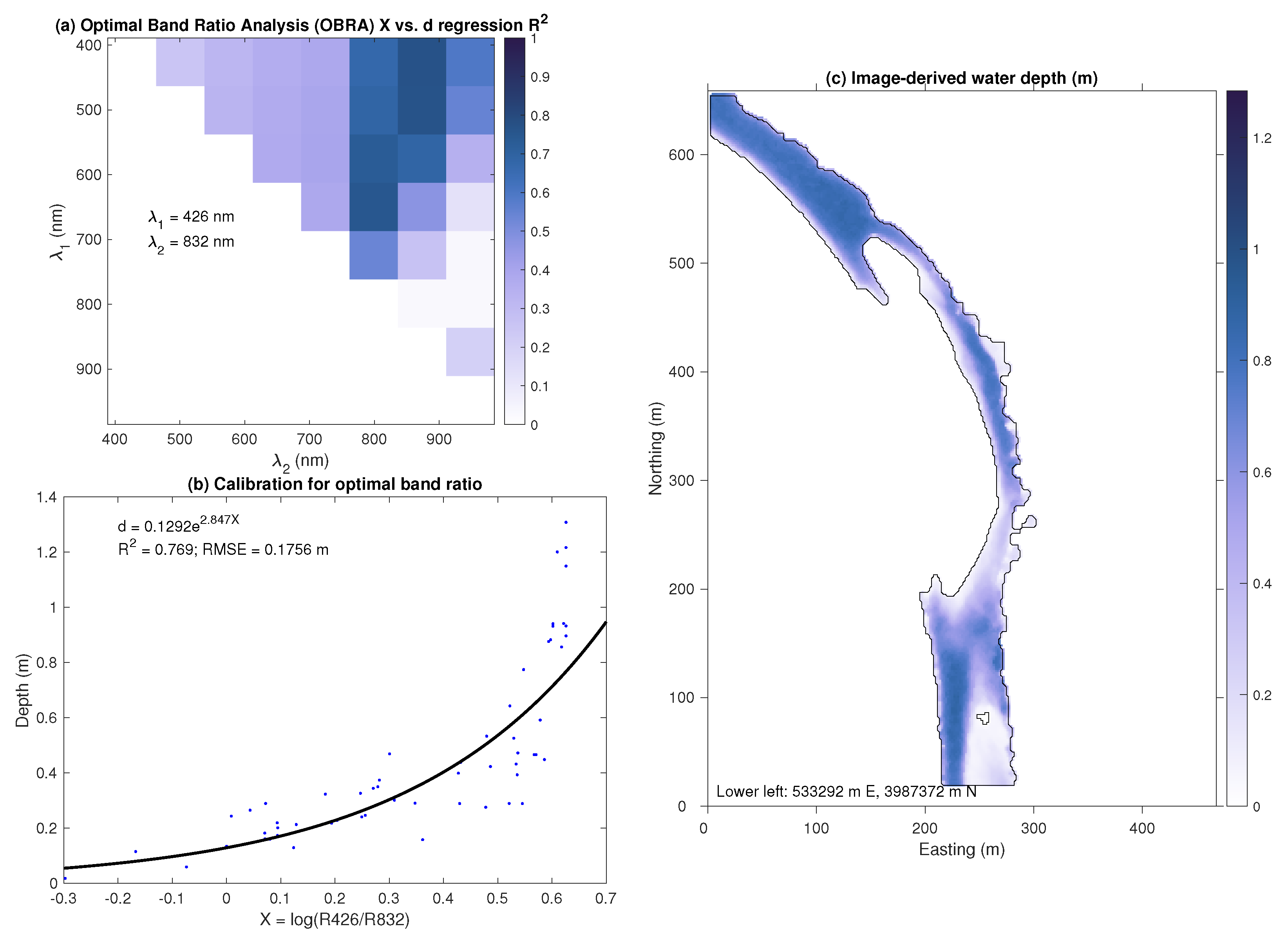
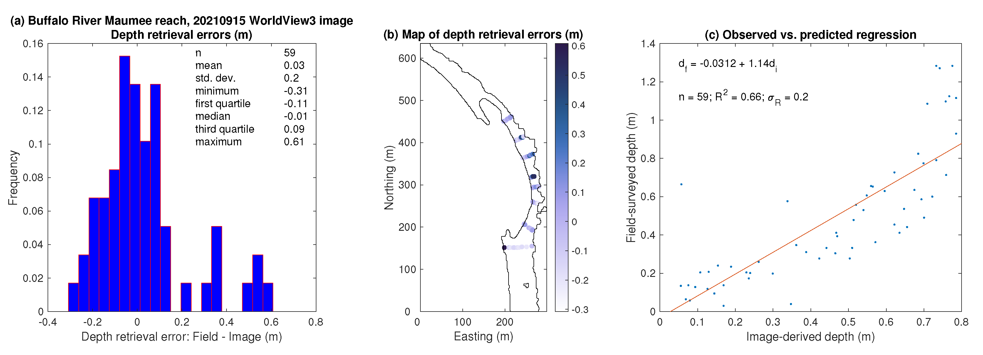
3.2. Bathymetric Mapping via OBRA

To capitalize on any such relationship between water depth and the spatial distribution of benthic algae, we applied the OBRA algorithm described in Section 2.4.1 to each image to create a series of depth maps. The resulting bathymetric information was then used as an additional predictor variable for classifying algal density. A representative example of the OBRA output from each of the nine images acquired for this study is shown in Figure 7a for the September 15 WorldView3 image of the Maumee reach. In this case, defining X using the coastal blue and NIR1 bands centered at 426 and 832 nm, respectively, yielded a strong exponential relationship with water depth ($R^2=0.77$). Although this particular combination of wavelengths was optimal, the vertical swath of dark blue tones in Figure 7a indicates that pairing either the red edge (724 nm) or NIR1 band as the denominator with any numerator band in the visible portion of the spectrum would have led to a correlation with depth that was nearly as high. This result is noteworthy because whereas the WorldView3 sensor has eight relatively narrow spectral bands, the SkySat and PhaseOne imaging systems have only four broader bands, with a single band in the NIR. Applying the calibrated OBRA relation shown in Figure 7b to the spatially filtered water-only image of the Maumee reach led to the bathymetric map in Figure 7c, which highlights deeper areas on the left (west) side of the channel at the upstream end of the reach (bottom of the image), along the right bank near the apex of the bend, and downstream of the bar. A large shallow riffle was located on the right side of the channel upstream of the bar where a pulse of gravel had been transported into the reach.

To assess the accuracy of the image-derived depth estimates, we used the field measurements set aside for validation, which comprised 50% of the total available, to calculate performance metrics including the OBRA and observed vs. predicted (OP) $R^2$ and the mean error and RMSE, as well as their normalized values, as proportions of the reach-averaged mean depth. The same dataset from the Maumee reach again serves as an example. In this case, the distribution of depth retrieval errors shown in Figure 8a is skewed toward positive values, with a mean error of 0.03 m indicating that depths tended to be underestimated from the image. The RMSE of 0.2 m was 36% of the mean depth measured in the field, implying that the image-derived depths were only moderately precise. Mapping these errors, as shown in Figure 8b, revealed that the largest positive errors occurred on the left edge of the channel at the beginning of the reach and along the outer bank through the bend where the greatest depths occurred. These underestimates of depth were greatest in areas with interference from terrestrial vegetation, mainly in the form of overhanging trees that obscured the channel or cast shadows. An observed vs. predicted regression of the depths measured in the field against those inferred from the image led to an $R^2$ of 0.66 and intercept and slope terms that differed from the ideal values of 0 and 1 that would imply perfect agreement. These results indicate that the OBRA relation did not perform quite as well when applied to data that were not used for calibration, largely because the estimated depths did not exceed 0.8 m even when the field-measured depths increased up to nearly 1.4 m. The primary factor limiting the accuracy of depth retrieval was the underprediction of depth in deeper areas of the channel, but variations in bottom composition, from bright limestone bedrock to dark algae-covered substrate, also might have played a role.

The results of this accuracy assessment for all nine of the images we processed are summarized in

Table 2. Summary of optimal band ratio analysis (OBRA) depth retrieval results for each image used in this study. OBRA $R^2$ values are based on a calibration subset of the field-based depth measurements and error statistics, and observed vs. predicted regressions are based on a separate subset of the field data set aside for validation.

Date	Sensor	Reach	OBRA ${\mathit{R}}^2$	Mean Error (m)	Normalized Mean Error	RMSE (m)	Normalized RMSE	Observed vs. Predicted ${\mathit{R}}^2$
6 August 2021	SkySat	Gilbert	0.50	0.03	0.065	0.22	0.478	0.51
15 August 2021	WorldView3	Gilbert	0.72	0.01	0.022	0.22	0.478	0.45
16 August 2021	SkySat	Gilbert	0.42	0.04	0.087	0.21	0.457	0.49
24 August 2021	PhaseOne	Gilbert	0.81	0	0.000	0.14	0.304	0.88
15 September 2021	WorldView3	Gilbert	0.72	0.03	0.065	0.2	0.435	0.77
6 August 2021	SkySat	Maumee	0.67	0.09	0.161	0.24	0.429	0.58
15 August 2021	WorldView3	Maumee	0.85	−0.03	−0.054	0.17	0.304	0.67
24 August 2021	PhaseOne	Maumee	0.90	0.01	0.018	0.19	0.339	0.73
15 September 2021	WorldView3	Maumee	0.77	0.03	0.054	0.2	0.357	0.66

. OBRA $R^2$ values based on the calibration subset of the field-based depth measurements ranged from 0.42 to 0.90, with the four-band, 0.5 m SkySat images yielding the lowest $R^2$ and the airborne data with the highest spatial resolution providing the most reliable depth estimates. The availability of eight spectral bands for WorldView3 led to an intermediate level of performance despite the sensor’s relatively coarse ∼2 m pixels. In all but one case, the mean depth retrieval error, based on the subset of the field dataset aside for validation, was positive, implying that image-derived depths tended to be biased shallow, relative to the field measurements, by as little as 0.01 m for the PhaseOne image of the Maumee reach or as much as 0.09 m for the SkySat image of this site. These errors represent 1.8% and 16.1% of the mean of the depths measured in the field in this reach, implying that the spectrally based depth estimates were reasonably accurate. RMSE values varied from 0.14 m to 0.24 m and were lowest for the PhaseOne orthophotos and highest for the SkySat scenes. The corresponding normalized RMSE values of 30.4% to 42.9% indicate that the image-derived depths were only moderately precise. OP $R^2$ values differed from the OBRA $R^2$ values due to sampling fluctuations in the allocation of field observations to the calibration and validation subsets but confirmed the superior performance of the PhaseOne imaging system, with an OP $R^2$ as high as 0.88 for the Gilbert reach. Overall, these results confirmed that reliable estimates of river bathymetry could be derived from readily available image data to provide an additional source of information for mapping benthic algae in shallow, clear-flowing streams with depths up to approximately 2 m.

3.3. Classification and Mapping of Benthic Algae

As an initial step toward our goal of mapping spatial variations in coverage of the streambed by benthic algae, we examined spectra extracted from image pixels colocated with our ground-based measurements. These field data consisted of visual estimates of percent cover ranging from 0 to 1 in increments of 0.1, so we computed mean spectra for each of these levels of coverage. As an example, the resulting averaged spectra for the WorldView3 image of the Gilbert Reach acquired on 15 September are shown in Figure 9a. The vertical axis of this figure is in units of digital numbers, which are proportional to the brightness of an image pixel and thus the reflectance of the surface. This type of information can be used to distinguish among different types of material, or, in this case, levels of algal density. Note also that this type of spectral analysis is distinct from and unrelated to the frequency spectra often used to examine time series. Although a tendency for pixels with greater algal cover to have lower reflectances in most bands was evident, this trend was not consistent across the spectrum and the differences between percent cover levels were slight. In general, all of the images we examined for both reaches lacked clear spectral distinctions between the original 11 levels of algal cover.

Given the ordinal nature of the original field data and the subtle spectral differences between percent cover levels, we aggregated the field observations into four generalized classes of algal density, coded as 0 for none, 1 for low (percent cover from 0.1–0.3), 2 for medium (0.4–0.6), and 3 for high (0.7–1). The aggregated mean spectra for the September 15 WorldView3 image of the Gilbert reach for the four algal density classes are shown in Figure 9b. Pixels with a greater density of benthic algae (i.e., the medium and high classes) are more distinct from those with little or no algae, particularly in the yellow, red, and NIR bands between 600 and 750 nm. Overall, however, the differences between even these broader categories were neither large nor consistent across all of the images we examined, implying that classifying algal density based on these image spectra could be challenging.

To provide some additional information for distinguishing among the four categories of algal density, we included the depth map derived from each image as a predictor variable along with the original spectral bands. We then applied the bagged tree algorithm described in Section 2.4.2 to each dataset to produce a series of algal density classifications for the Gilbert Reach, shown in Figure 10, and the Maumee reach, presented in Figure 11. For both sites, the classified maps were somewhat pixelated in appearance, and the spatial pattern of areas with no algae or a low, medium, or high density of algae on the streambed varied over time, but some consistent patterns also emerged. For example, in the Gilbert Reach, a persistent zone of high algal density occurred on the right (east) side of the channel downstream of a partially vegetated bar attached to the right bank. Further upstream, above this bar, an area with either no benthic algae or a low density was found along the left (west) side of the river for the latter four image dates. For the Maumee Reach, zones of high algal density were found spanning the full channel width upstream of the point bar on the left bank and along the bar’s shallow margins. The gap in Figure 11c was a consequence of sun glint in the PhaseOne image, evident as bright water in Figure 2b, that precluded depth retrieval and classification.

To assess the accuracy of the algal density classifications, we used a five-fold cross-validation technique that involved assigning each pixel to a class using a bagged tree model that was trained on a dataset that did not include that particular pixel, as described in Section 2.4.2. The results of this analysis were summarized using confusion matrices such as the example shown in Figure 12 for the WorldView3 image of the Maumee reach acquired on 15 September 2021. In Figure 12, the confusion matrix has been row-normalized (i.e., by the total number of pixels in each true class) so that the number of pixels predicted to be in each class is given as a percentage of the true number of pixels in that class; each row of the matrix thus sums to one. In addition, the matrix cells are colored such that darker green tones on the diagonal depict a greater proportion of correctly classified pixels, while the more saturated orange colors off the diagonal depict predicted classes to which a greater proportion of pixels were erroneously assigned. To the right of the main confusion matrix in Figure 12 is a distilled summary in which the true positive rate for a given algal density class (i.e., the proportion of pixels in that true class that were correctly assigned) is represented by the left column and the corresponding false negative rate (i.e., the proportion of pixels in that true class that were incorrectly predicted to be in another class) by the right column. The false negative rate is also known as the omission error and subtracting the omission error from 100% yields the producer’s accuracy (i.e., true positive rate). Similarly, the false positive error rate, or commission error, is used to obtain the user’s accuracy by subtracting the commission error from 100%. These metrics are summarized in

Table 3. Producer’s and user’s accuracies for each algal density class for the September 15 WorldView3 image of the Maumee reach of the Buffalo River example featured in Figure 12.

Algal Density Class	Producer’s Accuracy	User’s Accuracy
None	54.5	63.1
Low	66	61.1
Medium	37.9	45.8
High	86.5	78.7

for each class for the Maumee reach example highlighted in Figure 12.

For the highest algal density class, coded as 3, 86% of the pixels mapped as high density in the field were correctly classified as such from the image, 7% of these pixels were mistaken as medium density, and another 7% as low density. The true positive rate was thus 86% and the false negative rate was $7\%+7\%=14\%$. For this image of the Maumee reach, areas with no benthic algae or only a low algal density (coded as 0 and 1, respectively) were generally classified accurately, with true positive rates of 54.5% and 66%, respectively. The intermediate algal density class (coded as 2), however, was correctly classified for only 37.9% of the pixels mapped as medium in the field, with just as many of these pixels predicted to be in the low-density class and another 20.7% assigned to the high-density class. Similarly, over 31% of the pixels mapped as having no algae were incorrectly inferred to have a low density of algae on the streambed. The results presented in Figure 12 are for a single image used as an example but are representative of the confusion matrices we produced from the other images we analyzed. In general, classifications were not highly accurate, with a large proportion of pixels erroneously assigned to algal density categories other than that as which they were mapped in the field.

Our assessment of the accuracy of the algal density classifications produced from all nine Buffalo River images is summarized in

Table 4. Accuracy assessment of Buffalo River algal classifications based on five-fold cross-validation.

Reach	Date	Sensor	Overall Accuracy without Depth (%)	Overall Accuracy with Depth (%)
Gilbert	6 August 2021	SkySat	38.5	37.6
Gilbert	15 August 2021	WorldView3	47.1	54.4
Gilbert	16 August 2021	SkySat	39	38.3
Gilbert	24 August 2021	PhaseOne	47.8	49
Gilbert	15 September 2021	WorldView3	50.2	54.3
Maumee	6 August 2021	SkySat	49.2	55.4
Maumee	15 August 2021	WorldView3	59.3	62
Maumee	24 August 2021	PhaseOne	50	63.7
Maumee	15 September 2021	WorldView3	61.1	64.6

. To evaluate whether and to what extent incorporating bathymetric information might improve performance, we produced bagged tree classifications both with and without image-derived depth estimates as an additional predictor variable complementing the original spectral bands. In seven out of nine cases, the overall accuracy, defined as the number of correctly classified pixels (i.e., the sum of the diagonal entries of the confusion matrix) divided by the total number of pixels in the image, was greater when depth was included in the classification process. For the PhaseOne image of the Maumee reach, adding bathymetry to the dataset improved the overall accuracy from 50% to 63.7%, but for most of the images, the gains were more modest and classifications based on the SkySat images of the Gilbert reach were actually slightly more accurate without depth. More importantly, even when depth was included, overall classification accuracies remained low, ranging from as little as 37.6% to a maximum of 64.6%. Accuracies were higher for the Maumee reach than for Gilbert and tended to increase over time at both sites. The two least accurate classifications were derived from SkySat images of the Gilbert reach and this sensor also underperformed relative to the PhaseOne and WorldView3 instruments at the Maumee site. Overall, the results of this study suggested that, for the conditions observed along the Buffalo River at the time the images were acquired, mapping benthic algae from readily available remotely sensed data using established depth retrieval and image classification methods was more difficult than anticipated.

4. Discussion

4.1. Monitoring Benthic Algae via Remote Sensing

Benthic algal blooms in clear-flowing streams can alter the structure and function of aquatic food webs through various trophic cascades. In addition, such blooms are often highly visible and, in the context of U.S. national parks, lead to negative visitor feedback. More generally, increases in the frequency and/or extent of algal blooms in nutrient-poor water bodies could be an indicator of larger-scale, longer-term environmental change [3,48]. An improved capacity to detect, map, and monitor HABs via remote sensing could enable the formation of HABs to be identified early on and thus allow public warnings to be issued in a timely manner when necessary.

In the short term, developing remote sensing techniques for mapping benthic algae could guide field sampling, facilitate monitoring, and help to promptly inform public health advisories. Even if classification accuracies are modest, the workflow outlined herein would enable data collection over much larger areas, including sites in very remote locations. This strategy thus would allow some monitoring to occur even in reaches that cannot be visited by field crews or are checked only once every three to five years, assuming that field observations from more accessible intensive study reaches could be used to train a classifier applicable to much longer river segments. In addition, remote sensing could help to identify areas or hot spots where nitrate, for example, enters a river, such as confluence zones where tributary inputs might spur excessive growth of benthic algae. Over a longer time period, employing a synoptic remote sensing approach in rivers experiencing algal blooms might yield insight into causative factors and thus point toward potential mitigation strategies. Conversely, continued reliance on cumbersome field-based monitoring might have a range of undesirable consequences as the adverse effects of algal blooms on the health of both humans and ecosystems become more pronounced. Without greater understanding of the drivers involved in their formation, the spread of benthic algal blooms could continue unabated.

In this paper we presented results from a case study of the Buffalo National River designed to assess the potential to map benthic algal blooms from different kinds of readily available remotely sensed data. While the Buffalo River was of interest in its own right and provided an appropriate venue for development and testing, the broader impetus for this study was the increasingly widespread occurrence of benthic algal blooms in not only national parks throughout the US but rivers worldwide. This trend creates a compelling need to establish improved methods of detecting blooms, mapping their spatial extent, and monitoring their evolution over time. Remote sensing is uniquely capable of satisfying these requirements and the framework outlined herein could help to identify blooms and quantify their spatial and temporal variability. Ultimately, this approach might advance our knowledge of the environmental factors driving HAB formation and guide management efforts. However, if efficient, reliable tools to identify and map blooms are not developed soon, continued degradation of riverine resources will likely lead to compromised aquatic ecosystems and recreational opportunities. This study thus aimed to not only improve our understanding of benthic algal blooms in the specific context of the Buffalo National River but also assess the potential utility of remote sensing for examining algae-related issues throughout the U.S. NPS network and clear-flowing rivers around the world.

To illustrate how this approach might be applied in practice, we produced a series of classified maps of algal density for two reaches of the Buffalo River from satellite images and orthophotos acquired in August and September of 2021 (Figure 10 and Figure 11). We then used this sequence to examine the dynamics of benthic algae during the 40-day time period. For the Gilbert reach, an extensive area of high algal density at the downstream (northern) end of the reach identified in the images from 6 and 15 August (Figure 10a,b) disappeared by 24 August and then partially reestablished along the right (east) side of the channel by 15 September. Conversely, an area with little or no benthic algal cover at the upstream end of the reach that was evident in the first two images had been colonized by a high density of algae by the time the final image in the time series was acquired. For the Maumee site, a similar pattern occurred, with the broad zone of high algal density found at the lower (northern) end of the reach on August 6 being replaced by much more sparse algal cover in the latter three maps shown in Figure 11b–d. Algal density decreased in the middle of the channel at the upper end of the reach between 15 August and 15 September. Because our image time series did not more closely bracket the high flow event on 29 August, we were unable to discern whether the loss of algae toward the end of summer was due to a punctuated sloughing event or a more gradual process. This type of information would be important for resource managers because sloughing events associated with high flows tend to leave algal mats in eddies that can lead to greater exposure to the public.

To summarize these observations and obtain a reach-scale perspective on algal dynamics, we plotted the proportion of each study site assigned to each of the four algal density classes as a function of time (Figure 13). For the Gilbert reach, no clear, consistent trends emerged, with the abundance of all four classes fluctuating throughout the time series. Whereas the none, low, and high categories remained similar in extent at the beginning and end of the sequence, the proportion of the reach classified as medium algal density decreased over the 40-day time period. Both the medium- and high-density classes increased between 24 August and 15 September while low and medium decreased, suggesting that benthic algae might have become more well-established later in the summer. This inference was substantiated by qualitative field reconnaissance of the Gilbert reach in late September. Another plausible explanation is that the species present within the reach changed from early to late summer. Changes in flow can precipitate shifts in species composition, with taxa that can attach tightly to the streambed giving way to species that are only loosely attached and thus slough much more easily. For the Maumee site, the proportion of the reach classified as high algal density decreased over time while the low-density class increased and the total area in the none and medium classes remained stable even as the spatial pattern shifted. In any case, this type of analysis, supported by repeat imaging, could help to detect potentially harmful algal blooms at an early stage of development and thus enable timely management actions to be taken.

4.2. Limitations and Lessons Learned

Although both the need for improved methods of mapping benthic algae and the potential of remote sensing to contribute in this context are clear, this initial investigation of the feasibility of such an approach was limited in several respects. For example, we focused on a single river over a brief, 40-day period as a proof-of-concept case study and our results fell short of demonstrating a successful, satisfying application of the workflow outlined in Figure 4. Although we made detailed field measurements from two distinct reaches of the Buffalo River and acquired images on five dates using two satellite-based sensors and an airborne camera, this dataset might not have been representative of conditions on the Buffalo River, let alone other streams elsewhere. This study took place during a season (late summer 2021) in which benthic algae were not as well established along the Buffalo as in recent years; our timing was not fortuitous. Moreover, our analysis rested upon the assumption that the field observations made on a single day for each reach remained constant and thus could be applied to images acquired up to 18 days before or 21 days after the field survey. However, subsequent site visits after the last satellite image was obtained indicated that substantial algal development had occurred, casting doubt upon this assumption. One reason why algal density classification accuracies improved over time could be that benthic algae developed as the growing season went on, making their spectral signal more pronounced in the later images. If the spatial pattern of algal cover we documented in the field was consistent but the density of algae at a given location increased over time, the field data used to train the classifiers might have been representative in a relative sense but not necessarily in absolute terms. We do not have the repeated field surveys needed to test this possibility, but these changes in algal cover might have caused our assessments of classification accuracy to be overly pessimistic. For example, algal cover on the Maumee Reach was observed to have increased between 25 August, when the field data were collected, and 15 September, when the last WorldView3 image was acquired. As a result, the areas that were considered misclassified as low rather than none (i.e., the 31.8% off-diagonal entry in Figure 12) might not have been incorrect if algae had in fact colonized a large portion of the area mapped as none in the field several weeks prior. In this case, the accuracy of the classification might have been better than suggested by the confusion matrix in Figure 12 (i.e., up to 54.5% + 31.8% of the pixels mapped as none might have been correctly classified). Similarly, for locations that were classified as low but mapped as medium in the field, potential undersampling of medium levels of algal cover, as reported by the field crew, might have increased the likelihood of these areas being misclassified. These issues suggest that our classifications of algal density might have been more accurate than indicated by the accuracy assessments we performed. Collecting field data at the same time images are acquired would reduce this kind of ambiguity and thus enable more robust and informative accuracy assessment.

In addition to the limitations associated with this particular study, we also identified several more general issues that merit further consideration. Some of the lessons we learned have broader relevance and could guide further efforts to characterize benthic algae via remote sensing. For example, we purchased the SkySat images from Planet Labs, contracted with the USFWS to collect the aerial photographs, and were only able to obtain WorldView3 images at no cost through a special arrangement between the federal government and the vendor. A broader end user community would need to buy all of these data products, an important caveat implying that only those organizations that can afford suitable remotely sensed data would be able to apply this approach. In addition, sensor characteristics are likely to play a critical role in algal mapping, primarily the spatial and spectral resolution of the imaging system. We hypothesize that the main factor leading to the modest classification accuracies reported herein was the limited spectral information content of the images we used. The SkySat and PhaseOne instruments had only four bands, with one in the NIR, while WorldView3 had eight bands, with three in the NIR. Even greater spectral detail is needed to discern the narrow, often subtle absorption features associated with chlorophyll and other algal pigments. For example, the nearly continuous field spectra used by Legleiter et al. [21] allowed these authors to identify specific wavelengths where differences between levels of algal cover were most pronounced, which led to higher algal density classification accuracies approaching 80%. Our results suggest that spatial resolution is of secondary importance, as a smaller pixel size did not appear to compensate for inadequate spectral detail. Although images with very high spatial resolution, such as the 0.088 m orthophotos used in this study, might be helpful for discerning fine scale patterns of algal cover, the utility of such data could be compromised by the paucity of bands on sensors such as SkySat and the PhaseOne camera.

A number of other factors could constrain, if not prohibit, the use of remote sensing to characterize benthic algae. For example, in addition to the spectral and spatial resolution of the imaging system, one must also consider the platform from which the sensor is deployed. Although satellites can be tasked for specific project areas, coordination with field-based sampling is problematic because even if a specific date is requested, there is no guarantee that a cloud-free image will actually be acquired on that date. Dispatching a field crew as soon as possible after a suitable image is obtained might be a reasonable strategy but would require placing personnel on standby and could lead to frustrating delays. Airborne data collection allows for closer coordination but typically involves working with flight contractors that can be difficult to schedule in advance. Moreover, in our experience, high spatial resolution aerial photography such as that used in this study is more susceptible to sun glint that can compromise or preclude algal mapping. For certain combinations of sensor view angle and solar geometry, sun glint can be pervasive and careful flight planning to avoid these conditions is essential [49,50].

Regardless of the sensor and platform, environmental factors will limit the utility of remote sensing in many cases. To detect benthic algae, the bottom must be clearly visible in the images, a condition satisfied only in relatively clear-flowing, shallow streams. This approach is not applicable to larger, deeper, and/or more turbid rivers, where underwater acoustic devices such as multibeam echosounders might provide useful data for mapping submerged aquatic vegetation [51,52]. Because the range of detectable depths depends on both the radiometric resolution of the imaging system and the optical characteristics of a particular river of interest, establishing general guidelines on the sizes and types of channels where passive optical depth retrieval and substrate mapping might be feasible is difficult. However, Legleiter and Fosness [53] provide a framework for detecting optically deep water and thus defining the limits of this approach. Even large rivers often have shallow areas and riffles, or at least channel margins, with suitable habitat for benthic algae that would be amenable to examination via the remote sensing methods described herein. Riparian vegetation extending over the channel, as well as shadows, can also obscure the view from above and would likely preclude applying this approach to small first- and second-order streams. The dynamic, often patchy nature of benthic algae creates additional complications, as the rapid onset, growth, and decay of algal blooms places a premium on timely field sampling and, if at all possible, simultaneous image acquisition. Similarly, precise spatial coregistration between ground-based observations and remotely sensed datasets is essential. Finally, the subjective, semiquantitative methods used to characterize algae in the field lead to “ground truth” that might not be entirely reliable, particularly when used as training data for image classification. In addition, partitioning the continuous distribution of algal cover into discrete categories, or even ordinal ranks, is an arbitrary exercise and might not be consistent and informative enough to support the intended management applications.

4.3. Advancing the Remote Sensing of Benthic Algae

While the problems described in the preceding section must be acknowledged and addressed to the greatest extent possible, we remain cautiously optimistic regarding the potential for remote sensing of benthic algae and believe that further research is warranted. For example, this approach could yield insight on potential factors driving benthic algal blooms, including nutrient enrichment, changing hydrology, and a warming climate [54,55]. Because spectral resolution was identified as a key limiting factor in this study, adopting hyperspectral approaches capable of exploiting the absorption features characteristic of algae could improve our ability to characterize blooms. A precedent for this type of work was established by Legleiter et al. [21], and collecting ground-based measurements of spectral reflectance along with direct, simultaneous, colocated observations of algal cover across a broad range of river environments could be highly informative. Such a dataset could allow specific wavelengths, spectral indices, and possibly other metrics strongly correlated with algal density to be identified. Additionally, substantial progress might be made by moving beyond ordinal rankings of algal density and instead using measurements of algal biomass to support a more quantitative approach. Although pursuing this objective would involve laborious field sample collection and processing, the effort has the potential to produce continuous maps of benthic algae rather than continuing to rely upon discrete classifications.

A more ambitious goal could be to infer not only the presence and abundance of benthic algae but also their taxonomic composition. Such efforts are already underway in the marine environment, where distinguishing between seagrasses and macroalgae is becoming a fundamental aspect of habitat mapping [23,24]. This additional information could be highly valuable because different types of algae have a variety of effects on infrastructure (e.g., drinking water intakes) and human health and play diverse roles in aquatic ecosystems. Not all algae are harmful, but a capacity to identify those that are potentially toxic could more effectively inform management actions. A plausible way forward was pioneered by Paine et al. [56] and Slonecker et al. [57], who showed that reflectance spectra measured in a lab while viewing algal samples under a microscope could be used to distinguish between taxa. Slonecker et al. [58] have already published a spectral library consisting of 13 genera that is freely available to support this type of work; these authors plan to expand the library to include additional taxa [57]. A logical next step toward a hyperspectral approach to algal mapping might involve acquiring hyperspectral images from a UAS in coordination with the collection of field samples processed for biomass and taxonomy. This strategy could take advantage of the greater flexibility in deployment of UAS relative to satellites or conventional aircraft. Although the spatial coverage might be less extensive, UAS are more appropriate for local, reach-scale studies and also provide higher spatial resolution. If these UAS-based proof-of-concept investigations produce encouraging results, hyperspectral image data could be acquired from helicopters or fixed-wing aircraft to scale up to longer river segments or entire watersheds and thus more fully capitalize upon the potential to characterize benthic algae via remote sensing.

5. Conclusions

Blooms of benthic algae have become increasingly common not only in many of the parks managed by the NPS but also, presumably, in rivers worldwide. Improved methods of characterizing these blooms are thus needed to better understand their dynamics, identify causative factors, and develop effective management strategies for mitigating their adverse effects on human and ecosystem health. Remote sensing techniques have proven useful for monitoring algae at the surface of large lakes and reservoirs but have seldom been applied to examine bottom-attached algae in riverine environments. In this study, we evaluated the feasibility of mapping variations in benthic algal coverage from aerial photographs and satellite images. Our initial proof-of-concept investigation focused on the Buffalo National River and involved developing a workflow to incorporate information on water depth into a machine learning algorithm for classifying and mapping different levels of algal density. The accuracy of the resulting classifications was then assessed using field observations of algal percent cover. The results of this analysis support the following principal conclusions:

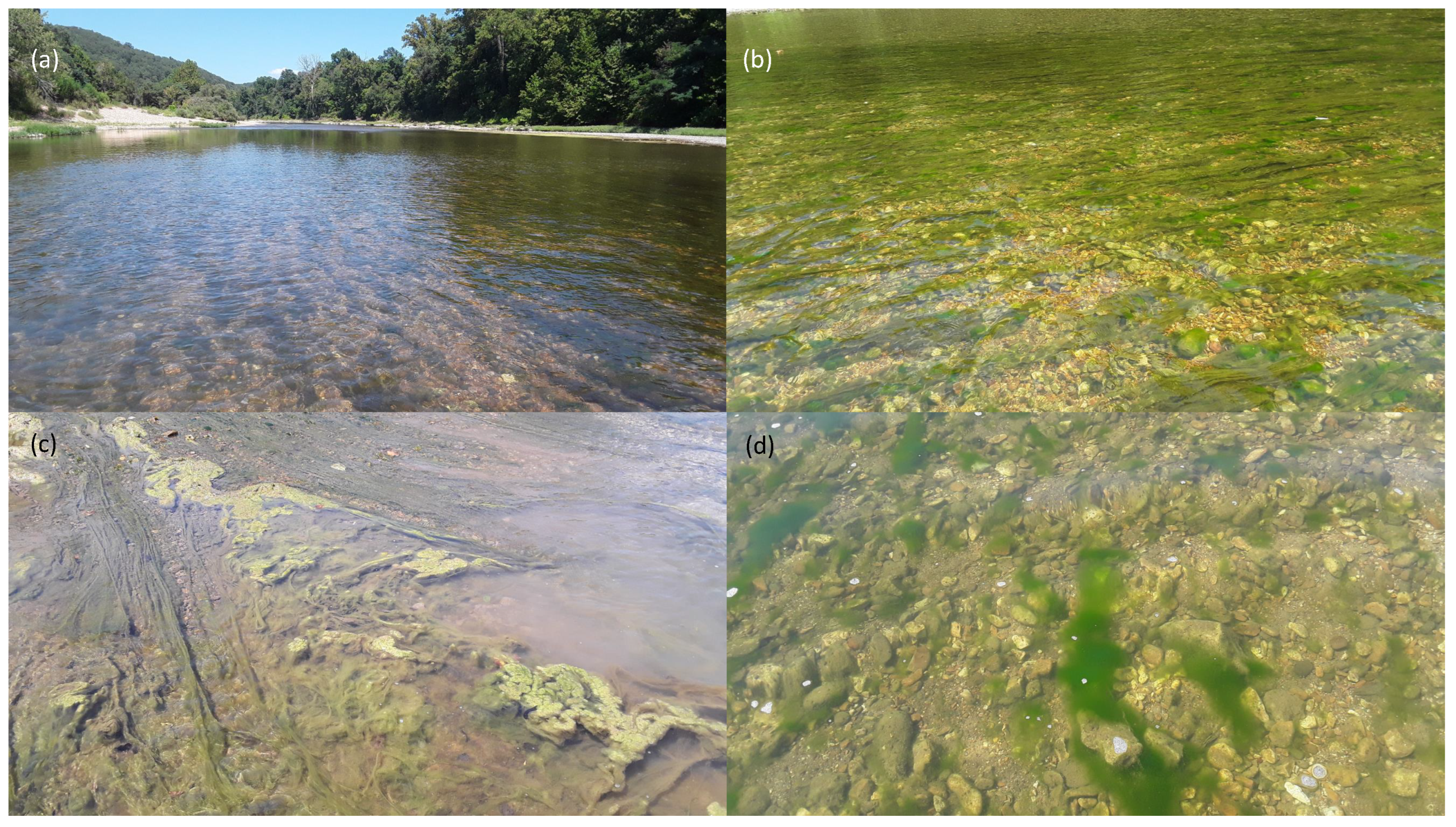
• Field measurements of water depth and algal percent cover from two stream reaches along the Buffalo River captured a range of channel morphologies, with pools up to 1.65 m deep, and algal densities, with complete absence in some places and 100% coverage in others. Benthic algae tended to be more abundant in shallower areas.
• A spectrally based algorithm provided accurate depth estimates, with observed vs. predicted $R^2$ values up to 0.88, when applied to multispectral satellite images and orthophotos acquired from an aircraft. Image-derived depths were biased shallow, however, and only moderately precise, with typical mean biases on the order of 5% of the reach-averaged mean depth and root mean square error values from 30 to 42% of the reach-averaged mean depth.
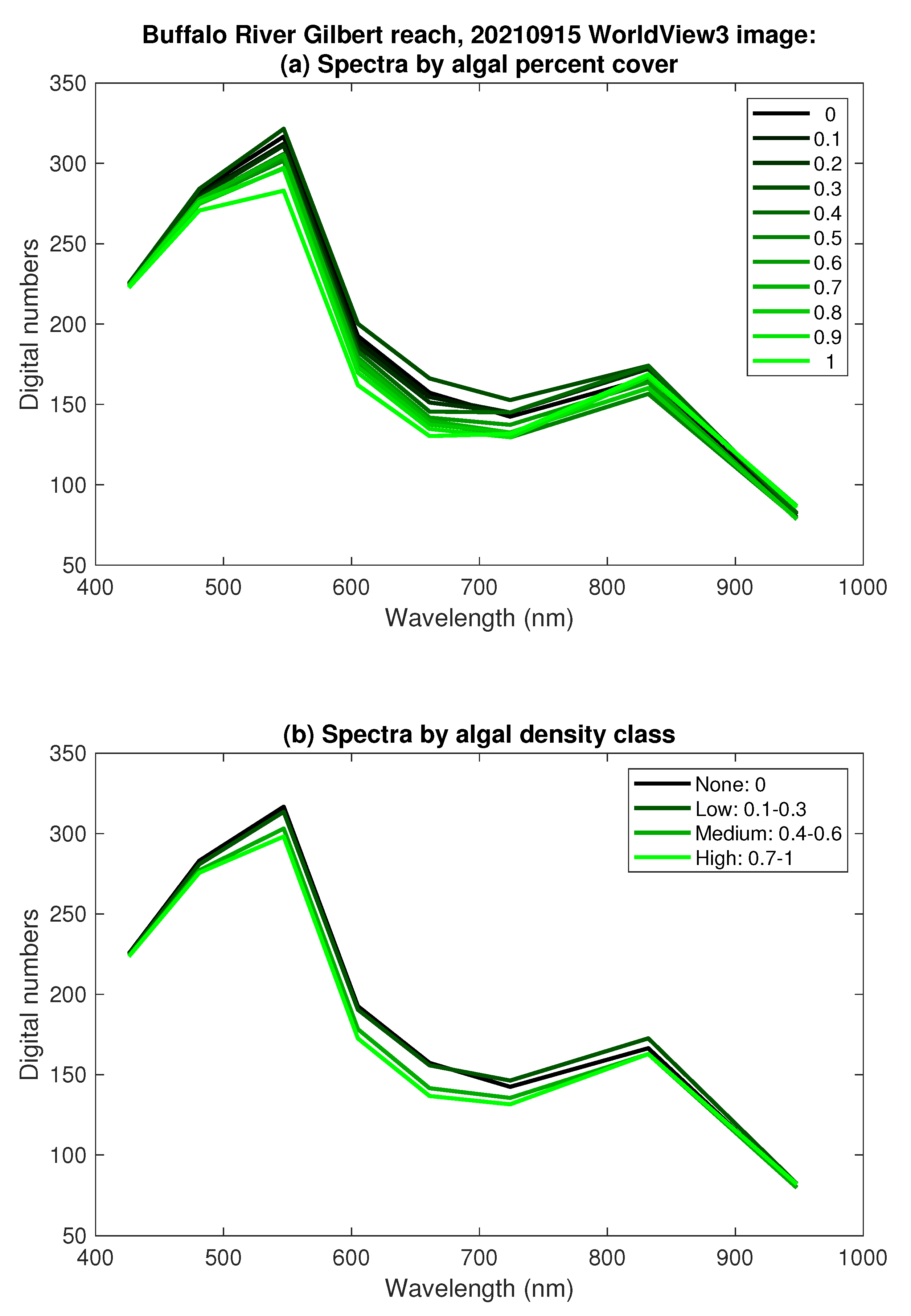
• Spectra extracted from the images at the locations of field measurements were similar across a range of algal percent cover from 0 to 100%, with no clear, consistent distinctions between the 11 discrete levels. Aggregating the data into four algal density classes (none, low, medium, and high) only slightly improved spectral separability, especially for the imaging systems with four bands in the visible and near-infrared.
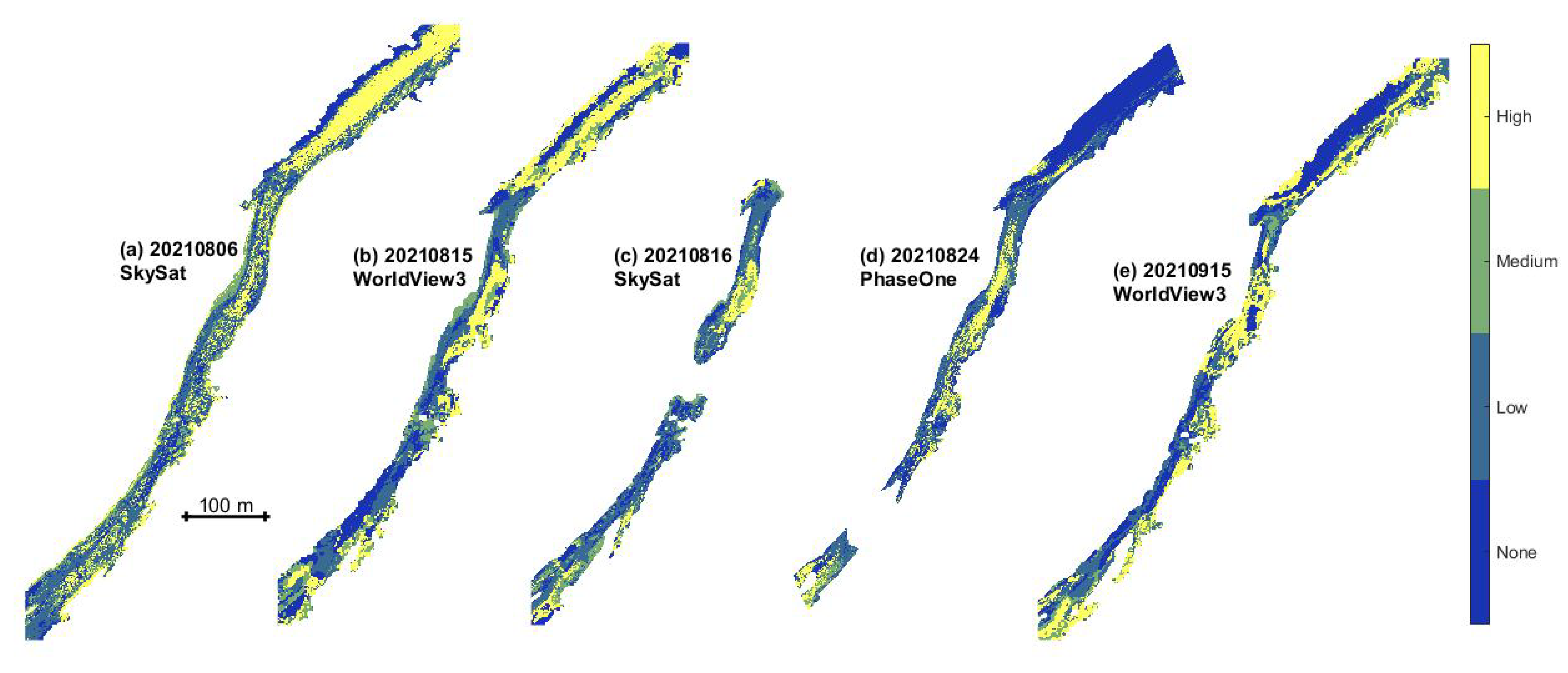
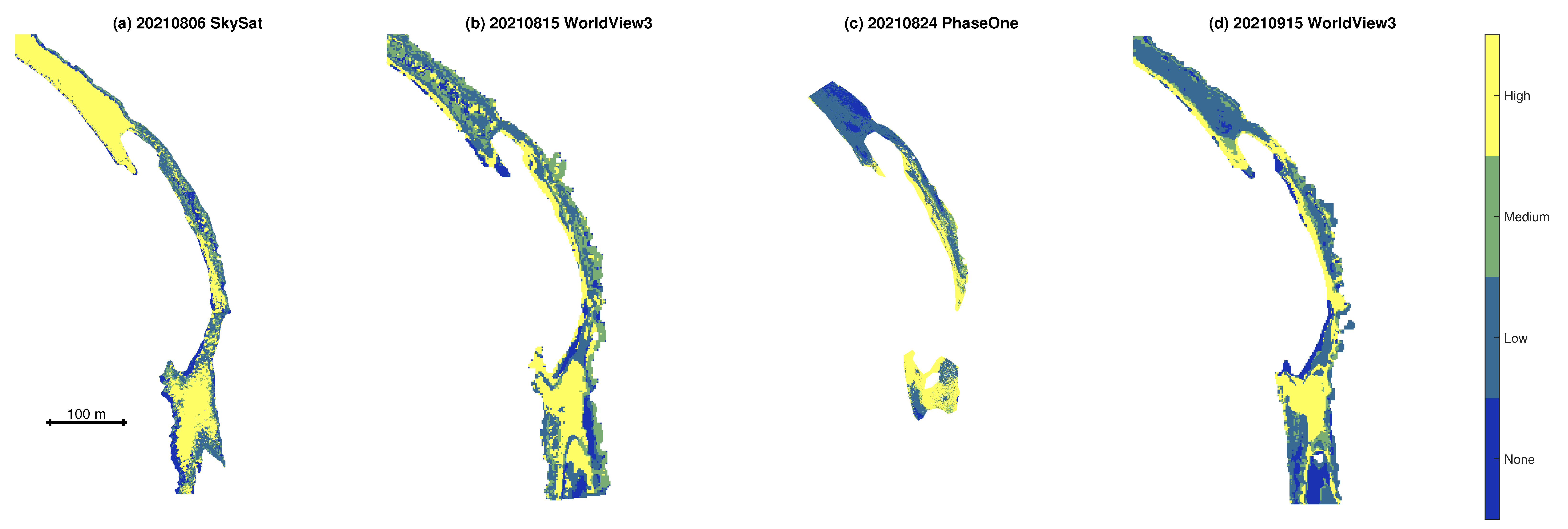
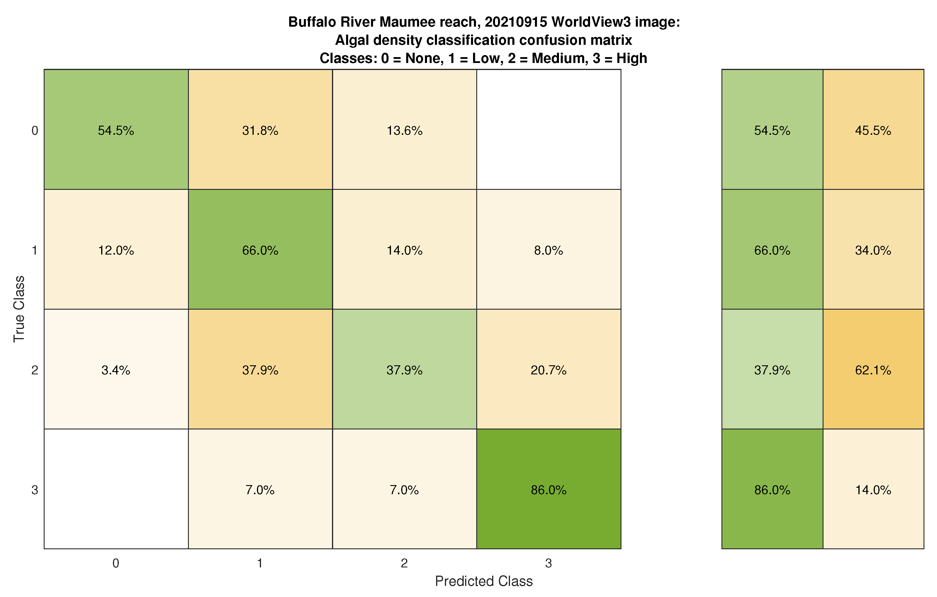
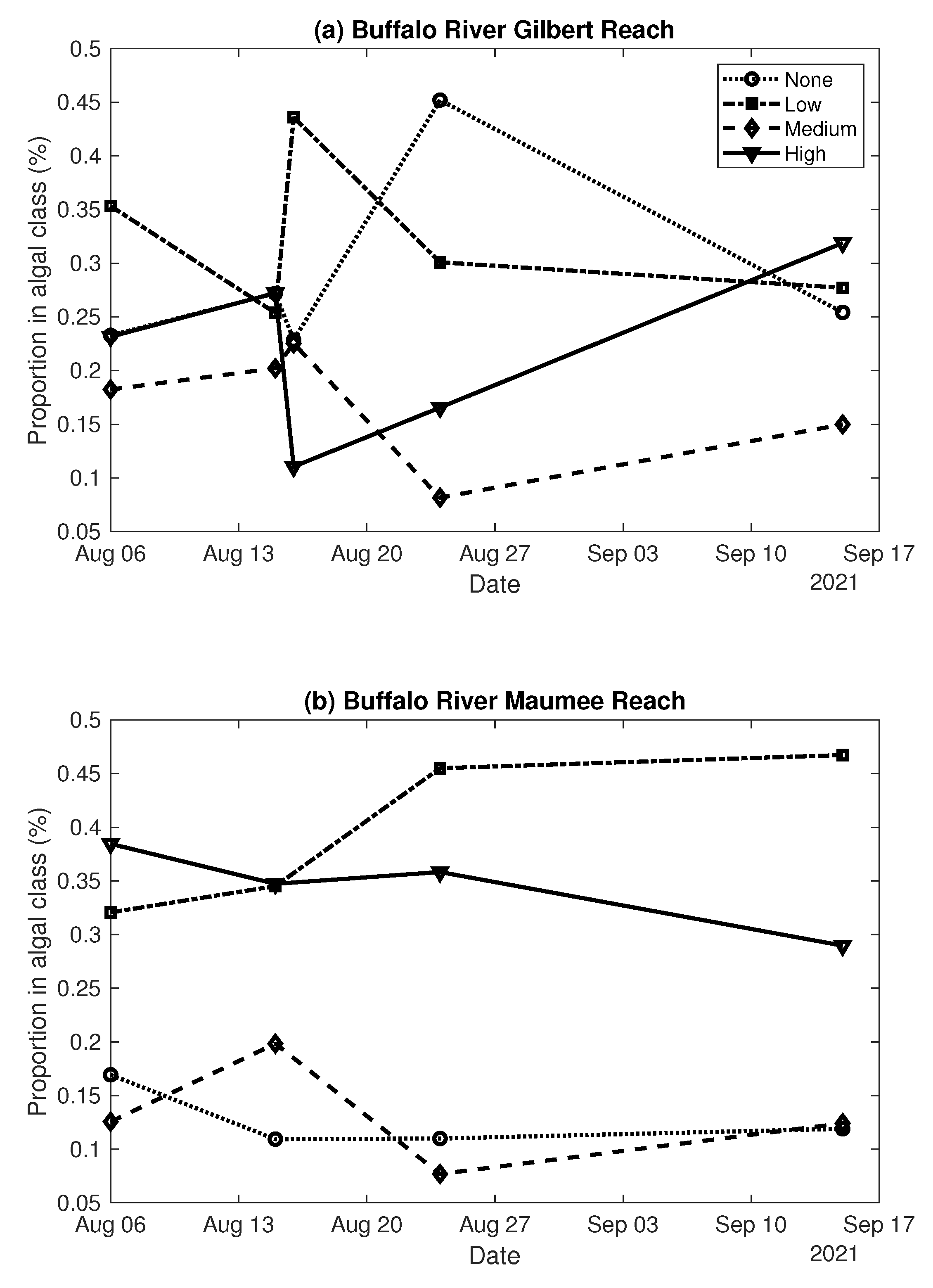
• Classified maps of algal density were produced by augmenting the original spectral bands with depth as an additional predictor variable and then training a bagged trees machine learning algorithm. Although the resulting classifications revealed some consistent spatial patterns and plausible trends over time, overall accuracies were modest, up to 64.6%.
• An important constraint on the reliability of the algal density classifications was the limited spectral resolution of the sensors employed in this study. Hyperspectral techniques capable of exploiting characteristic algal absorption features could enable a shift away from a classification-based framework toward a more quantitative approach focused on estimating algal biomass.

References

1. Ward, J.V.; Tockner, K.; Arscott, D.B.; Claret, C. Riverine landscape diversity. Freshw. Biol. 2002, 47, 517–539. [Google Scholar] [CrossRef] [Green Version]
2. Nilsson, C.; Reidy, C.A.; Dynesius, M.; Revenga, C. Fragmentation and flow regulation of the world’s large river systems. Science 2005, 308, 405–408. [Google Scholar] [CrossRef] [PubMed] [Green Version]
3. Ho, J.C.; Michalak, A.M.; Pahlevan, N. Widespread global increase in intense lake phytoplankton blooms since the 1980s. Nature 2019, 574, 667–670. [Google Scholar] [CrossRef]
4. Kislik, C.; Dronova, I.; Kelly, M. UAVs in Support of Algal Bloom Research: A Review of Current Applications and Future Opportunities. Drones 2018, 2, 35. [Google Scholar] [CrossRef] [Green Version]
5. US Environmental Protection Agency. Learn about Cyanobacteria and Cyanotoxins. Available online: https://www.epa.gov/cyanohabs/learn-about-cyanobacteria-and-cyanotoxins (accessed on 28 December 2021).
6. Cyanotoxin—Zion National Park. Available online: https://www.nps.gov/zion/learn/news/cyanotoxin.htm (accessed on 2 February 2022).
7. Priority Project: Harmful Algal Blooms. Available online: https://doimspp.sharepoint.com/sites/nps-coast/SitePages/Priority-Project--Harmful-Algal-Blooms.aspx#habs-products-proposals (accessed on 1 February 2022).
8. Dodds, W.K.; Bouska, W.W.; Eitzmann, J.L.; Pilger, T.J.; Pitts, K.L.; Riley, A.J.; Schloesser, J.T.; Thornbrugh, D.J. Eutrophication of U.S. freshwaters: Analysis of potential economic damages. Environ. Sci. Technol. 2009, 43, 12–19. [Google Scholar] [CrossRef] [Green Version]
9. Burford, M.A.; Carey, C.C.; Hamilton, D.P.; Huisman, J.; Paerl, H.W.; Wood, S.A.; Wulff, A. Perspective: Advancing the research agenda for improving understanding of cyanobacteria in a future of global change. Harmful Algae 2020, 91, 101601. [Google Scholar] [CrossRef] [PubMed]
10. Brooks, B.W.; Lazorchak, J.M.; Howard, M.D.; Johnson, M.V.V.; Morton, S.L.; Perkins, D.A.; Reavie, E.D.; Scott, G.I.; Smith, S.A.; Steevens, J.A. Are harmful algal blooms becoming the greatest inland water quality threat to public health and aquatic ecosystems? Environ. Toxicol. Chem. 2016, 35, 6–13. [Google Scholar] [CrossRef] [PubMed]
11. Dierssen, H.; Bracher, A.; Brando, V.; Loisel, H.; Ruddick, K. Data needs for hyperspectral detection of algal diversity across the globe. Oceanography 2020, 33, 74–79. [Google Scholar] [CrossRef]
12. Cruz, R.C.; Reis Costa, P.; Vinga, S.; Krippahl, L.; Lopes, M.B. A Review of Recent Machine Learning Advances for Forecasting Harmful Algal Blooms and Shellfish Contamination. J. Mar. Sci. Eng. 2021, 9, 283. [Google Scholar] [CrossRef]
13. Fetscher, A.E.; Howard, M.D.; Stancheva, R.; Kudela, R.M.; Stein, E.D.; Sutula, M.A.; Busse, L.B.; Sheath, R.G. Wadeable streams as widespread sources of benthic cyanotoxins in California, USA. Harmful Algae 2015, 49, 105–116. [Google Scholar] [CrossRef]
14. Graham, J.L.; Dubrovsky, N.M.; Foster, G.M.; King, L.R.; Loftin, K.A.; Rosen, B.H.; Stelzer, E.A. Cyanotoxin occurrence in large rivers of the United States. Inland Waters 2020, 10, 109–117. [Google Scholar] [CrossRef]
15. Wood, S.A.; Kelly, L.T.; Bouma-Gregson, K.; Humbert, J.F.; Laughinghouse, H.D.; Lazorchak, J.; McAllister, T.G.; McQueen, A.; Pokrzywinski, K.; Puddick, J.; et al. Toxic benthic freshwater cyanobacterial proliferations: Challenges and solutions for enhancing knowledge and improving monitoring and mitigation. Freshw. Biol. 2020, 65, 1824–1842. [Google Scholar] [CrossRef] [PubMed]
16. Berkman, J.A.H.; Canova, M.G. Chapter A7. Section 7.4. Algal Biomass Indicators; Technical Report; U.S. Geological Survey: Reston, VA, USA, 2007. [CrossRef]
17. Coffer, M.M.; Schaeffer, B.A.; Salls, W.B.; Urquhart, E.; Loftin, K.A.; Stumpf, R.P.; Werdell, P.J.; Darling, J.A. Satellite remote sensing to assess cyanobacterial bloom frequency across the United States at multiple spatial scales. Ecol. Indic. 2021, 128, 107822. [Google Scholar] [CrossRef]
18. Khan, R.M.; Salehi, B.; Mahdianpari, M.; Mohammadimanesh, F.; Mountrakis, G.; Quackenbush, L.J. A Meta-Analysis on Harmful Algal Bloom (HAB) Detection and Monitoring: A Remote Sensing Perspective. Remote Sens. 2021, 13, 4347. [Google Scholar] [CrossRef]
19. Visser, F.; Wallis, C.; Sinnott, A.M. Optical remote sensing of submerged aquatic vegetation: Opportunities for shallow clearwater streams. Limnologica 2013, 43, 388–398. [Google Scholar] [CrossRef]
20. Visser, F.; Buis, K.; Verschoren, V.; Meire, P. Depth Estimation of Submerged Aquatic Vegetation in Clear Water Streams Using Low-Altitude Optical Remote Sensing. Sensors 2015, 15, 25287. [Google Scholar] [CrossRef] [Green Version]
21. Legleiter, C.J.; Stegman, T.K.; Overstreet, B.T. Spectrally based mapping of riverbed composition. Geomorphology 2016, 264, 61–79. [Google Scholar] [CrossRef] [Green Version]
22. Maritorena, S.; Morel, A.; Gentili, B. Diffuse-reflectance of oceanic shallow waters—Influence of water depth and bottom albedo. Limnol. Oceanogr. 1994, 39, 1689–1703. [Google Scholar] [CrossRef]
23. Dierssen, H.M.; Zimmerman, R.C.; Leathers, R.A.; Downes, T.V.; Davis, C.O. Ocean color remote sensing of seagrass and bathymetry in the Bahamas Banks by high-resolution airborne imagery. Limnol. Oceanogr. 2003, 48, 444–455. [Google Scholar] [CrossRef]
24. Mobley, C.D.; Sundman, L.K.; Davis, C.O.; Bowles, J.H.; Downes, T.V.; Leathers, R.A.; Montes, M.J.; Bissett, W.P.; Kohler, D.D.R.; Reid, R.P.; et al. Interpretation of hyperspectral remote-sensing imagery by spectrum matching and look-up tables. Appl. Opt. 2005, 44, 3576–3592. [Google Scholar] [CrossRef]
25. Slonecker, T.; Kalaly, S.; Young, J.; Furedi, M.A.; Maloney, K.; Hamilton, D.; Richard, E.; Zinecker, E. A Preliminary Assessment of Hyperspectral Remote Sensing Technology for Mapping Submerged Aquatic Vegetation in the Upper Delaware River National Parks (USA). Adv. Remote Sens. 2018, 7, 290–312. [Google Scholar] [CrossRef] [Green Version]
26. Kislik, C.; Genzoli, L.; Lyons, A.; Kelly, M. Application of UAV Imagery to Detect and Quantify Submerged Filamentous Algae and Rooted Macrophytes in a Non-Wadeable River. Remote Sens. 2020, 12, 3332. [Google Scholar] [CrossRef]
27. Legleiter, C.; Hodges, S. Remotely Sensed Data and Field Measurements of Water Depth and Percent Cover of Benthic Algae from Two Reaches of the Buffalo National River in Arkansas Acquired in August and September 2021; U.S. Geological Survey Data Release: Reston, VA, USA, 2022. [CrossRef]
28. Algae and Nurient Sourcing. Available online: https://www.nps.gov/articles/000/algae-and-nutrient-sourcing.htm (accessed on 7 February 2022).
29. Algae Bloom Complaint Form|DEQ. Available online: https://www.adeq.state.ar.us/complaints/forms/algae_complaint.aspx (accessed on 7 February 2022).
30. Fishing—Buffalo National River. Available online: https://www.nps.gov/buff/planyourvisit/fishing.htm (accessed on 7 February 2022).
31. Office of the Federal Register, National Archives and Records Administration. 80 FR 24961—Endangered Species; Marine Mammals; Receipt of Applications for Permit; Office of the Federal Register, National Archives and Records Administration: Washington, DC, USA, 2015.
32. Berkman, D.N.; Lauraas, J. Water Resources Management Plan: Buffalo National River, Arkansas; Technical Report; U.S. National Park Service: Harrison, AR, USA, 2004.
33. U.S. Geological Survey. USGS Water Data for the Nation: U.S. Geological Survey National Water Information System Database. USGS 07056000 Buffalo River near St. Joe, AR. Available online: https://waterdata.usgs.gov/ar/nwis/inventory/?site_no=07056000 (accessed on 22 December 2021). [CrossRef]
34. Leica Zeno GG04 Plus Smart Antenna for High Accuracy Everywhere. Available online: https://leica-geosystems.com/en-us/products/gis-collectors/smart-antennas/leica-zeno-gg04-plus (accessed on 31 January 2022).
35. High-Resolution Imagery with Planet Satellite Tasking. Available online: https://www.planet.com/products/hi-res-monitoring/ (accessed on 7 February 2022).
36. Maxar—Archive Search & Discovery. Available online: https://discover.digitalglobe.com/ (accessed on 7 February 2022).
37. Vanhellemont, Q.; Ruddick, K. Atmospheric correction of metre-scale optical satellite data for inland and coastal water applications. Remote Sens. Environ. 2018, 216, 586–597. [Google Scholar] [CrossRef]
38. Pahlevan, N.; Mangin, A.; Balasubramanian, S.V.; Smith, B.; Alikas, K.; Arai, K.; Barbosa, C.; Bélanger, S.; Binding, C.; Bresciani, M.; et al. ACIX-Aqua: A global assessment of atmospheric correction methods for Landsat-8 and Sentinel-2 over lakes, rivers, and coastal waters. Remote Sens. Environ. 2021, 258, 112366. [Google Scholar] [CrossRef]
39. Lyzenga, D.R. Passive Remote-Sensing Techniques for Mapping Water Depth and Bottom Features. Appl. Opt. 1978, 17, 379–383. [Google Scholar] [CrossRef]
40. Niroumand-Jadidi, M.; Vitti, A.; Lyzenga, D.R. Multiple Optimal Depth Predictors Analysis (MODPA) for river bathymetry: Findings from spectroradiometry, simulations, and satellite imagery. Remote Sens. Environ. 2018, 218, 132–147. [Google Scholar] [CrossRef]
41. Tomsett, C.; Leyland, J. Remote sensing of river corridors: A review of current trends and future directions. River Res. Appl. 2019, 35, 779–803. [Google Scholar] [CrossRef]
42. Legleiter, C.; Roberts, D.A.; Lawrence, R.L. Spectrally based remote sensing of river bathymetry. Earth Surf. Process. Landforms 2009, 34, 1039–1059. [Google Scholar] [CrossRef]
43. Legleiter, C.; Harrison, L.R. Remote Sensing of River Bathymetry: Evaluating a Range of Sensors, Platforms, and Algorithms on the Upper Sacramento River, California, USA. Water Resour. Res. 2019, 55, 2142–2169. [Google Scholar] [CrossRef]
44. Legleiter, C.J. The optical river bathymetry toolkit. River Res. Appl. 2021, 37, 555–568. [Google Scholar] [CrossRef]
45. Breiman, L. Random forests. Mach. Learn. 2001, 45, 5–32. [Google Scholar] [CrossRef] [Green Version]
46. Stackelberg, P.E.; Belitz, K.; Brown, C.J.; Erickson, M.L.; Elliott, S.M.; Kauffman, L.J.; Ransom, K.M.; Reddy, J.E. Machine Learning Predictions of pH in the Glacial Aquifer System, Northern USA. Groundwater 2021, 59, 352–368. [Google Scholar] [CrossRef] [PubMed]
47. Congalton, R.G.; Green, K. Assessing the Acuracy of Remotely Sensed Data: Principles and Practices; CRC Press: Boca Raton, FL, USA, 1999; p. 137. [Google Scholar]
48. Glibert, P.M. Eutrophication, harmful algae and biodiversity—Challenging paradigms in a world of complex nutrient changes. Mar. Pollut. Bull. 2017, 124, 591–606. [Google Scholar] [CrossRef] [PubMed]
49. Overstreet, B.T.; Legleiter, C. Removing sun glint from optical remote sensing images of shallow rivers. Earth Surf. Process. Landforms 2017, 42, 318–333. [Google Scholar] [CrossRef]
50. Legleiter, C.; Mobley, C.D.; Overstreet, B.T. A framework for modeling connections between hydraulics, water surface roughness, and surface reflectance in open channel flows. J. Geophys. Res. Earth Surf. 2017, 122, 1715–1741. [Google Scholar] [CrossRef]
51. Aleksandra, K.; Fantina, M.; Marco, S.; Ferrarin, C.; Giacomo, M.G. Assessment of submerged aquatic vegetation abundance using multibeam sonar in very shallow and dynamic environment. The Lagoon of Venice (Italy) case study. In Proceedings of the 2015 IEEE/OES Acoustics in Underwater Geosciences Symposium (RIO Acoustics), Rio de Janeiro, Brazil, 29–31 July 2015; pp. 1–7. [Google Scholar] [CrossRef]
52. Held, P.; von Deimling, J.S. New feature classes for acoustic habitat mapping—A multibeam echosounder point cloud analysis for mapping submerged aquatic vegetation (SAV). Geosciences 2019, 9, 235. [Google Scholar] [CrossRef] [Green Version]
53. Legleiter, C.; Fosness, R. Defining the Limits of Spectrally Based Bathymetric Mapping on a Large River. Remote Sens. 2019, 11, 665. [Google Scholar] [CrossRef] [Green Version]
54. Rousso, B.Z.; Bertone, E.; Stewart, R.; Hamilton, D.P. A systematic literature review of forecasting and predictive models for cyanobacteria blooms in freshwater lakes. Water Res. 2020, 182, 115959. [Google Scholar] [CrossRef]
55. Iiames, J.S.; Salls, W.B.; Mehaffey, M.H.; Nash, M.S.; Christensen, J.R.; Schaeffer, B.A. Modeling Anthropogenic and Environmental Influences on Freshwater Harmful Algal Bloom Development Detected by MERIS Over the Central United States. Water Resour. Res. 2021, 57, e2020WR028946. [Google Scholar] [CrossRef]
56. Paine, E.C.; Slonecker, E.T.; Simon, N.S.; Rosen, B.H.; Resmini, R.G.; Allen, D.W. Optical characterization of two cyanobacteria genera, Aphanizomenon and Microcystis, with hyperspectral microscopy. J. Appl. Remote Sens. 2018, 12, 036013. [Google Scholar] [CrossRef]
57. Slonecker, T.; Bufford, B.; Graham, J.; Carpenter, K.; Opstal, D.; Simon, N.; Hall, N. Hyperspectral Reflectance Characteristics of Cyanobacteria. Adv. Remote Sens. 2021, 10, 66–77. [Google Scholar] [CrossRef]
58. Slonecker, T.; Simon, N.; Graham, J.; Allen, D.; Bufford, B.; Evans, M.; Carpenter, K.; Griffin, D.; Hall, N.; Jones, D.; et al. Hyperspectral Characterization of Common Cyanobacteria Associated with Harmful Algal Blooms (Ver. 2.0, October 2020); U.S. Geological Survey Data Release: Reston, VA, USA, 2020. [CrossRef]
Figure 1. Photos of benthic algae along the Gilbert reach of the Buffalo River. (a) Provides an overview looking upstream and (bd) illustrate the diversity of algal forms present within the reach. Photographs used with permission from Derek Filipek of the US National Park Service.
Remotesensing 14 00953 g001
Figure 2. Study area along the Buffalo National River in northern Arkansas, USA. False-color infrared images (near-infrared band displayed as red, red band displayed as green, and green band displayed as blue) from each type of sensor evaluated in this study are shown in (ac) for the Maumee reach and in (fh) for the Gilbert reach. An inset map indicating the location of the Buffalo River within the south-central United States is provided in (d) and an overview of the study area is shown in (e). The overall flow direction is from west to east, which is from the bottom to the top of the images in (ac) and from left to right in the images in (eh).
Remotesensing 14 00953 g002
Figure 3. Hydrograph for the USGS streamgage (#07056000) on the Buffalo River near St. Joe, Arkansas, showing variations in discharge during the study. The dates of image acquisition and field data collection are indicated by the labeled vertical lines.
Remotesensing 14 00953 g003
Figure 4. Diagrammatic representation of the workflow for remote sensing of benthic algae in rivers.
Remotesensing 14 00953 g004
Figure 5. Field observations from the Gilbert reach of the Buffalo River. Measurements of water depth are summarized in a (a) map and (b) histogram. Similarly, the data on percent cover of benthic algae are presented in (c,d). The background image is an orthophoto produced from the airborne data collected the same day as the field measurements. Flow direction is from the bottom toward the top of the image.
Remotesensing 14 00953 g005
Figure 6. Field observations from the Maumee reach of the Buffalo River. Measurements of water depth are summarized in a (a) map and (b) histogram. Similarly, the data on percent cover of benthic algae are presented in (c,d). The background image is an orthophoto produced from the airborne data collected one day before the field measurements. Flow direction is from the bottom toward the top of the image.
Remotesensing 14 00953 g006
Figure 7. Optimal band ratio analysis (OBRA) of the September 15 WorldView3 image of the Maumee reach. (a) Matrix representing the strength of the X vs. d relation for each possible combination of numerator λ 1 and denominator λ 2 bands in terms of the regression R 2 . (b) Calibrated relationship between X and d for the optimal band ratio. (c) Depth map produced by applying this relation to the spatially filtered water-only image.
Remotesensing 14 00953 g007
Figure 8. Accuracy assessment of depth estimates derived from the 15 September 2021, WorldView3 image of the Maumee reach. (a) Distribution of depth retrieval errors, defined as the field-measured depth minus the image-derived depth. (b) Map illustrating the spatial pattern of depth retrieval errors. (c) Observed (field-measured) vs. predicted (image-derived) depths regression.
Remotesensing 14 00953 g008
Figure 9. Example spectra extracted from the 15 September 2021, WorldView3 image of the Gilbert reach and then grouped by (a) percent cover of benthic algae and (b) algal density class. The spectra plotted here are the means of all pixels with each level of percent cover and density class.
Remotesensing 14 00953 g009
Figure 10. Time series of algal density classification maps produced from various images of the Gilbert reach of the Buffalo River. (a) SkySat image from 6 August 2021; (b) WorldView3 image from 15 August 2021; (c) SkySat image from 16 August 2021; (d) PhaseOne image from 24 August 2021; (e) WorldView3 image from 15 September 2021.
Remotesensing 14 00953 g010
Figure 11. Time series of algal density classification maps produced from various images of the Maumee reach of the Buffalo River. (a) SkySat image from 6 August 2021; (b) WorldView3 image from 15 August 2021; (c) PhaseOne image from 24 August 2021; (d) WorldView3 image from 15 September 2021.
Remotesensing 14 00953 g011
Figure 12. Example confusion matrix for a classification of algal density produced from the 15 September WorldView3 image of the Maumee reach of the Buffalo River. The color scale represents the proportion of pixels in each combination of true class and predicted class, with green tones indicating higher proportions and lighter orange indicating a lower proportion. The smaller array on the right side of the figure lists the producer’s accuracy in the right column and the omission error in the left column.
Remotesensing 14 00953 g012
Figure 13. Variations over time in the proportion of image pixels assigned to each algal density class for the (a) Gilbert and (b) Maumee reaches.
Remotesensing 14 00953 g013